Investigation of the maximum amplitude increase from the Benjamin–Feir instability

This is an initial work on ’Extreme Waves in Hydrodynamics Laboratory’. Extreme waves here refer to very high amplitude, steep, waves that can appear suddenly from a relatively calm sea. Although extreme waves are very rare and unpredictable, they are still very dangerous to ships in case they meet.

We model the problem of extreme waves using dispersive wave modes. The specific property of dispersion is that waves with different wave length propagate with different phase velocities. In the following we assume that the wave field has a frequency spectrum that is localized around one frequency. Then the envelope of the wave field is described by the NLS equation [3]. The NLS equation is an amplitude equation for describing the change of envelope of a wave group. This equation is very instrumental in understanding various nonlinear wave phenomena : it arises in studies of unidirectional propagation of wave packets in a energy conserving dispersive medium at the lowest order of nonlinearity [4].

In this paper we analyze the behavior of the wave group envelope using both linear and nonlinear theories. Linear theory predicts exponential growth of the amplitude when certain conditions are satisfied—the Benjamin–Feir instability [4]. However, when the amplitude becomes large nonlinear effects must be taken into account, that, as it turns out, will prevent further exponential growth. The aim of this paper is to find the maximum amplitude of waves when the amplitude growth is triggered by the Benjamin–Feir instability. Also, we investigate how this maximum amplitude depends on the growth rate parameter from the Benjamin–Feir instability.

To investigate the instability of the NLS plane–wave solution, we perturb the $\xi$–independent function $A(\tau)$ with a small perturbation of the form $\epsilon(\xi,\tau)=A(\tau)\,B(\xi,\tau)$. We look for the cases where under a small perturbation the amplitude of the plane wave solution grows in time [3]:

Substituting (10) into (6), and ignoring nonlinear terms we obtain the linearized NLS equation :

We seek the solutions of (11) in the form

where $B_{1},B_{2}\in\mathbb{C}$, $k_{0}+\kappa$ is local wavenumber, $\kappa$ is modulation wavenumber, and $\sigma\in\mathbb{C}$ is called the growth rate. If Re ($\sigma)>0$, then the perturbed solution of the NLS equation grows exponentially. This is the criterion for the so–called Benjamin–Feir instability of a one–wave mode with modulation wavenumber $\kappa$ [3].

Substituting the function $B(\xi,\tau)$ in (12) into (11) yields a pair of coupled equations that can be written in matrix form as follows

Nontrivial solution to (13) can exist only if the determinant of the left hand side matrix is zero. This condition reads as follows

We have the following cases :

• •

  The growth rate $\sigma$ is real and positive if $\kappa^{2}<2\frac{\gamma}{\beta}\,r_{0}^{2}$. This corresponds to Benjamin–Feir instability. For specified values of $\kappa$, the perturbation amplitude is exponentially amplified in time [3].

• •

  The growth rate $\sigma$ is purely imaginary if $\kappa^{2}>2\frac{\gamma}{\beta}\,r_{0}^{2}$. This corresponds to a plane–wave solution that has bounded amplitude for all time [3].

Thus, the range of instability is given by

It is easy to find that the ’strongest’ instability occurs at $\kappa_{\textmd{\scriptsize{max}}}=\sqrt{\frac{\gamma}{\beta}}\,r_{0},$ where the maximum growth rate is $\sigma_{\textmd{\scriptsize{max}}}=\gamma\,r_{0}^{2}$. Figure 1 shows the plot of growth rate $\sigma$ as a function of modulation wavenumber $\kappa$ for $r_{0}=\beta=\gamma=1$.

We can write the solution of the linearized NLS equation as

with $\sigma(\kappa)=\kappa\,\sqrt{2\,\beta\,\gamma\,r_{0}^{2}-\beta^{2}\,\kappa^{2}}$. Since this solution is obtained from the linearized NLS equation, it is only valid if amplitudes are small. When the time is increased, the amplitude increases exponentially and the linearized theory becomes invalid. Therefore, we cannot use the solution from the linearized equation to investigate the behavior of the maximum amplitude increase due to the Benjamin–Feir instability. Fortunately, there exists an exact solution to the NLS equation that describes the exact behavior of the wave profile and that corresponds to the Benjamin–Feir instability.

In this section we investigate the relation between the maximum amplitude of a certain solution of the NLS equation and the modulation wavenumber $\kappa$ in the instability interval. For simplicity, we choose the amplitude $r_{0}=1$, and the coefficients $\beta=\gamma=1$. An exact solution, the so–called soliton on finite background, in short SFB, (sometimes also called the second most important solution), of the NLS equation is given by [1] :

where $0<\kappa<\sqrt{2}$ and $\sigma(\kappa)=\kappa\sqrt{2-\kappa^{2}}$.
For $\kappa=1,$ we have

Figure 2 shows the plot of $\left|\psi\right|$ from (18) as a function of $\xi$ and $\tau$. Note that $\psi(\xi,\tau)$ is a $2\pi$–periodic function with respect to $\xi$ variable.

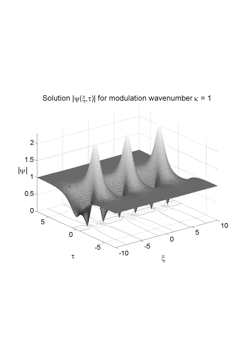
In the following, we analyze the solution (17) in detail. The behavior for this SFB as $\tau\rightarrow\pm\infty$ is given by

Because of this property the solution (17) is called as SFB. For a ’normal’ soliton, the elevation vanishes at infinity : the ’normal’ soliton is exponentially confined. For SFB, the solution is a similar elevation on top of the finite (nonzero) background level, here the normalized value 1.

Write the solution in the form $\psi(\xi,\tau)=u(\xi,\tau)\,e^{\,i\,\tau}$, where $u(\xi,\tau)$ where $u$ describes the amplitude and the exponential part expresses oscillations in time. Let us investigate the behavior of $u(\xi,\tau)$ in time. For that consider the limiting behavior of $\partial_{\tau}u$ as $\tau\rightarrow\pm\infty$. We have

If $\xi\neq\frac{\pi}{2\,\kappa}$, then

and

If $\xi=\frac{\pi}{2\,\kappa}$, then

and

Next, let us find the relation between the maximum amplitude of the exact solution (17) with modulation wavenumber $\kappa$, where $0<\kappa<\sqrt{2}$. The maximum value of the complex amplitude is at $\xi\equiv 0\;(\textmd{mod}\;2\pi)$ and when $\tau=0$. So, we have

Using the approximation $\sqrt{1+a}\approx 1+\frac{1}{2}a$ for small $a$, and apply it to our formula ($a=-\frac{1}{2}\kappa^{2}$), we obtain

As a result, the maximum factor of the amplitude amplification is

Figure 3 shows the plot of the maximum amplitude $|\psi|_{\textmd{\scriptsize{max}}}$ as a function of modulation wavenumber $\kappa$.

To summarize, Figure 4 compares the plot of the dispersion relation $\Omega$ and its quadratic approximation (leads to the NLS equation), the growth rate $\sigma$ (which is related to Benjamin–Feir instability), and the maximum amplitude of $\psi$ as functions of wavenumber $k$.

In this paper we modelled surface waves in wave tanks of hydrodynamics laboratories using the NLS equation. We analyzed the linearized NLS equation and obtained that its solutions have tendency to grow exponentially. We considered also the exact solution known as SFB of the NLS equation, that is the continuation of this linear instability. Using this, we found the maximum amplitude in space and time when the modulation wavenumber is in the interval of the Benjamin–Feir instability. The main result of this paper is that the maximum factor of the amplitude amplification due to the Benjamin–Feir instability is three. As we can see from Figure 4, the growth rate from the Benjamin–Feir instability does not determine the maximum amplitude amplification of the SFB. The results of this paper will be used in the further study of relating the Benjamin–Feir instability and the Phase–Amplitude equations.

Acknowledgement

This work is executed at University of Twente, The Netherlands as part of the project ’Extreme Waves’ TWI.5374 of the Netherlands Organization of Scientific Research NWO, subdivision Applied Sciences STW.

References

- [1] N. N. Akhmediev and A. Ankiewicz. Solitons—Nonlinear Pulses and Beams, volume 5 of Optical and Quantum Electronic Series. Chapman & Hall, first edition, 1997.
- [2] E. Cahyono. Analytical Wave Codes for Predicting Surface Waves in a Laboratory Basin. PhD thesis, University of Twente, Faculty of Mathematical Sciences, June 2002.
- [3] L. Debnath. Nonlinear Water Waves. Academic Press, Inc., 1994.
- [4] A. Scott. Nonlinear Science—Emergence and Dynamics of Coherent Structures. Oxford University Press, 1999.
- [5] C. Sulem and P. L. Sulem. The Nonlinear Schrödinger Equation—Self Focusing and Wave Colapse, volume 139 of Applied Mathematical Sciences. Springer–Verlag New York Inc., 1999.
- [6] E. van Groesen. Wave groups in uni–directional surface–wave model. Journal of Engineering Mathematics, 34(1-2):215–226, 1998.