Roaming moduli space using dynamical triangulations
J. Ambjørn, J. Barkley, and T.G. Budd
a The Niels Bohr Institute, Copenhagen University
Blegdamsvej 17, DK-2100 Copenhagen Ø, Denmark.
email: ambjorn@nbi.dk, barkley@nbi.dk
b Institute for Theoretical Physics, Utrecht University,
Leuvenlaan 4, NL-3584 CE Utrecht, The Netherlands.
email: t.g.budd@uu.nl
Abstract
In critical as well as in non-critical string theory the partition function reduces to an integral over moduli space after integration over matter fields. For non-critical string theory this moduli integrand is known for genus one surfaces. The formalism of dynamical triangulations provides us with a regularization of non-critical string theory. We show how to assign in a simple and geometrical way a moduli parameter to each triangulation. After integrating over possible matter fields we can thus construct the moduli integrand. We show numerically for and non-critical strings that the moduli integrand converges to the known continuum expression when the number of triangles goes to infinity.
PACS: 04.60.Ds, 04.60.Kz, 04.06.Nc, 04.62.+v.
Keywords: quantum gravity, lower dimensional models, lattice models.
1 Introduction
Non-critical string theory, or two-dimensional Euclidean quantum gravity coupled to matter, has been a fruitful laboratory for studying aspects of string theory as well as quantum gravity. Solving these theories one has had the advantage to have both a lattice version of the theory and a continuum field theory formulation. The lattice version has been denoted the dynamical triangulation model () or the matrix model of non-critical string theory. It can be solved, basically by combinatorial methods, exemplified by the use of matrix models. The explicit solution of the continuum model uses the fact that the Liouville theory is a (special) conformal theory. For observables which can be calculated by both approaches agreement is found.
Since non-critical string theory is described by conformal field theory we know that conformal invariance is implemented. However, the precise manifestation of this invariance, and how it is related to the moduli space of the underlying surfaces (i.e. to the part of the surface geometry left invariant under conformal transformations) has been rather limited. That dynamical triangulations or matrix models contain precise information about the moduli space is on the other hand obvious. For instance it was shown in [1] that the resolvent of the matrix model has an expansion in terms of so-called moments, where the coefficients in the double scaling for the genus terms are precisely the intersection indices of moduli space for genus Riemann surfaces with any number of punctures. It was also shown how these matrix models in the double scaling limit can be related to the Kontsevich matrix model which provides a representation of the generating function for these intersection indices [1, 2]. Much work has later expanded on these results [3], but we are in these approaches far from the naive and simple idea which was the starting point for and matrix models, namely that provides a regularization of the path integral of non-critical strings and thus the moduli parameters should appear in the same simple way as they formally appear in the string path integral.
One problem when using matrix models is that most observables which can be calculated analytically are of global nature: integrated correlation functions of matter fields or the partition function as a function of various boundary states. Further, the comparison with continuum results is only possible for the simplest topologies of the surfaces: spherical topology, disc topology and (only recently [4]) cylindrical topology. It is simply difficult to perform calculations in the framework of Liouville theory for higher genus surfaces. However, there is a narrow window where one can test in more detail if the matrix models, or the framework of dynamical triangulations, actually agree with the continuum expressions for higher genus surfaces in the naive way mentioned above. We know the partition function for genus one surfaces of non-critical strings expressed as an integral over the moduli parameter of the torus [5]. Integrating out the matter fields, using the conformal anomaly, worldsheet conformal invariance ensures that the remaining integrand of the partition function is only an (explicitly known) function of the moduli parameters. We can now in principle compare this integrand to the integrand which we obtain using dynamical triangulations as a regularization of the non-critical string theory. Which integrand do we obtain using dynamical triangulations? For each triangulation we have a continuous, piecewise linear geometry. To each such geometry we can associate moduli parameters (as described below). Each geometry will appear with a certain weight which depends on the matter we have coupled to the surface. If we have triangles we will in this way obtain a number of points in moduli space and when goes to infinity we expect these discrete points converge to a density distribution which should be proportional to the integrand of non-critical string theory. The possibility of performing such a comparison was pioneered by Kawai and collaborators[6]. They found good qualitative agreement between the non-critical string integrand and the density constructed from dynamical triangulations. The purpose of this article is to improve this test, making it quantitative, and also present a more general setup than the one used in [6]. We also show how one can measure the moduli parameters for higher genus triangulations, but unfortunately there is presently no theoretical calculation with which we could compare such results which would be easy to generate numerically.
2 The setup
In string theory we can integrate out the conformal matter fields on the worldsheet by the conformal anomaly. This is true also for non-critical string theory. The partition function of e.g. a bosonic string in dimensions can be written as
| (1) |
where the integration over worldsheet geometries of genus is implemented by integrating over metrics , gauge fixed to conformal gauge , denoting a fiducial background metric depending on (for ) complex moduli parameters parametrizing the complex structure of the genus Riemann surface and being a modular invariant measure. The denote the Faddeev-Popov ghosts associated with the partial gauge fixing to conformal gauge, denotes the Liouville field and finally is the Liouville action:
| (2) |
The constants in the Liouville action are chosen such that the conformal invariance is maintained in the quantum theory in accordance with the bootstrap approach of David, Distler and Kawai [7], i.e.
| (3) |
For a fixed value of the moduli parameters one can in principle perform the integration over the bosonic fields and the ghost fields. One obtains contributions from zero modes and appropriate determinants. However, only in the case of genus one is the integration over the zero mode trivial, the reason being that . In this case one obtains just the standard result from critical string theory [5]. Thus, if we consider the situation where we fix the world sheet area to be , i.e. trade the cosmological constant in (2) for the area , we obtain
| (4) |
In (4) denotes the central charge of the conformal matter theory coupled to 2d gravity, the complex moduli parameter of the complex structure we are integrating over and is the region in the complex plane to which belongs. Finally is given by:
| (5) |
We want to test how well the non-critical string theory regularized by approximates this formula. We will further restrict ourselves to the cases and . We do so in order to obtain the best statistics in the numerical tests we perform. The case is chosen to avoid to have to update matter fields in addition to the geometry, when we use Markov chain Monte Carlo simulations to generate configurations. The case is chosen in order to have a non-trivial matter system coupled to gravity which can be easily handled numerically. For there exists a recursive algorithm which allows us to avoid constructing Markov chains and generate directly random triangulations with the correct weight, including the matter fields [8].
The set-up is thus the following: Using we can fix the area, like in (4). This is done by fixing the number of triangles, since all triangles are viewed as identical in the formalism. A triangulation can thus in principle be viewed as representing a piecewise linear geometry. As we will show below there is a natural way to associate with such a piecewise linear geometry a moduli parameter. For the ensemble of piecewise linear geometries constructed from identical equilateral triangles, each triangulation with the topology of a torus, we will then have an approximation to the continuum distribution . We will investigate if and how the corresponding distribution of the moduli parameter constructed from the ensemble characterized by triangles converges to the continuum distribution for . A priori it is not clear that there should be a convergence at all. Given a continuum area , we usually think of the lattice area as , being the link length of the triangulation. Thus keeping fixed and taking dictates how one should think of the lattice link length . However, the corresponding piecewise linear surface will in general not be anything like a smooth surface. In fact we know now that it with probability one will be fractal with a Hausdorff dimension different from two [9]. The situation is thus quite similar to the one encountered for the ordinary path integral of a particle: with probability one a path in the path integral is nowhere differentiable and has a Hausdorff dimension different from one. As long as we think of the ensemble of piecewise linear surfaces in this way one would not be too worried about the highly fractal structure of the geometry associated with a generic triangulation in the ensemble for , and we know that for global observables one obtains identical results using continuum Liouville theory and the ensemble, taking . However, it is less clear if an assignment of a moduli parameter as we are going to do it, by analogy between differential forms and “discrete differential forms” on simplicial complexes, even if very natural, will work for the “wild” generic triangulations we meet in the ensemble. Recall for instance that the spectral properties of the Laplacian defined even on the simplest piecewise linear surfaces are different from the generic spectral properties of the Laplacian defined on a smooth geometry, because one should, when analyzing the spectrum, view the piecewise linear geometry as a geometry with conical singularities at the vertices [11]. Since we are actually using properties of the Laplacian to determine the moduli parameter, one could be worried whether the assignment using discrete differential forms makes sense in the present context. However, we will find that the assignment works beautifully!
Let us start by showing how to determine the moduli parameter if given a two-dimensional Riemannian geometry of a genus one surface. Let denote the exterior derivative and its adjoint (the co-differential) with respect to the standard inner product defined on -forms, for two-dimensional surfaces:
| (6) |
where is the Hodge dual11 1 In components the Hodge dual of a -form on a -dimensional Riemannian manifold is defined as: form of . In particular we have for two 1-forms:
| (7) |
where and , in some coordinate system . The Hodge Laplacian
| (8) |
maps -forms to -forms, and for 1-forms on a genus surface the kernel is -dimensional, constituting the so-called harmonic differentials. For a genus one surface the vector space of harmonic 1-forms is thus two-dimensional. We can find it by solving
| (9) |
which express that a harmonic 1-form has a vanishing curl and divergence.
Let us choose two closed curves and on the torus that generate the fundamental group. It is then possible to choose “dual” harmonic 1-forms and , i.e. harmonic forms which satisfy:
| (10) |
For the torus the moduli parameter can be defined in the following way: by the uniformization theorem any metric on a surface is conformally related to a constant-curvature metric. For the torus it is a zero-curvature metric, and starting from the Euclidean plane we obtain such a flat torus by identifying opposite sides in a parallelogram. Let the two sides of the parallelogram be vectors and , represented as complex numbers. The moduli parameter is defined as . It is clearly invariant under translations, rotations and global scaling of the parallelogram and we can assume that . However, there are finite diffeomorphisms of the torus which cannot be obtained continuously from the identity, and which we will insist do not change the partition function. These transformations do not leave invariant but will change it according to
| (11) |
The transformations (11) constitute a transformation group called the modular group and it is isomorphic to . In the integral (4) we are instructed only to integrate over points which cannot be identified by the action of the modular group via (11), i.e. is a so-called fundamental domain of in the upper half-plane: no pair of points within it can be connected by a modular transformation and any point outside it can be reached from a unique point inside by some modular transformation. A standard choice of fundamental domain is:
| (12) |
We will use this fundamental domain in the rest of the article. Of course it is not unique: for example any modular transformation will transform it to another fundamental domain.
Given a metric and the curves , is determined by the formula
| (13) |
To prove this formula we note that we can choose periodic coordinates and , both with period 1, such that and run around in the and direction, respectively and such that metric takes the form:
| (14) |
where is a local scale factor and represents a flat metric with determinant 1. The parallelogram can now be represented in the Euclidean plane as shown in Fig. 4 and the is thus explicitly given by
| (15) |
the factor enforcing . Since harmonicity of the 1-forms is preserved under conformal transformations, we clearly have that and and the inner product can be read off from the definition (7):
| (16) |
The determined by formula (13) lies in the upper half-plane, but not necessarily in the fundamental domain defined in (12). We use (11) to find the modular transformation which maps it to .

The formula (13) can be applied directly to the piecewise linear geometries encountered in the formalism since the notion of -forms and an exterior derivative acting on these forms can be defined in a natural way. For a detailed definition for piecewise linear geometries, defined by triangulations where the lengths of the links between vertices and are given, we refer to standard textbooks [12]. In the case of the formulas become very simple because all link lengths are identical, and similarly all areas of triangles are identical. Thus for the piecewise linear surfaces the definitions become identical to the “abstract” definition of discrete differentials used on simplicial complexes to study the discrete versions of cohomology as a more general setup than the De Rham cohomology of ordinary differential forms. A discrete -form is in the simplicial complex context defined by assigning a real number to each oriented -simplex . Changing orientation of the simplex changes the sign of the assigned real number. The linear space of -forms has dimension equal to the number of -simplices in the triangulation. For the scalar product corresponding to (6) we simply choose
| (17) |
The exterior derivative is defined as
| (18) |
where the sum is over all -subsimplices in and the sign factor signifies the orientation of the subsimplex relative to the orientation of . Again , the co-differential, is defined as the adjoint of with respect to the scalar product (17). To be explicit, consider the 1-forms. The 1-forms take values on the oriented links. Denote the vertices in the triangulation and the links when vertices and vertices are connected by a link oriented from to . Similarly triangles are denoted . Thus we have and
| (19) |
where the summation is over all links incident on vertex . If one wants to relate 1-forms defined this way to continuum notation, one can heuristically think of the 1-form as
| (20) |
Using (20) and appealing to Stokes theorem will be proportional to the curl associated with triangle , and similarly Gauss’ theorem makes proportional to the divergence assigned to the cell dual to vertex . We note that using the definition (19) it is easy to show [12] that for a triangulation of genus the equations and have solutions, in agreement with the continuum result referred to above.
Finally we define a path in the triangulation as a path of links. Thus we have a natural integration of 1-forms along a path:
| (21) |
We now have all the ingredients for the construction of the moduli parameter for a piecewise linear triangulation belonging to the ensemble of genus 1. First identify two non-contractible loops and which generate the fundamental group. Next solve and to find the two-dimensional space of harmonic 1-forms. Finally select from this space the two 1-forms and which satisfy the discrete analogy of (10), i.e.
| (22) |
Let us finally note that we can use the harmonic 1-forms and to obtain an explicit embedding of a triangulation into a parallelogram in the Euclidean plane. In the continuum, choosing coordinates such that the generating curves and run around in the and directions, respectively, we have . Thus, knowing we can recover the coordinates by integration. We now apply this to our triangulation using the two harmonic 1-forms we have constructed for the triangulation. For each link we view the vector as representing the link in the Euclidean plane precisely in the heuristic sense of eq. (20). Starting from an arbitrary vertex we can now reconstruct the triangulation in the Euclidean plane. Fig. 1 shows an example of such a reconstruction. Recall that a function is harmonic if and only if it has the mean value property: the value of a harmonic function at the center of a circle is equal to the integral of the function along the circle divided by the length of the circle. The discrete map from the triangulation to the Euclidean plane is harmonic in the sense that any vertex is located at the center of mass of its neighbors.
Fig. 2 shows other embeddings of triangulations of the torus in the Euclidean plane. These triangulations are much larger than the one shown in Fig. 1, each consisting of triangles. The triangulation to the left is from the ensemble of triangulations considered in the next section (2d gravity without matter fields), while the triangulation to the right is picked from the ensemble of triangulations describing conformal matter coupled to 2d gravity (to be described in detail in Sec. 4). Shown in red are also the shortest non-contractible loops, which we will discuss later. In addition Fig. 2 captures qualitatively the fractal structure of the ensemble of triangulations, to be analyzed below.


The method described above for calculating the moduli of a genus one surface (and the moduli of a genus one triangulation) has a relatively simple generalization to higher genus surfaces and triangulations. This is outlined in appendix A. Below we describe the result of computer simulations which extract the moduli of genus one triangulations. It is unproblematic to do the same for genus triangulations, , although the moduli space now has the (real) dimension , but we have no continuum expressions with which we can compare the sampled distributions of moduli parameters, as already mentioned.
3 Measuring for
In order to measure for we perform Monte Carlo simulations starting out with a triangulation of the torus, constructed from triangles. For a description of how to perform such simulations we refer to [14]. The Monte Carlo simulations consists of “moves” which change the triangulation locally, preserving and the topology. After sufficiently many local moves we will have created a statistically independent triangulation. The number of moves needed on average for this increases with . From the independent configurations constructed this way we now calculate by
- (1)
identifying two non-contractible link-loops and which generate the fundamental group of the torus,
- (2)
constructing the harmonic differentials by solving the divergence and curl equations, and ,
- (3)
forming linear combinations such that (22) is satisfied,
- (4)
constructing using (13),
- (5)
In this way we construct a distribution of ’s which we can compare with the theoretical distribution. The most computer intensive part of the calculation is step (2), the identification of the two-dimensional subspace of (discrete) harmonic 1-forms. Fig. 3 shows a plot of the -distribution.

The fundamental domain is non-compact. If we place the flat torus as shown in Fig. 4 we clearly have a torus very elongated in the vertical direction for large imaginary values of .

Of course this does not necessarily reflect a property of the original triangulation since we are using a (discrete) conformal map to embed the triangulation in the Euclidean plane. However, on average one would expect a large imaginary value of to reflect a -torus with short non-contractible loops in one “direction” compared to the possible lengths of non-contractible loops in the other “direction”. For the triangulations there are two restrictions entering: by definition there is a shortest allowed loop length since we count the loop length in an integer number of links. Also, for a finite , there is a limit to how long one can make geodesic loops. Thus we expect for a finite that our -distribution of ’s will fail for large imaginary values of , but it should improve if (I) we increase and (II) we use -ensembles which allow smaller non-contractible loops. The second point can easily be tested in the following way: let us start with a -ensemble of “regular” triangulations . By that we mean triangulations where each vertex has at least order three and where two vertices are connected by at most one link. The dual graphs are graphs without tadpole and self-energy subgraphs. On this ensemble a shortest non-contractible loop is of length 3. We could instead allow two vertices to be connected by two different links, belonging to different triangles. We call this ensemble . The dual graphs are graphs without tadpoles, but with self-energy subgraphs (except the simplest ones which would result in vertices of order two). The shortest non-contractible loop length for this ensemble is clearly 2. Finally we consider the ensemble where we allow a link to loop to its own vertex. In terms of dual graphs we now allow tadpole graphs (but exclude still the simplest self-energy graphs to maintain that all vertices in the triangulation have an order larger than or equal three22 2 We should stress that there is nothing important related to requirement that the vertex order is larger than or equal 3. We just maintained it because our original computer program had it built in.). We denote this ensemble . The shortest loop length is one for this -ensemble. In Fig. 5 we have shown the probability distribution of for a fixed and compared it to the theoretical, continuum distribution. The distribution is significantly closer to the continuum distribution for large as expected. We also checked explicitly that the improvement was due to non-contractible loops of length 1 by calculating the distribution of for the sub-ensemble of which had no non-contractible loops of length 1. The results then agreed with the results for the ensemble. In the rest of this article we will thus only use the ensemble , which we for simplicity just call the -ensemble.

Let us now turn to point (I) above, the dependence. Fig. 6 shows that the distribution agrees very well with the theoretical distribution for the large value of used, and Fig. 7 shows the deviation from the theoretical distribution for different ’s.


Thus there seems to be a nice convergence to the correct distribution for . However, let us try to understand in more detail the relation between the geometry of the triangulations and the moduli parameter . Due to (discrete) conformal invariance the relation cannot be very direct. We observed above that the minimal length of a non-contractible loop was important for the distribution (for fixed ). Let us classify a triangulation according to the length of its shortest non-contractible loop. In the piecewise linear geometry of such a loop will be a geodesic curve in the sense. Thus we expect that its length scales anomalously with respect to the area [9, 10]. We can check this explicitly by determining shortest closed loops for random triangulations in the -ensemble using the method described in appendix B (see also [13]). The result for the expectation value is shown in Fig. 8 and indeed we find that
| (23) |
where is the Hausdorff dimension of the -ensemble. One can view the triangulation to the left in Fig. 2 as an illustration of relation (23), the length of the shortest non-contractible loop shown in red is of the order , not of the order . Further implications of eq. (23) have been discussed in a recent paper [13].

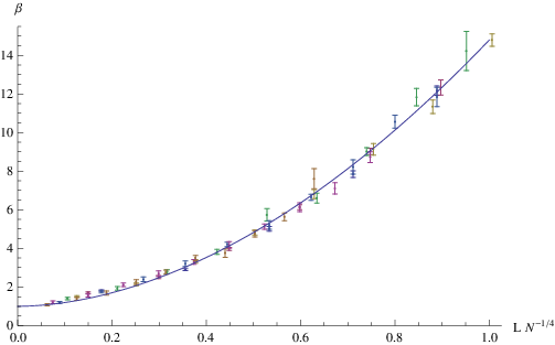
From the continuum formulas (4) and (5) we expect the distribution to fall off like for much larger than 1. This is indeed in agreement with Fig. 6. However, if we split the -ensemble in subsets according to , we observe a universal dependence in terms of the “dimensionless” variable :
| (24) |
The constants 13.7 and 1.85 are the result of a best fit to the data (see Fig. 9) and are not that precisely determined. The important point (apart from the universality) is that the main contribution for large comes from small . Thus statistically there is a clear relation between small ’s in the triangulation and large ’s in the embedded Euclidean plane. And “small” can be quantified as follows: since a typical linear extension of the triangulation, measured in geodesic distances, will be , and “small” means small compared to this linear extension.
Finally, let us emphasize that the existence of a small in a triangulation does not imply that is large. For instance both independent holonomy directions could have small non-contractible loops. As an extreme there could even be non-contractible loops of length one in both directions. In this case the embedding maps (like the ones shown in Fig. 1 and Fig. 2) to the Euclidean plane could be extreme, having only a few large triangles and the rest of the triangulation concentrated on a very little area. In such a case would not be large, rather we would just have a nice illustration of the power of local conformal transformations. When is not too large we indeed observe such situations since the smallest values of are not that rare.
4 Measuring for
We want to test eq. (4) for . As mentioned is chosen because it is easier to address numerically than other matter systems coupled to two-dimensional Euclidean quantum gravity. The matter coupled to quantum gravity has several realizations. A minimal -conformal field theory, , co-prime integers larger than 1, has central charge and, coupled to quantum gravity, the string susceptibility for surfaces with spherical topology is . Formally a model will have and . It does not really belong to the minimal models and there is no Kac table associated with . Nevertheless one can find a fermionic conformal field theory which formally can be identified with a (1,2) model [15]. It can (partly) be viewed as a topological field theory. This is the reason the matter coupled to quantum gravity is often called topological 2d gravity. However, there exists another formal representation of the matter system coupled to 2d Euclidean quantum gravity. It also leads to after integrating over the matter fields, and in fact the value was first calculated using this representation in the formalism [16].
Consider the partition function (1) for the bosonic string in dimensions. Since the correspond to Gaussian fields we can perform the integration over these fields and we will obtain
| (25) |
Here denotes the Laplace-Beltrami operator on the background geometry and the prime signifies that the zero mode has been removed when calculating the determinant of . If we consider as a formal parameter, is special since we just get the determinant itself, as one would have for a suitable fermionic system, and since is the central charge for positive integer, we formally have a system where . The -formalism tells us that we should represent the regularized partition function (1) as
| (26) |
where the summation is over all triangulations of genus in a suitable -ensemble. denotes the bare cosmological constant of the 2d quantum gravity theory (the Liouville cosmological constant in the continuum notation), the number of triangles in and is symmetry factor of the triangulation , i.e. the order of the automorphism group of the graph . Finally denotes the (discretely defined) Laplacian on the -surface, which we take to be the usual graph Laplacian of the graph dual to the triangulation. We can trade the cosmological constant for the area of the (triangulated) surface. Since each triangle has the same area in the formalism, this implies keeping the number of triangles fixed and our partition function becomes
| (27) |
where denotes the -ensemble with triangles. We expect to approach the continuum for via the identification , where denotes the length of the links in the triangulation.
It is well-known that the determinant of a graph Laplacian (with the zero-mode removed) is equal to the number of spanning trees on the graph.33 3 For a given connected graph, a spanning tree is a connected subgraph which contains all the vertices, but which contains no loops, i.e. closed paths of links. Therefore where denotes the number spanning trees of the graph dual to the triangulation . It was this representation of the combinatorial Laplacian which allowed to authors of [16] to solve the model for and prove that , a result which was controversial at the time it was published.
The partition function becomes
| (28) |
where denotes the set of genus triangulations which are “decorated” by spanning trees. Thus two such triangulations are counted as different even if they as triangulations are identical, but if they have different “embedded” spanning trees.
In [8] it was realized that this formula, in the case of genus zero (), could be used in computer simulations to generate directly, by a recursive algorithm, a set of graphs which have the correct weight, including the matter fields. Thus, in order to test the properties of matter coupled to 2d quantum gravity, one can directly generate a set of independent graphs of arbitrary size and circumvent the problem of generating statistically independent configurations by local Monte Carlo updating, a problem which becomes increasingly time consuming when is large. This way of dealing numerically with the system has been used extensively to study the fractal properties of quantum gravity [17]. However, both the original solution of the model and the successive applications used in a crucial way that . For our application we need a generalization of the method to higher genera, or at least to genus one. Such a method is described for the simplest case in the next section using a very recent result from [19]. In appendix A we sketch the procedure for larger genus.
4.1 Random generation of decorated torus triangulations
We will now describe an algorithm which generates a random triangulation of genus with triangles decorated with a spanning tree. The algorithm is designed such that any decorated triangulation is sampled with equal probability. The class of triangulations we are considering is the most general one, i.e. we allow for triangles to be glued to themselves and two different triangles are allowed to be glued along more than one edge as long as the triangulation remains connected and the resulting piecewise linear manifold remains homeomorphic to a surface of genus .
Given a triangulation together with a spanning tree on its dual graph, we consider the set of edges of the triangulation which are not intersected by the spanning tree. This set of edges forms a graph consisting of links and containing loops. If we cut open the triangulation along these links, we obtain a triangulation of the disc with a boundary consisting of links. This triangulated disc is completely characterized by the structure of a trivalent tree with internal vertices (see the top part of Fig. 10). To get back to the original triangulation, the boundary edges of the disc have to be glued pairwise. This suggests that any decorated triangulation can be obtained by combining a tree and a pairwise gluing.
Let us make this a bit more precise. We can view the vertices of the spanning tree as located at the center of the triangles. The order of the vertices (the number of links to which they belong) can be one, two or three. By construction they are located at triangles where two, one or no links have been cut open. Let us add two, one or no “external” links to the vertices. One can visualize this as the external lines still being located in the triangle to which the spanning tree vertex belongs, and “pointing” to the triangle links which have been cut open. In this way the spanning tree has been extended to a tree where the vertices have become internal vertices of order three and where external links have been added. We mark one of the external links in order to have a rooted tree. In this way the tree becomes precisely of the form of a binary tree. The external links are now, by construction, in 1-to-1 correspondence with the boundary links of the disc. The pairwise gluing of the edges of the disc to a genus surface corresponds to a pairwise identification of the external lines in the binary tree such that the resulting trivalent graph can be placed on a genus surface without any lines crossing (this is the meaning of the trivalent graph being of genus ). Such a pairwise gluing of a polygon is known as a unicellular map [19] (or one-face map) of genus with “half-edges”.

The above arguments show that we can generate a random decorated triangulation by separately generating a random trivalent planar tree and a random unicellular map. We then use the unicellular map to connect the external lines of the trivalent tree.
As already remarked the random trivalent planar trees with a marked external line are in 1-to-1 correspondence with binary trees. There exists efficient algorithms to generate such trees, see e.g. [18] section 7.2.1.6.
The major problem is to implement the random unicellar map. The model was originally solved for because it was understood that a genus zero unicellular map with half-edges is given simply by a planar tree with one half-edge marked [16]. Fig. 10 illustrates this: the identification of the half-edges has to form “rainbow” diagrams in order that one creates a genus zero surface. The corresponding planar trees are again related to binary trees and can thus be easily generated randomly.
To generate a torus we need a random genus one unicellular map with half-edges. Luckily in [19] an explicit connection was found between unicellular maps of genus and genus . In particular, for a genus zero unicellular map a procedure is given in which three distinct vertices are identified and the half-edges are relabeled in such a way that one obtains a genus one unicellular map. It is shown that any genus one unicellular map can be obtained through such a procedure in exactly two different ways (see [19], proposition 1 and corollary 1).
Let us briefly summarize the procedure (see Fig. 10 for an example). We label the half-edges of the -gon anti-clockwise by and we provide them with the corresponding orientation, such that they have a starting vertex and a final vertex. A unicellular map of genus zero is fixed by giving a list of pairs of integers which tell us which edges to glue. After the gluing we have a tree with vertices (see Fig. 10) of which we randomly select three distinct ones. For each of them we select from the set of half-edges having that vertex as its final vertex the smallest index. We denote these indices by , , and and reorder them such that . The resulting unicellular map of genus one is now given by gluing according to in which we replace , where
| (29) |
We refer the [19] for the actual proof of this statement.
4.2 Numerical results for
We use the above described algorithm to generate an ensemble of graphs and we use this to perform the same measurements as for . Let us record the distribution. It is shown in Fig. 11.


We have a perfect fit even for a relatively small triangulation of 8000 triangles. In fact we have seen no deviation from the theoretical curve not compatible with the error-bars, so we have not addressed the approach to the theoretical curve as a function of as we did for .
We measured the expectation value of the length of the shortest non-contractible loop and the result is shown in Fig. 12.

As for we expect anomalous scaling according to (23), only now is no longer equal to 4, but given by the formula [20]
| (30) |
for . The data shown in Fig. 12 is in perfect agreement with (30), which for becomes . Eq. (30) was earlier verified with good precision for genus zero surfaces by directly measuring the area enclosed within a circle of geodesic radius and showing that , with given by (30) [17]. As already noticed, (23) can be viewed as an independent verification of the anomalous scaling of geodesic distance. Another rather stunning confirmation that the intrinsic structure of 2d quantum gravity is governed by the dimensionless quantity , being the area of the 2d universe, a geodesic distance, can be obtained by looking closer at the actual probability distribution of the length of the shortest non-contractible loop as a function of . In Fig. 13 we have shown the distribution for a range of stretching from 126 to more than . In Fig. 14 we show that all of these are well described by
| (31) |
This finite size scaling over such an amazing range of ’s explains why we could hardly see any deviation from the continuum theoretical result in Fig. 11: already is in some sense very close to the limit according to (31).


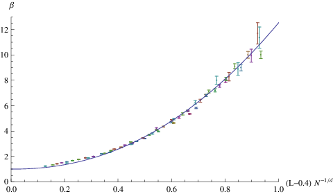
For a conformal field theory with central charge we expect from the continuum formulas (4) and (5) that the distribution will fall off like for much larger than 1. We already checked this for and from Fig. 11 it is clear that it is also true for . Again, if we split the -ensemble in subsets according to , we observe a universal dependence in terms of the “dimensionless” variable (Fig. 15):
| (32) |
The constants and are different from the ones, and we have included a ‘‘shift’’44 4 The “shift” can be viewed as a simple way to compensate for discretization effects for small ’s. We expects a formula like (24) or (32) to reflect a continuum dependence where is the continuum length and is the continuum area . While can be arbitrarily small, this is of course not the case for which is an integer. A priori there will be discretization effects if is not much larger than 1. However, it is know that a shift can reduce the discretization effects [10, 21] and for it does improve the fit. For the shift is not important and we left it out in (24). in the integer values by , but the message is the same: at the boundary of moduli space the distribution is completely determined by the smallest ’s, where the independent statement of “small” is that is small.
5 Discussion
Starting from a path integral approach to two-dimensional Euclidean quantum gravity coupled to matter fields, we need a regularization of the path integral if we want to have a definition of the theory which is not only formal. The formalism of dynamical triangulation is such a regularization. One can view the -formalism in two ways. In the first a triangulation represents a continuum piecewise linear geometry. Thus the geometry is considered flat except at the vertices. At the vertices geometric quantities such as curvature, which involve derivatives of the geometry, can be singular. In a natural way the curvature has a delta-function distribution, being located at the vertices. One can take the point of view that the vertex represents a conical singularity with a certain deficit angle, but it might not be important to take such a literal continuum interpretation. At least it is a cumbersome road to take since we are interested in a limit where the number of vertices goes to infinity, and since we consider the triangles as building blocks, keeping them all as equilateral triangles, the deficit angles are not going to zero even if we consider triangulations with an increasing number of building blocks and even if we rescale all side lengths of the triangles to zero. Alternatively we might simply consider a triangulation as a lattice realization of a 2d geometry, where not too much emphasis should be put on the piecewise linear structure.
The analogy with the textbook derivation of the ordinary path integral in quantum mechanics might be useful: the path integral is obtained by discretizing the time interval, which leads to a multidimensional integral . We can now choose to view the points as vertices in a piecewise linear path connecting the initial point and the final point . With such a choice, the piecewise linear paths with vertices becomes a subset of the full set of continuous paths connecting and , which enter into the continuum path integral. It can be shown that this subset of piecewise linear paths is a dense set in the limit when the right norm is used to define distances between continuum paths, namely the norm compatible with the Wiener measure (see [14] for a detailed discussion). However, we are not forced to take such a point of view for the particle path integral. We could simply view as a lattice version of the formal continuum expression and whatever action we use in the continuum, we choose a suitable discretized lattice version of derivatives etc. Then, when the lattice spacing goes to zero we expect to obtain the continuum theory. Universality in the Wilsonian sense is then the key ingredient for obtaining a universal continuum limit. For the free relativistic particle this was analyzed in detail in [14] and the universality can be shown to be a consequence of the central limit theorem.
Presently we have no rigorous mathematical definition of the formal measure over geometries but it is natural to believe that it involves the integration over all continuous geometries55 5 Clearly, using the standard, formal, continuum procedure summarized in (1), one ends up with an integration over the field . The path integral over clearly involves fields which are continuous but nowhere differentiable. The same will then be true for the corresponding geometries defined by the metric , where is a fixed background metric.. If we take the first point of view advocated for the path integral of the particle, we can choose to consider the -ensemble as a subset of the continuous geometries which, when the number of triangles goes to infinity while the length of the links goes to zero in such a way that the is kept fixed, hopefully becomes dense in the set of continuous geometries with volume . However, contrary to the situation for the particle path integral, we cannot prove this since we do not presently know the norm which defines distances in the space of continuous two-dimensional geometries. As mentioned in the Introduction there is indeed some evidence that the -set of piecewise linear geometries can be viewed as dense in the set of continuous geometries, since a number of global quantities calculated using the formal continuum path integral agree with the corresponding quantities calculated using the -ensemble.
However, the actual use of the -ensemble, both in analytical calculations and numerical simulations, is more in the spirit of the second point of view advocated for the path integral of the particle. According to this point of view we consider the -formalism as some conveniently chosen UV lattice representation of the two-dimensional geometries, where one should not put too much emphasis on the detailed piecewise linear geometric interpretation. Indeed, in the actual numerical simulations one measures geodesic distance using lattice links or dual links, not the actual geodesic distance in the piecewise linear geometry. Also, one is using discrete differences as substitutes for derivatives, rather than trying to formulate the field theory on a geometry with conical singularities. Similarly, one often considers discrete spin systems, like the Ising model, representing some conformal field theories. Such systems are of course only defined on a lattice. All numerical evidence as well as analytical calculations support the Wilsonian idea that lattice details are relatively unimportant when taking the continuum limit.
It is with this second point of view in mind that we have analyzed the moduli structure provided to us by the -ensemble. We have not tried to view the triangulation as piecewise linear geometry with conical singularities to which one can associate a precise conformal structure as for instance described in [22]. Rather, we have just imitated a standard analytic construction of the moduli parameter by replacing the harmonic differentials with suitable discrete differentials. This is in the spirit of the lattice approach. The conclusion: it works almost perfectly. In particular the results, where we were not depending on Markov chain Monte Carlo simulations, are in perfect agreement with the continuum results. Our numerical experiments also provide us with additional evidence that the anomalously scaling geodesic distance plays a key role in any deeper understanding of observables in quantum gravity theories.
Acknowledgments
JA would like to thank the Institute of Theoretical Physics and the Department of Physics and Astronomy at Utrecht University for hospitality and financial support. He also acknowledge financial support by the Danish Research Council (FNU) from the grant “quantum gravity and the role of black holes”. TB acknowledge support by the Netherlands Organisation for Scientific Research (NWO) under their VICI program.
Appendix A Generalization to higher genus
The way we have set up the moduli measurements in section 2 allows for a rather straightforward generalization to surfaces of genus larger than 1.66 6 A method similar to the one described here has been previously employed in a completely different context in [23]. For such surfaces the complex structure is characterized by the Teichmüller space of complex dimension . Identifying explicitly complex moduli parameters is a hard task and one which we will not pursue for general genus. Instead we will use a direct generalization of the genus 1 moduli parameter in the complex upper half-plane to matrices in the -dimensional Siegel upper half-plane , known as period matrices [24]. The Siegel complex upper half-plane consists of all symmetric complex by matrices that have a positive-definite imaginary part. A period matrix corresponding to a surface is known to completely determine its complex structure. For genus we can actually identify with Teichmüller space, but for Teichmüller space appears as a non-trivial submanifold sitting in (as is apparent from comparing their dimensions).
In order to define the period matrix for a Riemannian manifold we have to first choose a set of closed curves which generate the fundamental group and which satisfy
| (33) |
where denotes the oriented intersection number. The space of harmonic 1-forms is -dimensional and it is possible to choose a basis dual to the curves and in the sense that
| (34) |
A complex basis of holomorphic 1-forms is given by
| (35) |
where is the Hodge dual. The period matrix is then given by in terms of the matrices
| (36) |
We can express these integrals in terms of the inner-products , and by using the Riemann bilinear relations [24], which state that any two closed 1-forms and satisfy
| (37) |
Therefore
| (38) |
and
| (39) |
Another consequence of (37) is that
| (40) | |||||
These formulae we can directly apply to piecewise linear geometries by replacing and by their discrete counterparts and the inner-product by the discrete one from (17). For genus we used (40) to establish the normalization of the discrete inner product leading to the expression for in (13). For genus there is an overall ambiguity in the definition of because (40) is not exactly satisfied (up to overall factor) due to discretization artefacts. However, we expect (and we have confirmed this numerically for genus 2) that for large random surfaces (40) is close to a multiple of the identity matrix with high probability. In that case we can unambiguously normalize the inner-product and determine .
The modular group which acts on the upper half-plane as in (11) generalizes to the action of the symplectic group on the Siegel upper half-plane . Fundamental domains can again be worked out but become increasingly cumbersome for larger genus (see e.g. [25]).
Finally let us mention that our algorithm for generating random surfaces coupled to conformal matter can be straightforwardly extended to genus . The only missing ingredient is a construction of a random unicellular map of genus . Here again we can use results from [19] in which for any genus an explicit bijection is found between the set of unicellular maps of genus and a union of sets of unicellular maps of lower genus with a particular number of distinguished vertices.
Appendix B Finding shortest non-contractible loops
First let us present a method of constructing curves in the triangulation that generate the fundamental group. Inspired by the methods described in Sec. 4.1 we generate an arbitrary spanning tree on the graph dual to the triangulation. Then we consider the set of edges of the triangulation that are not intersected by this spanning tree.77 7 Notice that in the case of randomly generated triangulations coupled to conformal matter we have these ingredients already by construction. As mentioned in Sec. 4.1 the graph formed by these edges contains cycles, where is the genus of the triangulation. To extract these cycles we choose an arbitrary vertex in and generate a spanning tree for based at . This tree will contain all but of the edges of . Adding any of the remaining edges to the tree will lead to a cycle and therefore to a unique closed path based at . By rearranging (and if necessary composing) the paths thus obtained we arrive at a canonical set of generators , i.e. a set that satisfies (33), for the fundamental group of the triangulation.
Once we have such a set of generators we can establish for any closed curve whether it is contractible or not by computing its oriented intersection number with the generators . The curve is contractible if and only if all these intersection numbers vanish. To make this test more efficient notice that we can easily construct by hand for each generator a closed discrete 1-form , i.e. satisfying , such that the intersection number of a curve with is equal to the discrete integral of along that curve. Hence, a closed curve is non-contractible if the integral of at least one of the 1-forms is non-vanishing.
Given a vertex we can find a shortest non-contractible loop based at by performing a so-called breadth-first search in the edge-graph of the triangulation starting at . Once we encounter a vertex that we have already visited before, we have implicitly established a loop in the edge-graph. The first such loop we meet that is non-contractible will automatically have minimal length.
Now in principle we can repeat this procedure for each vertex in the triangulation to find the overall shortest non-contractible loop (or rather a non-contractible loop of minimal length as there usually more than one). However in general the set of vertices for which we have to perform this procedure can be greatly reduced. Indeed, we known that any non-contractible loop will intersect at least one of the generators , so it suffices to take to consist of all vertices contained in the . In order to obtain such a set with as few vertices as possible it is worthwhile to first spend some time to shorten the . This will result in a set with a number of vertices of the order with the number of triangles. Since a single breadth-first search involves a number of steps of the order , the full algorithm will have an expected run-time of the order , which amounts to for and for .
References
- [1] J. Ambjorn, L. Chekhov, C. F. Kristjansen, Y. Makeenko, Nucl. Phys. B404 (1993) 127-172. [hep-th/9302014].
- [2] J. Ambjorn, C. F. Kristjansen, Mod. Phys. Lett. A8 (1993) 2875-2890. [hep-th/9307063].
- [3]
L. Chekhov, B. Eynard, N. Orantin,
JHEP 0612 (2006) 053.
[math-ph/0603003].
L. Chekhov, B. Eynard, JHEP 0603 (2006) 014. [hep-th/0504116]. - [4]
E. J. Martinec,
[hep-th/0305148].
N. Seiberg, D. Shih, JHEP 0402 (2004) 021. [hep-th/0312170].
J. Ambjorn, S. Arianos, J. A. Gesser, S. Kawamoto, Phys. Lett. B599 (2004) 306-312. [hep-th/0406108].
J. Ambjorn, J. A. Gesser, Phys. Lett. B659 (2008) 718-722. [arXiv:0707.3431 [hep-th]]. Phys. Lett. B653 (2007) 439-444. [arXiv:0706.3231 [hep-th]].
J. A. Gesser, [arXiv:1010.5006 [hep-th]].
M. R. Atkin, J. F. Wheater, JHEP 1102 (2011) 084. [arXiv:1011.5989 [hep-th]]. - [5]
A. Gupta, S. P. Trivedi, M. B. Wise,
Nucl. Phys. B340 (1990) 475-490.
M. Bershadsky, I. R. Klebanov, Phys. Rev. Lett. 65 (1990) 3088-3091. - [6] H. Kawai, N. Tsuda, T. Yukawa, Phys. Lett. B351 (1995) 162-168. [hep-th/9503052]. Nucl. Phys. Proc. Suppl. 47 (1996) 653-656. [hep-lat/9512014]. H. Kawai, N. Tsuda, T. Yukawa, Nucl. Phys. Proc. Suppl. 53 (1997) 777-779. [hep-lat/9609002].
- [7]
F. David,
Mod. Phys. Lett. A3 (1988) 1651.
J. Distler, H. Kawai, Nucl. Phys. B321 (1989) 509. - [8] N. Kawamoto, V. A. Kazakov, Y. Saeki, Y. Watabiki, Phys. Rev. Lett. 68 (1992) 2113-2116.
- [9]
H. Kawai, N. Kawamoto, T. Mogami, Y. Watabiki,
Phys. Lett. B306 (1993) 19-26.
[hep-th/9302133].
J. Ambjorn, Y. Watabiki, Nucl. Phys. B445 (1995) 129-144. [hep-th/9501049]. - [10] J. Ambjorn, J. Jurkiewicz, Y. Watabiki, Nucl. Phys. B454 (1995) 313-342. [hep-lat/9507014].
- [11] P. Menotti, P. Peirano, Nucl.Phys. B473 (1996) 426; Phys.Lett. B353 (1995) 444.
- [12] C. Itzykson, J. M. Drouffe, Cambridge, UK: Univ. Pr. (1989) 405-810.
- [13] J. Ambjorn, J. Barkley, T. Budd, R. Loll, arXiv:1110.3998.
- [14] J. Ambjorn, B. Durhuus, T. Jonsson, Cambridge, UK: Univ. Pr., 1997. (Cambridge Monographs in Mathematical Physics). 363 p.
- [15] J. Distler, Nucl. Phys. B342 (1990) 523-538.
- [16] V. A. Kazakov, A. A. Migdal, I. K. Kostov, Phys. Lett. B157 (1985) 295-300. D. V. Boulatov, V. A. Kazakov, I. K. Kostov, A. A. Migdal, Nucl. Phys. B275 (1986) 641.
- [17] J. Ambjorn, K. N. Anagnostopoulos, T. Ichihara, L. Jensen, N. Kawamoto, Y. Watabiki, K. Yotsuji, Phys. Lett. B397 (1997) 177-184. [hep-lat/9611032]; Nucl. Phys. B511 (1998) 673-710. [hep-lat/9706009]. Nucl. Phys. Proc. Suppl. 63 (1998) 748-750. [hep-lat/9709063].
- [18] D. E. Knuth, The art of Computer programming, Volume 4A, Combinatorial Algorithms, Part1, Upper Saddle River, NJ: Addison-Wesley, 2011.
- [19] G. Chapuy, Adv. Appl. Math. 47 (2011) 874-893 [arXiv:1006.5053].
- [20] Y. Watabiki, Prog. Theor. Phys. Suppl. 114 (1993) 1-17.
- [21]
J. Ambjorn, K. N. Anagnostopoulos, T. Ichihara, L. Jensen, Y. Watabiki,
JHEP 9811 (1998) 022,
[hep-lat/9808027].
J. Ambjorn, K. N. Anagnostopoulos, Nucl. Phys. B497 (1997) 445-478, [hep-lat/9701006]. - [22]
M. Troyanov, Trans. Amer. Math. Soc. 324 (1991) 793;
arXiv: math/0702666v2 [math.DG].
M. Carfora and A. Marzuoli, Quantum Triangulations, Springer, to appear. - [23] X. Gu, Y. Wang, S.-T. Yau, Commun. Inf. Syst. 3, 3 (2003), 153-170
- [24] H.M. Farkas, I. Kra, Riemann Surfaces, Graduate Texts in Math. 71, Springer-Verlag, New York, 1980.
- [25] G. van der Geer, math/0605346