Optimized detection of shear peaks in weak lensing maps

To find peaks in WL maps, we smooth the latter with an aperture-mass filter (Schneider, 1996; Schneider et al., 1998). The smoothed convergence map is a convolution between the filter function and the $\kappa/\gamma$ field of our simulations:

where $\kappa$ is the convergence, $\gamma$ is the tangential shear field, and $U$ and $Q$ are aperture filters for convergence and shear respectively. ${\mbox{\boldmath$\theta$}}_{0}$ is an arbitrary point. Aperture mass filters are compensated, which for a spherically symmetric function can be expressed through the equation:

where $\theta_{\rm A}$ is the compensation radius. In the presence of the ellipticity noise of the source galaxies, it can be shown that an optimal and compensated filter is given by

where $\mathcal{C}$ is an arbitrary normalization constant, ${\kappa_{\rm m}}$ is the adopted model for the convergence profile of peaks, i.e. NFW or similar, and $\sigma_{\gamma}^{2}/\bar{n}$ is the shape noise variance per ellipticity component. The mean convergence inside a radius $\theta$ is defined by $\bar{\kappa}(\theta)=2/\theta^{2}\,\int_{0}^{\theta}d\theta^{\prime}\,\theta^{\prime}\kappa(\theta^{\prime})$. The analogue filter function for the shear field is given by

where ${\gamma_{\rm m}}$ is the assumed tangential shear model of the peaks. Under the assumption that the shape noise is the dominant source of noise in the measurements, this filter is optimal because it maximizes the signal-to-noise (${\mathcal{S}}/{\mathcal{N}}$) at the location of a peak with the convergence/shear profile ${\kappa_{\rm m}}$/${\gamma_{\rm m}}$. From Eqs (2) and (4), the ${\mathcal{S}}/{\mathcal{N}}$ can be written as

or in terms of the shear

Note that the ${\mathcal{S}}/{\mathcal{N}}$ does not depend on the arbitrary normalization constant $\cal C$.

Although we do not make a comparison between peaks and clusters, and indeed do not use any information on the simulation halos in this study, our choice of $\cal C$ provides insight into the halos that generate the peaks (though of course not all the peaks will correspond to a halo). If ${\mbox{\boldmath$\theta$}}_{0}$ denotes the location of a peak formed by a halo of mass ${M_{\rm m}}$, redshift ${z_{\rm m}}$, and profile $\kappa(\theta)={\kappa_{\rm m}}(\theta;{M_{\rm m}},{z_{\rm m}})$, then we require that the amplitude of the smoothed map at the location of this peak be exactly ${M_{\rm m}}$: $M_{\rm ap}({\mbox{\boldmath$\theta$}}_{0})={M_{\rm m}}$. In this case, $\cal C$ is given by (Marian & Bernstein, 2006):

In the above equation, ${\kappa_{\rm m}}(\theta)={\kappa_{\rm m}}(\theta;{M_{\rm m}},{z_{\rm m}})$ and it is assumed that the radial integral has an upper limit of $\theta_{A}$. The latter applies also to Eqs  (6),  (7),  (10). Note that for the shear filter the normalization is the same, since

Our analysis was performed on convergence maps, and so in the following, we shall focus on the latter. Inserting Eqs (4) and (8) into Eq. (2), we write down the amplitude of the smoothed map for our particular choice of matched aperture filter:

Within the validity bounds of our model, i.e. the peak is indeed generated by an NFW halo of that mass and redshift, Eq. (10) represents an unbiased estimator for mass.

Finally, we assume a relation between the model mass ${M_{\rm m}}$ and the compensation radius: We take the latter to be the angular scale subtended by the virial radius of a halo with mass ${M_{\rm m}}$, redshift ${z_{\rm m}}$, and convergence profile ${\kappa_{\rm m}}$:

where $D_{A}({z_{\rm m}})$ is the angular diameter distance to ${z_{\rm m}}$. This choice enables us to connect the ‘size’ of the filter, i.e. the aperture radius, with the ‘mass’ of the filter ${M_{\rm m}}$, using the standard relation between mass and virial radius provided by models of structure formation, such as NFW for instance. Given the source distribution in Eq. (1), we take ${z_{\rm m}}=0.3$. This is just a clarification of what we mean by size and mass of the filter, all the necessary details will be provided in §3.3.

We shall now describe our method to detect shear peaks and assign them masses and ${\mathcal{S}}/{\mathcal{N}}$. This was already implemented in our previous works Marian et al. (2009); Marian et al. (2010); Marian et al. (2011).

As mentioned in §3.1, smoothed maps are obtained by convolving the convergence field with a filter, e.g. Eq. (2). Peaks are detected as local maxima in the smoothed maps, i.e. points with amplitude higher than that of their 8 neighbors, where the amplitude is given by Eq. (2), or in our particular case, by Eq. (10). Medium or large peaks will still be local maxima even when smoothed with filters of size much larger or smaller than the peak radius. But the ${\mathcal{S}}/{\mathcal{N}}$ and amplitude associated to the peak will be quite different for a range of filter sizes spanning 1-2 orders of magnitude. Therefore, there is some degree of arbitrariness when trying to classify the abundance of WL peaks in terms of their ${\mathcal{S}}/{\mathcal{N}}$ or amplitude: the answer will depend on the filter size. Also, if the peaks are small, then a large filter may render them quite indistinguishable from spurious shape-noise peaks. The strengths of our top-down approach are:

1. 1.

   It uses filters of several sizes, which will increase the scale range of the detected peaks and therefore the cosmological information of the peak counts.

2. 2.

   It uses an interpolation scheme for the results of the smoothing with each filter to accurately establish a unique value for the ${\mathcal{S}}/{\mathcal{N}}$ and amplitude $M_{\rm ap}$ of each peak. Thus the ambiguity of classifying peaks in terms of their ${\mathcal{S}}/{\mathcal{N}}$ is removed, and one obtains a ‘general’ peak function, as opposed to a different peak function for each filter size employed in smoothing.

The concrete steps that we take are as follows. We smooth the maps with a sequence of filters of different sizes (masses), in a hierarchical fashion, from the largest to the smallest size. The purpose is to determine the ‘mass’ of the peaks, i.e. the filter size which matches best the size of the peaks:

where ${\mbox{\boldmath$\theta$}}_{0}$ denotes the location of a detected peak. For each filter $i$ in the sequence, the peaks are selected so that: (a) $M_{\rm ap}^{i}\geq{M^{i}_{\rm m}}$; (b) ${\mathcal{S}}/{\mathcal{N}}^{i}\geq({\mathcal{S}}/{\mathcal{N}})_{\rm min}$, where ${M^{i}_{\rm m}}$ is the size of the filter. $M_{\rm ap}^{i}$ and ${\mathcal{S}}/{\mathcal{N}}^{i}$ are the aperture mass and ${\mathcal{S}}/{\mathcal{N}}$ defined in Eqs (6) and (10) corresponding to this particular filter, and we choose $({\mathcal{S}}/{\mathcal{N}})_{\rm min}=3$ as a detection threshold.

Equation (12) is not likely to be satisfied by any particular filter in the sequence, hence we find its solution by interpolating between the results of smoothing with different filters in the sequence. This is illustrated in Figure 1. Suppose there is a peak of true mass $M$ and ${\mathcal{S}}/{\mathcal{N}}$ (true according to the assumed model). Then there will be two consecutive filters in the sequence, $i$ and $i+1$, for which the following relations are true:

Since the aperture mass of the peak obtained from consecutive filters varies gently with the size of the filter, we can use linear interpolation to write down the solution for the true mass, i.e. the solution of Eq. (12).

Once the true mass is determined, we use Eqs (10) and (12) to determine the ${\mathcal{S}}/{\mathcal{N}}$ of the peak:

Given our two selection criteria, in the above example the point of local maximum will be selected as a peak by the filter $i+1$, but not by its predecessor $i$, if the signal to noise will also be above the detection threshold. It will also appear as a peak in the maps smoothed with filters $<{M^{i+1}_{\rm m}}$, provided that the same ${\mathcal{S}}/{\mathcal{N}}$ requirement is fulfilled. In order to be able to carry out the interpolation scheme, for each filter used we record the aperture mass, ${\mathcal{S}}/{\mathcal{N}}$, and the 2D location of the peaks. A peak might slightly change its coordinates in maps smoothed with different-sized filters; we take this into account, and allow for variations of up to 4 pixels in the ${\bf\hat{x},\,\hat{y}}$ directions of the map (a pixel has $\theta_{\mathrm{pix}}=10\,\mathrm{arcsec}$). We also record those points of maximum where the aperture mass is smaller, but not much smaller than the mass of the respective filter; to be specific, the points obeying the condition: $0.6{M^{i}_{\rm m}}<M_{\rm ap}^{i}<{M^{i}_{\rm m}}$. These points we call ‘pseudopeaks’ and they are likely to be selected as peaks by the next filter in the sequence; therefore, they are useful for the interpolation that we perform later. The value $0.6$ is of no particular significance, it is suitable for the logarithmically-spaced sequence of filters that we apply, based on several trials.

Finally, the processing of the peaks resulting from the smoothing with the hierarchical sequence of filters, consists of the following steps: 1. We exclude from the maps those peaks already selected by a larger filter; 2. We apply the interpolation scheme to assign the remaining peaks a unique aperture mass, according to Eq. (13). We then use this mass to compute the ${\mathcal{S}}/{\mathcal{N}}$ value, according to Eq. (14); 3. We exclude those peaks that are within the virial radius of a larger peak, since in many of such cases, the second peak is just an artifact of the smoothing or we simply deal with a very clumpy halo that is split by the smoothing into a large peak and some small ones. We thus remove the problem of ‘peaks-in-peaks’ and also do not count substructures as independent halos. This is done for the purpose of obtaining a ‘clean’ peak function, but ultimately such events concern only small peaks and we have checked that the cosmological constraints derived from the counts are not significantly altered by these exclusions.

We base our halo model on the NFW density profile:

where $\bar{\rho}$ is the mean matter density of the Universe, $\delta_{c}$ is the characteristic overdensity, and $r_{s}$ is the scale radius. We adopt the Sheth-Tormen (ST) definition of mass (Sheth & Tormen, 1999): $M_{\rm vir}=4\pi R^{3}_{\rm vir}\Delta_{\rm vir}\bar{\rho}/3$, i.e. we use the mean matter density to define the overdensity for halo formation, as opposed to the critical density, $\rho_{\rm crit}$. The two are related by $\bar{\rho}=\Omega_{\rm m}\rho_{\rm crit}$. $\Delta_{\rm vir}=200$ for ST and NFW. Integrating Eq. (15) to obtain the virial mass and using the above definition for the latter, one arrives at the following expression for the characteristic overdensity:

where the concentration parameter is defined by $c=R_{\rm vir}/r_{s}$. In the $\Lambda$CDM model, ST and NFW halos have the same density profile, but ST halos have larger cut-off radii and concentration parameters than NFW ones. For the concentration parameter we employed the numerical prescription of Gao et al. (2008), whilst to translate NFW to ST parameters, we used the approach of Smith & Watts (2005).

We use the truncated convergence profile resulting from this profile, i.e. we limit the projection of the 3D density along the line of sight to a region delimited by the virial radius:

with $\Sigma_{\rm crit}$ being the critical surface density for lensing. The above equation can be rewritten as

where $x=r_{\perp}/r_{s}$ is adimensional, and the function $f$ depends on cosmology only through the concentration parameter (Hamana et al., 2004):

The model that we assume for the $\kappa$ of halos is a convolution of the NFW convergence profile defined by Eq. (19) with a two-dimensional (2D) Gaussian function with the width of the order of the softening length of the simulations:

The above equation can be rewritten as

where $\sigma_{\rm\scriptscriptstyle G}$ is the width of the Gaussian function, and $I_{0}$ is the modified Bessel function of order $0$. The dependence on the lens redshift is implicit for both $\kappa_{\rm\scriptscriptstyle NFW}$ and $\sigma_{\rm\scriptscriptstyle G}$.

This model choice accounts for the finite resolution of the numerical simulations. The convolution in Eq. (21) has a similar effect to ‘coring’ the convergence profile, i.e. making it flat in the centre of the cluster, where the WL regime breaks down and measurements are very difficult to obtain. For numerical simulations, cored profile models are desirable because one cannot resolve structures below the softening length. Lastly, Eq. (21) alleviates uncertainties in the location of the centre of the peak, which could lead to large discrepancies between measured and theoretical profiles, if the latter have a cusp at the centre, e.g. like NFW. Therefore, we take the width of the Gaussian present in the convolution to be $\sigma_{\rm\scriptscriptstyle G}=\alpha\,l_{\rm soft}$, where $l_{\rm soft}$ is the softening length of the simulations, $\alpha=2$ for ST halos with $M\geq 7\times 10^{14}h^{-1}M_{\odot}$, and $\alpha=1.5$ for $M<7\times 10^{14}h^{-1}M_{\odot}$. For the redshift ${z_{\rm m}}=0.3$ that we assume for our filter, $\sigma_{\rm\scriptscriptstyle G}=22\,(29)$ arcsec respectively.

Figure 2 shows the comparison of the theoretical and measured profiles for the unfiltered convergence maps of the fiducial model corresponding to sources at redshift 1, in the absence of shape noise. We use the hierarchical method to assign masses to peaks. The peaks are binned according to the assigned mass, and the coordinates of their centres are used to measure the shear and convergence profiles. Each panel in the figure corresponds to a mass bin. The red points depict the average of the measured convergence profiles of the detected peaks. The error bars correspond to errors on the mean of the 128 fiducial fields. The solid blue lines represent the theoretical profile of Eq. (21), estimated for the mean mass of the peaks in the bin and the redshift ${z_{\rm m}}=0.3$, i.e. the optimal redshift for lensing for sources at redshift 1. The agreement between the model and measurements is remarkable, given the fact that some peaks correspond to halos at different redshifts or to no halos at all, and the fact that we assume a spherical density model, which is bound to fail for peaks arising from aspherical halos, or to be affected by projection effects. Despite these limitations, the hierarchical method classifies peaks efficiently on average, as shown in the figure. Note that the bottom panels of Figure 2 present an oscillatory feature around the virial radius of the profiles. We generated convergence maps of synthetic, perfect NFW halos, and checked that such features can appear if noise is added to the maps. This owes to the fact that the compensated filter prefers to select peaks which have regions of low convergence around the virial radius. This effect is more pronounced for smaller peaks because these most likely correspond to small halos, which have increased particle shot noise. We have measured the convergence profiles of the friends-of-friends (FoF) halos of the simulations at redshift 0.3, and did not find such features as seen in Figure 2, from which we conclude that they are caused by the filter selection.

We use the above-mentioned values for $\alpha$ in Eq. (21) to obtain Figure 2; based on several trials, we find these values to yield the closest resemblance between the measured and theoretical profiles. We do this test in the absence of shape noise, since we are trying to address a technical issue arising from our numerical simulations: the impact of the softening length. In the absence of shape noise, the algorithm in §3.2 can be applied by formally setting $\sigma_{\gamma}^{2}/\bar{n}\rightarrow 1$ in Eq. (4), and using only the mass criterion to select peaks; Eq. (10) does not change.

The hierarchical method could be useful for determining cluster masses from WL profiles. In order to increase the accuracy of the results, one should perform a careful analysis of: the chosen filter and its parameters, the compensation radius $\theta_{A}$, the inclusion of the halo-matter cross-correlation term visible in Figure 2, the impact of shape noise and projection noise, the impact of photometric redshifts errors of the source galaxies. However, this is beyond the goals of the present study.

Using the measured peak abundances, we compute the Fisher information following the standard definition:

where $p_{a}$ and $p_{b}$ are elements of the cosmological model parameter set $p$ upon which the likelihood ${\mathcal{L}}$ depends. In our case the set is: $\{n,\,{\sigma_{8}},\,{\Omega_{\rm m}},\,w\}$. We assume a Gaussian likelihood

where $m$ is the vector of peak counts, and $\bar{\mbox{\boldmath$m$}}$ is the vector of mean number of peaks; both vectors have the dimension $N_{\rm bin}$, i.e. the number of bins considered. The covariance matrix of the counts in bins $i$ and $j$ is

From the Fisher matrix, one may obtain an estimate of the marginalized errors and covariances of the parameters:

as well as the unmarginalized errors:

The size of the errors quantifies the efficiency of the filtering method to extract cosmological information from WL peak counts. For simplicity, we shall ignore the trace term in the Fisher matrix, (Tegmark et al., 1997). In this case, Eq. (22) can be rewritten as

We are also interested in the Poisson errors of the peak counts, since the Poisson statistic is widely adopted in forecasting cosmological constraints from WL peak counts. They are given by

The mean number of counts for bin $i$ is estimated as

In the above $f$ designates the field number, while $N$ is the total number of fields; for the fiducial cosmology, $N=128$, and for the variational cosmologies $N=64$. An unbiased, maximum-likelihood estimator for the covariance matrix is:

The derivatives of the counts with respect to the cosmological parameters are calculated from

where $\Delta p_{a}$ represents the $\pm$ step in the cosmological parameters, e.g. Table 1.

We estimate the Fisher matrix errors using the covariance on the mean for the counts of the fiducial model; the rescaled covariance matrix corresponds to an area of $\approx 18000\,\rm deg^{2}$. Together with the survey specifications given in section §2, this makes our study representative for two future surveys, $\mathrm{LSST}$ and $\mathit{Euclid}$.

Figure 4 depicts the derivatives of the measured peak abundances with respect to the four cosmological parameters that we consider, as a function of ${\mathcal{S}}/{\mathcal{N}}$. We show results for the hierarchical method and the largest of the single-sized filters, $M=2\times 10^{15}h^{-1}M_{\odot}$. The derivatives are estimated using Eq. (31), and the result is divided by the mean counts of the fiducial cosmology. The figure shows that both filtering methods yield peak functions similarly sensitive to cosmology, with the hierarchical derivatives displaying slightly more features than the single-sized ones. For most of the ${\mathcal{S}}/{\mathcal{N}}$ range considered, the peak-function derivatives are non-zero, signifying that there is cosmological information in the high-${\mathcal{S}}/{\mathcal{N}}$ peaks, as well as in the low-${\mathcal{S}}/{\mathcal{N}}$ ones, as previously noticed by Dietrich & Hartlap (2010). This originates in a similar behaviour displayed by the halo mass function: In a previous work (Smith & Marian, 2011), we found the derivatives of the latter with respect to the same parameters studied here to be non-zero for a large range of halo masses, down to $M=10^{13}h^{-1}M_{\odot}$ (compare Figures 6, 7 in that work with Figures 4, 5 in this work).

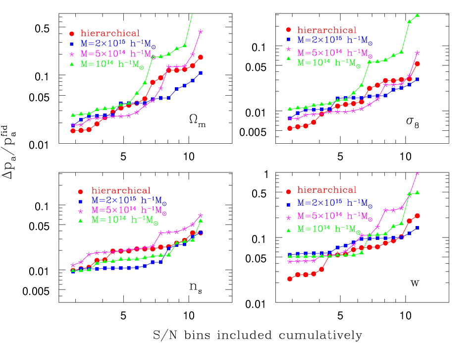
Figure 5 depicts the marginalized Fisher errors for the four cosmological parameters that we consider. The errors are fractional, i.e. the error for each parameter is divided by the fiducial value of that parameter, and cumulative, i.e. we include ${\mathcal{S}}/{\mathcal{N}}$ bins cumulatively, from the largest to the lowest. The central values of the bins are indicated on the ${\bf\hat{x}}$-axis. The symbols and colors are the same as in Figure 3. It is apparent that the hierarchical filtering performs better than the single-sized filtering, if one takes into account peaks with ${\mathcal{S}}/{\mathcal{N}}\leq 4$. The greatest improvement is for $w$: the hierarchical error is smaller by more than a factor of 2 compared to the fixed-size filtering. A smaller improvement happens also in the case of ${\sigma_{8}}$ and ${\Omega_{\rm m}}$, while the error on ${n_{\rm s}}$ seems unaffected by the filtering method, due to generally poor constraining power that peaks have on this parameter. Figure 5 reinforces the suggestion of Figure 4 that the inclusion of peaks with small ${\mathcal{S}}/{\mathcal{N}}$ improves significantly the cosmological information.

Note that for the hierarchical method we can also use aperture-mass bins to measure the peak function derivatives, the covariance matrix, and the Fisher matrix, with the mass given by Eq. (13). We obtain similar results to those presented in Figures 4, 5. The single-sized filters perform very similarly, the largest one being marginally better in the case of ${\Omega_{\rm m}}$, ${\sigma_{8}}$, and ${n_{\rm s}}$. Its diameter of 13.2 arcmin is larger than what previous studies in the literature have used: Hamana et al. (2004) had a $1$-arcmin Gaussian filter, Hennawi & Spergel (2005) employed a $\sim 5$-arcmin NFW filter, and Dietrich & Hartlap (2010) a $5.6$-arcmin one. Since the constraints from filtering with fixed sizes are so similar, we shall only show the results from the marginally-better $M=2\times 10^{15}h^{-1}M_{\odot}$ one.

In Appendix §A we examine the statistical properties of the peaks detected through the hierarchical and fixed-sized methods. We find that:

• •

  The Poisson statistic describes well the distribution of hierarchical high-${\mathcal{S}}/{\mathcal{N}}$ and high-mass peaks. The mass is defined by Eq. (13). We show that the correlation matrix of ${\mathcal{S}}/{\mathcal{N}}$-binned hierarchical peaks has strong off-diagonal contributions for the small-${\mathcal{S}}/{\mathcal{N}}$ bins, while being largely diagonal for the large-${\mathcal{S}}/{\mathcal{N}}$ bins. The same applies to the mass-binned correlation coefficient, and this behaviour is similar to that of halos, as shown in Smith & Marian (2011).

• •

  The high-${\mathcal{S}}/{\mathcal{N}}$ single-sized peaks are also reasonably described by the Poisson distribution, due to the fact that such peaks are usually quite massive and rare. The correlation matrix of these peaks seems slightly more correlated for ${\mathcal{S}}/{\mathcal{N}}\geq 7$ than the hierarchical matrix.

Lastly, in Appendix §B we investigate the dependence of the Fisher errors on the number of bins in which the ${\mathcal{S}}/{\mathcal{N}}$ interval is divided. Figure 13 suggests that all filtering methods reach the expected saturation in information if $N_{\rm bin}\leq 20$, which is why we choose $N_{\rm bin}=20$ for the results presented in this work.

We present a Fisher-matrix forecast for the 4-dimensional cosmological parameter space explored in this work. This will enable us to compare the filtering methods in a more realistic context, using marginalized errors and also cosmic microwave background (CMB) information.

For the Planck Fisher matrix, we shall assume that the CMB temperature and polarization spectra can constrain 9 parameters: the dark energy equation-of-state parameters $w_{0}$ and $w_{a}$; the density parameter for dark energy $\Omega_{\rm DE}$; the CDM and baryon density parameters scaled by the square of the dimensionless Hubble parameter $\omega_{\rm CDM}=\Omega_{\rm CDM}h^{2}$ and $\omega_{\rm b}=\Omega_{\rm b}h^{2}$ ($h=H_{0}/[100\,{\rm km\,s^{-1}\,Mpc^{-1}}]$); the primordial spectral index of scalar perturbations ${n_{\rm s}}$; the primordial amplitude of scalar perturbations $A_{s}$; the running of the spectral index $\alpha$; and the optical depth to the last scattering surface $\tau$. To compute the CMB Fisher matrix we follow Eisenstein et al. (1999):

where $\{X,Y\}\in\{{\rm TT},\,{\rm EE},\,{\rm TE},\,{\rm BB}\}$, where $C_{l,\rm TT}$ is the temperature power spectrum, $C_{l,\rm EE}$ is the E-mode polarization power spectrum, $C_{l,\rm TE}$ is the temperature-E-mode polarization cross-power spectrum, and $C_{l,\rm BB}$ is the B-mode polarization power spectrum. The assumed sky coverage is $f_{\rm sky}=0.8$ In order to make the CMB Fisher matrix compatible with our parameters, we rotate it to a new set

where for us $w_{0}=w$. We marginalize over the 5 parameters absent from our analysis.

Table 3 and Figure 6 represent the main results of this work, showing the overall improvement the hierarchical method brings over the fixed-size method after marginalization and especially after the inclusion of the CMB information. For the fixed-size method we choose the filter with $M=2\times 10^{15}\,h^{-1}M_{\odot}$, i.e. the best-performing filter among the fixed sizes that we have probed. We also show the unmarginalized errors, for a more complete picture.

Combined with the CMB, the hierarchical errors are a factor of 2 better than the single-filter method for ${\Omega_{\rm m}}$ and ${\sigma_{8}}$, and almost a factor of 3 better for $w$. For ${n_{\rm s}}$ there is no significant difference between the filtering methods. This happens because the CMB constrains the primordial power spectrum tighter than WL peak counts.

We further depict these results in Figure 6 as $2\sigma$-ellipses; the blue dashed ellipses correspond to the single-sized method, and the red solid ones to the hierarchical algorithm. Here we see again that the latter really improves the joint constraints for $\{{\sigma_{8}},{\Omega_{\rm m}},w\}$.

It is difficult to make a comparison to previous forecasts in the literature, as the probed parameter space and survey specifications are not the same, so we shall mention only two. Wang et al. (2004) presented a forecast for $\mathrm{LSST}$ in which besides WL counts they also include the cluster power spectrum, which they treat as completely independent. They consider a larger parameter space than ours, including $w_{a}$ and $\omega_{b}$, and assume $\bar{n}=65\,\mathrm{arcmin}^{-2}$ and $({\mathcal{S}}/{\mathcal{N}})_{\rm min}=4.5$. The constraints that they find when combined with $\mathit{Planck}$  priors (see Table 6 in their paper) are: $\Delta{n_{\rm s}}=0.0022,\,\Delta\Omega_{\rm DE}=0.0033,\,\Delta{\sigma_{8}}=0.0037,\Delta w=0.036$. They use a Gaussian filter of size $1$ arcmin, and their fiducial model has ${\Omega_{\rm m}}=0.27,\,{\sigma_{8}}=0.9$. The results are rather similar to ours, though their constraint of $w$ is surprisingly tight, given the sensitivity of $\Delta w$ to $({\mathcal{S}}/{\mathcal{N}})_{\rm min}$ – higher than ours – and the fact that they include $w_{a}$, known to degrade substantially the constraint on $w$.

We also make a comparison to our previous work (Marian & Bernstein, 2006), which uses the same type of normalized filter as this study. The detection threshold is 5, the projection noise is accounted for, and instead of ${n_{\rm s}}$, $w_{a}$ is considered. The fiducial values for ${\Omega_{\rm m}}$ and ${\sigma_{8}}$ are the same as in Wang et al. (2004); combining with the Planck information, we found the constraints: $\Delta{\Omega_{\rm m}}=0.005,\,\Delta{\sigma_{8}}=0.004,\Delta w=0.063$. These are in agreement with the results from the present study, given the above-mentioned differences.

We thank Gary Bernstein for his comments on the manuscript. We also thank V. Springel for making public Gadget-2 and for providing his B-FoF halo finder. LM, SH, and PS are supported by the Deutsche Forschungsgemeinschaft (DFG) through the grant MA 4967/1-1, through the Priority Programme 1177 ‘Galaxy Evolution’ (SCHN 342/6 and WH 6/3), and through the Transregio TR33 ‘The Dark Universe’. SH also acknowledges support by NSF grant number AST-0807458-002. RES was partly supported by the Swiss National Foundation under contract 200021-116696/1, the WCU grant R32-2008-000-10130-0, and the University of Zürich under contract FK UZH 57184001. RES also acknowledges support from a Marie Curie Reintegration Grant and the Alexander von Humboldt Foundation.

References

- Abate et al. (2009) Abate A., Wittman D., Margoniner V. E., Bridle S. L., Gee P., Tyson J. A., Dell’Antonio I. P., 2009, ApJ, 702, 603
- Albrecht et al. (2006) Albrecht A., Bernstein G., Cahn R., Freedman W. L., Hewitt J., Hu W., Huth J., Kamionkowski M., Kolb E. W., Knox L., Mather J. C., Staggs S., Suntzeff N. B., 2006, ArXiv Astrophysics e-prints
- Becker & Kravtsov (2011) Becker M. R., Kravtsov A. V., 2011, ApJ, 740, 25
- Bergé et al. (2008) Bergé J., Pacaud F., Réfrégier A., Massey R., Pierre M., Amara A., Birkinshaw M., Paulin-Henriksson S., Smith G. P., Willis J., 2008, MNRAS, 385, 695
- Clowe et al. (2004) Clowe D., De Lucia G., King L., 2004, MNRAS, 350, 1038
- Crocce et al. (2006) Crocce M., Pueblas S., Scoccimarro R., 2006, MNRAS, 373, 369
- Dahle (2006) Dahle H., 2006, ApJ, 653, 954
- Dietrich & Hartlap (2010) Dietrich J. P., Hartlap J., 2010, MNRAS, 402, 1049
- Eisenstein et al. (1999) Eisenstein D. J., Hu W., Tegmark M., 1999, ApJ, 518, 2
- Gao et al. (2008) Gao L., Navarro J. F., Cole S., Frenk C. S., White S. D. M., Springel V., Jenkins A., Neto A. F., 2008, MNRAS, 387, 536
- Gruen et al. (2011) Gruen D., Bernstein G. M., Lam T. Y., Seitz S., 2011, MNRAS, 416, 1392
- Hamana et al. (2004) Hamana T., Takada M., Yoshida N., 2004, MNRAS, 350, 893
- Hartlap et al. (2007) Hartlap J., Simon P., Schneider P., 2007, A&A, 464, 399
- Hennawi & Spergel (2005) Hennawi J. F., Spergel D. N., 2005, ApJ, 624, 59
- Hetterscheidt et al. (2007) Hetterscheidt M., Simon P., Schirmer M., Hildebrandt H., Schrabback T., Erben T., Schneider P., 2007, A&A, 468, 859
- Hilbert et al. (2009) Hilbert S., Hartlap J., White S. D. M., Schneider P., 2009, A&A, 499, 31
- Hilbert et al. (2007) Hilbert S., Metcalf R. B., White S. D. M., 2007, MNRAS, 382, 1494
- Hilbert et al. (2007) Hilbert S., White S. D. M., Hartlap J., Schneider P., 2007, MNRAS, 382, 121
- Hoekstra (2001) Hoekstra H., 2001, A&A, 370, 743
- Hoekstra et al. (2006) Hoekstra H., Mellier Y., van Waerbeke L., Semboloni E., Fu L., Hudson M. J., Parker L. C., Tereno I., Benabed K., 2006, ApJ, 647, 116
- Israel et al. (2010) Israel H., Erben T., Reiprich T. H., Vikhlinin A., Hildebrandt H., Hudson D. S., McLeod B. A., Sarazin C. L., Schneider P., Zhang Y.-Y., 2010, A&A, 520, A58+
- Jarvis et al. (2003) Jarvis M., Bernstein G. M., Fischer P., Smith D., Jain B., Tyson J. A., Wittman D., 2003, Astronomical Journal, 125, 1014
- Jarvis et al. (2006) Jarvis M., Jain B., Bernstein G., Dolney D., 2006, ApJ, 644, 71
- Komatsu et al. (2009) Komatsu E., Dunkley J., The WMAP Team 2009, ApJS, 180, 330
- Kratochvil et al. (2010) Kratochvil J. M., Haiman Z., May M., 2010, PRD, 81, 043519
- Kratochvil et al. (2011) Kratochvil J. M., Lim E. A., Wang S., Haiman Z., May M., Huffenberger K., 2011, ArXiv e-prints
- Kuijken (2010) Kuijken K., 2010, in D. L. Block, K. C. Freeman, & I. Puerari ed., Galaxies and their Masks Dark Haloes as Seen with Gravitational Lensing. pp 361–+
- LSST Science Collaborations et al. (2009) LSST Science Collaborations Abell P. A., Allison J., Anderson S. F., Andrew J. R., Angel J. R. P., Armus L., Arnett D., Asztalos S. J., Axelrod T. S., et al. 2009, ArXiv e-prints
- Marian & Bernstein (2006) Marian L., Bernstein G. M., 2006, PRD, 73, 123525
- Marian et al. (2011) Marian L., Hilbert S., Smith R. E., Schneider P., Desjacques V., 2011, ApJL, 728, L13+
- Marian et al. (2009) Marian L., Smith R. E., Bernstein G. M., 2009, ApJL, 698, L33
- Marian et al. (2010) Marian L., Smith R. E., Bernstein G. M., 2010, ApJ, 709, 286
- Maturi et al. (2010) Maturi M., Angrick C., Pace F., Bartelmann M., 2010, A&A, 519, A23+
- Maturi et al. (2005) Maturi M., Meneghetti M., Bartelmann M., Dolag K., Moscardini L., 2005, A&A, 442, 851
- Metzler et al. (2001) Metzler C. A., White M., Loken C., 2001, ApJ, 547, 560
- Navarro et al. (1997) Navarro J. F., Frenk C. S., White S. D. M., 1997, ApJ, 490, 493
- Okabe et al. (2010) Okabe N., Takada M., Umetsu K., Futamase T., Smith G. P., 2010, Publications of the Astronomical Society of Japan, 62, 811
- Pires et al. (2009) Pires S., Starck J.-L., Amara A., Réfrégier A., Teyssier R., 2009, A&A, 505, 969
- Schirmer et al. (2007) Schirmer M., Erben T., Hetterscheidt M., Schneider P., 2007, A&A, 462, 875
- Schneider (1996) Schneider P., 1996, MNRAS, 283, 837
- Schneider et al. (1998) Schneider P., van Waerbeke L., Jain B., Kruse G., 1998, MNRAS, 296, 873
- Scoccimarro (1998) Scoccimarro R., 1998, MNRAS, 299, 1097
- Seljak & Zaldarriaga (1996) Seljak U., Zaldarriaga M., 1996, ApJ, 469, 437
- Semboloni et al. (2006) Semboloni E., Mellier Y., van Waerbeke L., Hoekstra H., Tereno I., Benabed K., Gwyn S. D. J., Fu L., Hudson M. J., Maoli R., Parker L. C., 2006, A&A, 452, 51
- Sheth & Tormen (1999) Sheth R. K., Tormen G., 1999, MNRAS, 308, 119
- Smith (2009) Smith R. E., 2009, MNRAS, 400, 851
- Smith & Marian (2011) Smith R. E., Marian L., 2011, MNRAS, 418, 729
- Smith & Watts (2005) Smith R. E., Watts P. I. R., 2005, MNRAS, 360, 203
- Springel (2005) Springel V., 2005, MNRAS, 364, 1105
- Tang & Fan (2005) Tang J. Y., Fan Z. H., 2005, ApJ, 635, 60
- Tegmark et al. (1997) Tegmark M., Taylor A. N., Heavens A. F., 1997, ApJ, 480, 22
- The Dark Energy Survey Collaboration (2005) The Dark Energy Survey Collaboration 2005, ArXiv Astrophysics e-prints, pp astro–ph/0510346
- The Euclid Collaboration (2011) The Euclid Collaboration 2011, arXiv:astro-ph/1110.3193
- Wang et al. (2004) Wang S., Khoury J., Haiman Z., May M., 2004, PRD, 70, 123008
- Yang et al. (2011) Yang X., Kratochvil J. M., Wang S., Lim E. A., Haiman Z., May M., 2011, PRD, 84, 043529
Appendix A The correlation coefficient of the peak counts
For a covariance matrix , the correlation coefficient is defined by