Charles University in Prague
Faculty of Mathematics and Physics
DOCTORAL THESIS
![[Uncaptioned image]](1110.4553v1/logo.png)
Ondřej Kopáček
Transition from regular to chaotic motion
in black hole magnetospheres
Astronomical Institute of the Academy of Sciences
of the Czech Republic
Supervisor: doc. RNDr. Vladimír Karas, DrSc.
Prague 2011
The thesis summarizes the results of the research conducted during the doctoral studies of the branch Theoretical physics, Astronomy and Astrophysics at the Faculty of Mathematics and Physics of Charles University in Prague during the years 2007-2011.
Student
Mgr. Ondřej Kopáček
Supervisor
doc. RNDr. Vladimír Karas, DrSc.
Astronomical Institute of the Academy of Sciences of the Czech Republic
Affiliation
Astronomical Institute of the Academy of Sciences of the Czech Republic
Boční II 1401/1a, 14131 Prague
Referees
Prof. Luciano Rezzolla, Ph.D.
Albert Einstein Institut, Potsdam
Prof. RNDr. Petr Kulhánek, CSc.
FEL ČVUT, Prague
The thesis was successfully defended on 14 September 2011 in Prague before the committee of the study branch 4F1 (Theoretical physics, Astronomy and Astrophysics).
Acknowledgements
I would like to thank my supervisor, Dr. Vladimír Karas, for the patient guidance, encouragement and advice he has provided throughout my doctoral studies.
I declare that I carried out this doctoral thesis independently, and only with the cited sources, literature and other professional sources.
I understand that my work relates to the rights and obligations under the Act No. 121/2000 Coll., the Copyright Act, as amended, in particular the fact that the Charles University in Prague has the right to conclude a license agreement on the use of this work as a school work pursuant to Section 60 paragraph 1 of the Copyright Act.
Název práce: Regulární a chaotické pohyby v magnetosféře černých děr
Autor: Ondřej Kopáček
Katedra (ústav): Astronomický ústav Univerzity Karlovy
Školicí pracoviště: Astronomický ústav Akademie věd České republiky
Vedoucí doktorské práce: doc. RNDr. Vladimír Karas, DrSc., Astronomický ústav Akademie věd České republiky, Praha
Abstrakt: Působení silné gravitace v okolí černých děr může vést k urychlení hmoty. V této práci zkoumáme vlastnosti systému tvořeného rotující černou dírou ve velkorozměrovém uspořádaném magnetickém poli. Nabité částice v blízkosti horizontu jsou kromě silné gravitace ovlivňovány magnetickým polem a indukovaným polem elektrickým. Oproti již dříve v literatuře diskutovaným situacím přidáváme některá významná zobecnění. Magnetické pole v našem případě nemusí být koaxiální s rotační osou černé díry, takže systém ztrácí osovou symetrii. Kromě toho předpokládáme translační pohyb černé díry s obecným směrem i rychlostí. Ukážeme, že díky tomu dochází k novým efektům. V komplikované struktuře výsledného magnetického pole pozorujeme v ergosféře jeho rychlé prostorové změny provázené vznikem nulových bodů, které dokazují, že gravitační působení rotujícího zdroje může podněcovat rekonekci magnetických siločar. Dále zkoumáme dynamické vlastnosti nabitých částic vystavených působení tohoto typu polí. Především se zajímáme o přechody mezi regulárním režimem a deterministickým chaosem, ke kterým dochází v závislosti na volbě parametrů. Při numerickém zkoumání částicové dynamiky aplikujeme v kontextu obecné relativity zatím nepoužitou metodu rekurenční analýzy.
Klíčová slova: obecná relativita, kompaktní tělesa, astrofyzikální koróna, deterministický chaos
Title: Transition from regular to chaotic motion in black hole magnetospheres
Author: Ondřej Kopáček
Department: Astronomical Institute of Charles University
Affiliation: Astronomical Institute of Academy of Sciences of the Czech Republic
Supervisor: doc. RNDr. Vladimír Karas, DrSc., Astronomical Institute of the Academy of Sciences of the Czech Republic, Prague
Abstract: Cosmic black holes can act as agents of particle acceleration. We study properties of a system consisting of a rotating black hole immersed in a large-scale organized magnetic field. Electrically charged particles in the immediate neighborhood of the horizon are influenced by strong gravity acting together with magnetic and induced electric components. We relax several constraints which were often imposed in previous works: the magnetic field does not have to share a common symmetry axis with the spin of the black hole but they can be inclined with respect to each other, thus violating the axial symmetry. Also, the black hole does not have to remain at rest but it can instead perform fast translational motion together with rotation. We demonstrate that the generalization brings new effects. Starting from uniform electro-vacuum fields in the curved spacetime, we find separatrices and identify magnetic neutral points forming in certain circumstances. We suggest that these structures can represent signatures of magnetic reconnection triggered by frame-dragging effects in the ergosphere. We further investigate the motion of charged particles in these black hole magnetospheres. We concentrate on the transition from the regular motion to chaos, and in this context we explore the characteristics of chaos in relativity. For the first time, we apply recurrence plots as a suitable technique to quantify the degree of chaoticness near a black hole.
Keywords: general relativity, compact objects, astrophysical coronae, deterministic chaos
Chapter 1 Introduction
1.1 Astrophysical black holes
Nowadays it is a consensus that black holes are a vivid part of physical reality. Astrophysicist’s attitude toward the possibility of a real existence of completely gravitationally collapsed bodies, i.e. black holes (BHs), has undergone profound changes since 1935 when sir Eddington commented recent theoretical results of Chandrasekhar (1935), suggesting that black hole could be the endpoint of star evolution, by these words: “I think there should be a law of Nature to prevent a star from behaving in this absurd way”. At present, due to discoveries and observations made in recent decades, it seems highly probable that there is actually no such power which would save a heavy star from collapsing into the black hole.
Until the late 1960’s there had not been much progress made in this field. Although Karl Schwarzschild had given an exact solution to Einstein’s equations for a spherically symmetrical source (Swcharzschild black hole in the case of collapsed body) already in 1916 (just one year after publishing the theory of relativity), it was not believed that such objects really exist. Almost a half century later, Kerr (1963) gave a new exact solution to Einstein’s field equations describing the geometry around a rotating compact object, which naturally appears to be more relevant in astrophysical context than prior non-rotating Schwarzschild solution. But this progress still would not become a concern of astrophysicists unless there had not been made important observational discoveries during 1960’s.
Astronomers discovered sources of radio waves with highly redshifted (with redshift factor ) spectrum (Schmidt, 1963) which proved them (according to Hubble’s law) to be very distant from us ( ). Combined with observed visual magnitude of these objects – called quasars (quasi-stellar radio sources) – there comes a conclusion of their huge power output of about 100 times that of the total luminosity of average galaxy (). Quasars also appeared to emit significantly in X-ray and even in gamma part of the spectrum.
Quasars were not the only peculiar objects observed during those decades. According to the type of their spectrum and luminosity time dependence of those “new” objects they were classified as Seyfert galaxies (being observed and studied since the 1940’s actually), blazars, or radio galaxies (RGs) with all of them consisting of further subclasses. They are all characterized by extraordinarily high luminosity coming from a small volume (). As there is no consistent way to explain the mechanism of those energy sources conventionally (i.e. regarding stars and therein running nuclear synthesis as the most efficient energy source in the universe), attention was turned to hypothesis employing strong gravitational fields considering compact objects and subsequently the black holes. Now it is generally believed that above mentioned phenomenons are of the same origin which was given the name active galactic nuclei (AGN). Galaxies with active galactic nuclei and subsequently also those with non-active nuclei are suspected of hosting a supermassive black hole (MBH) of in their centres, e.g. M87 – AGN of or Sagittarius A* – nonactive nucleus of our Galaxy – with (Genzel et al., 2010).

The main reason for such an assumption is that it provides a clarification of the observed luminosity of active galaxies. When the Kerr black hole is employed to model the properties of AGN we conclude that the matter accreted from its vicinity would form an accretion disk which becomes heated by accretion process and subsequently emits radiation of various types (depending on temperature and many other properties of the disk). Doing so there could be as much as (Misner et al. (1973) p. 885) of accreted material rest mass turned into emitted radiation which is considerably more than in the case of thermonuclear synthesis of helium ( of the rest mass).
Whether we regard observed AGN as quasar, radio galaxy, blazar or Seyfert galaxy depends mostly on the spatial orientation of the surrounding galaxy which acts as the shield for some parts of the spectrum while being a source in some other parts (see Urry & Padovani, 1995, for a review of unified schemes of radio sources).
Tolman-Oppenheimer-Volkoff (TOV) limit sets the upper bound to the mass of neutron star (Oppenheimer & Volkoff, 1939). Today’s estimates of the value of TOV limit range among (Lattimer & Prakash, 2004) and the uncertainty is due to unknown equation of state. Pressure of degenerate neutron gas in the neutron star reaching this limit cannot oppose gravitational pressure and inevitably collapses into the black hole (while collapse is being accompanied with gamma ray burst, GRB). Stellar mass black hole () should thus represent the final state of stellar evolution of every heavier star. To be observed it needs to be a part of the binary system. Under certain circumstances black hole accretes matter from its companion star (flowing via Lagrange point when boundaries of a Roche lobe are exceeded). Similarly like in the supermassive black hole case there establishes accretion disk emitting in X-ray part of the spectrum. Due to recent observation from the satellites Chandra and XMM-Newton equipped with high resolution X-ray detectors we now have many stellar mass black hole candidates in our Galaxy (e.g. Cygnus X-1). The key to distinguish accretion disk of a compact object (typically neutron star) from the one surrounding the black hole is the nonexistence of the surface in the black hole case. Thus irregular flares of gamma rays accompanying thermonuclear reaction of accreted material on the compact object surface are not detected.
Intermediate-mass black holes (IMBHs) are those with . Existence of IMBHs is still uncertain although a number of candidates was identified. IMBH might be possibly formed in globular star clusters (Maccarone et al., 2007). Ultra-luminous X-ray sources (ULXs) in close galaxies are suspected to be powered by IMBH. An ULX source HLX1 located on the edge of spiral galaxy ESO243-49 was claimed (Farrell et al., 2009) to host an IMBH of over , though the interpretation was recently disputed by Soria et al. (2011). A stellar complex IRS 13E residing close to our galactic center Sagittarius A* is yet another candidate for the IMBH system (Schoedel et al., 2005).
Primordial black holes (PBHs) are hypothetical objects whose origin differs fundamentally from all above mentioned types. They have not been established by gravitational collapse of stars or other astronomical bodies since they might have been born from density fluctuation during early stages of the evolution of the Universe. On the theoretical grounds it has been argued (Carr & Hawking, 1974) that PBHs of mass from upwards might exist in the present Universe. Updated constraints on PBHs were given recently by Carr et al. (2010). Primordial black holes could be detected due to the Hawking radiation which black holes emit according to the quantum relativity (Page, 1976).
Hawking radiation has ordinary thermal spectra and energy it radiates away goes on account of the mass – the black hole evaporates. Predicted evaporation times for stellar mass black holes exceed present age of the universe by many orders but for primordial black holes with the mass evaporation time approaches its current age. Rate of evaporation escalates as the mass decreases (power output ). Endpoint of the primordial black hole existence should thus be explosive (Hawking, 1974) and is believed to be accompanied with loud GRB. Search for these GRB signatures is one of the key scientific objectives of current mission of Fermi Gamma-ray Space Telescope which is operating since 2008.

1.2 Magnetic field: trigger for accretion and outflow
Recent observations of microquasars, pulsars, gamma-ray bursts indicate that the astrophysical jets play an important role everywhere (not only in the case of AGNs). There is plenty of observational evidence suggesting that the initial acceleration of jets takes place very near black holes (or other compact object) and proceeds via electromagnetic forces. Jets and accretion disks in the vicinity of compact objects probably create symbiotic magnetically driven system (Falcke & Biermann, 1995, e.g.).
The current promising model of the dynamics (i.e. launching, accelerating and collimating) of the astrophysical jets is based on the magnetohydrodynamics (MHD). The results of the simulations employing general relativistic MHD equations (Krolik & Hawley, 2010) correlate with observations of M87 (Junor et al., 1999) where the formation and the collimation of the jet were analyzed.
Moreover, the 3D relativistic MHD simulations carried out by Hawley & Krolik (2006) demonstrate clearly the essential role which the accretion disk’s coronae play in the collimation and acceleration of the jet. Indeed the dominant force accelerating the matter outward in a given numerical model originates from the coronal pressure. Regions above and below the equatorial plane become dominated by the magnetic pressure and large-scale magnetic fields may also develop by the dynamo action.
Recent numerical relativistic study by Rezzolla et al. (2011) reveals the formation of ordered jet-like structure of ultrastrong magnetic field in the merger of binary neutron stars. Such system thus might serve as an astrophysical engine for observed short gamma ray bursts.
In accretion models the magnetic field was also employed – the so called magnetorotational instability (MRI) must operate in accretion disc, generating the effective viscosity necessary for the accretion process (Balbus, 1991). Magnetic reconnection is likely to be responsible for rapid flares, which are observed in X-rays. Finally, Faraday rotation measurements suggest that tangled magnetic fields are present in jets (Begelman et al., 1984).
Observations of the Galactic Center (GC) reveal the presence of another remarkable large-scale magnetic structure – nonthermal filaments (NTFs). NTFs cross the Galactic plane and their length reaches tens of parsecs while they are only tenths of parsec wide. The strength of the magnetic field within the NTF may approach while the typical interstellar value is (LaRosa et al., 2004). Initially, it was thought that NTFs trace the pervasive poloidal magnetic field present throughout the GC (Morris, 1990). Later, however, it became apparent that the structure of the magnetic field in the central region of the Galaxy is more complex (Ferrière, 2010). See fig. 1.3 for the snapshot of the GC at which shows the NTFs clearly.

Overall it is quite likely that electromagnetic mechanisms play a major role and operate both near supermassive black holes in quasars as well as stellar-mass black holes and neutron stars in accreting binary systems (see figures 1.1 and 1.2). Besides that a faint magnetic field is present throughout the interstellar medium, being locally intensified in NTFs.
Electro-vacuum fields
The survey of the vacuum electromagnetic (EM) fields may be regarded as the fundamental starting point in studying the dynamics of astrophysical plasma. If the examination of the fields itselves represents the initial step in a given direction, at succeeding stage we would consider the motion of a non-interacting test particles exposed to these fields. In this work we will be dealing with both issues. Structure of a particular astrophysically motivated EM field emerging in the vicinity of rotating black hole will be studied in detail. Subsequently we shall discuss the motion of charged particles exposed to the field representing a special case of a general solution explored before. Primarily we concern ourselves with the stable orbits occupying off-equatorial potential lobes. Particles on these orbits are relevant for the description of astrophysical corona comprising of diluted plasma residing outside the equatorial plane in the inner parts of accreting black hole systems.
Gaseous corona is supposed to play a key role in the formation of observed X-ray spectra of both active galactic nuclei (AGNs) and microquasars (Done, 2001). Power law component of the spectra is believed to result from the inverse Compton scattering of the thermal photons emitted in the inner parts of the disk. Relativistic electrons residing in the corona serve as a scatterers in this process. Their dynamic properties (e.g. resonances) thus shall have imprint on the observed spectra.
The role of magnetic fields near strongly gravitating objects has been subject of many investigations (Punsly, 2008, e.g.). They are relevant for accretion disks that may be embedded in large-scale magnetic fields, for example when the accretion flow penetrates close to a neutron star (Lipunov et al., 1992; Mestel, 1999). Outside the main body of the accretion disk, i.e. above and below the equatorial plane, the accreted material forms a highly diluted environment, a corona, where the density of matter is low and the mean free path of particles is large in comparison with the characteristic length-scale, i.e. the gravitational radius of the central body, km, where is the central mass. The origin of the coronal flows and the relevant processes governing their structure are still unclear. In this context we discuss motion of electrically charged particles outside the equatorial plane.
Regular and chaotic dynamics
Accretion onto black holes and compact stars brings material in a zone of strong gravitational and electromagnetic fields. We study dynamical properties of motion of electrically charged particles forming a highly diluted medium (a corona) in the regime of strong gravity and large-scale (ordered) magnetic field.
We start our discussion from a system that allows regular motion, then we focus on the onset of chaos. To this end, we investigate the case of a rotating black hole immersed in a weak, asymptotically uniform magnetic field. We also consider a magnetic star, approximated by the Schwarzschild metric and a test magnetic field of a rotating dipole. These are two model examples of systems permitting energetically bound, off-equatorial motion of matter confined to the halo lobes that encircle the central body. Our approach allows us to address the question of whether the spin parameter of the black hole plays any major role in determining the degree of the chaoticness.
The both dynamic systems may be regarded as different instances of the originally integrable systems which were perturbed by the electromagnetic test field. Complete integrability of geodesic motion of a free particle in Schwarzschild spacetime is easy to verify (Misner et al., 1973). To some surprise it was later found that also free particle motion in Kerr spacetime and even the charged particle motion in Kerr-Newman is completely integrable (Carter, 1968) since separation of the equations of motion is possible as there exists additional integral of motion – Carter’s constant . Trajectories found in such a systems are merely regular.
In the non-integrable system, however, both regular and chaotic trajectories may coexist in the phase space. Standard method of a qualitative survey of the non-linear dynamics is based on the construction of Poincaré surfaces of section which allow to visually discriminate between the chaotic and regular regime of motion.
On the other hand quantifying the chaos by Lyapunov characteristic exponents (LCEs), as its standard and commonly used indicator, becomes problematic in the general relativity (GR) since LCEs are not invariant under the coordinate transformations. Besides that the usual method of computing LCEs involves evaluation of the distances between the neighboring trajectories which becomes intricate in GR. Although there are operational workabouts to partially overcome these difficulties (Wu & Huang, 2003, e.g.) the need for a consistent treatment is apparent. Perhaps the geometrical approach suggested recently by Stachowiak & Szydlowski (2010) could eventually provide a covariant method of the evaluation of the Lyapunov spectra in GR.
In this context we adopt a different tool to investigate the dynamic system – Recurrence Analysis (Marwan et al., 2007). To characterize the motion, we construct the Recurrence Plots (RPs) and we compare them with Poincaré surfaces of section. We describe the Recurrence Plots in terms of the Recurrence Quantification Analysis (RQA), which allows us to identify the transition between different dynamical regimes. We demonstrate that this new technique is able to detect the chaos onset very efficiently, and to provide its quantitative measure. The chaos typically occurs when the conserved energy is raised to a sufficiently high level that allows the particles to traverse the equatorial plane. We find that the role of the black-hole spin in setting the chaos is more complicated than initially thought.
1.3 Structure of Thesis
The thesis is organized as follows. Most of its contents are contained in chap. 2. We begin with technical preliminaries, namely in sec. 2.2 we introduce several alternative definitions of electric and magnetic vector fields. In sec. 2.3 we give explicitly the components of the electromagnetic tensor describing the field around the Kerr black hole drifting in the arbitrary direction through the asymptotically homogeneous magnetic field which is generally inclined with respect to the rotation axis of the BH. Choice of the observer’s frame is discussed in sec. 2.4. Structure of the both electric and magnetic fields is explored in detail in sec. 2.5. First in sec. 2.5.1 we revisit the issue of the magnetic expulsion (Meissner effect) which is present in the case of aligned field. Subsequently we study field structures in the case of inclined field. Finally, in sec. 2.5.2 we introduce a drift of the black hole and explore the both electric and magnetic fields emerging in this general setup.
In the remaining part of the chap. 2 we shall deal with the dynamics of the charged test particles exposed to the test fields analyzed in the previous sections. In sec. 2.7 we review the equations of particle motion, which we then integrate to obtain trajectories. In sec. 2.8 we introduce the basic properties of Recurrence Plots. Sec. 2.9 analyses the motion around a Kerr black hole endowed with a uniform magnetic test field. We employ Poincaré surfaces of section and Recurrence Plots. The two approaches allow us to show the onset of chaos in different, complementary ways. We examine the motion in off-equatorial lobes, pay special attention to the spin dependence of the stability of motion, and we notice the emergence of ‘potential valleys’ that allow the particles to escape from the equatorial plane along a narrow collimated corridor. Analysis of the off-equatorial motion around a magnetic star is presented in sec. 2.10. We consider a dipole-type magnetic field, which sets different limits on the off-equatorial range of allowed motion of charged particles. It also defines different regimes of chaoticness in the comparison with the uniform magnetic field.
Finally, results of the analysis are summarized in chap. 3. Chapter 4 represents a brief outlook to the future as it specifies several topics suggesting the direction in which our research could continue.
In Appendix A we list conversion factors between SI and geometrized units. Scaling of the quantities by the central mass is also discussed. Appendix B gives detailed comparison of numerical integrators applicable to our system. Benefits of symplectic routines are discussed therein. In Appendix C we introduce our program tool vfexplorer2 which provides a simple graphic user interface (GUI) for the effective exploration of a complex vector fields.
Most of the scientific contents presented in the Thesis were published in the papers Kopáček et al. (2010a) and Karas & Kopáček (2009). Investigation of the particle motion in the astrophysical corona was preceded by the study of the topology of off-equatorial potential lobes performed by Kovář et al. (2010). Discussion of the charged particle motion in such lobes was also a subject of the contribution Kopáček et al. (2010b). Initial steps of the investigation of electromagnetic fields around drifting Kerr black hole were described by Kopáček (2008).
At different phases of my doctoral studies I took part in several research projects. Namely I acknowledge support from the doctoral student program of the Czech Science Foundation (project No. 205/09/H033), Plan for European Cooperating States of the European Space Agency (ESA PECS 98040) and two projects of the Grant Agency of Charles University (GAUK 119210/2010 and SVV-263301).
Chapter 2 Regular and chaotic motion in black hole magnetospheres
2.1 Electromagnetic field around drifting Kerr black hole
In this section we construct a test field solution describing the electromagnetic field around a Kerr black hole which is drifting in an arbitrary direction with respect to the asymptotically uniform magnetic field with the general orientation with respect to the rotation axis. Definition of the electric and magnetic field intensities is discussed as well as the choice of the physical observer. Structure of the field is explored in detail.
Electromagnetic (EM) test field solutions of Maxwell equations in curved spacetime play an important role in astrophysics since we can usually suppose that astrophysically relevant EM fields are weak enough, so that their influence upon background geometry may be neglected.
We are interested in the solutions describing an originally uniform magnetic field under the influence of the Kerr black hole. Since the Kerr metric is asymptotically flat, this EM field reduces to the original homogeneous magnetic field in the asymptotic region. First such a test field solution was given by Wald (1974) for the special case of perfect alignment of the asymptotically uniform magnetic field with the symmetry axis. Using a different approach of Newman Penrose formalism a more general solution for an arbitrary orientation of the asymptotic field was inferred by Bičák & Dvořák (1980). We use their solution to construct the EM field around the Kerr black hole which is drifting through the asymptotically uniform magnetic field.
Such generalized setup shall represent an astrophysically relevant model. In the actual accreting BH system the misaligned ordered field may arise if the accretion disk is inclined with respect to the rotation axis of the BH and the Bardeen-Petterson effect does not operate to align the axes. Such misaligned accretion was observed in some numerical simulations (Rockefeller et al., 2005, e.g.). A possible scenario how the BH could receive substantial velocity with respect to its accretion disk is suggested by the simulations of a merger process (Rezzolla, 2009; Gonzáles et al., 2007, e.g.).
In the context of black hole mergers Lyutikov (2011) recently studied electrodynamic properties of the simplified model consisting of the Schwarzschild black hole in the uniform transversal motion with respect to the homogeneous magnetic field. The author considers the interaction of the field with the plasma generated from the pair production due to the vacuum breakdown. Analyzing the resulting situation in the force-free approximation, Lyutikov concludes that observed electrodynamic properties resemble in many aspects the pulsar magnetosphere.
2.2 Lines of force
Kerr metric in Boyer-Lindquist coordinates may be expressed as follows (Misner et al., 1973):
| (2.1) |
where
| (2.2) |
We stress that geometrized units are used throughout the text. See Appendix A for details.
For the sake of reference it might be useful to list both covariant and contravariant components of the Kerr metric explicitly
| (2.3) | |||
| (2.4) | |||
denoting . Following relation proved useful in the calculations: .
Radial metric component and contravariant components , and are singular at which defines the outer (+) and the inner (-) horizon of the black hole. By querying the curvature scalars one finds that the singularities present at are purely coordinate singularities rather than physical ones. Both horizons merge at in the case of extreme Kerr black hole . For the horizon disappears and the central singularity becomes naked. In the following, however, we will be concerned with the cases only.
Dragging of the inertial frames caused by the rotation of the source may be characterized by the quantity . Coordinate angular velocity (“angular velocity as measured at infinity“) of the observer freely falling from the rest at infinity reads (see eq. 2.53).
In the classical electrodynamics we spontaneously define electric and magnetic lines of force as a field lines of three-vectors and which form a solution of Maxwell equations for a given problem. Definition condition of the field line parametrized by the parameter is such that its tangent vector is at each point parallel to the vector field itself. Thus for (e.g. electric) lines of force we obtain equation
| (2.5) |
where stands for the ordinary cross product of two vectors.
If we recall Lorentz relation specifying the force felt by a particle with electric test charge and hypothetical magnetic monopole test charge moving with the velocity in the external fields ,
| (2.6) |
we conclude that in a given reference frame we can identify the electric intensity with the force felt by the unit electric charge and magnetic induction with the force felt by the unit magnetic monopole charge provided that these charges are static in a given reference frame.
In the covariant language of general relativity the Lorentz force felt by the test particle of mass and the electric charge or the magnetic monopole charge is expressed as follows:
| (2.7) | ||||
| (2.8) |
where stands for the proper time, a is particle’s four-acceleration, u its four-velocity and are Christoffel symbols. is electromagnetic tensor and its dual.
In the close analogy with the classical case it appears natural to define coordinate components of magnetic and electric fields as follows (Hanni & Ruffini, 1973)
| (2.9) |
However, the demand on the test charge to be static in a given reference frame, i.e. to have 4-velocity of a form , becomes highly problematic when dealing with the non-static geometry of the Kerr spacetime. It is well known that in this case no physical observer may remain static inside the ergosphere whose boundary is defined by
| (2.10) |
Since the region near the horizon is typically of a big interest when investigating the effects of a strong gravity we do not content us with being limited to the region outside the ergosphere. To this end we generalize the above definition eq. (2.9) in such a way that we allow general four-velocity of the test charge . In the classical analogy this would mean not insisting on when defining the vector fields and using the classical form of the Lorentz force equation (2.6). Nevertheless all the cases we shall discuss actually have therefore we may write explicitely
| (2.11) | ||||
| (2.12) | ||||
| (2.13) |
Equation for the lines of force eq. (2.5) takes following form in the poloidal plane: and similarly in the equatorial plane: . To obtain analogical expressions for the components of electric field , , we just need to omit the minus sign at the beginning of each term and replace components with in eqs. (2.11)–(2.13).
Another issue connected with the definition (2.9) is a question of the normalization of the basis vectors. We notice that components of magnetic and electric fields and are provided in the canonical basis of Boyer-Lindquist coordinates, namely in the basis of vectors , , , which are not normalized. This problem may be seemingly easily overcome by expressing ”physical components” of the fields111footnotetext: The adjective physical is sometimes used to refer to the quantities measured in the frame attached to a given physical observer. We stress that our usage of the term differs as our physical components are expressed in the coordinate frame. (Hanni & Ruffini, 1973) as follows
| (2.14) | ||||
| (2.15) | ||||
| (2.16) |
and analogically for physical components of electric field .
However, in the case of Boyer-Lindquist coordinate system which is singular at the horizon (namely the radial metric component diverges here) using above defined physical components turns out to be a controversial choice since it introduces this divergence directly into the radial component of electric and magnetic fields.
To fix this problem we suggest to define “renormalized components“ of the fields as follows
| (2.17) | ||||
| (2.18) | ||||
| (2.19) |
where , , are ordinary Lamé coefficients of spherical coordinates in flat space. Correspondence between physical and renormalized components lies in the asymptotic region where they become identical since the Kerr spacetime is asymptotically flat and Boyer-Lindquist coordinates asymptotically turn into spherical coordinates describing the spatial part of Minkowskian spacetime. Explicitly given the asymptotic behaviour of the metric coefficients is , and and .
Going even further in ”operational flattening“ of the curved background one could eventually identify the components of magnetic and electric fields directly with the components of the electromagnetic tensor . Such an identification is fully justified in any local Lorentz frame where takes the form given by eq. (2.25). Nevertheless although the asymptotics of Kerr background is flat, its Boyer-Lindquist coordinate basis -forms are not normalized and normalization factors , and must be used accordingly. We define asymptotically motivated (AMO) components of the fields
| (2.20) | ||||
| (2.21) | ||||
| (2.22) |
AMO components asymptotically coincide with the physical and renormalized components provided that the test charge is static. Although AMO components do not allow for a direct physical interpretation when applied outside the asymptotic region, it may still be useful to explore them since they do not employ any particular observer (four-velocity of a test charge) in their definition and therefore it may be easier to acquire intuitive insight into the nature of a given EM field.
Nevertheless a consistent way to define the electric and magnetic fields should provide obvious physical interpretation of the observables measured by a certain physical observer at any distance from the center. We let such an observer with four-velocity equipped with the orthonormal tetrad measure the Lorentz force of eq. (2.9) using his tetrad basis. Tetrad components of the vector fields determining desired lines of force are given as the spatial part of the projection
| (2.23) | ||||
| (2.24) |
where are 1-forms dual to the tetrad vectors . Lowering/raising of the spatial tetrad indices does not matter since the tetrad is supposed to be orthonormal: .
For the sake of the future reference we review both tetrad components of EM tensor and its dual . We remind that such an interpretation of these tensors is possible only in any local Lorentz frame which may be attached to any physical observer, not necessarily inertial. Magnetic and electric test charges which are used to measure the fields are at rest in this frame.
| (2.25) |
| (2.26) |
Several ways to define electric and magnetic field have been described in this section. Coordinate components of the Lorentz force felt by the unit electric/magnetic test charge (eq. 2.9) provide a natural generalization of the classical definition. In the case of the Kerr background, however, we cannot insist upon the usage of the static test charges in the definition as no static observers may penetrate inside the ergosphere. Since the structure of the fields in the vicinity of the horizon is usually of the utmost interest we have assumed more general four-velocity of the test charge in the form . The Lorentz force may be projected onto the tetrad basis attached to the test charge.
Nevertheless if we remain in the Boyer-Lindquist coordinate basis we note that the fields do not come with the proper dimension because the coordinate basis vectors are not normalized. To correct this in a rigorous manner we define physical components of the fields by eqs. (2.14)–(2.16). It appears, however, that this definition amplifies the effect of the coordinate singularity at the horizon. Thus we suggested to define renormalized components (eqs. 2.17–2.19) as an useful approximation which is less problematic near the horizon. Far more approximative (in the sense of treating the curved background as flat) are asymptotically motivated AMO components (eqs. 2.20–2.22) which in fact map onto the flat surface directly. Brief discussion regarding the definition of the lines of force of electric and magnetic fields was also held by Bičák & Dvořák (1980).
2.3 Electromagnetic field
Stationary and axisymmetric test field solutions to the Maxwell equations on the Kerr background traditionally attract attention by both relativistic theoreticians and astrophysicists. The latter are usually concerned with the solutions describing some potentially realistic electrodynamic scenario. In particular we mention test fields of axisymmetric current loops (Petterson, 1975; Moss, 2011) and uniform magnetic field (Wald, 1974; Bičák & Dvořák, 1976).
We start out from the describing the test field with asymptotic form of a general (i.e. not necessarily parallel) uniform magnetic field given by Bičák & Janiš (1985). Due to the axial symmetry of Kerr space-time only two components of asymptotic field were considered in that paper without any loss of generality (asymptotic components (parallel) and (equatorial) to be specific). We rewrite components of EM tensor (Bičák & Janiš, 1985, eq. (A3) of) denoting , and splitting the result into two parts according to the asymptotic component. We obtain the asymptotically perpendicular part of the field:
| (2.27) | ||||
and the part which approaches uniform field aligned along the axis:
| (2.28) | ||||
where we use the azimuthal coordinate of Kerr ingoing coordinates, which is related to Boyer–Lindquist coordinates as follows:
| (2.29) |
with denoting the outer and the inner horizon. We notice that .
As we shall introduce a drift of the black hole in the general direction we lose axial symmetry and need to consider all spatial components of the asymptotic magnetic field. We obtain (which may only appear due to nonzero drift) by rotating along the -axis by angle - i.e. which only causes and .
Since the drift shall induce uniform electric field in the asymptotic region we need to have appropriate handy. We get them easily by performing dual transformation of . Dual transformation is carried out as follows:
| (2.30) |
where is the Levi-Civita tensor whose components are given as:
| (2.31) |
with denoting completely antisymmetric symbol. Determinant of the Kerr metric is .
Performing the dual transformation we immediately obtain EM tensors with desired asymptotics of uniform electric field:
| (2.32) |
In the explicit form we get:
| (2.33) | ||||
Now we are fully equipped to construct any asymptotically uniform test field on the Kerr background just by linear superposing of the above EM tensors. As we are concerned in constructing which describes the test field around the black hole drifting through asymptotically uniform magnetic field in general direction, we shall employ Lorentz transformation to find the correct asymptotic components of such a field. Once obtained we just use them to replace the original “non-drifting” quantities and Matrix of general Lorentz transformation is (Jackson, 1999):
| (2.34) |
where and .
Our original field, , has a simple asymptotic form in Minkowskian coordinates,
| (2.35) |
To transform the covariant tensor , the inverse Lorentz transformation would be used. But we realize that the Boyer–Lindquist coordinate system which we use to perform all the calculations (and also to express the EM tensor of the final field) is centered around black hole and the rest frame of the black hole is thus our “laboratory” reference frame. As we consider a drift of the black hole against the field eq. (2.35), we need to perform inverse Lorentz transformation. Quantities and appearing therein would be primed in standard notation. For inverse transformation of covariant tensors we use original . Thus for “drifting” we have (denoting that of eq. (2.35)):
| (2.36) |
which may be written in the matrix formalism as follows:
| (2.37) |
and results in:
| (2.38) |
with
Final step of the derivation is thus substitution of “non-drifting” quantities and in the tensors and by Lorentz transformed values from eq. (2.38) and superposing the components to acquire general EM tensor describing the field around the Kerr black hole drifting through asymptotically uniform magnetic field of general orientation:
| (2.39) | ||||
2.4 Choice of the tetrad
To settle our notation of the tetrad formalism we review basic relations between the tetrad basis vectors and dual basis 1-forms
| (2.40) | ||||
| (2.41) | ||||
| (2.42) | ||||
| (2.43) |
i.e. tetrad indices are raised/lowered using the Minkowskian metric tensor .
Tetrad basis vector is defined by the four-velocity of the observer carrying the tetrad . Covariant components are thus related to the tetrad basis as follows .
2.4.1 Locally non-rotating frame
One of the standard tetrads which are often used when dealing with Kerr geometry is the one carried by the zero angular momentum observer (ZAMO). ZAMO’s rest frame is usually called locally non-rotating frame (LNRF) since it seemingly suppresses intrinsic rotation of the geometry. LNRF basis vectors and dual basis 1-forms may be expressed as follows (Bardeen et al., 1972)
| (2.44) | ||||
| (2.45) | ||||
| (2.46) | ||||
| (2.47) | ||||
| (2.48) | ||||
| (2.49) | ||||
| (2.50) | ||||
| (2.51) |
where . The way in which ZAMO “fits the geometry” may be expressed by relation which appears useful in the calculations. For a detailed discussion of the properties of LNRF and other stationary frames see Semerák (1993).
Elegant way to calculate tetrad basis vectors of any other frame is Lorentz transformation of LNRF basis vectors. In order to do this one needs to express linear velocity of the new frame relative to ZAMO:
| (2.52) |
This speed defines the Lorentz boost with factor . Change of the basis matrix for this transformation is the inverse Lorentz matrix . For the transformation of basis 1-forms the direct is used.
2.4.2 Frame of the free-falling observer
We shall calculate the basis vectors of the frame attached to the inertial observer who is free-falling from the rest at infinity (FFOFI). Substituting and (particle’s rest energy in geometrized units) into Carter’s equations of motion (Carter, 1968) yields
| (2.53) |
which we substitute into eq. (2.52) obtaining single nonzero component . The boost is indeed purely radial: although . Lorentz factor reads . New (primed) basis is then obtained straightforwardly from the LNRF (unprimed) basis by the matrix multiplication
| (2.54) |
We read FFOFI tetrad basis vectors from the above-given matrix equation. Corresponding 1-forms are obtained from the analogous equation by arranging their components in a very same manner as those of basis vectors and switching to direct Lorentz transformation ( in the matrix of transformation).
| (2.55) | ||||
| (2.56) | ||||
| (2.57) | ||||
| (2.58) | ||||
| (2.59) | ||||
| (2.60) | ||||
| (2.61) | ||||
| (2.62) |
we notice that and are common to both LNRF and FFOFI frames.
Both ZAMO and FFOFI observers are physical everywhere above the horizon. In the following, however, we shall set up an observer which is restricted to the equatorial plane .
2.4.3 Frame of Keplerian observer
As we are primarily interested in astrophysically relevant situations we will employ the orthonormal tetrad carried by the inertial observer on the circular Keplerian orbit around the black hole (KEP tetrad). Such an orbit is specified by the values of constants of motion – by specific angular momentum and specific energy which are expressed as follows (Bardeen et al., 1972):
| (2.63) |
where the upper signs are valid for the prograde (direct) orbits and the lower ones for the retrograde (counter–revolving) orbits. Such a tetrad is physical only above marginally stable orbit which represents a radial boundary for the stationary geodesic motion in the equatorial plane:
| (2.64) |
where and . Position of the marginally stable orbit is plotted as a function of spin in fig. 2.1.

Angular velocity of a circular orbit is where the upper signs are for prograde orbits and the lower ones for the retrograde orbits. Linear velocity eq. (2.52) of the orbiting tetrad as measured by ZAMO observer in LNRF reads . Lorentz factor of this azimuthal boost is . By means of Lorentz transformation of LNRF basis we obtain basis vectors of the orbiting frame (Yokosawa & Inui, 2005):
| (2.65) | ||||
where we define to express the coordinate angular velocity of LNRF (i.e. angular velocity of the frame-dragging) .
For there are no more circular orbits. Thus we suppose that the orbiting observer who reaches this limit performs a free fall to the black hole keeping the values of the constants of motion corresponding to the marginally stable orbit at (FFO tetrad). He is falling with and given by eqs. (2.63) – (2.64). Having fixed , and we get radial component easily from the normalisation condition . Contravariant components of the 4-velocity are then:
| (2.66) | ||||
Spatial 1-forms of the tetrad of this falling observer may be expressed as follows (Dovčiak, 2004):
| (2.67) | ||||
We conclude the we are now equipped with three distinct tetrads to be applied in the equatorial plain, namely non-inertial LNRF and two inertial tetrads FFOFI and KEP+FFO. Outside the equatorial plain only LNRF and FFOFI may be applied.
2.5 Structure of the electromagnetic field
2.5.1 Stationary electromagnetic field
First we shall review several aspects of the stationary, i.e. non-drifting, asymptotically homogeneous test fields given by eqs. (2.27) and (2.28). Since the stationary fields of this type has already been discussed thoroughly in the literature (see e.g. Bičák et al., 1989, and references therein) we will focus mainly on the comparison of the field line structures resulting from the alternative definitions of the field components which were given in sec. 2.2. We also discuss the choice of the test charge four-velocity profile (ZAMO versus FFOFI basically). Besides that we shall introduce various techniques to visualize the vector fields in both, two-dimensional plane sections as well as the stereometric projections of three-dimensional space.
Expulsion of the aligned magnetic field (Meissner effect)
We briefly revisit the issue of the expulsion of the axisymmetric stationary magnetic field out of the horizon of the extreme Kerr black hole () which is known as Meissner or Meissner-type effect in the analogy with similar effect which superconducting bodies exhibit upon the external magnetic fields (e.g. Dovčiak et al., 2000; Bičák & Ledvinka, 2000, and references therein). In particular we shall discuss the role of the definition of the lines of force and the observer dependence of this effect.


Scalar magnetic/electric flux through the given surface may be calculated as another quantity revealing the structure of the field. In particular the general expression for the magnetic flux
| (2.68) |
reduces to the simple form if we choose the surface to be a part of the sphere of constant . If we consider the case of aligned field of the strength given by eq. (2.28) and further specify the surface to be an axisymmetric polar cap determined by the polar angle we may integrate straightforwardly to obtain . The flux through the horizon vanishes in the case of extreme black hole and magnetic field is fully expelled from the horizon. Poloidal section of the surfaces of the constant flux discussed by Dovčiak et al. (2000) coincide with the AMO field lines since they both directly reflect the behaviour of the which is zero at the horizon of the extreme BH. Expulsion of the magnetic field in AMO definition is visualized in figs. 2.2 and 2.3. The latter employs the linear integral convolution (LIC) method (Shambo, 2005) which encodes the field structure into the texture resembling iron filings. The strength of the field is expressed by the color scale. Visualisation of the vector fields using LIC method proves especially useful when dealing with complex field structures for which the usual field lines do not keep up with the sudden spatial changes (e.g. dense zigzag structures, crack propagation etc).


In figs. 2.4 and 2.5 we review behaviour of the magnetic field lines of various definitions for both ZAMO and FFOFI velocity profiles of the test charge in the case of extreme BH . We observe that coordinate components for both ZAMO and FFOFI four-velocities exhibit the Meissner effect and magnetic field is expelled from the horizon (top panels of figs. 2.4 and 2.5).
Large-scale bending of the field lines is necessarily artificial since both ZAMO and FFOFI are asymptotically static and the distant test charge thus shall perceive asymptotic shape of the field which is aligned uniform magnetic field in this case. Bending is caused by the lack of normalization of the coordinate basis vectors which led us to the definition of the physical components given by eqs. (2.14)–(2.16). In the second rows of figs. 2.4 and 2.5 we observe, however, that physical components do not exhibit the expulsion of the magnetic field; neither for ZAMO nor for FFOFI. This is caused by the fact that the definition of physical components incorporates the coordinate singularity at the horizon directly into the field component as commented above. By exploring the behaviour of the underlying expressions we learn that in ZAMO case the radial component has finite limit at the horizon while in FFOFI case it diverges as . We thus confirm that physical components , are inappropriate when working in Boyer-Lindquist coordinates.


Renormalized components which we suggested to use to overcome this problem actually eliminate the divergence of the radial component at the horizon (in the limit renormalized components behave in the same manner as the coordinate ones) and also provide the proper asymptotic behaviour (see the third rows in figs. 2.4 and 2.5). Finally we notice that FFOFI observer in his frame observes the expulsion (bottom panels of fig. 2.5) while the ZAMO observer sees the magnetic field lines penetrating the horizon (fig. 2.4). Expression for involves factor terms and which are both zero in the limit in the FFOFI case and thus cancels out. For ZAMO which has , however, these terms do not cancel and thus allow to acquire nonzero value at the horizon of the extreme Kerr BH.
On the other hand causes that FFOFI measures nonzero azimuthal component of the magnetic field given as which has real valued limit at the horizon of the extreme Kerr BH. We further notice that renormalized components of the field felt by the FFOFI test charge encompass the azimuthal component which actually diverges as for in the extreme Kerr geometry where .
Due to the presence of the azimuthal component the FFOFI field lines are not confined to the given poloidal plane and the ordinary two-dimensional plane plots of the lines of force thus represent a projection of the vector field rather then the true field lines. Under these circumstances one should occasionally check the stereometric projection of the field lines in order to reveal its azimuthal component since it may change the picture profoundly. We emphasize, however, that the axial symmetry is maintained and the azimuthal component is independent of .
We introduce stereometric plots by showing the simple AMO case (which has no azimuthal component since ) for the two values of spin and in the upper panels of fig. 2.6. These may be directly compared with the corresponding plane figures of fig. 2.2. Then we move to the FFOFI case where the azimuthal component is present. In bottom panels of fig. 2.6 we compare FFOFI tetrad components with renormalized FFOFI components. The latter exhibit divergence in the azimuthal component at the horizon which causes strong winding of nearby field lines while the tetrad field lines are twisted only partially, shifted by the finite angle in the asymptotics.
In the following sections we shall preferently work with the tetrad components of the fields as they provide a consistent interpretation of quantities measurable by a physical observer. When occasionally switching to the coordinate basis we use renormalized components for their properties. Sometimes it appears useful to visualize the components of the EM tensor itselves without notion of the specific four-velocity of the test charge – then the AMO components are employed.


Non-aligned uniform magnetic field
In the following we shall in brief consider also a field component perpendicular to the rotation axis. We therefore lose the axial symmetry. Lines of force are not anymore confined to the poloidal sections as they were in the case of stationary observers/test charges in the axisymmetric situation. We therefore plot the sections in couples of and plane projections (by setting and , respectively) of the field lines to capture at least fractionally their azimuthal dependence. Stereometric projections are often employed to provide more insightful view on the complex field structure.


First we mention that by eq. (2.27) the component does not diminish at the horizon of the extreme Kerr black hole as does. Magnetic field lines thus penetrate the horizon; effect of the magnetic expulsion is not present in the AMO field components which we illustrate in fig. 2.7 where we compare AMO magnetic field lines for two extremal values of spin, namely and , setting purely perpendicular magnetic field on the background: , . In the Schwarzschild limit the field lines are not affected by the black hole since the components reduce to its asymptotic form immediately by setting . Setting nonzero spin the symmetry is lost and the field lines are twisted in a rather complicated way as we observe in the right panel of the fig. 2.7. In general the field lines may penetrate the horizon even in the extreme case which we confirm also for other definitions of the field lines and for both ZAMO and FFOFI four-velocity profiles by exploring the underlying formulae.


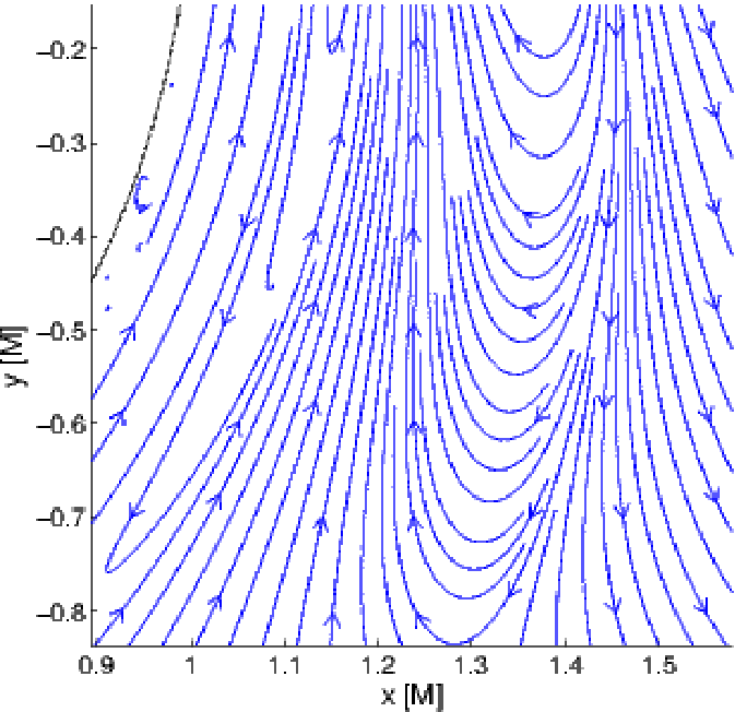
We further notice that in the equatorial plane the asymptotically perpendicular magnetic field (, ) will have zero longitudinal component regardless the field definition also in the vicinity of the black hole (only equatorially vanishing terms from (2.27) appear in the definition of in eq. 2.11). In other words the field lines reside in the equatorial plane in this special case. This might not be that visually apparent from the right panel of fig. 2.7. Therefore we add a series of equatorial sections in fig. 2.8 to reveal the field in the equatorial plane. Three equatorial observers, namely FFOFI, co-rotating KEP+FFO and counter-rotating KEP+FFO are involved in the comparison. We observe that free fall with (FFOFI) results in the aligned magnetic field lines in the Schwarzschild limit which we observed also in AMO components in fig. 2.7 as a result of taking its asymptotic form for . On the other hand, nonzero angular momentum of KEP+FFO observers which are freely falling with under causes twisting of the field lines even in the Schwarzschild case since the four-velocity and other tetrad vectors components do not take their asymptotic form with although the does. When the spin is employed the lines of force twist in a rather complex way regardless the choice of the observer. Complex layering of the field lines emerges in the narrow zone above the horizon. In order to stretch this tiny yet very interesting area and make it more convenient for visualisation we rescale the radial component introducing the dimension-less coordinate which squeezes the horizon into a single point and radial infinity into the circle . Rescaled coordinate is employed in bottom panels of fig. 2.8.
In the series of stereometric projections in fig. 2.9 we observe the interplay between the aligned and perpendicular magnetic field components using AMO definition of the field on the extreme Kerr background. We start with the aligned situation where the expulsion of the field is observed and gradually increase the perpendicular component to see that it generally causes intricate deformations of the field lines and allows them to penetrate the horizon even in the extreme Kerr case.
In fig. 2.8 we observe that the field twisting caused by the interplay between the black hole rotation and the horizontal component of the prescribed magnetic field is accompanied by intensive layering of the magnetic field in the narrow zone above the horizon. In fig. 2.10 we compare the detailed structure of the magnetic layer zone as measured by several distinct observers. We observe that magnetic layers are present regardless the choice of the frame although their actual shape changes as we switch between them. It is thus apparent that magnetic layers do not emerge as a observer effect. They rather originate directly from the interplay between the frame-dragging effect and prescribed magnetic field which is confirmed by observing layered magnetic structures also in observer independent AMO components.
Simulations of non-vacuum magnetospheres carried out in the framework of force-free electrodynamics (FFE) often reveal similar magnetic layers in which the direction of the field changes sharply. FFE assumes that plasma is streaming solely along the magnetic field lines and such layers thus become current sheets. See Spitkovsky (2006) for the simulation of pulsar magnetosphere in which the current sheets develop.
Electric field
Until now we have paid hardly any attention to the electric fields felt by the test charges in a given setup of Kerr black hole embedded in the asymptotically uniform magnetic field with general orientation with respect to the rotation axis. To correct this we present a summary of nonzero electric field components for various field definitions, observers and values of the spin parameter in tab. 2.1. We distinguish whether or components (or actually both) act as a source terms of a given electric field component. We treat separately the case of equatorial plane where part of the components diminish. Exploring tab. 2.1 we notice particularly that nonzero electric field is measured even in the Schwarzschild limit in the case of FFOFI and KEP observers.


Stereometric projections of AMO electric fields above extreme Kerr BH are presented in fig. 2.11 to illustrate the profound changes in the field line structure which accompany the onset of perpendicular magnetic field component which disrupts the symmetry of aligned case.
| field definition | ||||
|---|---|---|---|---|
| AMO | 0 | , , | ||
| , , | ||||
| , , | ||||
| , , | , | , , | ||
| ZAMO coord. | 0 | , , | ||
| , , | ||||
| , , | ||||
| , , | , | , , | ||
| ZAMO tetrad | 0 | , , | ||
| , , | ||||
| , , | ||||
| , , | , | , , | ||
| FFOFI coord. | 0 | , , | ||
| , , | , | |||
| , , | , | |||
| , , | , , | , , | ||
| FFOFI tetrad | 0 | , , | ||
| , , | , | |||
| , , | , | |||
| , , | , , | , , | ||
| KEP coord. | 0 | |||
| KEP tetrad | 0 | |||
In the series of plane sections in figs. 2.12 and 2.13 we compare the structures of the electric fields as measured by ZAMO and FFOFI observers. First we present the situation of aligned field () in which all poloidal sections of the fields coincide due to the symmetry (top panels of fig. 2.12). We notice that in the FFOFI tetrad (unlike the ZAMO tetrad) the electric field is expelled from the horizon of the extreme BH. Once the non-aligned field is considered (by setting ) the symmetry is lost and poloidal sections for different values of generally differ (see the bottom panels of fig. 2.12 and fig. 2.13). The effect of electric expulsion is gone once the non-aligned field is considered.
Stereometric projections in fig. 2.14 reveal that in the renormalized components the expulsion of the electric field out of the horizon of the extreme Kerr is present not only for the FFOFI test charge but also for the test charge with ZAMO four-velocity (while in the ZAMO tetrad the field lines are not expelled). Azimuthal component which is present in the FFOFI case causes winding of the field lines while the ZAMO field lines remain confined to a given poloidal sections. Bottom panels of fig. 2.14 illustrate that setting generally disrupts the symmetry and allows the field lines to penetrate the horizon regardless the spin value.
The expulsion of the electric field as observed in the FFOFI tetrad is further studied in fig. 2.15 where we provide series of poloidal plane sections for the aligned background field which differ in the spin value. Such discussion allows us to visually reveal the mechanism of the expulsion which takes place in the case of the extreme spin value. LIC patterns are also employed to help to reveal this effect.
Electric field is generally very sensitive to the value of spin parameter which is not that surprising since the field itself has gravitomagnetic origin by which we mean that it arises from the interplay between the background magnetic field and spin induced frame-dragging effect. As a consequence we measure no AMO electric field in the Schwarzschild limit since all vanish with . Naturally this does not necessarily mean that all observers will measure zero electric field. We have seen, for instance, that even in the case of zero spin the non-stationary FFOFI observer may observe nonzero electric field induced due to his radial velocity component . Nevertheless these electric components asymptotically diminish since the observer is asymptotically static.
The question of the expulsion of the electric field has been addressed in the case of aligned background field. Unlike the magnetic expulsion where the radial AMO component vanishes at the horizon for here the analogical component does not vanish. Thus the electric expulsion is merely an observer effect. We have seen that in the ZAMO tetrad the electric field was not expelled while in the FFOFI one it was. We recall that also the magnetic field is fully expelled in the FFOFI frame.


2.5.2 Electromagnetic field around drifting black hole
In this section we shall discuss the electromagnetic fields around Kerr black hole which is drifting in a general direction through the oblique uniform magnetic field. Components of EM tensor describing such field were derived in sec. 2.3 in terms of Lorentz transformation of former non-drifting solution given by eqs. 2.27, 2.28.
Resulting system provides highly simplified though not unrealistic model of conditions occurring in a diluted gaseous medium in the vicinity of the inner edge of the accretion disk. This region may be threaded by the external large-scale magnetic field which we model by oblique uniform field in our setup. Gravitomagnetic effect acts on the field enriching profoundly its structure as we have seen in previous section. Observer dependence of the EM field components has also been discussed previously. In addition to these effects we introduce the translational uniform motion of the black hole itself bringing extra parameters to the system. See Karas & Kopáček (2009) for a discussion of astrophysical relevance of our model.
Lorentz transformation of the field changes its asymptotical form – in general it changes the direction of the former magnetic field and induces electric field which was not present in the asymptotic region of non-drifting BH (for asymptotically static observers at least). In the previous section we observed that interaction between BH’s rotation and perpendicular component of the magnetic field causes complex twisting of the field lines and that a narrow zone of magnetic layers emerges above the horizon regardless the choice of the observer.
In fig. 2.16 we introduce the drift in the case of extreme BH embedded in the aligned field in order to detect the drift impact upon the field most clearly. We observe that the Meissner effect is suppressed by the drift. We note that with the drift velocity increasing the shock front develops in which the field has complex layered structure which gradually enhances as the velocity rises. Besides the magnetic layers we newly observe the pair of magnetic null points which emerge for the sufficiently rapid drift. Sites of zero magnetic intensity leave the charged particles prone to the acceleration by the electric field which is generally not vanishing here. The layered field structures which surround the neutral point present the sites of possible magnetic reconnection (Karas & Kopáček, 2009, and references therein). Magnetic layers and neutral points are further explored in fig. 2.17 using LIC patterns with the strength of the field being encoded by the color scale.
From fig. 2.10 we recall that magnetic layers emerge also in the non-drifting case as a consequence of a perpendicular component of the field. Layering accompanied with the drift through the aligned field thus may be attributed to the tilt arising from the Lorentz transformation. The neutral points, however, only appear in the drifting case.
In stereometric projections fig. 2.18 we compare magnetic field measured in the FFOFI frame to that captured by the ZAMO renormalized components. In both the cases the aligned non-drifting field above the extremal BH is fully expelled, the only difference being that the FFOFI field is slightly azimuthally twisted (see fig. 2.6). When the drift is introduced, however, the behaviour of the field lines differs strikingly as they are dragged in the opposite direction. FFOFI lines stretch in the drift direction in an intuitive way while in the ZAMO renormalized components they are dragged backwards manifesting profound differences between the two field definitions.
Electric field also reacts markedly when the drift is introduced. In fig. 2.19 we explore its impact upon the FFOFI electric components above the horizon of the extremal BH in the poloidal plane section. Gradually increasing the drift velocity we observe how the topology of the field evolves. We note that without the drift the electric field asymptotically decays whereas the drift induces non-vanishing electric field which overruns the original one. Thus the global impact of the drift is more dramatic compared to what we observed in the case of magnetic field. Besides overall changes of the field we also notice progressive layering in the narrow region above the horizon. Similarly to their magnetic analogue, the electric layers are also present regardless of the choice of the observer and their origin may be attributed to the tilting of the originally aligned magnetic field due to the drift.
We also explore the electric field in the equatorial plane in fig. 2.20. Since we start out from the aligned magnetic field and the drift is restricted to be perpendicular to the axis () the field lines will reside in the plane (see tab. 2.1). The rescaled radial coordinate is employed. We compare the tetrad components of ZAMO, FFOFI and both co-rotating and counter-rotating KEP+FFO. The drift changes the structure of the field completely including the asymptotic region. Although the fields differ from each other noticeably for different frames, in all the cases the neutral points are formed (at different location, though) once the sufficiently rapid drift is introduced.
We conclude that the translational motion of the black hole through the uniform magnetic field enriches profoundly the structure of the resulting electric and magnetic fields. We observed that in the case of axisymmetric background the drift causes a formation of a narrow zone in which the fields (both electric and magnetic) are heavily layered and the layering progressively enhances with the rising drift velocity. However, we observe such effect also for nondrifting oblique fields (see fig. 2.10) and therefore we attribute the formation of the layers to the perpendicular component which arises from the field’s tilt in the case of drift through the aligned magnetic field. Nevertheless only in the drifting scenario we can observe such topology of layers which leads to the formation of neutral points. These were observed for both, magnetic as well as electric fields.


2.6 Motion of charged test particles
Off-equatorial, energetically bound motion of charged particles in strong gravitational and electromagnetic fields is pertinent to the description of accretion disk coronae around black holes and compact stars. In recent papers (Kovář et al., 2008; Kovář et al., 2010) we discussed the existence of energetically-bound stable orbits of charged particles occurring outside the equatorial plane, extending thus a large variety of complementary studies (e.g., Bičák et al., 1989; Stuchlík et al., 1999; Prasanna, 1980; Prasanna & Sengupta, 1994; Aliev & Özdemir, 2002, and further references cited therein). Particles on off-equatorial stable trajectories form a coronal flow that is possible at certain radii and for certain combinations of the model parameters, namely, the specific charge of the particles, the conserved energy and the angular momentum of the particle motion, the strength and orientation of the magnetic field, and the spin of the central body.
We assume that the magnetic field permeating the corona has a large-scale (ordered) component (Bisnovatyi-Kogan & Lovelace, 2007). In this case, charged particles can be trapped in toroidal regions, extending symmetrically above and below the equatorial plane and forming two halo lobes. However, this trapping happens only for certain combinations of model parameters (Kovář et al., 2010).
We consider two types of the model setup: a rotating (Kerr) black hole in an asymptotically uniform magnetic field parallel to the symmetry axis (Wald, 1974; Tomimatsu & Takahashi, 2001; Koide, 2004; Koide et al., 2006), and a non-rotating star (described by the Schwarzschild metric) endowed with a rotating magnetic dipole field (Petterson, 1975; Sengupta, 1995). Both cases can be regarded as integrable systems with the electromagnetic field acting as a perturbation.


The above-mentioned lobes are defined by the figures of the effective potential in the poloidal plane. These were previously studied in the context of charge separation that is expected to occur in pulsar magnetospheres (Neukirch, 1993, e.g.). Here, we address whether the trajectories within these lobes are regular (i.e., whether the system is integrable), or if they instead exhibit a chaotic behavior. A related problem was studied recently by Takahashi & Koyama (2009) in an attempt to find a connection between chaoticness of the motion and the spin of a rotating black hole residing in the center. These authors suggest that chaotic behavior occurs for certain values of the black hole spin, while for others the system is indeed regular.
The idea of investigating the connection between the spin of a black hole and chaoticness of motion of matter near its horizon is very interesting for the following reason. Because of high degree of symmetry of the background spacetime, the unperturbed motion is regular (Carter, 1968); no chaos is present. The electromagnetic perturbation may trigger the chaos, however, its effect can be expected to diminish very near the horizon, where strong gravity of the black hole should prevail. This is also the region where the spin effects are most prominent. Further out various other influences become important due to distant matter and the turbulence in accreted material. Therefore the connection between the spin and the motion chaoticness is best applicable in the immediate vicinity of the black hole, i.e. within the inner parts of corona.
The recurrence analysis (Marwan et al., 2007) provides us with a powerful tool for the investigation of complex dynamical systems. The method examines the recurrences of the system to the vicinity of previously reached phase space points. It has been typically adopted to study the experimental data, where often only some (if not just one) of the phase space variables are known from the measurements. Takens’ embedding theorems (Takens, 1981) are then used to reconstruct the phase space portrait of such a system. In our study we are equipped with the full phase space trajectory from the numerical integration of the equations of motion, so that we can use the recurrence analysis directly.
It appears that the method of Recurrence Plots has not been employed in the context of relativistic astrophysical systems yet. To this end, one needs a consistent definition of the neighborhood of a point in the phase space in a curved spacetime. Below, we discuss the phase space distance and suggest a form of the distance norm suitable in such circumstances.

2.7 Equations of motion and the effective potential
The phase space trajectories of integrable systems are regular, meaning that they are bound to the surface of an -dimensional torus, where is the number of degrees of freedom. The torus is determined uniquely by constants of motion that are present in such a system. Its behavior can be explored by Poincaré surfaces of section, which are defined by intersections of the phase space trajectory with a -dimensional plane (Lichtenberg & Lieberman, 1992). On the other hand, non-integrable chaotic systems generally have fewer integrals than the number of degrees of freedom. In general, both the regular and the chaotic orbits may coexist in the phase space of a single system.
Chaotic orbits are ergodic on the given hypersurface. Its dimension is now larger than , and the section points thus fill areas in the plot of the Poincaré surface. However, depending on the initial conditions, regular orbits can also appear in non-integrable systems. Such orbits maintain the value of some additional constant of motion, although it is not generally possible to write this constant in an explicit form. In the context of motion around black holes perturbed by (weak) external sources, various aspects of chaos were studied e.g. by Karas & Vokrouhlický (1992); Nakamura & Ishizuka (1993); Podolský & Veselý (1998), and very recently by Semerák & Suková (2010).
A standard approach to an integrable system with a non-integrable perturbation assumes complete control over the strength of the perturbation (i.e., the perturbation can be set to be arbitrarily weak). If this were the case, we could first switch the perturbation completely off, analyze the orbits, and then observe the impact of gradually increasing the perturbation strength upon these orbits. However, the class of off-equatorial bound orbits only exists when the electromagnetic term is strong enough to balance the gravitational attraction of the central body. Then the (sufficiently strong) perturbation is by itself the cause of the new kind of the regular motion that happens outside the equatorial plane.


Having this delicacy on mind, we shall use the usual Hamiltonian formalism to express equations of motion governing the trajectories. We first construct the super-Hamiltonian (Misner et al., 1973),
| (2.69) |
where and are the rest mass and charge of the test particle, is the generalized (canonical) momentum, is the metric tensor, and denotes the vector potential of the electromagnetic field. The latter is related to the electromagnetic tensor by . Unless otherwise stated, we will use geometrical units, (see Appendix A).
The Hamiltonian equations are given as
| (2.70) |
where is the affine parameter, denotes the proper time, and is the standard kinematical four-momentum for which the first equation reads .


In the case of stationary and axially-symmetric systems, we identify two constants of motion, namely, the energy and angular momentum . From the second Hamiltonian equation (2.70) we obtain
| (2.71) | |||||
| (2.72) |
The trajectory is specified by the integrals of motion , , and the initial values , and . The initial can be calculated from the normalization condition, (we always choose the non-negative root).
The effective potential can be derived in the following form:
| (2.73) |
where
| (2.74) | |||||
| (2.75) | |||||
| (2.76) |
and where we introduce specific quantities , and the specific charge . Local minima of reflect the location of stable orbits of test particles. Off-equatorial potential minima were identified and various types of potential lobes were discussed elsewhere (Kovář et al., 2010, see)11 1 We have employed the method of effective potential to study the stability of the motion, however, we note that the force formalism (Abramowicz et al., 1995; Kovář & Stuchlík, 2007) can serve as a very efficient alternative tool. In particular, the off-equatorial motion of charged particles can be examined via the procedure described in Kovář et al. (2010). This allows us to localize minima of the effective potential around which the stable orbits occur.. We can express the effective potential (2.73) also as a function of and , and use it to determine the boundaries of allowed regions in Poincaré surfaces of section for a given value of .


We employ the Kerr metric in standard Boyer-Lindquist coordinates , , , given by eq. (2.1). It is sufficient to consider positive values of the spin parameter without loss of generality (the cases of prograde and retrograde motion are distinguished by the sign of the particle charge and the orientation of the magnetic field). By setting the metric (2.1) reduces to the static one describing the Schwarzschild spacetime.


At this point, a note is worth on the adopted computational scheme which we have employed to study the trajectories and to detect the chaotical behavior. In order to reach reliable results, we coded several approaches and we checked their stability and precision. We employ the multi-step Adams-Bashforth-Moulton solver to determine the phase-space trajectory by numerical integration of eqs. (2.70). In some cases, when a higher precision is demanded, we use the -th order Dormand-Prince method that belongs to the family of explicit Runge-Kutta solvers with adaptive stepsize. This method improves the accuracy significantly, as can be verified by checking the conservation of the integrals of motion along the trajectory. However, the improved accuracy comes at the expense of computational time, as the adopted Dormand-Prince scheme is more computationally demanding than the Adams-Bashforth-Moulton solver.


Furthermore, it is well-know that, when dealing with Hamiltonian systems, the most appropriate solvers are those which respect the symplectic nature of Hamiltonian dynamics (Yoshida, 1993, e.g.). We therefore employed also the implicit Gauss-Legendre Runge-Kutta (GLRK) method, which is a symplectic scheme. Indeed, we confirm that this code provides the most reliable results, especially in the case of long-term integration. The difference in the accuracy between GLRK and non-symplectic solvers reaches several orders of magnitude and it is generally more apparent in the case of chaotic trajectories, as expected. However, the cost in terms of the computational time is also non-negligible, and so we only use the GLRK method to achieve very accurate long-time determination of the trajectory in several exemplary runs. Detailed comparison of the integrators is presented in Appendix B.
2.8 Recurrence analysis
The Kerr metric is well-known and the analysis of test particle motion in this spacetime was carried out in many papers (Misner et al., 1973). Among important features of the Kerr metric is the fact that the particle trajectories are integrable, and so the chaos can set in only when perturbations of the background gravitational field are introduced or additional electromagnetic interaction with fields of external sources are allowed. This is also where recurrence analysis can be helpful.

Methods of phase space recurrences have been successfully applied to a wide range of various empirical data, not only in physics but also related to physiology, geology, finances and other fields. Recurrence plots are especially suitable for the investigation of rather short and nonstationary data. On the other hand, the method of recurrence analysis has not yet been widely applied to study the dynamical properties of motion in relativistic systems. We thus briefly summarize this approach for our context.
Besides more traditional methods of the numerical analysis of dynamical systems, such as a visual survey of Poincaré surfaces of section or the evaluation of the Lyapunov spectra (Skokos, 2010), the recurrence analysis is a rather novel technique, based on the analysis of recurrences of the system into the vicinity of its previous states.
Recurrence Plots (RP) are introduced as a tool of visualizing the recurrences of a trajectory in the phase space (Eckmann et al., 1987). The method is based on examination of the binary values that are constructed from the trajectory . Results of the orbit analysis can be quantified statistically in terms of the Recurrence Quantification Analysis (RQA).22 2 We use the CRP ToolBox (Marwan et al., 2007, p. 321) in Matlab (R2009b) to construct RPs and to evaluate RQA measures.
The RP construction is straightforward regardless of the dimension of the phase space. We only need to evaluate the binary values of the recurrence matrix , which can be formally expressed as follows:
| (2.77) |
where is a pre-defined threshold parameter, the Heaviside step function, and specifies the sampling frequency. The sampling frequency is applied to the time segment of the trajectory under examination. There is, however, no unique prescription for the appropriate definition of the phase space norm in eq. (2.77). We can consider a purely abstract vector space and apply one of the elementary norms , (Euclidean norm) or (maximum norm). Some aspects of the appropriate choice of the norm are deferred to sec. 2.8.1.

Finally, we need to specify the value of the threshold parameter . To this end we follow the suggestion of Marwan et al. (2007, sec. 3.2.2) and relate to the standard mean deviation, , of the given data set. Setting is advantageous because the proportionality constant , once adjusted to obtain a properly filled Recurrence Plot, remains valid (with only minor adjustments) for all data sets of other trajectories. We therefore normalize the time series of each coordinate separately to zero mean and .
The binary valued matrix represents the RP which we get by assigning a black dot where and leaving a white dot where . Both axes represent a time segments over which the data set (the phase space vector) is being examined. RP is thus symmetric; the main diagonal is always occupied by the line of identity (LOI).
Recurrence Plots contain wealth of information about the dynamics of the system (Thiel et al., 2004a). Different pieces of knowledge are encoded in large-scale and short-scale patterns (Marwan et al., 2007, sec. 3.2.3). To decide if a particular trajectory is a regular or a chaotic one, the determining factor is the presence of diagonal structures in the RP. Diagonal lines in the RP reflect the time segments of phase space trajectory during which the system evolution proceeds in a regular way. It captures the epoch when the trajectory proceeds almost parallel to its previous segment, i.e. within the -tube around that segment. Hence, integrable systems exhibit themselves by diagonally oriented structures in their RP. On the other hand, if the motion is chaotic the diagonal lines disappear and the diagonal features become shorter, as the trajectories tend to diverge quickly. As a result, more complicated structures appear in the RP.

We stress that the interpretation of the RP is primarily intuitive. We refer to the review paper Marwan et al. (2007, sec. 3.2.3) where the patterns appearing in the RP and their relation to the current dynamic regime are analyzed in detail. Although basic conclusions may be inferred in general (e.g. distinction between regular versus chaotic regime) the fine structure of the RP depends heavily on the properties of a given dynamic system. In order to gain more insight into the way in which various dynamical regimes manifest themselves in our system we typically present RPs accompanied by corresponding Poincaré surface of section throughout this text.


Visual behavior of RP and its complexity is quantitatively reflected in RQA. The RQA evaluates statistical characteristics of the recurrence matrix . First of all, we define the recurrence rate () as a density of points in RP,
| (2.78) |
Now we can turn our attention to diagonal segments in RP. Their length draws distinction between regularity and chaos. The histogram records the number of diagonal lines of length . It is formally given as follows:
| (2.79) |
This histogram defines the determinism factor (), defined as a fraction of recurrence points, which form the diagonal lines of length at least to all recurrence points,
| (2.80) |

The average length of diagonal lines (where only lines of length at least count) is
| (2.81) |
and the corresponding divergence () is defined as inverse of the length of the longest diagonal line ,
| (2.82) |
is in its very nature closely related to the divergent features of the phase space trajectory, and so it was originally (Eckmann et al., 1987) claimed to be directly related to the largest positive Lyapunov characteristic exponent . On the other hand, theoretical considerations justify the use of as an estimator only for the lower limit of the sum of the positive Lyapunov exponents (Marwan et al., 2007, sec. 3.6). Nevertheless, a strong correlation between and arises in numerical experiments (Trulla et al., 1996).
The quantification measure is defined as the Shannon entropy of the probability of finding a diagonal line of length in the Recurrence Plot,
| (2.83) |
where is a total number of diagonal lines: .
Analogous statistics may be performed for vertical as well as the horizontal segments (RP is symmetric with respect to the main diagonal). These segments are generally connected with periods in which the system evolves during its laminar state. To this end, the histogram records the number of vertical lines of length and it can be constructed as follows:
| (2.84) |
In analogy with the diagonal statistics histogram, is used to define the vertical RQA measures. Laminarity () is defined as a fraction of recurrence points that form vertical lines of length at least to all recurrence points,
| (2.85) |
The trapping time () is an average length of vertical lines,
| (2.86) |
Finally, the length of the longest vertical line () can also be of some interest.
RQA measures the crucial dependence of RP on the value of the threshold parameter, , which must be adjusted appropriately to a given data set. This lack of invariance is a drawback of both RPs and RQA. Nevertheless, it was shown (Thiel et al., 2004b) that stable estimates of various dynamical invariants, such as the second order Rényi entropy and the correlation dimension, can be inferred if is kept within a reasonable range. Since we shall use the standard RQA measures to compare the dynamics between test particles with different initial conditions, we have to eliminate the numerical effect of variances in the range of coordinate values spanned by these trajectories. We achieve this by fixing the value of .

After the brief set of preliminaries we are now prepared to proceed to the intended application of the recurrence analysis in the next section.
2.8.1 Phase space recurrence in the curved spacetimes
When analyzing the dynamics in the general relativistic context the fundamental question arises whether the distinction between chaotic and regular motion is coordinate dependent or not. To this end Motter (2003) infers the transformation law for Lyapunov exponents. He concludes that although the Lyapunov exponents themselves are not invariant they transform in such a way that positive Lyapunov exponents remain positive and vice versa. In other words the distinction between regular and chaotic dynamics may be drawn invariantly.
In order to give the notion of recurrence a rigorous and, at the same time, an intuitive sense, we can employ the formalism (Thorne & MacDonald, 1982) that is based on an appropriate selection of a family of spacetime-filling three-dimensional spacelike hypersurfaces (foliation) of constant time . The timelike curves orthogonal (in a spacetime sense) to the hypersurfaces may be regarded as the world-lines of a family of fiducial observers (FIDO) who naturally parameterize their world line by proper time (whose rate of change generally differs from that of ). FIDO identify each spatial hypersurface along his world line as a slice of simultaneity. The geometry of this spacetime slice is given by 3-metric :
| (2.87) |
where stands for the spatial part of FIDO’s four-velocity and for the spatial part of the spacetime metric. Considering also the time coordinate, can be regarded as a projector onto the three-dimensional spatial hypersurface.
Our selection of FIDOs will be restricted here to those moving along the Killing direction (thus seeing an unchanging spacetime geometry in their neigbourhood). We shall also demand that all the hypersurfaces of simultaneity which they constitute have an identical spatial geometry. Finally, we require that FIDO’s proper time becomes asymptotically identical to the coordinate time . In the case of Kerr spacetime (as an example of stationary and axisymmetric spacetime) these restrictions lead to the identification of the FIDOs with the zero angular momentum observers (ZAMOs), see Thorne & MacDonald (1982). Orthonormal tetrad of ZAMO is given by eqs. (2.44)–(2.47).

Projecting an arbitrary four-vector onto ZAMO’s hypersurface of simultaneity directly results in the following 3-dimensional quantities,
| (2.88) | |||||
| (2.89) |
here, ( for ZAMO) and, consequently, .
ZAMO tetrad components are given as
| (2.90) | |||||
| (2.91) |
The hypersurface components of the phase space constituents and , as measured by ZAMO, are then:
| (2.92) | |||||
| (2.93) |
The spatial 3-metric is
| (2.94) |
where represents the spatial distance from the origin of the tetrad, i.e. ZAMO’s current location. ZAMO is not an inertial observer, which generally causes the first order corrections to the Minkowskian metric . But these do not enter the spatial part of the metric. Thus the 3-metric within the spatial hypersurface is a Euclidean one, with the deviations of second order in the distance from the spatial origin on ZAMO’s world-line.


We will use ZAMO’s metric at distances up to the value of the threshold parameter . The Euclidean metric according to eq. (2.94) will be therefore justified if , where stands for a constant (for a given ZAMO). has the dimension of length and characterizes the curvature of the hypersurface. We suggest setting , where represents the Kretschmann scalar evaluated from the Riemann curvature tensor. In the case of the Kerr black hole the Kretschmann scalar may be expressed in a surprisingly simple form (Henry, 2000). While constructing the Recurrence Plots, we check whether the condition remains satisfied.
The above-mentioned adoption of preferred observers is needed in order to maintain an operational criterion of chaos and be able to formulate an explicit form of the equations for RQA measures in a curved spacetime. Here the notion of the phase space distance plays a role. In Kerr metric (or another axially symmetric stationary spacetime), Fiducial Observers (a.k.a. FIDOs) represent a natural selection of preferred observers. Obviously, this option is not unique, and so a detailed appearance of the recurrence plots is also ambiguous to certain extent. But not so the main conclusions that we infer regarding the chaoticness versus regularity of the system behavior, because this distinction can be eventually traced down to the exponential versus polynomial growth of the separation with the particle proper time along neighboring trajectories.
We can deduce the kind of transformation between different families of observers that could affect our conclusions: these are transformations involving exponential dependencies on observer’s phase-space position. For example transformation to accelerated frames and spacetime points in the vicinity of singularities may need a special consideration, as well as the investigation of highly dynamical spacetimes that are lacking symmetries. On the other hand, selecting LNRF to define ZAMOs in (weakly perturbed) Kerr metric outside the black hole horizon appears to be a well-substantiated choice.

Similar arguments for the adoption of preferred observers on the basis of spacetime symmetries have been elaborated in greater detail by Karas & Vokrouhlický (1992) in the context of Ernst’s magnetized black hole, which is another particularly simple (static) exact solution of Einstein-Maxwell equations exhibiting the onset of chaos as the magnetic field strength is increased.
2.9 Kerr black hole in uniform magnetic field
Large-scale magnetic fields are known to be present in cosmic conditions. They can exist around black holes, which do not support their own magnetic field but may be embedded in fields of distant sources. In the case of neutron stars, dipole-type magnetic fields of very high strength often arise. We concentrate on black holes in this section and defer the case of a magnetic star to sec. 2.10.

By employing the uniform test field solution (Wald, 1974) we incorporate a weak large-scale magnetic field near a rotating black hole. The vector potential can be expressed in terms of Kerr metric coefficients (2.1) as follows,
| (2.95) | |||||
| (2.96) |
where is magnetic intensity and stands for the test charge on the background of Kerr metric. The terms containing can be identified with the components of the vector potential of Kerr-Newman solution (although the test charge does not enter the metric itself). An example of an integrated trajectory is shown in fig. 2.21. Wald (1974) has shown that the black hole selectively accretes charges from its vicinity, until it becomes itself charged to the equilibrium value
| (2.97) |
We remark that the particle charge appears always as a product with or in the formula (2.73) for the effective potential, as well as in equations of motion (2.70). Therefore, the simultaneous alteration of , and values, preserving the products and , does not affect the particle dynamics. If we further assume that is maintained, we only need to specify the value of to uniquely determine a particular trajectory. However, since we do not restrict ourselves to the case we decide to always explicitly specify the values of and .
2.9.1 Motion within the potential lobes
Our previous analysis (Kovář et al., 2010) concludes that the off-equatorial bound orbits are allowed only for test particles obeying simultaneously the two conditions, and . Four distinct types were found (see fig. 2.22) and we examined the dynamics of test particles in all of these types. The results for different types are comparable, and so we present here only the analysis of two of them, namely the types Ia and Id. While raising the energy level from the local minima of the symmetric halo orbits, we observe that the off-equatorial lobes grow and eventually merge with each other once the energy of the saddle point in the equatorial plane is reached. If we further increase the energy the behaviour between the two classes differs profoundly. For Ia we observe that the lobe eventually opens toward the horizon allowing the particle to fall onto the black hole. On the other hand in the Id setup the merged lobe breaks “toward infinity” allowing the particle to escape in the axial direction when the energy is raised sufficiently.
The size of the lobes is controlled by the specific energy . Employing the Poincaré surfaces of section and the Recurrence Plots we investigate how the regime of the particle motion changes with . This parameter appears as a suitable control parameter producing a sequence of bound trajectories while all other parameters (and the initial position) remain fixed. For the sake of comparison we first present the case of a fully integrable system of a charged test particle on the pure Kerr-Newman spacetime (fig. 2.23). The motion occurs in the potential lobe around the local minimum in the equatorial plane; there are no halo orbits above the horizon in this case (Kovář et al., 2010; de Felice, 1979).
On the Kerr background with Wald test field we first analyze the sequence of trajectories of Ia type. Figure 2.24 shows regular motion occurring in the off-equatorial lobe. Increasing the energy level (while keeping all other parameters fixed) above the value in the equatorial saddle point results in a transitional regime depicted in fig. 2.25. The onset of chaotic features does not occur as a direct consequence of the lobe merging. We rather observe that the orbit bound in merged (cross-equatorial) lobe remains regular until the particle notices the possibility of crossing the equatorial plane which happens when its energy is increased sufficiently. Once the motion becomes cross-equatorial, chaotic features appear. By increasing the energy even more we approach the critical value when the lobe opens and allows the particles to fall onto the horizon. For energies slightly below this limit we detect a fully chaotic regime of motion (fig. 2.26).
Similar sequence of trajectories is analyzed in the case of Id class of the topology of the potential wells. Three typical trajectories found in this case are shown: regular off-equatorial, regular cross-equatorial and chaotic cross-equatorial orbit. First we present their overview in fig. 2.27 which shows the main difference from the Ia series clearly: the presence of fully regular cross-equtorial orbits. In fig. 2.28 we compare Poincaré surfaces of section and Recurrence Plots of these trajectories. Unlike previous series we distinguish from in the Poincaré surface of section.
Figure 2.29 shows an alternative representation of the recurrence plots, where the phase space distance separating the given pair of points of the trajectory is encoded by different colors. Again, by comparing the two panels one can clearly recognize how the diagonal structures disintegrate into scattered points as the chaos sets in.
From the survey of the first series of Poincaré surfaces of section and the Recurrence Plots (figs. 2.24–2.26) we may only conclude that the transition from the regular to chaotic regime occurs somewhere close to the value . In order to localize this transition more precisely we evaluate RQA measures for 400 trajectories with the energy spread equidistantly over the interval . In figs. (2.30) and (2.31), we observe a sudden change of the behavior of the statistical measures at , reflecting a dramatic change of the particle dynamics.
Moreover, we know that the divergence is related to the Lyapunov exponents, and in fig. 2.30 we observe that it suddenly rises at , meaning that the trajectories become more divergent when this energy is reached. All of these indications combined lead to the conclusion that this energy level represents a critical value at which a transition from regular to chaotic regime occurs.
Similarly we perform the RQA for the sequence of orbits of Id type which we analyzed qualitatively in fig. 2.28. Visual survey suggests that the suspicious interval in which the transition from regular to chaotic dynamics shall occur is . We calculate 200 trajectories with energies equidistantly spread over the given range while other parameters of the system are fixed at values used in fig. 2.28. In figs. 2.32 and 2.33 we observe that all queried RQA measures exhibit sudden change in its behaviour at . This is where the dynamic transition between the regimes occurs. Transition from the regular motion to the chaos is detected not only by diagonal RQA measures but also by the vertical ones.
We conclude that the energy of the particle acts as a governing factor determining the dynamic regime of motion. Our survey across various initial conditions has shown that motion in potential wells of the type Ia in a Wald test field is generally regular. Chaos appears well after the merging point of the lobes and close to the critical breaking energy. We have verified that all queried RQA measures, i.e. not only those based on diagonal lines in RP, react to the transition from the regular to chaotic regime of motion, allowing us to localize precisely the transition. This was fully confirmed also in the other two types (classes Ib and Ic of our typology in fig. 2.22).
2.9.2 The effect of spin on the chaoticness of motion
Much attention has been recently focused towards the problem of determining the black hole spin from the properties of motion of surrounding matter (Narayan, 2005; Reynolds & Nowak, 2003). The astrophysical motivation to address these issues arises from the fact that cosmic black holes are fully described by three parameters – mass, electric charge and spin. While the methods of mass determination have been widely discussed (Casares, 2007; Vestergaard, 2010; Czerny & Nikolajuk, 2010, e.g.), the electric charge is considered to be negligible because of rapid neutralization of black holes via selective accretion. However, determining the spin is a much more challenging task: the spin is important, but its influence is apparent only very near the black hole horizon (Murphy et al., 2009).
 |
 |
One can raise a question of whether the value of spin parameter of the Kerr black hole affects the dynamical regime of motion in the immediate neighborhood of the black hole. In other words, we ask if the spin parameter triggers or diminishes the chaoticness of the system. Answering this question is not straightforward because by altering the spin across an interval of values () we inevitably have to change some other variables of the system; otherwise the different cases could not be directly compared. Moreover, the location and the very existence of the potential lobes is not automatically ensured over the whole range of spin because of strong dependence.
We found that in order to keep the off-equatorial lobe at the initial position and the original size we need to increase the energy , roughly proportionally to the increment of . The effect of increasing exhibits itself by lifting the hyperplane of effective potential. To compensate for this effect we have to elevate the -plane at which we cut the potential, so that we obtain (roughly) the original closed contour (the potential lobe) inside of which the motion is confined. It turns out that this can be achieved by linking both quantities linearly.
First we compare the dynamics in the off-equatorial lobe in the range (for the topology of the effective potential changes) to which we linearly relate the energy range (whilst other parameters are kept fixed as follows: , , , , , ). By inspecting the Poincaré surfaces of section and performing the recurrence analysis for a large number of trajectories across the given range of and (exemplary cases presented in fig. 2.34) we come to the conclusion that there is no overall trend that could suggest that is the unique driving agent affecting the regime of motion. All trajectories in our survey exhibit a regular behavior, which is also in agreement with the previous conclusion that the motion in off-equatorial potential lobes associated with the Wald test field is generally regular.


We also examined the dynamics of test particles launched from the equatorial plane whose trajectories occupy the potential lobe extending symmetrically above and below the equatorial plane. A given lobe maintains its size for spin values and the related interval of energy . A survey across the given range of spin (energy) values reveals for this class of trajectories both chaotic and regular regimes. In fig. 2.35 we observe that for the lowest inspected spin, (), the regular motion dominates, although islands of chaotic behavior are also present. Increasing the spin (energy) we observe that regular trajectories gradually diminish. For () some regular orbits still appear, but they are already dominated by chaotic trajectories. For higher spins the traces of regular motion further diminish. We present the extreme case () in fig. 2.35 to illustrate this apparent chaotic takeover.
We conclude that for the class of orbits originating in the equatorial plane, spin could possibly act as a destabilization factor which triggers the chaotic motion if enhanced sufficiently. However since the energy is increased simultaneously it is not possible to attribute the observed dependence to the spin itself. On the other hand we have already seen in the above-given discussion (sec. 2.9.1) that energy may itself act as a key factor determining the dynamic regime of motion. Thus we suggest to attribute the observed triggering of the chaos to the increase of energy rather then spin .
We remark that a similar problem concerning the spin dependence of the motion chaoticness was addressed recently by Takahashi & Koyama (2009). Authors of the quoted paper employ a dipole magnetic test field upon a Kerr background and perform a study of test particle trajectories, concluding that increasing the value of the spin parameter stabilizes the motion in a given setup. Unlike our case, the topology of the effective potential in their scenario allows the chosen potential lobe to be maintained at a given location and roughly the same size (but not the same depth) even if varies while is kept constant. However increasing the spin allows the authors to set gradually lower and lower energies, for which more regular trajectories are found. This is not at all surprising in perspective of our results, where the energy proved to play a key role in determining the stability of motion. Although a direct comparison of presented surfaces of section differing only in value may suggest the spin dependence, there is no clear and unambiguous correlation. We thus suggest attributing the observed dependence primarily to the level of energy, which acted as a motion destabilizer also in our setup. In fact, even if a real trend with the spin is present, it is hard to disentangle it from a simultaneous change of .
The question of the dependence of the dynamics upon the other parameters of the system (, , ) was also addressed during the analysis. It appeared that above mentioned difficulties accompanying the analysis of the spin dependence became even more serious in this case. Namely, neither it was possible to maintain the given potential lobe for a reasonable range of values of selected parameter nor we were able to fix this problem by binding this parameter in some simple manner to some other parameter (e.g. energy ). In other words, none of these parameters itself may be regarded as a trigger for chaos.
2.9.3 Motion in potential valleys
Besides off-equatorial lobes, the potential may form another remarkable structure – an endless potential valley of almost constant depth which runs parallely to the symmetry axis (fig. 2.36). The poloidal orientation and asymptotical form of the valley are due to the fact that the Wald test field does not vanish at spatial infinity and it approaches the uniform magnetic field parallel to the symmetry axis.
The existence of such a potential corridor suggests that test particles with a particular range of parameter values could escape from the equatorial plane to large distance. We observe that a test particle in the potential valley can keep oscillating around the equatorial plane or it may escape from this plane completely, depending on its initial position in the phase space (see the upper left panel of fig. 2.37). We can examine the motion in the asymptotic region by rescaling the radial coordinate (upper middle panel of fig. 2.37). To achieve this, we use , where is the position of the outer horizon of the black hole.
The normalization condition allows one to express as a function of other phase space variables and parameters of the system. Intuition suggests that, considering particles launched from the equatorial plane (), the initial value is a governing parameter which decides whether the particle remains oscillating around or leaves it once forever. We can draw the isolines of selected values in the (, )-plane which we use as a surface of section () for the inspection of the test particle dynamics. Comparing acquired isolines for various values of with the empirically stated escape corridor of fig. 2.38 leads to the conclusion that they never coincide perfectly, although the correlation is quite high. In other words there is no definite threshold value of which would determine whether a selected combination of , (while other parameters are fixed) lets the particle launched at equatorial plane leave or oscillate around the plane.
In fig. 2.38 we observe several qualitatively different types of possible particle dynamics. Next to the effective potential contour we find closed and well-defined curves which represent the regular motion. Going further inside we notice that fragmented curves are present. Below them we find progressively more and more blurred patterns, which again signifies the onset of chaos. The inner parts of the potential lobe are occupied by the “escape corridor” where the particles can stream freely from the equatorial plane, as seen in fig. 2.37.
The trajectories represented by the closed curves in the surface of section differ profoundly from the disconnected curve orbits. The difference can be seen also in the direct projection onto the poloidal plane (upper right panel of fig. 2.37). While the trajectories of the first type gradually fill each particular compact region of given section, the latter forms bundles which curl through the projection plane resembling ribbons that bound regions which are never reached by the particle.

By employing the Recurrence Plots (bottom panels of fig. 2.37) we confirm that the dynamics differs significantly in these distinct modes of motion. Not surprisingly we obtain a typical regular pattern in the case of trajectory which forms a closed sharp curve in the surface of section (bottom left panel of fig. 2.37). A “ribbon–like” trajectory (fragmented curve in fig. 2.38) results in an ordered checkerboard pattern (bottom middle panel), which is known to be typical for periodic and quasi–periodic systems (Marwan et al., 2007). Finally, in the bottom right panel of fig. 2.37 we observe that a blurred curve trajectory exhibits slight chaotic behavior in its RP. The diagonal structures are partially disrupted and we notice that diagonal lines become bent as they approach the line of identity.
The class of escaping trajectories in the Kerr background was recently discussed by Preti (2010). The author suggests that a Wald electromagnetic field employed in this setup could serve as a charge separation mechanism for astrophysical black holes since the sign of the particle charge may determine whether a given particle escapes from the equatorial plane or becomes trapped in cross-equatorial confinement (or falls into the horizon).
2.9.4 Rotation number and fragmented tori
In the integrable system the trajectories in the phase space reside on the surface of the tori characterized by the values of integrals of motion which determine the characteristic frequencies of the orbit. Fundamental frequencies in our axisymmetric system are those of radial and latitudinal motion ( is cyclic coordinate). Once the system is slightly perturbed (by the magnetic field in our model) the tori characterized by the irrational ratio of frequencies survive which is assured by the Kolmogorov-Arnold-Moser (KAM) theorem. On the other hand the Poincaré–Birkhoff theorem tells us that the resonant tori with the rational frequency ratio will disintegrate into the chain of islands when we perturb the system (Lichtenberg & Lieberman, 1992). Trajectories belonging to the given chain are characterized by a single frequency ratio. Since the chains have nonzero radial width (whose actual value depends on the ’degree of prominence’ of the resonance as well as the values of other parameters of the system) we should be able to detect them in a plot of the ratio as a function of the initial radial coordinate of the orbit . They should appear as the periods of constancy in such a plot.
Rotation number is yet another index which can be used to characterize and detect resonances in this context (Contopoulos, 2002; Lukes-Gerakopoulos et al., 2010). In order to compute it we first need to localise the central fixed point in the Poincaré surface of section, see fig. 2.42. Equipped with the set of section points of a given trajectory we calculate the angle between the radius vectors of each pair of succeeding section points and . Rotation number is defined as
| (2.98) |
We actually compute the mean of the finite number of values instead of the limit. Since the succeeding section points of a given resonant trajectory always skip between two islands of stability with a constant orientation, we can infer that the overall number of the islands in the chain will be given by the denominator of the rotation number when written in a simplest fractional form. Chaotic orbits are characterized by stochastic behaviour of both indices, as well as .


In fig. 2.43 we compute and for a single set of trajectories bound in the equatorial potential lobe presented in fig. 2.42. Particles are being launched from the equatorial plane differing only in the initial value of radial coordinate separated equidistantly by , yielding trajectories in total. Prominent resonances at , and are apparent and easily identified with the chains of islands in fig. 2.42. In the regular regions inhabited by KAM tori the rotation number behaves as non-constant continuous function of except the intervals of constancy corresponding with the resonant chains and two major discontinuities arising from our convention of taking as a positive oriented angle between the radius vectors. In the chaotic border regions both indices fluctuate but resonant chains represented by constant intervals also appear in this zone.
Detailed view in fig. 2.44 which zooms the portion of fig. 2.43 reveals that a number of faint resonances producing thin Birkhoff chains is present in the chaotic zone. Direct detection of these in the surface of section would be rather difficult since the readability of the surfaces of section decreases rapidly with increasing density of depicted trajectories. In this sense the rotation number appears suitable indicator of resonance.
Resonant chains are in principle detectable in terms of spectral analysis of the observed electromagnetic signal. Presence of the Birkhoff chains allows us to discriminate between perturbed and regular system. Moreover the position and the width of the chains reflects other properties of the system, strength of the perturbing magnetic field for instance. See Lukes-Gerakopoulos et al. (2010) for a detailed discussion of this approach applied to the different type of system of extreme mass ratio inspiraling sources emitting gravitational radiation.

However, the critical assumption of the Poincaré–Birkhoff theorem that the perturbation of the original integrable system is weak is generally not fulfilled in our case. Nevertheless for the trajectories analyzed in figs. 2.42–2.44 the theorem proved applicable as we managed to identify fragmented tori observed in the surface of section with the intervals of constancy of the rotation number at values given by simple integer ratios , etc. Therefore we can identify fragmented tori in the surfaces of section in fig. 2.42 and in analogous closed equatorial lobes with the Birkhoff chains of stability islands anticipated by the theorem. However, we did not manage to do so in the case of potential valley in fig. 2.38 neither for the off-equatorial lobes, e.g. fig. 2.34. In both cases we observed fragmented tori in the section but we could not localise the central fixed point which is essential for the evaluation of the rotation number. In the potential valleys the central part of the section is occupied by the escape corridor and in the off-equatorial lobes the structure of the curves in the section is quite different compared to the equatorial lobes. Frequency ratios corresponding with fragmented tori did not attain any simple integer ratio value here.
We conclude that the Poincaré–Birkhoff theorem is only partially applicable in our study. Especially the off-equatorial lobes which are actually supported by the perturbation (there are no such lobes in the pure Kerr without EM field) fail to fulfill the assumption of the perturbation being weak. In the surfaces of section we observe the fragmented curves of a different nature than those of resonant chains detected in the equatorial lobes. We stress that the issue definitely deserves further attention since the analysis of the fundamental frequencies has observational consequences.


2.10 A magnetic star
Various types of stars exhibit very strong magnetism. Peculiar main sequence stars of Ap and Bp classes may bear large-scale magnetic field of strength (Bagnulo et al., 2006; Borra et al., 1982). Considerably stronger fields are found in the case of degenerate stars. White dwarfs may reach (Valyavin et al., 2003) and magnetars as a magnetically extremal subclass of neutron stars even (Duncan & Thompson, 1992). In our context a broad term magnetic star encompasses all the above objects. In the following, however, we concentrate ourselves mainly on the case of compact stars.
We describe the gravitational field outside a magnetic star by the Schwarzschild metric,
| (2.99) |
The associated magnetic field is modeled as a dipole rotating at angular velocity (Sengupta, 1995):
| (2.100) | |||||
| (2.101) |
where
| (2.102) |
The related dipole moment is given by (Bakala et al., 2010)
| (2.103) |
where is the magnetic field at the neutron star equator, is the radius of the star surface.33 3 The existence of extremely compact stars with is unlikely, but not excluded (Bahcall et al., 1989; Stuchlík et al., 2009). Most of the realistic equations of state imply a lower limit (Glendenning, 1997). On the other hand, the models of Q-stars do allow a lower limit of (Miller et al., 1998).
We assume eqs. (2.99)–(2.100) to hold outside the star surface () and inside the light cylinder (). We set as the inner radial boundary of the particle motion. As for the light cylinder, the mentioned condition results in a relation , which implicitly specifies the outer boundary. The vector potential (2.100) is valid inside the rigidly corotating magnetospheric plasma, which we consider to be an excellent conductor, so that the force-free condition holds for the plasma for which and .
A general formula for the effective potential eq. (2.73) simplifies to the form
| (2.104) | |||||
2.10.1 Motion inside the potential lobes
Our previous analysis (Kovář et al., 2010) revealed a number of distinct types of possible topological structures of the effective potential. However it appears that the system is not as rich in its dynamical properties. The test particle trajectories share some similar features across different classes of the effective potential. Therefore, we only present surveys of particle dynamics in three exemplary types: Ia, IIa and IIIc (fig. 2.39; see Kovář et al. (2010) for the complete review).
Class Ia lobes grow with energy increasing. Once the level of the equatorial saddle point is reached, the lobes merge with each other across the equatorial plane. The single merged lobe eventually intersects the surface of the star if the energy level is increased sufficiently, letting the particle fall onto the surface. Lobes of IIa type also merge via the equatorial plane but in contrast to the first type the merged lobe opens toward the light cylinder (beyond which the model becomes invalid). Lobes of the class IIIc first open via the off-equatorial saddle points, allowing the particles fall onto the star, before the lobes merge through the equatorial plane.
Now we study the three selected types of the effective potential topology in more detail. We are primarily interested whether and how the dynamic regime changes across the given range of specific energy . Especially, we shall address what happens with the dynamics when the particle acquires enough energy to cross the saddle point.
The first survey (type Ia) begins at energy level , corresponding to the closed lobe. In fig. 2.40 we observe that the motion inside the lobe is stable. No chaotic properties are detected – neither in Poincaré surfaces of section nor in the Recurrence Plots.


As the energy increases to , the symmetrical lobes merge via the equatorial plane. By inspecting a number of trajectories in this case we find that chaos starts appearing at this point – those particles which notice the gate through the equatorial plane always fill the entire allowed region and they move chaotically. Nevertheless, there are still such particles which move regularly in one of the two parts of merged lobe and never cross the equatorial plane. We can also find transient trajectories corresponding to regular motion lasting for some period of time in one part of the lobe, followed by chaotic motion over the entire lobe once the particle finds and encounters the passage across the equatorial plane. All of the mentioned cases are illustrated in fig. 2.41.
Increasing the energy further to , we obtain a broad potential lobe which almost touches the star surface. The situation changes from the previous case where the gate connecting the off-equatorial lobes was narrow. Now we do not find trajectories which occupy only one part of the lobe, above (or below) the equatorial plane. Chaotic trajectories densely filling the entire lobe are typical for this setup. We also encounter perfectly regular trajectories forming ribbon–like structures spanned between northern and southern borders of the lobe. In Poincaré sections these appear as regular islands surrounded by a chaotic ocean (upper panels of fig. 2.45). We notice that the RP of this regular trajectory is extraordinarily simple and consists of almost perfect diagonal lines (bottom panels of fig. 2.45). Thus its dynamic properties are close to those of a periodic system, which is in contrast with the neighboring fully chaotic orbits.
The second type (class IIa) of the effective potential topology of off-equatorial lobes differs from the first one significantly as the lobes do not open towards the star when the energy is raised sufficiently. On the contrary, in this case we observe that the lobe’s boundary touches the light cylinder first.
The motion in the off-equatorial lobes proves to be regular while the merging lobes bring chaos into play. Chaos becomes dominant for broader lobes, however, stable regular orbits also persist. The results are similar to those of the first type of potential topology discussed above.
The last analyzed topology of the lobes (class IIIc) differs profoundly from the preceding two cases, as can be seen in fig. 2.39. We find that stable motion dominates in this setup. This can be verified by comparison with fig. 2.46.
As we further increase the energy level, we obtain more complicated shapes of the equipotentials that allow the particle to fall on the star surface. On the other hand, opening the outflow gate energetically precedes the merging point of both off-equatorial lobes. In fig. 2.47, we discuss the motion governed by the largest possible lobe which almost touches the light cylinder. We observe that stable regular orbits are still possible for those particles that do not hit the passage.
From the above-given discussion we conclude that the motion of charged test particles in the off-equatorial lobes allowed by the test field of the rotating magnetic dipole on the Schwarzschild background is largely regular. Once the off-equatorial lobes merge with each other, chaos may appear. Increasing the energy, the chaotic motion becomes typical but, quite surprisingly, very stable orbits also exist under these circumstances.
Chapter 3 Conclusions
3.1 Structure of the electro-magnetic field
In this work we went through various issues concerning the structure of the electromagnetic field which arises from the interplay between the frame-dragging effect and the uniform magnetic field with general orientation with respect to the rotation axis of the Kerr source. We further generalized the model by allowing the black hole to move translationally in a general direction with respect to the magnetic background. Components of the electromagnetic tensor describing resulting field were given explicitly (in a symbolic way regarding their length) in the terms of the former nondrifting solution. Special attention was paid to the comparison of various definitions of the electric/magnetic field. We also reviewed the construction of three distinct frames attached to the physical observers.
Before exploring the rich structures arising from the drift and oblique background field we first revisited the issue of the expulsion of the aligned magnetic field out of the horizon of the extremal Kerr black hole (Meissner effect). Since the effect itself has already been discussed thoroughly in the literature we did concentrate on the observer aspect of the problem instead. By comparing alternative definitions of the magnetic vector field given in sec. 2.2 combined with the choice of the four-velocity profiles presented in sec. 2.4 we came to the conclusion that (i) the Meissner effect is observer dependent and (ii) some definitions of the field lines do not fit well into the Boyer-Lindquist coordinate system since they artificially amplify the effect of the coordinate singularity at the horizon.
Namely we observed that in the ZAMO tetrad the field does not exhibit the Meissner effect while in the frame of freely falling observer (FFOFI) the field is expelled. On the other hand in the renormalized field components the expulsion is observed for both ZAMO as well as for FFOFI test charges. In coordinate components the Meissner effect also appears but we decide not to use them because the coordinate basis is not normalized which causes artificial deformation of the field lines. On the other hand the properly normalized physical components appear problematic since they amplify the effect of the coordinate singularity at the horizon as mentioned above. We found them not convenient for the use in Boyer-Lindquist coordinate system (at least in the region close to the horizon). Asymptotically-motivated (AMO) components which are observer independent as they reflect the components directly were also employed and the resulting magnetic lines of force were identified with the section of the surfaces of the constant magnetic flux which represent yet another way to display the field. We note that in the FFOFI frame both magnetic and electric fields are expelled out of the horizon in the case of the extremal spin.
Upon introducing the perpendicular component we observe that generally (i) the magnetic field is not expelled anymore and (ii) both the electric and magnetic fields acquire a tightly layered structure in the narrow zone just above to the horizon. Structure of the field is surprisingly complex in this region, self-similar patterns are observed regardless the choice of the observer proving that the layering is an intrinsic feature of the field rather than a mere observer effect.
In the case of BH’s translational motion through the aligned field we also observe the complex layering of the field which we attribute to the transversal component arising from the Lorentz boost. However, for a sufficiently rapid drift we observe a new effect emerging: as the layers transform they give rise to the formation of the neutral points of both electric and magnetic fields (though not at the same location!). The field structure surrounding such point is characterised by four distinct domains (bundles of the field lines) divided by two separatrices intersecting at the neutral point. Such a topology is known to result from the separator reconnection, a process which has been studied in the framework of resistive manetohydrodynamics (MHD), see e.g. Priest & Forbes (2000). In our electro-vacuum model, however, it arises entirely from the interaction of the strong gravitational field of the rotating BH with the background magnetic field, i.e. it is a mere gravitomagnetic effect. Charged matter injected into the magnetic separator site is prone to the acceleration by the electric field since its motion is not affected by the vanishing magnetic field and thus the acceleration is very effective.
From the astrophysical viewpoint we regard the topological changes which the drift causes upon the field structure, especially the formation of the neutral points, as our main result demonstrating clearly that the strong gravitation of the rotating Kerr source may itself entangle the uniform magnetic field in a surprisingly complex way. We suggest that the gravity of the rotating black hole could work as a trigger for magnetic reconnection.
3.2 Motion of charged matter
We studied the regular and chaotic motion of electrically charged particles near a magnetized rotating black hole or a compact star. We employed the method of recurrence analysis in the phase space, which allowed us to characterize the chaoticness of the system in a quantitative manner. Unlike the method of Poincaré surfaces, the Recurrence Plots have not yet been widely used to study the chaotic systems in the regime of strong gravity.
The main motivation for these investigations is the question of whether the matter around magnetized compact objects can exhibit chaotic motion, or if instead the system is typically regular. One of the main applications of our considerations concerns the putative envelopes of charged particles enshrouding the central body in a form of a fall-back corona, or plasma coronae extending above the accretion disk. While we concentrated on the specifications of the RP method in circumstances of a relativistic system, the assumed model cannot be considered as any kind of a realistic scheme for a genuine corona. We simply imposed a large-scale ordered magnetic field acting on particles in a combination with strong gravity.
Various aspects of charged particle motion were addressed throughout the chapter. First of all, we investigated the motion in off-equatorial lobes above the horizon of a rotating black hole (modeled by Kerr metric equipped with the Wald test field), as well as above the surface of a magnetic star (modeled by the Schwarzschild metric with the rotating dipolar magnetic field). In both cases we conclude that the motion of test particles is regular, which was confirmed for a representative number of orbits across the wide range of parameters over all topological types of off-equatorial potential wells. This result is somewhat unexpected because the off-equatorial orbits require a perturbation to be strong enough (in terms of strength of the electromagnetic field), so that it can balance the vertical component of the gravitational force.
Further, we investigated the response of the particle dynamics when the energy level was raised gradually from the potential minimum to values allowing cross-equatorial motion. We examined various topological classes of the effective potential and came to the conclusion that the cross-equatorial orbits are typically chaotic, although very stable regular orbits may also persist for a certain intermediate energy range. The classical work of Hénon & Heiles (1964) should be recalled in this context since it also identifies the energy as a trigger for chaotic motion in the analysed simple system. More recently the Hénon–Heiles system was revisited in the relativistic context by Vieira & Letelier (1996).
We also addressed the question of spin dependence of the stability of motion for Kerr black hole in the Wald field. We noticed that this is a rather subtle problem. The effective potential is by itself sensitive to the spin value – hence, we had to link the potential value roughly linearly with the energy to maintain the potential lobe at a given position. In other words, we did not find any clear and unique indication of the spin dependence of the motion chaoticness. Most trajectories exhibited regular behavior, which is also in agreement with the previous results indicating that motion in off-equatorial lobes is generally regular. On the other hand, in the case of the cross-equatorial motion we observed that, for higher spins, more chaotic features come into play when compared with the case of slow rotation. This trend might be also attributed to simultaneous adjustments of . In other words, it appears impossible to give an unambiguous conclusion about the spin dependence of the particles dynamics. Instead, one has to deal with a complex, interrelated dependence.
In the case of a Kerr black hole immersed in a large-scale magnetic field, we observed the effect of confinement of particles regularly oscillating around the equatorial plane. Escape of particles from the plane is allowed for a given range of initial conditions since the equipotentials do not close; they form an endless axial “valley” instead. The escaping trajectories create a narrow, collimated structure parallel to the axis.
Chapter 4 Future prospects
In the following we present our to-do list comprising of the issues which naturally arose during the previous study of the electromagnetic fields and charged particle dynamics. Most importantly we want to combine ideas of sec. 2.3 and sec. 2.6. In other words we plan to investigate ionized particle motion governed by the generalized oblique and drifting EM field. Besides that we shall go through several rather technical issues related closely to the topic.
- •
More general model of gaseous corona.
We shall enhance our former axisymmetric model by considering oblique (misaligned with the rotation axis) magnetic fields in which the central body may be uniformly drifting in a general direction. Structure of the electromagnetic field is profoundly enriched and we suppose that similarly the dynamics of the particles will become considerably more complex. We plan to discuss the impact of new parameters upon the off-equatorial stable orbits and investigate how do they affect the dynamic regime of motion. We will try to identify a possible trigger of chaotic dynamics among new parameters. Besides standard methods the recurrence analysis will be employed since it proved useful in our previous work. - •
Observational consequences.
We plan to elaborate ideas introduced in sec. 2.9.4 concerning the frequency analysis of the off-equatorial orbits. We have seen that fragmented curves we observed in the Poincaré surfaces of section corresponding with the trajectories bound in the closed equatorial lobes may be identified with the Birkhoff chains of islands of stability. Such resonant chain is characterized by a single value of a rotation number which is in principle detectable in terms of spectral analysis of the observed signal. Presence of the Birkhoff chains allows us to discriminate between perturbed and regular system. Moreover the position and the width of the chains reflects other properties of the system. Detailed discussion of this approach applied to the different type of system may be found in Lukes-Gerakopoulos et al. (2010). However, in our analysis of the off-equatorial trajectories we observed more complicated structures in the surfaces of section which do not allow for the straightforward evaluation of the rotation number, nor the ratio of fundamental frequencies. Therefore we intend to adjust the method for the application to our scenario and infer the possible observational consequences for the system of gaseous corona we studied theoretically in chap. 2. - •
Magnetic shift of the ISCO.
Position of the inner edge of the accretion disk is usually identified with the marginally stable geodesic orbit (also referred to as innermost stable circular orbit, ISCO) whose position is uniquely determined by the value of the black hole spin (Bardeen et al., 1972). Common black hole spin measurement methods are based on this relation as they actually determine to evaluate (McClintock et al., 2011). In this context we raise the question whether the presence of the magnetic field may change the position of ISCO noticeably. Recently a similar problem was addressed by Bakala et al. (2010) for the case of Schwarzschild source endowed with the dipole magnetic field. An introductory account of the influence of the uniform magnetic field aligned with the symmetry axis of Kerr black hole was brought by Prasanna (1978). We shall discuss the effect of the oblique uniform magnetic field around Kerr source upon the marginally stable orbit in detail. - •
Application of a new method for the computation of Lyapunov spectra.
Lyapunov characteristic exponents (LCEs) are the basic indicators of chaos which capture the divergent features of the chaotic orbits straightforwardly. The classical non-covariant definition of LCEs, however, meets serious difficulties in curved spacetimes. Recently Stachowiak & Szydlowski (2010) proposed novel geometrical approach to the computation of the Lyapunov spectra which completely avoids the conventional method of solving the variational equations to obtain the Lyapunov vectors which are periodically Gram-Schmidt orthonormalized along the flow. New algorithm is covariantly formulated and thus seems to be highly convenient for the application in general relativistic systems. We plan to implement this method when inspecting the dynamics of charged particles. This might be beneficial for both the results itselves and also to prove the new method fruitful.
Appendix A Geometrized units
We use geometrized units instead of SI throughout this work. We set the speed of light , the gravitational constant , the Boltzmann constant and the Coulomb constant equal one.
| constant | SI value | SI dimension | geometrized units |
|---|---|---|---|
| 1 | |||
| 1 | |||
| 1 | |||
| 1 |
We aim to express arbitrary quantity in the terms of meters (thus it becomes “geometrized”). To manage that we construct conversion factor consisting of constants , , and whose dimension multiplied by the dimension of the quantity being converted gives just meters (typically to the power of , or ). To make it more clear we convert mass as an example:
When converting from the geometrized units back to SI we just need to divide by the same factor. Factors for basic quantities are given in table A.2.
| quantity | factor | numerical value |
|---|---|---|
| time | ||
| mass | ||
| charge | ||
| momentum | ||
| angular momentum | ||
| energy | ||
| temperature | ||
| magnetic induction |
Finally we show how to convert specific charge which we use in the main text often:
leaving dimension-less.
For example specific charge of the proton is in the geometrized units expressed as follows:
When dealing with compact objects we often scale all the geometrized quantities by the mass of the central body in order to simplify our equations. The mass of the object only needs to be specified at the very end of calculations when we need to recover actual value of a quantity from it’s dimension-less scaled version.
Scaling of an arbitrary quantity by the mass of the gravitational source can be formally expressed as follows:
For instance one reads the particle’s orbital proper period from the output of the dimension-less equations of motion to be . Setting the mass of the central object as we obtain following SI value of the proper period
Angular momentum of the rotating object is also commonly scaled by the mass of the object. In the case of the Kerr black hole the spin parameter is restricted to . For example if we consider (highly idealized) Sun as a homogeneous sphere of radius rotating with period of 25 days we arrive at the following value of the scaled spin parameter
Kerr solution for the source with given mass and angular momentum would thus describe a naked singularity rather than black hole.
Another example is the product of specific charge of test particle (dimension-less in geometrized units) and the asymptotic strength of the magnetic field (of geometrized dimension ) which acts as one of the parameters determining particle’s trajectory in chap. 2.6. For example setting in the dimension-less equations would correspond with the following strength of magnetic field for a given supermassive black hole of mass if we further specify the test particle to be an electron
Appendix B Choice of the integrator
In this section we shall give some details about a rather technical issue concerning the proper choice of the integration scheme which would fit best to our problem. In particular we will compare the performance of the symplectic integrator with several non-symplectic routines and discuss under which circumstances we should choose the symplectic one and when we should switch to some other scheme. We will be basically concerned with two crucial aspects – accuracy of the integration and CPU time consumption. The latter is generally less critical in our application since we are not facing that computationally intensive problem.
We are dealing with autonomous Hamiltonian system1 11footnotetext: Equations of motion may be equivalently expressed in terms of Lorentz force (Misner et al., 1973, p. 898) which leads to the set of four second order ODEs. Numerical experiments, however, led us to the conclusion that this formulation is computationally less effective compared to the Hamiltonian formalism. Generally for a given numerical scheme with the same parameters (resulting in similar accuracy of integration) the integration of Hamilton’s equations was roughly two times faster. whose equations of motion form a specific subclass of first order ordinary differential equations (ODEs). Two fundamental characteristics of the Hamiltonian flow should be highlighted
- •
conservation of the net energy (Hamiltonian) of the system
- •
conservation of the symplectic structure .
In the classical mechanics the natural choice of the generalized coordinates leads to the Hamiltonian which may be interpreted as a net energy of the system. This is true even for the system of a charged particle in the external EM field where the generalized momenta-dependent potential is introduced (Goldstein et al., 2000, chap. 8). Time-independance of the Hamiltonian is thus equivalent to the conservation of the net energy of the system. In the general relativistic version of this system, however, we employ super-hamiltonian formalism (Misner et al., 1973, chap. 21) in which the energy of the particle , as a negatively taken time component of the canonical momentum , is conserved by virtue of the Hamilton’s equations itselves providing that the super-hamiltonian doesn’t depend on the coordinate time . On the other hand the value of the super-hamiltonian is by construction equal to where is the rest mass of the particle. Conservation of the super-hamiltonian in the system is thus equivalent to the conservation of the rest mass of the particle.
By conservation of the symplectic 2-form we mean that its components in the basis do not change during the evolution of the system and for arbitrary value of the affine parameter (i.e. at each point of the phase space trajectory) we obtain
| (B.1) |
where stands for the four-dimensional identity submatrix and is null submatrix of the same dimension. Conservation of the symplectic structure expresses in the abstract geometrical language the fact that the evolution of the system is governed by the Hamilton’s canonical equations. See Arnold (1989) for details on the geometric formulation of the Hamiltonian dynamics.
It would be highly desirable to use such integration scheme which would conserve both quantities which are conserved by the original system. It appears, however, that this is not possible for non-integrable systems and one has to decide whether he employs the scheme which conserves energy or rather the integrator which keeps symplectic structure. The latter are referred to as symplectic integrators and by many accounts provide most reliable results in numerical studies involving Hamiltonian systems. See Yoshida (1993) for a comprehensive review on symplectic methods.
We list all the schemes we employ in this survey specifying their basic properties. We shall actually compare one symplectic method with several standard integrators. Code names we use for the schemes are those which denote the routines in the MATLAB system.
- •
GLS – Gauss-Legendre symplectic solver, -stage implicit Runge-Kutta (RK) method, crucial control parameter: stepsize
- •
ODE87 – Dormand-Prince 8th - 7th order explicit RK scheme, the most precise RK method (local error of order ), adaptive stepsize – RelTol is set to control local truncation error
- •
ODE113 – multistep Adams-Bashforth-Moulton solver, based on the predictor-corrector method (PECE), RelTol is set
- •
ODE45 – Dormand-Prince seven stage 5th-4th order method of explicit RK family, adaptive stepsize, default integration method in MATLAB and GNU OCTAVE, error is controlled by RelTol
Apart from ODE113 all other routines are single-step (Runge-Kutta like) methods which means that they express the value of the solution in the next step in terms of a single preceding step. They may be related explicitely or implicitly. Multistep methods in contrast employ more preceding steps to calculate the solution at the succeeding point. RelTol is a parameter which specifies the highest allowed relative error in each step of integration (local truncation error) when the adaptive stepsize methods are used. In the case of exceeding the RelTol the stepsize is reduced automatically to decrease the error.


We comment that for general non-separable Hamiltonians only implicit symplectic schemes may be found. Explicit methods exist for separable Hamiltonians and for some special forms of non-separable ones (Chin, 2009). Besides other implications of the usage of the implicit methods we note that they necessarily involve some type of iterative scheme which is typically of a Newton’s type and thus requires to supply Jacobian of the right hand sides of the equations of motion which is the Hessian matrix of the second derivatives of the super-hamiltonian in our case.
Another inconvenience connected with the symplectic methods is their failure to conserve the symplectic structure once the adaptive stepsize method would be used (Skeel & Gear, 1992). Therefore the stepsize has to be set rigidly for a given integration segment when using symplectic method. Several workarounds have been suggested to combine benefits of symplectic solvers and variable stepsize algorithms – e.g. Hairer’s symplectic meta-algorithm (Hairer, 1997) which is, however, only applicable to the separable Hamiltonians. In our context one would considerably suffer from the fixed timestep only in the case of highly eccentric orbits.
| integrator | RelTol | stepsize | ||
|---|---|---|---|---|
| GLS | 14 | N/A | 0.25 | |
| ODE87 | 14 | adaptive | ||
| ODE113 | 1/3 | adaptive | ||
| ODE113 | 1/4 | adaptive | ||
| ODE45 | 1/4 | adaptive |


First we integrate the cross-equatorial regular trajectory fig. B.1. Comparison of the performance of the integrators is plotted in fig. B.2. We plot relative deviation of the particle’s specific energy from its initial value rather than the error in super-hamiltonian because the discussion of motion in chap. 2.6 was mostly held in terms of whose impact upon the trajectory is thus more familiar to us. We calculate the current value of from the super-hamiltonian , while the value of remains truly constant regardless the integrator since the Hamilton’s equation for its evolution is simply .
Stepsize of GLS is set in such a way that the integration consumes roughly the same amount of the CPU time as it does for ODE87 with to make the results comparable. The global accuracy of the GLS solver could be further increased by reducing the stepsize while decreasing the RelTol hardly improves the secular accuracy of non-symplectic methods here (we have compared and results for ODE113 obtaining global errors of the same orders in both cases).
We observe that the error of GLS rises steeply at the beginning and ODE87 is considerably better for some amount of time. However then the error of GLS almost saturates while ODE87’s error keeps growing significantly. For which corresponds to revolutions around the center2 22footnotetext: For instance for the azimuthal proper period of a given particle reads in SI. the GLS scheme becomes more accurate than ODE87 with the difference further rising steadily. We conclude that in the case of regular trajectory ODE87 is appropriate for short-term accurate integration and GLS for any longer accurate integrations. On the other hand for fast, though inaccurate computations one employs ODE113 on all time scales.
| integrator | RelTol | stepsize | ||
|---|---|---|---|---|
| GLS | 14 | N/A | 0.25 | |
| ODE87 | 14 | adaptive | ||
| ODE113 | 1/6 | adaptive | ||
| ODE113 | 1/6 | adaptive | ||
| ODE45 | 1/2 | adaptive |
In the case of the chaotic trajectory fig. B.4 the dynamics changes in favor of symplectic solver GLS. In fig. B.3 we observe that in this case the symplectic scheme is superior to the others in even more convincing manner than it was in the regular case. Although the initial phase when the error induced by GLS rises more steeply than that of ODE87 is also present, it turns over very quickly and for ( azimuthal revolutions) the GLS turns out to be more accurate. The difference then rises much faster compared to the regular case.
Experiments with ODE113 show that here we observe distinct (thought not sharply) errors by changing the RelTol. Difference of eight orders of magnitude in RelTol resulted in roughly one order difference in global error. We also note that chaotic regime induces disorder in short-time oscillations of the global error (see bottom panel of fig. B.4). We summerize that the chaotic regime accents the supremacy of the symplectic scheme which is to be applied on all time scale here (except very short integrations where ODE87 dominates) to obtain the most accurate results. For fast though inaccurate calculation one would switch to ODE113 as before.


From a practical point of view we demand high accuracy of the long-term integration when constructing Poincaré surfaces of section. By theory the intersection points with regular trajectory form one-dimensional curve in the section plane. In fig. B.5 we observe, however, that the points may be dispersed over the considerable area if the global error in energy rises causing artificial excitation/dumping of the system. Symplectic GLS provides the most reliable outcome, with ODE87 the curve is blurred significantly but the interpretation remains unambiguous. With ODE113 the curve is further blurred and using ODE45 solver we obtain completely unreliable outcome which could easily lead to incorrect interpretation of a trajectory as a chaotic one. We note that we intentionally chose such trajectory which is highly sensitive to the relative errors in dynamic quantities since it itself spans small range of coordinate and momenta values.
We confirm that the symplectic integrators are the method of choice in the case of long-term integration of the Hamiltonian system which in our case consists of a charged test particle orbiting around the Kerr black hole with stationary and axisymmetric electromagnetic test field. Its supremacy over non-symplectic methods is even more apparent in the case of chaotic orbits, where the global accuracy of non-symplectic methods decreases rapidly. The accuracy of the symplectic integrator could be further increased by reducing the stepsize (at the cost of the computational time). On the other hand the performance of the non-symplectic solvers is not considerably affected by changing the RelTol parameter across the wide range of the values. Once the integrator doesn’t fit the problem (= is not symplectic) there is no effective way to control the global error and even the extremely small local truncation errors do not ensure reliable outcome on a long time scale.
Appendix C Vfexplorer2
Here we briefly introduce the software tool vfexplorer2 we programmed in Matlab system in order to survey electric and magnetic fields studied in chap. 2. We set up simple graphic user interface (GUI) for the sake of effective exploration of complex field structures.
Basic features of vfexplorer2 involve interactive zooming, step-wise navigation and track logging allowing the user to return to any previous step of the exploration. Moreover, he can export the plot to the graphic file directly at any moment. Alternatively he may redirect the matrix output describing given portion of the vector field to the LIC toolbox (Shambo, 2005) which encodes the field structure into the texture resembling iron fillings (see e.g. fig. 2.17)
In fig. C.1 we present two screenshots illustrating the survey of magnetic field around a drifting Kerr BH (see sec. 2.3 for details). Interactive zooming feature proves very useful when searching for a particular topological pattern (e.g. separator null points which we studied in sec. 2.5.2) in the complex field structure.
Currently the vfexplorer2 GUI also handles the problem specific parameters such as spin of the BH, velocity of the drift etc. Nevertheless, it can be adopted to explore any other vector field quite easily. Besides that we plan to include another features, especially we intend to encode the field strength into the color scale of the background of the field lines.


References
- Abramowicz et al. (1995) Abramowicz, M. A., Nurowski, P., & Wex, N.: Optical reference geometry for stationary and axially symmetric spacetimes, Classical and Quantum Gravity, 12, 1467, 1995
- Aliev & Özdemir (2002) Aliev, A. N., & Özdemir, N.: Motion of charged particles around a rotating black hole in a magnetic field, Monthly Notices of the Royal Astronomical Society, 336, 241, 2002
- Arnold (1989) Arnold, V. I.: Mathematical Methods Of Classical Mechanics, 2nd edition, Springer, New York, 1989
- Bagnulo et al. (2006) Bagnulo, S., Landstreet, J. D., Mason, E., Andretta, V., Silaj, J. & Wade, G. A.: Searching for links between magnetic fields and stellar evolution. I. A survey of magnetic fields in open cluster A- and B-type stars with FORS1, Astronomy and Astrophysics, 450, 777-791, 2006
- Bahcall et al. (1989) Bahcall, S., Lynn, B. W., & Selipsky, S. B.: Fermion Q-stars, Nuclear Physics B, 325, 606, 1989
- Bakala et al. (2010) Bakala, P., Šrámková, E., Stuchlík, Z., & Török, G.: On magnetic-field-induced non-geodesic corrections to relativistic orbital and epicyclic frequencies, Classical and Quantum Gravity, 27, 045001, 2010
- Balbus (1991) Balbus S. A.: On magnetothermal instability in cluster cooling flows, Astrophysical Journal, 372, 25, 1991
- Bardeen et al. (1972) Bardeen, J. M., Press, W. H., & Teukolsky, S. A.: Rotating Black Holes: Locally Nonrotating Frames, Energy Extraction, and Scalar Synchrotron Radiation, The Astrophysical Journal, 178, 347-370, 1972
- Beckwith et al. (2008) Beckwith, K., Hawley, J. F., & Krolik, J. H.: The Influence of Magnetic Field Geometry on the Evolution of Black Hole Accretion Flows: Similar Disks, Drastically Different Jets, The Astrophysical Journal, 678, 1180, 2008
- Begelman et al. (1984) Begelman, M. C., Blandford, R. D., & Rees, M. J.: Theory of extragalactic radio sources, Reviews of Modern Physics, 56, 255, 1984
- Bičák & Ledvinka (2000) Bičák, J., & Ledvinka, T.: Electromagnetic fields around black holes and Meissner effect, Nuovo Cimento B Serie, 115, 739, 2000
- Bičák et al. (1989) Bičák, J., Stuchlík, Z., & Balek, V.: The motion of the charged particles in the field of rotating charged black holes and naked singularities. II - The motion in the equatorial plane, Bulletin of Astronomical Institutes of Czechoslovakia, 40, 65, 1989
- Bičák & Janiš (1985) Bičák, J., & Janiš, V.: Magnetic fluxes across black holes, Monthly Notices of the Royal Astronomical Society, 212, 899-915, 1985
- Bičák & Dvořák (1980) Bičák, J., & Dvořák, L.: Stationary electromagnetic fields around black holes. III. General solutions and the fields of current loops near the Reissner-Nordström black hole, Physical Review D, 22, 2933-2940, 1980
- Bičák & Dvořák (1976) Bičák, J., & Dvořák, L.: Stationary electromagnetic fields around black holes. II. General solutions and the fields of some special sources near a Kerr black hole, General Relativity and Gravitation, 7, 959-983, 1976
- Bisnovatyi-Kogan & Lovelace (2007) Bisnovatyi-Kogan, G. S., & Lovelace, R. V. E.: Large-Scale B-Field in Stationary Accretion Disks, The Astrophysical Journal Letters, 667, L167, 2007
- Borra et al. (1982) Borra, E. F., Landstreet, J. D., & Mestel, L.: Magnetic stars, Annual review of astronomy and astrophysics, 20, 191-220, 1982
- Carr et al. (2010) Carr, B. J., Kohri, K., Sendouda, Y.,& Yokoyama, J.: New cosmological constraints on primordial black holes, Physical Review D, 81, 104019-+, 2010
- Carr & Hawking (1974) Carr, B. J.,& Hawking, S. W.:Black Holes in Early Universe, Monthly Notices of the Royal Astronomical Society, 168, 399-415, 1974
- Carter (1968) Carter, B.: Global Structure of the Kerr Family of Gravitational Fields, Physical Review, 174, 1559-1571, 1968
- Casares (2007) Casares, J.: Observational evidence for stellar-mass black holes, in Black Holes from Stars to Galaxies – Across the Range of Masses, in Proc. IAU Symposium 238, eds. V. Karas & G. Matt, Cambridge University Press, Cambridge, pp. 3-12, 2007
- Chandrasekhar (1935) Chandrasekhar, S.: Stellar configurations with degenerate cores, Monthly Notices of the Royal Astronomical Society, 95, 226-260, 1935
- Chin (2009) Chin, S. A.: Explicit symplectic integrators for nonseparable Hamiltonians, Physical Review E, 80, 037701-+, 2009
- Contopoulos (2002) Contopoulos, G.: Order and chaos in dynamical Astronomy, Springer, 2002
- Czerny & Nikolajuk (2010) Czerny, B., & Nikolajuk, M.: Mass of black holes: The state of the art, Memorie della Società Astronomica Italiana, 81, 281, 2010
- de Felice (1979) de Felice, F.: On the non-existence of non-equatorial circular geodesics with constant latitude in the Kerr metric, Physics Letters A, 69, 307, 1979
- Done (2001) Done, C.: Galactic black hole binary systems, Advances in Space Research, 28, 255-265, 2001
- Dovčiak (2004) Dovčiak, M.: Radiation of accretion discs in strong gravity, PhD thesis, 2004
- Dovčiak et al. (2000) Dovčiak, M., Karas, V., & Lanza, A.: Magnetic fields around black holes, European Journal of Physics, 21, 303-315, 2000
- Duncan & Thompson (1992) Duncan, R. C., & Thompson, C.: Formation of very strongly magnetized neutron stars - Implications for gamma-ray bursts, The Astrophysical Journal Letters, 392, L9-L13, 1992
- Eckmann et al. (1987) Eckmann, J. P., Oliffson, K. S., & Ruelle, D.: Recurrence plots of dynamical systems, Europhysics Letters, 5, 973, 1987
- Falcke & Biermann (1995) Falcke, H., & Biermann, P. L.: The jet-disk symbiosis I. radio to X-ray emission models for quasars, Astronomy and Astrophysics, 293, 665-682, 1995
- Farrell et al. (2009) Farrell, S. A., Webb, N. A., Barret, D., Godet, O., & Rodrigues, J. M.: An intermediate-mass black hole of over 500 solar masses in the galaxy ESO243-49, Nature, 460, 73-75, 2009
- Ferrière (2010) Ferrière, K.: The interstellar magnetic field near the Galactic center, Astronomische Nachrichten, 331, 27-33, 2010
- Genzel et al. (2010) Genzel, R., Eisenhauer, F., & Gillessen, S.: The Galactic Center massive black hole and nuclear star cluster, Reviews of Modern Physics, 82, 3121-3195, 2010
- Glendenning (1997) Glendenning, N. K.: Compact Stars. Nuclear Physics, Particle Physics and General Relativity, Springer, Berlin, 1997
- Goldstein et al. (2000) Goldstein, H., Poole, C., & Safko, J.: Classical Mechanics, 3rd edition, Addison Wesley, 2000
- Gonzáles et al. (2007) González, J. A., Sperhake, U., Brügmann, B., Hannam, M., & Husa, S.: Maximum Kick from Nonspinning Black-Hole Binary Inspiral, Physical Review Letters, 98, 091101-+, 2007
- Hairer (1997) Hairer, E.: Variable time step integration with symplectic methods, Applied Numerical Mathematics, 25, 219-227, 1997
- Hanni & Ruffini (1973) Hanni, R. S., & Ruffini, R.: Lines of force of a point charge near a Schwarzschild black hole, Physical Review D 8, 3259-3265, 1973
- Hawking (1974) Hawking, S. W.: Black hole explosions?, Nature, 248, 30-31, 1974
- Hawley & Krolik (2006) Hawley J. F., & Krolik, J. H.: Magnetically driven jets in the Kerr metric, The Astrophysical Journal, 641, 103-116, 2006
- Hénon & Heiles (1964) Hénon, M., & Heiles, C.: The applicability of the third integral of motion: Some numerical experiments, Astronomical Journal, 69, 73, 1964
- Henry (2000) Henry, R. C.: Kretschmann Scalar for a Kerr-Newman Black Hole, The Astrophysical Journal, 535, 350, 2000
- Jackson (1999) Jackson, J. D.: Classical electrodynamics, 3rd edition, John Wiley & Sons, INC., 1999
- Junor et al. (1999) Junor, W., Biretta, J. A., & Livio, M.: Formation of the radio jet in M87 at 100 Schwarzschild radii from the central black hole, Nature, 401, 491, 1999
- Karas & Vokrouhlický (1992) Karas, V., & Vokrouhlický, D.: Chaotic motion of test particles in the Ernst space-time, General Relativity and Gravitation, 24, 729, 1992
- Karas & Kopáček (2009) Karas, V., & Kopáček, O.: Magnetic layers and neutral points near a rotating black hole, Classical and Quantum Gravity, 26, 025004-+, 2009
- Kerr (1963) Kerr R. P.: Gravitational Field of a Spinning Mass as an Example of Algebraically Special Metrics, Physical Review Letters, 5, 237-238, 1963
- Koide (2004) Koide, S.: Relativistic Outflow Magnetically Driven by Black Hole Rotation, The Astrophysical Journal Letters, 606, L45, 2004
- Koide et al. (2006) Koide, S., Kudoh, T., & Shibata, K.: Jet formation driven by the expansion of magnetic bridges between the ergosphere and the disk around a rapidly rotating black hole, Physical Review D, 74, 044055, 2006
- Kopáček et al. (2010a) Kopáček, O., Karas, V., Kovář, J., & Stuchlík, Z.: Transition from Regular to Chaotic Circulation in Magnetized Coronae near Compact Objects, The Astrophysical Journal, 722, 1240-1259, 2010a
- Kopáček et al. (2010b) Kopáček, O., Kovář, J., Karas, V., & Stuchlík, Z.: Recurrence plots and chaotic motion around Kerr black hole,in Proc. of Conference Mathematics and Astronomy: A Joint Long Journey, eds. M. de León, D. M. de Diego & R. M. Ros, Springer, pp. 278-287, 2010b
- Kopáček (2008) Kopáček, O.: Asymptotically Uniform Electromagnetic Test Fields Around a Drifting Kerr Black Hole, in WDS’08 Proc.: Part III – Physics, eds. J. Šafránková & J. Pavlů, Matfyzpress, Prague, pp. 198-203, 2008
- Kovář et al. (2010) Kovář, J., Kopáček, O., Karas, V., & Stuchlík, Z.: Off-equatorial orbits in strong gravitational fields near compact objects—II: halo motion around magnetic compact stars and magnetized black holes, Classical and Quantum Gravity, 27, 135006, 2010
- Kovář & Stuchlík (2007) Kovář, J., & Stuchlík, Z.: Optical reference geometry and inertial forces in Kerr de Sitter spacetimes, Classical and Quantum Gravity, 24, 565, 2007
- Kovář et al. (2008) Kovář, J., Stuchlík, Z., & Karas, V.: Off-equatorial orbits in strong gravitational fields near compact objects, Classical and Quantum Gravity, 25, 095011, 2008
- Krolik & Hawley (2010) Krolik, J. H. & Hawley, J. F.: General Relativistic MHD Jets, Lecture Notes in Physics, 794, 265, 2010
- LaRosa et al. (2004) LaRosa, T. N., Nord, M. E., Lazio, T. J. W., & Kassim, N. E.: New Nonthermal Filaments at the Galactic Center: Are They Tracing a Globally Ordered Magnetic Field?, The Astrophysical Journal, 607, 302-308, 2004
- Lattimer & Prakash (2004) Lattimer, J. M., & Prakash, M.: The Physics of Neutron Stars, Science, 304, 536-542, 2004
- Lichtenberg & Lieberman (1992) Lichtenberg, A. J., & Lieberman, M. A.: Regular and chaotic dynamics, Springer, New York, 1992
- Lipunov et al. (1992) Lipunov, M. M., Börner, G., & Wadhwa, R. S.: Astrophysics of Neutron Stars, Astronomy and Astrophysics Library, Springer, New York, 1992
- Lukes-Gerakopoulos et al. (2010) Lukes-Gerakopoulos, G., Apostolatos, T. A., & Contopoulos, G.: Observable signature of a background deviating from the Kerr metric, Physical Review D, 81, 124005, 2010
- Lyutikov (2011) Lyutikov, M.: Schwarzschild black holes as unipolar inductors: Expected electromagnetic power of a merger, Physical Review D, 83, 064001-+, 2011
- Maccarone et al. (2007) Maccarone, T. J., Kundu, A., Zepf, S. E., & Rhode, K. L.: A black hole in a globular cluster, Nature, 445, 183-185, 2007
- Marwan et al. (2007) Marwan, N., Carmen Romano, M., Thiel, M., & Kurths, J.: Recurrence plots for the analysis of complex systems, Physics Reports, 438, 237, 2007
- McClintock et al. (2011) McClintock, J. E., Narayan, R., Davis, S. W., Gou, L., Kulkarni, A., Orosz, J. A., Penna, R. F., Remillard, R. A. & Steiner, J. F.: Measuring the Spins of Accreting Black Holes, arXiv:1101.0811v2, 2011
- McKinney & Narayan (2007) McKinney, J. C., & Narayan, R.: Disc-jet coupling in black hole accretion systems - II. Force-free electrodynamical models, Monthly Notices of the Royal Astronomical Society, 375, 531, 2007
- Mestel (1999) Mestel, L.,: Stellar Magnetism, Clarendon Press, Oxford, 1999
- Miller et al. (1998) Miller, J. C., Shahbaz, T., & Nolan, L. A.: Are Q-stars a serious threat for stellar-mass black hole candidates?, Monthly Notices of the Royal Astronomical Society, 294, L25, 1998
- Mirabel (2007a) Mirabel, I. F.: Microquasars: disk-jet coupling in stellar-mass black holes, in Proceedings of IAU Symp. No 238 Black Holes: from Stars to Galaxies - across the Range of Masses, eds. V. Karas & G. Matt, Cambridge University Press, Cambridge, pp. 19-22, 2007
- Mirabel (2007b) Mirabel, I. F.: Black holes: from stars to galaxies, in Proceedings of IAU Symp. No 238 Black Holes: from Stars to Galaxies - across the Range of Masses, eds. V. Karas & G. Matt, Cambridge University Press, Cambridge, pp. 309-314, 2007
- Misner et al. (1973) Misner, C. W., Thorne, K. S., & Wheeler, J.A.: Gravitation, Freeman, San Francisco, 1973
- Morris (1990) Morris, M.: The magnetic field in the inner 70 parsecs of the Milky Way, in Proc. of IAU Symposium 140: Galactic and intergalactic magnetic fields, eds. R. Beck, R. Wielebinski & P. P. Kronberg, Kluwer Academic Publishers, Dordrecht, pp. 361-368, 1990
- Moss (2011) Moss, I. G.: Black holes with current loops revisited, arXiv:1102.3022v1, 2011
- Motter (2003) Motter E. M.: Relativistic Chaos is Coordinate Invariant, Physical Review Letters, 91, 231101, 2003
- Murphy et al. (2009) Murphy, K., Yaqoob, T., Karas, V., & Dovčiak, M.: On the Prospect of Constraining Black Hole Spin Through X-ray Spectroscopy of Hotspots, The Astrophysical Journal, 701, 635, 2009
- Nakamura & Ishizuka (1993) Nakamura, Y., & Ishizuka, T.: Motion of a charged particle around a black hole permeated by magnetic field and its chaotic characters, Astrophysics and Space Science, 210, 105, 1993
- Narayan (2005) Narayan, R.: Black holes in astrophysics, New Journal of Physics, 7, 199, 2005
- Neukirch (1993) Neukirch, T.: Equilibria of charge-separated rigidly rotating relativistic magnetospheres, Astronomy and Astrophysics, 274, 319, 1993
- Nord et al. (2004) Nord, M. E., Lazio, T. J. W., Kassim, N. E., Hyman, S. D., LaRosa, T. N., Brogan, C. L., & Duric, N: High-Resolution, Wide-Field Imaging of the Galactic Center Region at 330 MHz, The Astronomical Journal, 128, 1646-1670, 2004
- Oppenheimer & Volkoff (1939) Oppenheimer, J. R., & Volkoff, G. M.: On Massive Neutron Cores, Physical Review, 4, 374, 1939
- Page (1976) Page, D. N.: Particle emission rates from a black hole: Massless particles from an uncharged, nonrotating hole, Physical Review D, 13, 198-206, 1976
- Petterson (1975) Petterson, J. A.: Stationary axisymmetric electromagnetic fields around a rotating black hole, Physical Review D, 12, 2218, 1975
- Podolský & Veselý (1998) Podolský, J., & Veselý, K.: Chaos in pp-wave spacetimes, Physical Review D, 58, 081501, 1998
- Prasanna & Sengupta (1994) Prasanna, A. R., & Sengupta, S.: Charged particle trajectories in the presence of a toroidal magnetic field on a Schwarzschild background, Physics Letters A, 193, 25, 1994
- Prasanna (1980) Prasanna, A. R.: General-relativistic analysis of charged-particle motion in electromagnetic fields surrounding black holes, Nuovo Cimento, Rivista, 3, 1, 1980
- Prasanna (1978) Prasanna, A. R., & Vishveshwara, V.: Charged particle motion in an electromagnetic field on Kerr background geometry, Pramana, 11, 359-377, 1978
- Preti (2010) Preti, G.: Nonequatorial charged particle confinement around Kerr black holes, Physical Review D, 81, 024008, 2010
- Priest & Forbes (2000) Priest, E., & Forbes, T.: Magnetic Reconnection, Cambridge University Press, Cambridge, 2000
- Punsly (2008) Punsly, B.: Black Hole Gravitohydrodynamics, Springer, Berlin, 2008
- Reynolds & Nowak (2003) Reynolds, C. S., & Nowak, M.: Fluorescent iron lines as a probe of astrophysical black hole systems, Physics Reports, 377, 389, 2003
- Rezzolla et al. (2011) Rezzolla, L., Giacomazzo, B., Baiotti, L., Granot, J., Kouveliotou, C., & Aloy, M. A.: The Missing Link: Merging Neutron Stars Naturally Produce Jet-like Structures and Can Power Short Gamma-ray Bursts, The Astrophysical Journal Letters, 732, L6+, 2011
- Rezzolla (2009) Rezzolla, L.: Modelling the final state from binary black-hole coalescences, Classical and Quantum Gravity, 26, 094023-+, 2009
- Rockefeller et al. (2005) Rockefeller, G., Fryer, C. L., & Melia, F.: Spin-induced Disk Precession in Sagittarius A*, The Astrophysical Journal 635, 336-340, 2005
- Rothstein & Lovelace (2008) Rothstein, D. M., & Lovelace, R. V. E.: Advection of Magnetic Fields in Accretion Disks: Not So Difficult After All, The Astrophysical Journal, 677, 1221, 2008
- Schmidt (1963) Schmidt, M.: 3C 273 : A Star-Like Object with Large Red-Shift, Nature, 197, 1040, 1963
- Schoedel et al. (2005) Schoedel, R., Eckart, A., Iserlohe, C., Genzel, R., & Ott, T.: A Black Hole in the Galactic Center Complex IRS 13E?, The Astrophysical Journal, 625, L111-L114, 2005
- Semerák & Suková (2010) Semerák, O., & Suková, P.: Free motion around black holes with discs or rings: between integrability and chaos - I, Monthly Notices of the Royal Astronomical Society, 404, 545, 2010
- Semerák (1993) Semerák, O.: Stationary Frames in the Kerr Field, General Relativity and Gravitation, 25, 1041, 1993
- Sengupta (1995) Sengupta, S.: General Relativistic Effects on the Induced Electric Field Exterior to Pulsars, The Astrophysical Journal, 449, 224, 1995
- Shambo (2005) Shambo, N. B.: Matlab toolbox for high resolution vector field visualization, Master thesis, 2005
- Skeel & Gear (1992) Skeel, R. D., & Gear, C. W.: Does variable step size ruin a symplectic integrator?, Physica D Nonlinear Phenomena, 60, 311-313, 1992
- Skokos (2010) Skokos, Ch.: The Lyapunov Characteristic Exponents and Their Computation, in Dynamics of Small Solar System Bodies and Exoplanets, ed. J. Souchay and R. Dvorak, Lecture Notes in Physics, 790, Springer, Berlin, p. 63-135, 2010
- Soria et al. (2011) Soria, R., Zampieri, L., Zane, S., & Wu, K.: X-ray study of HLX1: intermediate-mass black hole or foreground neutron star?, Monthly Notices of the Royal Astronomical Society, 410, 1886-1894, 2011
- Spitkovsky (2006) Spitkovsky, A.: Time-dependent Force-free Pulsar Magnetospheres: Axisymmetric and Oblique Rotators, The Astrophysical Journal, 648, L51-L54, 2006
- Stachowiak & Szydlowski (2010) Stachowiak, T., & Szydlowski, M.: A differential algorithm for the Lyapunov spectrum, arXiv:1008.3368v2, 2010
- Stuchlík et al. (1999) Stuchlík, Z., Bičák, J., & Balek, V.: The Shell of Incoherent Charged Matter Falling onto a Charged Rotating Black Hole, General Relativity and Gravitation, 31, 53, 1999
- Stuchlík et al. (2009) Stuchlík, Z., Török, G., Hledík, S., & Urbanec, M.: Neutrino trapping in extremely compact objects: I. Efficiency of trapping in the internal Schwarzschild spacetimes, Classical and Quantum Gravity, 26, 035003, 2009
- Takahashi & Koyama (2009) Takahashi, M., & Koyama, H.: Chaotic Motion of Charged Particles in an Electromagnetic Field Surrounding a Rotating Black Hole, The Astrophysical Journal, 693, 472, 2009
- Takens (1981) Takens, F.: Detecting strange attractors in turbulence, Lecture notes in mathematics, 898, 366, 1981
- Thiel et al. (2004a) Thiel, M., Romano, M. C., & Kurth, J.: How much information is contained in a recurrence plot?, Physics Letters A, 330, 343-349, 2004a
- Thiel et al. (2004b) Thiel, M., Romano, M. C., Read, P. L., & Kurths, J.: Estimation of dynamical invariants without embedding by recurrence plots, Chaos, 14, 234, 2004b
- Thorne & MacDonald (1982) Thorne, K. S., & MacDonald, D.: Black-hole electrodynamics - an absolute-space/universal-time formulation, Monthly Notices of the Royal Astronomical Society,198, 345-382, 1982
- Tomimatsu & Takahashi (2001) Tomimatsu, A., & Takahashi, M.: Black Hole Magnetospheres around Thin Disks Driving Inward and Outward Winds, The Astrophysical Journal, 552, 710, 2001
- Trulla et al. (1996) Trulla, L. L., Giuliani, A., Zbilut, J. P., & Webber, Jr., C. L.: Recurrence quantification analysis of the logistic equation with transients, Physics Letters A, 223, 255, 1996
- Urry & Padovani (1995) Urry, C. M., & Padovani, P.: Unified Schemes for Radio-Loud Active Galactic Nuclei, Publications of the Astronomical Society of the Pacific, 107, 803, 1995
- Valyavin et al. (2003) Valyavin, G. G., Burlakova, T. E., Fabrika, S. N., & Monin, D. N.: Magnetic Fields of White Dwarfs, Astronomy Reports, 47, 587-599, 2003
- Vestergaard (2010) Vestergaard, M.: Quasar Mass Functions Across Cosmic Time, in Proc. of IAU Symposium 267: Evolution of Galaxies and Central Black Holes: Feeding and Feedback, eds. B. Peterson, R. Somerville & T. Storchi-Bergmann, Cambridge University Press, Cambridge, pp. 239-247, 2010
- Vieira & Letelier (1996) Vieira, W. M., & Letelier, P. S.: Chaos around a Hénon-Heiles-Inspired Exact Perturbation of a Black Hole, Physical Review Letters, 76, 1409, 1996
- Wald (1974) Wald, R. M.: Black hole in a uniform magnetic field, Physical Review D, 6, 1680, 1974
- Wu & Huang (2003) Wu, X., & Huang, T. Y.: Computation of Lyapunov exponents in general relativity, Physics Letters A, 313, 77-81, 2003
- Yokosawa & Inui (2005) Yokosawa, M., & Inui, T.: Magnetorotational Instability around a Rotating Black Hole, The Astrophysical Journal, 631, 1051-1061, 2005
- Yoshida (1993) Yoshida, H.: Recent Progress in the Theory and Application of Symplectic Integrators, Celestial Mechanics and Dynamical Astronomy, 56, 27-43, 1993