Mechanical lattice instability and thermodynamical properties in classical solids
Abstract
In this paper we revisit the onset of the instability of the solid state in classical systems within self-consistent phonon theory (SCPT). Spanning the whole phase diagram versus volume and versus pressure, we identify two different kinds of mechanism: one mainly relevant at constant volume, associated with the vanishing of the SCPT solution; and one related to the disappearing at a spinodal temperature of the solid phase as a metastable energy minimum. We show how the first mechanism occurs at extremely high temperatures and it is not reflected in any singular behavior of the thermodynamical properties. In contrast, the second one appears at physical temperatures which correlate well with the melting temperature and it is signalized by the divergence of the thermal compressibility as well as of the the lattice expansion coefficient.
pacs
64.70.dm, 63.10.+a, 68.35.Rh, 62.50.-pI Introduction
The solid-liquid transition is one of the most common and extensively studied phase transition in condensed matter. As a first order transition, overheating the solid beyond the melting temperature is possible in nature,[1, 2, 3, 4, 5, 6, 7, 8, 9, 10] following the metastable equilibrium state (Fig. 1).
This route is however limited by the intrinsic instability of the metastable phase one is considering. Focusing on the metastable solid phase, a priori the maximum temperature of overheating (for a surface-free and perfect crystal without any defect or impurity) could be identified with the temperature above which the solid phase is not a sustainable phase. The breakdown of the solid phase independently of the competition with the liquid phase is thus associated with the concept of intrinsic instability of the solid phase, i.e. with the breakdown of the conditions which make a solid phase sustainable even at a metastable level.

Historically, the problem of the mechanical melting[11] of a solid was discussed indirectly by the one-phase theories addressing the standard melting.[12, 13, 14, 15, 16, 17, 18] The most two famous theories are the well-known Lindemann criterion[14] and the Born rigidity catastrophe.[15] Although these theories cannot explain the standard melting, they have been reconsidered, with a modern point of view, for a theoretical description of the instability of an overheated solid. Such a phenomenon, which was once thought to be unobtainable, has become now practical due novel experimental advances in heating techniques and in the fabrication of special samples, as it has been reported in a wide number of different systems.[1, 2, 3, 4, 5, 6, 7, 8, 9, 10] These experiments have stimulated a renewed theoretical interest for the problem of the mechanical melting.
Recent molecular dynamics simulations have been also carried out to clarify the underlying microscopic mechanism which sets the stability limits of a overheated solid.[19, 20, 21, 22] In particular, Jin and coworkers found that above the equilibrium melting point , local lattice instabilities governed by both Born and Lindemann criteria occurs at a well defined mechanical melting temperature ,[19] at which the material cannot survive in crystalline order for any finite time interval. Interestingly, the temperature of the mechanical melting was also associated with a sudden and drastic rise of the atomic volume corresponding to a large peak of the compressibility of the system.[19]
The crystal instability comes ultimately from anharmonic effects that may soften the lattice when the thermal fluctuations are large. To this issue, the mechanical melting was also addressed in the past by using extensively the self consistent phonon theory (SCPT),[23, 24, 25, 26, 27, 28, 29, 30, 31, 32, 33, 34, 35] which represents a suitable method to take into account the anharmonic effects of the atomic oscillations. Within this microscopic approach, the breaking of the self-consistent solution of the SCPT is thought to represent the mechanical instability of the solid phase and it defines a maximum temperature which was commonly assumed as upper estimation of the melting temperature (the variational free energy obtained by the SCPT is an upper bound of the exact free energy). However the values of the temperatures obtained in this way are much higher than the experimental melting temperatures (even of two orders of magnitude) observed in several systems.[35] Moreover, they compare badly also with the experimental overheating temperatures which are generally located between and .[20]
In this paper we revise the self-consistent phonon theory focusing on its extension for crystals at constant pressure , taking into account in particular the lattice volume variation as a function of both temperature and pressure. Our main results are summarized in the schematic phase diagram depicted in Fig. 2.

In particular we find that within the SCPT the physical description of the mechanical instability of the solid phase approached at constant volume is qualitative and quantitative different from the mechanical instability achieved at constant pressure. In the first case, the instability of the solid phase occurs at rather high temperatures and it is associated with a breakdown of the SCPT solution at , not reflected in any singular behavior of the thermodynamical quantities. On the other hand, the mechanical instability approached at fixed pressure can be properly interpreted in terms of a spinodal temperature at which the solid phase, always defined, disappears as a metastable minimum. In the latter case the mechanical instability is thus reflected in the divergence of the thermal compressibility as well as in the divergence of the lattice expansion coefficient at . This means that small fluctuations of the two controlling fields produce large volume fluctuations, and similarly , pointing out that the system is mechanically unstable, as previously discussed phenomenologically.[18]
To show the main features of our analysis, we focus initially on the specific case of solid Argon and we generalize later these results for other rare-gas solid systems (Ne, Kr, Xe), resulting in in fair agreement with the experimental values of the melting temperatures .
The paper is structured as follows. In Sec. II we present our model for generic classical solids, recalling the SCPT for fixed volume and discussing its extension for the fixed pressure case. The results for the specific case of solid Argon are shown in Sec. III, pointing out how it is possible to achieve two qualitative and quantitatively different mechanical instabilities by working at constant volume or at constant pressure. We also discuss there the singular behavior of the thermodynamical properties of the system. In Sec. IV we explain the phase diagram shown in Fig. 2. In the last Section V we drawn our conclusions.
II The model
We consider a classical solid formed by particles with mass and interacting via an isotropic pair potential:
| (1) |
where and where and are the momentums and the positions of the particles. The classical partition function of the system reads:
| (2) |
which is a function of the total volume of the system . The statistical average for a generic physical quantity is given by:
| (3) |
For sake of clarity, we consider here a monoatomic crystal with cubic symmetry. At zero temperature the crystal is frozen and, in absence of any defect and far from boundary surfaces, the particles are fixed at their lattice positions with when are neighboring atoms. Because we work at fixed particle number, we have the simple relation .
At low temperature, the thermal fluctuations can be described in the harmonic approximation where we expand the interatomic potential for small lattice displacement of the particles around their average position . By assuming a mean field approximation (the Einstein model), we can write:
| (4) |
where is a short notation for and is the elastic tensor responsible for the restoring force on each particle. In the cubic symmetry the tensor is diagonal and isotropic in the three axial directions , so that . We thus obtain the well-known result for the mean thermal fluctuation where the Einstein frequency is . As we raise the temperature to approach the melting point and beyond it (the overheated regime), anharmonic effects are expected to be relevant. We can take them into account by using a variational method, the self consistent phonon theory, which we discuss in the next paragraph.
II.1 The SCPT at fixed volume
We recall the standard scheme of the variational methods. A (quadratic) trial Hamiltonian containing variational parameters is introduced. The corresponding partition function reads:
| (5) |
Then the Gibbs-Bogoliubov inequality gives as upper limit of :
| (6) |
where denotes the average as in Eq. (3) on the trial Hamiltonian . From Eq. (6), we have the following inequality for the Helmholtz free energy :
| (7) |
where the r.h.s is the variational free energy . Then the variational parameters are determined by minimization of .
We now apply the above described variational approach within the context of the Self Consistent Phonon Theory (SCPT) assuming a harmonic local model for any temperature. We write
| (8) |
where the local force constant is the variational parameter. It describes an effective elastic force with frequency . We use now the hamiltonian , Eq. (8), to calculate the r.h.s. in Eq. (7), the variational free energy whose the first term reads:
| (9) |
By using the equipartition theorem for the quadratic term, we have also directly the average of the exact Hamiltonian over the trial Hamiltonian:
| (10) |
and also the average of the trial Hamiltonian:
| (11) |
Summing up Eqs. (9), (10) and (11), we finally get the variational free energy per particle:
| (12) |
It is convenient to introduce the smeared potential defined as:
| (13) | |||||
where is the thermal fluctuation in the SCPT:
| (14) |
Eqs. (12)-(14) define at this stage the explicit form of the variational free energy which has to be minimized with respect to . Assuming isotropy along the , , directions, from the condition we get:
| (15) | |||||
which must be solved self consistently since the smeared potential depends implicitly on via Eqs. (13), (14). In the case of a fully isotropic potential , and reminding Eq. (14), we get thus the compact self-consistent solution for :
| (16) |
The SCPT allow us to evaluate in a self-consistent way the mean thermal fluctuations (and hence the effective elastic constant ) for given temperature. In the literature,[23, 24, 25, 26, 27, 28, 29, 30, 31, 32, 33, 34, 35] such an approach has been employed in the analysis of lattice mechanical stability against anharmonic fluctuations as temperature raises at fixed volume.[36] The temperature of instability was thus identified with the maximum temperature above which a self-consistent solution for disappears.
II.2 Extension at fixed pressure
After the minimization, the SCPT provides us an approximated expression for the Helmholtz free energy as function of the volume . In order to describe how the volume per particle evolves with temperature and pressure, we introduce in the usual way the Gibbs free energy defined as , where now the volume has to be considered itself as a function of temperature and pressure, and it is given by the relation or, equivalently, by inverting the relation
| (17) |
which gives an implicit definition of the volume .
III Results
In order to keep the calculations at the most analytical level, we assume in the following a particularly suitable form for the potential which reproduces the standard molecular potentials in the whole effective range for distance experienced by the particles at zero temperature as well as in the vicinity of the instability temperature . We consider in particular a potential given by the linear combination of two Gaussian representing a long range attractive tail and a short-range repulsion:[31]
| (18) |
where and where is the potential minimum at the point . By a proper choice of the two parameters it is thus possible to reproduce the behavior of the standard molecular potentials as, for instance, the Lennard-Jones or the Morse potential in the range which we are interested. We stress that the two parameters are independent on temperature. An example is given in Fig. 3, where we compare the Gaussian-like potential of Eq. (18) with the Morse potential describing Argon.[35]
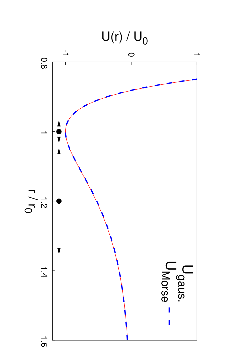
In Fig. 3 the lattice parameter (black dots)and the range of the corresponding lattice fluctuations (double arrows) are also shown for and for K as representative cases of low and high temperature respectively. As we see, the agreement between the Morse potential for Argon and our Gaussian-like potential is practically perfect in all the physical range of spanned at both low and high temperature. This agreement is particularly important since it assures that the results of the variational method for two potentials are indistinguishable.
For the Gaussian-like form of Eq. (18), the smeared potential reads:
| (19) |
In the zero temperature limit () the smeared potential reduces to the bare potential and the elastic constant Eq. (15) to the bare elastic constant . The zero temperature/zero pressure nearest neighbors distance is found by minimizing the classical ground state energy . For the Argon parameters considered in this section we get and which is in good agreement with the experimental value .[37] Note that the value is slightly different from the potential minimum due to the contribution of the second nearest neighbors atoms in the total energy. By increasing the temperature, both the thermal fluctuations and the lattice parameter will have a non trivial dependence on temperature.
III.1 Constant volume
We discuss first the case where the lattice parameter is assumed to be independent of and set to the value , i.e. its value at zero temperature and zero pressure. In this case, the effective elastic constant and the lattice fluctuations can be simply obtained as functions of the temperature by the self-consistent solution of Eqs. (13)-(16), setting the in the lattice sum. The graphical solution of Eq. (16) for three representative temperatures is shown in Fig. 4.

The physical quantity (and hence ) is obtained from the lowest- intersection of the l.h.s function and of the r.h.s. function which is an implicit function of . In the zero temperature limit this solution corresponds to the harmonic limit . On the contrary, the second solution, which is not shown in Fig. 4, starts at from values much higher than the nearest neighbors distance and then it decreases with temperature. It corresponds to a local maximum which does not minimize the free energy and it can be disregarded. The behaviors of and as functions of the temperature are plotted in Fig. 5(a) and in Fig. 5(b).

For a temperature independent volume, above an upper temperature no solution is found (see Fig. 4). The maximum temperature found in this way at for the Argon potential parameters is K, much larger than the experimental melting temperature of the Argon K. Note that the temperature is so high that the linear behavior of (valid for an harmonic crystal) is confined to a very small temperature range (Fig. 5(a)).
We would like to stress that, as remarked in Ref. 30, the breakdown of the SCPT solution at is not signalized by any precursor singular behavior in nor in . On this regards it is worth to analyze explicitly even the behavior of the compressibility as function of the temperature close to the instability temperature where the solution of Eq. (16) disappears. The SCPT solution for the compressibility is thus reported in Fig. 5(c), showing that is well-behaved as the instability temperature at fixed volume is approached. As we are going to see, the behavior of is qualitatively different when the thermal lattice expansion as a function of the temperature at fixed pressure is considered.
III.2 Constant pressure
Before discussing explicitly a system at constant pressure, let us consider first the interatomic distance as an external and tunable parameter in order to gain some useful preliminary insight.
In Fig. 6 we show the behavior of the graphical solution of Eq. (16) for fixed temperature as varying .

We observe that the global effect of increasing the lattice spacing is to reduce the effective elastic constant and to increase thus the mean lattice fluctuations . Thus, according to the Lindemann criterion, we can argue that the breakdown of the solid phase can occur at temperatures lower than the one corresponding to the constant volume case.
In a more compelling way, the physical value of the lattice parameter (or the volume per particle ) is obtained for a given pressure and temperature by inverting the relation , Eq. (17). In Fig. 7 we show as an example the case of zero pressure which simply corresponds to the minimization of the free energy with respect to the volume or, equivalently, to . The evolution of the minimum of at different temperatures shows the thermal expansion of the system at constant pressure .

The corresponding results for the elastic constant and for the thermal fluctuations are reported in Fig. 8(a) and in Fig. 8(b). For comparison in Fig. 8 it is also shown the behavior of and obtained by the self-consistent solution of Eq.(16) as functions of the temperature but assuming three representative fixed lattice spacing . Note that the physical behavior of the elastic constant as a function of the temperature is quite different in the two cases, with a decrease of as a function of at fixed pressure whereas a hardening of is predicted when working at fixed volume

Our calculated data in Fig. 8 (case ) extend up to the spinodal temperature , above which the minimum of as a function of disappears. It is worth noting that such temperature is much lower than related to existence of the self-consistent solution for the lattice fluctuation, and it is of the same order of magnitude of the experimental melting temperature .
Similar results are obtained for fixed finite pressure . As mentioned in Sec. II, the thermal lattice expansion can be traced by minimizing the Gibbs free energy or, equivalently, by inverting Eq. (17) to obtain as a function of and . The behavior of the average fluctuation, the effective elastic constant and the lattice constant are reported in Fig. 9.

Available experimental data of in Argon, in an experimental setup at saturated conditions corresponding to ,[37] are also reported in Fig.9(c), showing an agreement between our calculations and the experimental data. We observe here that increasing the pressure leads to a weaker increase of (weaker decrease of ) as a function of . In other words, the finite pressure leads to an increase of the spinodal temperature at which the solid phase disappears as a metastable solution. We also note that, in similar way as in the analysis at constant volume, neither , , nor the lattice constant show any singular behavior at .
In the present case at constant pressure, however, an additional tool of investigation is provided by the thermal lattice expansion coefficient defined as:
| (20) |
The temperature dependence of at fixed temperature is reported in Fig. 10, showing the singular behavior at . In the inset we plot the thermal expansion coefficient as a function of the reduced variable in a log-log scale, showing a power-law divergence , where was obtained by a fitting procedure.

At the spinodal temperature, the divergence of the lattice expansion coefficient coincides with a singular behavior of the compressibility as it could be guessed by the general thermodynamical relation:[38]
| (21) |
where and are respectively the specific heat at constant pressure and constant volume. Note that a general condition for the lattice stability is the positiveness of the two specific heats ordered as .[39] Using thermodynamical relations, we can rewrite Eq. (21) in the more convenient form
| (22) |
where the internal energy per particle is defined in the Eq. (10), . From Eq. (22), the divergence of at the spinodal temperature implies the divergence of provided the quantity has a finite and regular behavior as approaches . As can be seen from Fig. 11, both and its derivative have a regular behavior for any value of temperature and pressure, pointing out that is proportional to at the spinodal temperature .

IV Phase Diagram
In the previous Sections, we have identified two different mechanisms for the breakdown of the solid state phase within the SCPT model, working respectively at fixed volume and at fixed (moderate) pressure. In the first case the solid phase instability is pointed out by the breakdown of the self-consistent solution of the SCPT at a temperature , with no other evident signature in the thermodynamical properties. On the other hand, a solid state phase is always defined in the second case, which however disappears as a metastable minimum at a spinodal temperature , where the thermal expansion coefficient and the compressibility diverge.
The competition between these two different behaviors can be better clarified analyzing in more details some typical isothermal curves in a wide range of temperatures as shown in Fig. 12. We can thus distinguish between two different pressure ranges.

For high pressures ( with ) we have only one volume solution for given pressure by increasing temperature. In this range the isothermal curves are monotonic as function of pressure, corresponding to a positive isothermal compressibility. This behavior holds true at high temperatures () for any pressure. Increasing the temperature at constant pressure leads to a rapid increase of the volume until the self-consistent solution of the SCPT disappears at the temperature . At we have for instance (Fig. 12).
Below the critical pressure , the isothermal curves are non-monotonic with three possible volume solutions for given pressure, and an intermediate region of negative compressibility (dashed lines in Fig. 12). In this case, the physical more stable solution is the one with smaller volume.[40] Increasing the temperature thus leads to a slight increase of until the first physical solution disappears at the spinodal temperature where the , and the compressibility diverges (for , we have with corresponding to a volume , see Fig. 12). At higher temperature, disregarding phase separated phases, the only physical solution is associated with the large volume cases (for , we have for ). This sudden jump of the volume at reflects thus the divergence of the lattice expansion coefficient at the spinodal temperature.
Increasing further the temperature, even this high volume solution will break due to the breakdown of the self-consistent SCPT solution at a high temperature . As a matter of facts, this kind of instability is driven by the disappearing of the SCPT solution at (the same encountered when working at constant volume) in contrast to the compressibility divergence at .
We can summarize all the above discussion in a compact phase diagram, Fig. 13, which reproduces on a quantitative level the schematic phase diagram sketched in Fig. 2.

The different kinds of instabilities of the solid phase as a function of the pressure are depicted in Fig. 14, where the dashed line represents the spinodal temperature accompanied by the divergence of the lattice expansion coefficient and of the compressibility , while the solid line marks the disappearing of the SCPT solution, as function of temperature, not reflected in any singular behavior of the thermodynamical properties. Note that for , is not defined.

The physical mechanism of the breakdown of the solid phase is determined by the first instability encountered by increasing the temperature. For this is given by the compressibility divergence at . For no thermodynamical instability is encountered and the unique instability of the solid phase is associated with .
Fig.14 permits also to clarify in simple terms why the mechanical instability at constant volume occurs at much higher temperature and with different phenomenology than at constant pressure. Considering for simplicity a constant volume (), increasing the temperature is indeed associated with an effective increase of . Such increase is however negligible on the scale , so that the first encountered solid phase instability occurs at much higher temperatures, as shown in the inset, and it is related to the SCPT breakdown at .
V Discussion and conclusions
In this paper we have revisited the self-consistent phonon theory (SCPT) to analyze the mechanism of the mechanical instability of an overheated metastable solid at finite pressure.
Within this approach, we have predicted that two different instabilities are possible for the mechanical melting. They occur at very different temperatures, depending whether working at fixed volume or pressure. In the first case the instability of the solid phase occurs at rather high temperatures and it is associated with a breakdown of the SCPT solution at , not reflected in any singular behavior of the thermodynamical quantities. On the other hand, the mechanical instability approached at fixed pressure, for pressures smaller than a critical pressure , can be properly interpreted in terms of a spinodal temperature at which the solid phase, always defined, disappears as a metastable minimum. In the latter case the mechanical instability is reflected in the divergence of the thermal compressibility as well as in the divergence of the lattice expansion coefficient at . Such kind of spinodal instability disappears for , where only the instability at driven by the breakdown of the SCPT solution remains. The value of is found to be of order where is the energy minimum of the pair potential and the lattice spacing. For the weakly bound rare-gas solids we have of the order of few meVs, corresponding thus to a critical of the order of some MPa.
For a quantitative comparison with real systems, in this paper we have mainly focused on the specific case of an Argon classical solid where intensive theoretical and experimental investigation have been performed in literature (as example, see Ref. 22 and references therein).
Similar analysis can be however carried out in a simple way as well for other rare-gas solids (Xe, Ne, Kr). The results are collected in Table 1 where we report the theoretical and compared also with the experimental melting temperature . As we can see, is systematically much lower than and it is of the same order of magnitude of the experimental melting temperature . Inclusion of higher order anharmonic terms[41] and the development of models beyond the Einstein one[35, 42] (i.e. taking into account the full phonons dispersion) might further reduce towards the empirical range for overheating .[20]
| (K) | (K) | (K) | ||||
|---|---|---|---|---|---|---|
| Ne | 25 | 2450 | 69 | |||
| Ar | 83 | 9747 | 228 | |||
| Kr | 116 | 18986 | 317 | |||
| Xe | 161 | 21662 | 445 |
Such analysis points out that taking into account the lattice expansion is of fundamental importance not only for a proper quantitative estimate of the instability temperature of the solid phase, but also for revealing the different instability mechanisms associated or not associated with a singular behavior of the thermodynamical properties.
Acknowledgements.
The authors acknowledges useful discussions with S. Ciuchi. Critical reading of the manuscript by M. Holzmann is appreciated.References
- [1] J. Daeges, H. Gleiter, and J. H. Perepezko, Phys. Lett. A 119, 79 (1986).
- [2] L. Gråbæk, J. Bohr, H. H. Andersen, A. Johansen, E. Johnson, L. Sarholt-Kristensen, and I. K. Robinson, Phys. Rev. B 45, 2628 (1992).
- [3] Z. H. Zhang and H. E. Elsayed-Ali, Surf. Sci. 405, 271 (1998).
- [4] L. Zhang, ZḢ. Jin, L. H. Zhang, M. L. Sui, and K. Lu, Phys. Rev. Lett. 85, 1484 (2000).
- [5] S.-N. Luo and T. J. Ahrens, Appl. Phys. Lett. 82, 1836 (2003).
- [6] K. Sokolowski-Tinten et al., Nature 422, 287 (2003).
- [7] B. J. Siwick, J. R. Dwyer, R. E. Jordan, and R. J. Dwayne Miller, Science 302, 1382 (2003).
- [8] H. Iglev, M. Schmeisser, K. Simeonidis, A. Thaller, and A. Laubereau, Nature 439, 183 (2006).
- [9] Q. S. Mei and K. Lu, Prog. Mater. Sci. 52, 1175 (2007).
- [10] Y. Feng, J. Goree, and B. Liu, Phys. Rev. Lett. 100, 205007 (2008).
- [11] R.W. Cahn, Nature 334, 17 (1988); ibid. 342, 619 (1989); ibid. 413, 582 (2001).
- [12] J. G. Dash, Rev. Mod. Phys. 71, 1737 (1999).
- [13] H. Löwen, Phys. Rep. 237, 249 (1994).
- [14] F. A. Lindemann, Z. Phys. 11, 609 (1910).
- [15] M. Born, J. Chem. Phys. 7, 591 (1939); Proc. Cambridge Philos. Soc. 36, 160 (1940).
- [16] H. J. Fecht and W. L. Johnson, Nature 334, 50 (1988).
- [17] J. L. Tallon, Nature 342, 658 (1989).
- [18] L. L. Boyer, Phase Transitions 5, 1 (1985).
- [19] Z. H. Jin, P. Gumbsch, K. Lu, and E. Ma, Phys. Rev. Lett. 87, 055703 (2001).
- [20] S.-N. Luo, T. J. Ahrens, T. Çağin, A. Strachan, W. A. Goddard, and D. C. Swift, Phys. Rev. B 68, 134206 (2003).
- [21] M. Forsblom and G. Grimvall, Nat. Mater. 4, 388 (2005).
- [22] S.-N. Luo, L. Zheng, A. Strachan, and D. C. Swift, J. Chem. Phys. 126, 034505 (2007).
- [23] P. F. Choquard, The Anharmonic Crystal (Benjamin, New York 1967) Chap.7.
- [24] N. S. Gillis, N. R. Werthamer, and T. R. Koehler, Phys. Rev. 165, 951 (1968).
- [25] N. S. Gillis, T. R. Koehler, and N. R. Werthamer, Phys. Rev. 175, 1110 (1968).
- [26] A. A. Kugler, Annals of Physics 53, 133 (1969).
- [27] M. L. Klein, G. K. Horton, and V. V. Goldman, Phys. Rev. B 2, 4995 (1970).
- [28] N. S. Gillis and T. R. Koehler, Phys. Rev. Letts. 29, 369 (1972).
- [29] T. Matsubara, Y. Iwase, and A. Momokita, Prog. Theor. Phys. Japan 58, 1102 (1977).
- [30] L. Pietronero and E. Tosatti, Solid State Commun. 32, 255 (1979).
- [31] M. Hasegawa, K. Hoshino, and M. Watabe, J. Phys. F: Metal Phys. 10, 619 (1980).
- [32] C. S. Jayanthi, E. Tosatti, and L. Pietronero, Phys. Rev. B 31, 3456 (1985).
- [33] C. S. Jayanthi, E. Tosatti, and A. Fasolino, Phys. Rev. B 31, 470 (1985).
- [34] C. Gong, D. Xing, A. Holz, and J. Pang, Phys. Rev. B 36, 5517 (1987).
- [35] L.K. Moleko and H.R. Glyde, Phys. Rev. B 27, 6019 (1983).
- [36] An exception is the work of Ref. 35, where the authors took into account the thermal dilatation of the lattice by the experimental data but, for temperatures beyond the melting temperature , they assumed the lattice spacing frozen at the value .
- [37] O. G. Peterson, D. N. Batchelder, and R. O. Simmons, Phys. Rev. 150, 703 (1966).
- [38] K. Huang, Statistical Mechanics 2nd ed. (Wiley, New York 1987).
- [39] L.D. Landau and E. M. Lifshitz, Statistical Physics, 3rd ed. (Pergamon Press, Oxford 1980) Chap. 2.
- [40] A Maxwell construction, corresponding to a phase separation between coexisting regions of stable solid phases with different volumes is in principle possible in this framework. The analysis of such possibility goes however beyond the purposes of the present work, which is aimed to underlying the different breakdown mechanisms of the solid phase within the SCPT operative at constant and at constant .
- [41] A. Paskin, A.-M. Llois de Kreiner, K. Shukla, D. O. Welch, and G. J. Dienes, Phys. Rev. B 25, 1297 (1982).
- [42] R. C. Shukla and E. R. Cowley, Phys. Rev. B 58, 2596 (1998).