Sublinear randomized algorithms for skeleton decompositionsThanks: Dated April 2012.
Abstract
Let be a by matrix. A skeleton decomposition is any factorization of the form where comprises columns of , and comprises rows of . In this paper, we consider uniformly sampling rows and columns to produce a skeleton decomposition. The algorithm runs in time, and has the following error guarantee. Let denote the -norm. Suppose where each have orthonormal columns. Assuming that are incoherent, we show that with high probability, the approximation error will scale with or better. A key step in this algorithm involves regularization. This step is crucial for a nonsymmetric as empirical results suggest. Finally, we use our proof framework to analyze two existing algorithms in an intuitive way.
Acknowledgments
JC is supported by the A*STAR fellowship from Singapore. LD is supported in part by the National Science Foundation and the Alfred P. Sloan foundation. We would also like to thank the referees for making many valuable suggestions.
1 Introduction
1.1 Skeleton decompositions
This paper is concerned with the decomposition known as the matrix skeleton11 1 The term “skeleton” may refer to other factorizations. Instead of , we can have where are arbitrary and matrices [14]. As space is needed to store , this representation does not seem as appealing. Nevertheless, it is numerically more stable and has found several applications [25]. When where are matrices, we can approximate as , as , where has columns of and has rows of . Thus, , effectively replacing with the matrix . Bremer calls a skeleton and uses it to approximate scattering matrices [7]., pseudo-skeleton [22], or CUR factorization [29, 18].
For the rest of the paper, we adopt the following Matlab-friendly notation: given , will denote the restriction of to columns indexed by , and will denote the restriction of to rows indexed by . A skeleton decomposition of is any factorization of the form
In general, a rank- approximation of takes up space. The major advantage of the skeleton decomposition is that it may require only space. Consider the case where ’s entries can be specified by a function in closed form. Then the skeleton decomposition is fully specified by as well as the two index sets and . In addition, row and columns from the original matrix may carry more physical significance than linear combinations thereof.
There are important examples where the full matrix itself is not low rank but can be partitioned into blocks each of which has low numerical rank. One example is the Green’s function of elliptic operators with mild regularity conditions [4]. Another example is the amplitude factor in certain Fourier integral operators and wave propagators [11, 16]. Algorithms that compute good skeleton representations can be used to compress such matrices.
1.2 Overview
Algorithm 1.
Skeleton via uniform sampling, algorithm.
Input: A matrix , and user-defined parameters and .
Output: A skeleton representation with rows and columns.
Steps:
1.
Uniformly and independently select columns to form .
2.
Uniformly and independently select rows to form .
3.
Compute the SVD of . Remove all the components with singular values less than . Treat this as a perturbation of such that and .
4.
Compute . (In Matlab, Z=pinv(A(R,C),delta).)
5.
Output .
In this paper, we consider uniformly sampling rows and columns of to build a skeleton decomposition. After obtaining this way, we compute the middle matrix as the pseudoinverse of with thresholding or regularization. See Algorithm 1 for more details. Suppose where have orthonormal columns. Assuming that are incoherent, we show in Theorem 2 that the -norm approximation error is bounded by with high probability. We believe that this is the first known relative error bound in the -norm for a nonsymmetric .
The idea of uniformly sampling rows and columns to build a skeleton is not new. In particular, for the case where is symmetric, this technique may be known as the Nystrom method22 2 In machine learning, the Nystrom method can be used to approximate kernel matrices of support vector machines, or the Laplacian of affinity graphs, for instance.. The skeleton used is , which is symmetric, and its -norm error is recently analyzed by Talwalkar [37] and Gittens [21]. Both papers make the same assumption that are incoherent. In fact, Gittens arrives at the same relative error bound as us.
Nonetheless, our results are more general. They apply to nonsymmetric matrices that are low rank in a broader sense. Specifically, when we write , is not necessarily diagonal and are not necessarily the singular vectors of . This relaxes the incoherence requirement on . Furthermore, in the physical sciences, it is not uncommon to work with linear operators that are known a priori to be almost diagonalized by the Fourier basis or related bases in harmonic analysis. These bases are often incoherent. One example is an integral operator with a smooth kernel. See Section 4 for more details.
The drawback of our results is that it requires us to set an appropriate regularization parameter in advance. Unfortunately, there is no known way of estimating it fast, and this regularization step cannot be skipped. In Section 4.1, we illustrate with a numerical example that without the regularization, the approximation error can blow up in a way predicted by Theorem 2.
Finally, we also establish error bounds for two other algorithms. We shall postpone the details.
1.3 Some previous work
Before presenting our main results, we like to provide a sample of some previous work. The well-informed reader may want to move on.
The precursor to the skeleton decomposition is the interpolative decomposition [14], also called the column subset selection problem [20]. An interpolative decomposition of is the factorization for some . The earliest work on this topic is probably the pivoted QR algorithm by Businger, Golub [8] in 1965. In 1987, Chan [12] introduced the Rank Revealing QR (RRQR); a sequence of improved algorithms and bounds followed [19, 26, 31, 23]. RRQR algorithms can also be used to compute skeletons [28].
An early result due to Goreinov et al. [22] says that for any , there exists a skeleton such that in the -norm, . Although the proof is constructive, it requires computing the SVD of , which is much more costly than the algorithms considered in this paper. An useful idea here is to maximize the volume or determinant of submatrices. This idea is also used to study RRQRs [13], and may date back to the proof of Auerbach’s theorem [35], interpolating projections [33] etc.
One way of building a skeleton is to iteratively select good rows and columns based on the residual matrix. This is known as Cross Approximation. As processing the entire residual matrix is not practical, there are faster algorithms that operate on only a small part of the residual, e.g., Adaptive Cross Approximation [2, 3], Incomplete Cross Approximation [39]. These methods are used to compress off-diagonal blocks of “asymptotically smooth” kernels. The results of this paper will also apply to such smooth kernels. See Section 4.2.
Another way of building a skeleton is to do random sampling, which may date back to [20]. One way of sampling is called “subspace sampling” [29, 18] by Drineas et al. If we assume that the top singular vectors are incoherent, then a result due to Rudelson, Vershynin [34] implies that uniform sampling of rows and columns, a special case of “subspace sampling”, will produce a good skeleton representation . However, it is not clear how the middle matrix can be computed in sublinear time. In this paper, the skeleton we analyze resembles , which can be computed in time.
1.4 Preliminaries
The matrices we consider in this paper take the form
| (1) |
where and are unitary matrices, with columns being “spread”, and the blocks and are in some sense small. By “spread”, we mean -coherent.
Definition 1.
Let be a matrix with orthonormal columns. Denote . We say is -coherent if .
To formalize “small”, let , and consider that
| (2) |
By tolerating an error in the -norm, can be represented using only data. Note that is equivalent to up to constants. To prevent clutter, we have suppressed the dependence on from the definitions of etc.
If (1) is the SVD of , then . It is good to keep this example in mind as it simplifies many formulas that we see later.
An alternative to is
| (3) |
In other words, is the norm of reshaped into a vector. We know . The reason for introducing is that it is common for to decay rapidly such that . For such scenarios, the -norm error may grow much slower with .
1.5 Main result
Our main contribution is the error analysis of Algorithm 1. The problem with the algorithm is that it does not always work. For example, if and , then is going to be zero most of the time, and so is . Hence, it makes sense that we want to be “as nonsingular as possible” so that little information is lost. In particular, it is well-known that if are -coherent, i.e., spread, then sampling rows will lead to being well-conditioned33 3 The requirement that can be relaxed in at least two ways. First, all we need is that which would allow a few entries of every row of to be big. Second, if only a few rows of violate this condition, we are still fine as explained in [1]..
Here is our main result. It is proved in Section 2.
Theorem 2.
Minimize the RHS of (4) and (5) with respect to . For (4), pick so that
| (6) |
For (5), pick so that
| (7) |
Here are some possible scenarios where and (7) is much better than (6):
- •
The entries of decay exponentially or there are only nonzero entries as increases. Then .
- •
Say and (1) is the SVD of . Suppose the singular values decay as . Then .
One important question remains: what is ? Unfortunately, we are not aware of any algorithm that can accurately estimate . Here is one possible heuristic for choosing for the case where (1) is the SVD. Imagine . As we will see, the singular values of are likely to be on the order of . Therefore, we may pretend that .
Another approach is to begin with a big , run the algorithm, check , divide by two and repeat the whole process until the error does not improve. However, calculating is expensive and we will need other tricks. This is an open problem.
The algorithm is probably the fastest algorithm for computing skeleton representations that one can expect to have. If we do more work, what can we gain? In Section 3, we sketch two such algorithms. The first one samples rows, columns, then reduce it to exactly rows, columns using RRQR, with a -norm error of . It is similar to what is done in [5]. In the second algorithm, we uniformly sample rows to get , then run RRQR on to select columns of . The overall error is . This is similar to the algorithm proposed by Tygert, Rokhlin et al. [28, 40].
1.6 More on incoherence
Haar unitary matrices are -coherent [17, Theorem VIII.1], that is if we draw uniformly from the special orthogonal group, it is very likely that they are incoherent. This means Algorithm 1 will work well with .
If either or is not -coherent, we can use an old trick in compressed sensing [1]: multiply them on the left by the unitary Fourier matrix with randomly rescaled columns. This has the effect of “blending up” the rows of . The following is an easy consequence of Hoeffding’s inequality, and the proof is omitted.
Proposition 3.
Let with orthonormal columns. Let where are independent random variables such that and . Let be the unitary Fourier matrix and for some . Define . Then with probability at least
In words, no matter what is, would be -coherent whp. Hence, we can write a simple wrapper around Algorithm 1.
- 1.
Let where are diagonal matrices with independent entries that are with equal probability.
- 2.
Feed to the algorithm and obtain .
- 3.
It follows that .
The output is not a skeleton representation, but the amount of space needed is which is still better than . However, the algorithm may no longer run in sublinear time.
2 Error estimates for algorithm
2.1 Notation
are both column selector matrices. They are column subsets of permutation matrices. The subscripts “” and “” denote a row subset and a column subset respectively, e.g., and , while is a row and column subset of . Transposes and pseudoinverses are taken after the subscripts, e.g., .
2.2 Two principles
Our proofs are built on two principles. The first principle is well-known in compressed sensing, and dates back to Rudelson [34] in 1999. Intuitively, it says:
Let be a matrix with orthonormal columns. Let be a random row subset of . Suppose is -coherent with , and . Then with high probability, is like an isometry.
To be precise, we quote [38, Lemma 3.4]. (Note that their is our .)
Theorem 4.
Let with orthonormal columns. Suppose is -coherent and for some . Let be a random -row subset of . Each row of is sampled independently, uniformly. Then
and
If and and , then
| (8) |
We will use (8) later. Let us proceed to the second principle, which says
Let be a nonrandom index set. If is small , then is also small, provided that we have control over and for some unitary matrix .
The motivation is as follows. If we ignore the regularization step, then what we want to show is that . But when we take row and column restrictions on both sides, we have trivially . Hence, we desire a mechanism to go backwards, that is to infer that “ is small” from “ is small.” We begin by inferring that “ is small” from “ is small”.
Lemma 5.
Let and be a unitary matrix such that has columns. Select rows of to form . Assume has full column rank. Then
Proof.
Note that . Now,
∎
Lemma 5 can be extended in two obvious ways. One, we can deduce that “ is small if is small.” Two, we can deduce that “ is small if is small.” This is what the next lemma says. The proof is a straightforward modification of the proof of Lemma 5 and shall be omitted.
Lemma 6.
Let and and be unitary matrices such that each has columns. Select rows and columns indexed by respectively. Assume have full column rank. Then
and
We conclude this section with a useful corollary. It says that if is a good low rank approximation of for some , then may also be a good low rank approximation of .
Corollary 7.
Let and . Let be a unitary matrix such that has columns. Let where . Assume has full column rank. Let be the identity. Then
In particular, if is the orthogonal projection , then
| (9) |
Proof.
To get the first inequality, apply Lemma 5 to . The second inequality is immediate from the first inequality since . ∎
2.3 Proof of Theorem 2
Let and . To prove the first part of Theorem 2, that is (4), apply the first principle or Theorem 4. From (8), it is clear that , , , hold simultaneously with probability at least .
For the second part of Theorem 2, that is (5), we need to refine (1) as follows. Let and where and has columns, and have columns. Note that , , where are defined in (1). Rewrite (1) as
| (10) |
By applying Theorem 4 to every , and doing a union bound, we see that with probability at least , we will have , , , for all .
The rest of the proof is deterministic.
Suppose the SVD of is . Define another vector such that if , zero otherwise. Let . The skeleton decomposition we return is . The point of adding to is to avoid “inverting” singular values that are less than .
Define the matrix such that and all other entries are zeros. Now, let so that . The skeleton returned is . By construction, and .
Our objective is to bound . Split this up by a perturbation argument.
| (11) |
It remains to bound using the second principle. Intuitively, cannot be too much bigger than .
By Lemma 5,
By the first principle, the following holds whp:
| (12) |
The same argument works for . Whp,
| (13) |
Bounding requires more work, but the basic ideas are the same. Recall that the second principle suggests that cannot be too much bigger than . Applying Lemma 6 with being yields
which is bounded by
We have paired with , and with because the first principle implies that their products are whp. That means
We have dropped because it is dominated by . (13) and (12) can be used to control and . Before doing that, we want to replace with in all the other terms. This will introduce some extra ’s. For example, . Doing the same for other terms, we have that is whp
Several terms can be dropped in the notation, for example and . We shall also plug in the estimates on and , from (13) and (12). This leads to
Collect the terms by their factors and drop the smaller terms to obtain that whp, is
| (14) |
We now have control over all three terms . Substitute (12), (13), (14) into (11). As the RHS of (14) dominates multiplied by the RHS of (12), (13), we conclude that whp, is also bounded by the RHS of (14).
To obtain the basic bound, (4), we note that all the “normed terms” on the RHS of (14), e.g., and , are bounded by . It follows that whp, .
Recall (10). Consider . See that
Recall that at the beginning of the subsection, we show that whp, and for all . Recall the definition of in (3). It follows that whp,
Apply the same argument to other terms on the RHS of (14), e.g., and whp. Mnemonically, a in the subscript leads to a and a in the subscript leads to a .
3 Two other algorithms
3.1 Second algorithm
Algorithm 2 returns a skeleton with exactly rows and columns. First, randomly select rows and columns, then trim down to columns and rows by performing RRQR on and . For dense matrices, the most expensive step is the multiplication of by . However, for structured matrices, the most expensive step of Algorithm 2 may be the RRQR factorization of and and the inversion of , which take time. The overall running time is where is the cost of matrix-vector multiplication, but for convenience, we refer to this as the algorithm.
Algorithm 2.
algorithm
Input: Matrix .
Output: A skeleton representation with exactly rows and columns.
Steps:
1.
Uniformly and independently select columns to form .
2.
Uniformly and independently select rows to form .
3.
Run RRQR on to select columns and form . This takes time and space.
4.
Run RRQR on to select rows and form . This takes time and space.
5.
Compute . This takes time and space, where is the time needed to apply to a vector.
6.
Output .
It can be shown that once are fixed, the choice of is optimal in the Frobenius norm (but not in the -norm), that is . Not surprisingly, we have a better error estimate.
Theorem 8.
Proof.
Many algorithms that use the skeleton , e.g. [29], seek to select columns such that is small. Here, we further select out of columns, which is also suggested in [5]. Their -norm error estimate is where is the optimal rank approximation to . In general , so our bound is a factor better. Our proof is also more straightforward. Nevertheless, we make the extra assumption that are incoherent.
3.2 Third algorithm
Consider the case where only is -coherent. See Algorithm 3. It computes a skeleton with rows and columns in time. Intuitively, the algorithm works as follows. We want to select columns of but running RRQR on is too expensive. Instead, we randomly choose rows to form , and select our columns using the much smaller matrix . This works because is assumed to be -coherent and choosing almost any rows will give us a good sketch of .
Algorithm 3.
algorithm
Input: Matrix .
Output: A skeleton representation with rows and columns.
Steps:
1.
Uniformly and independently select rows to form .
2.
Run RRQR on . Obtain where contains columns of . This takes time and space.
3.
Compute . This takes time and space.
4.
Output .
Theorem 9.
Proof.
We perform RRQR on to obtain where and indexes the selected columns. We want to use the second principle to “undo the row restriction” and infer that , the output of Algorithm 3. We now fill in the details.
If is not incoherent and we fix it by multiplying on the left by a randomized Fourier matrix (cf. Section 1.6), then we arrive at the algorithm in [28]. The linear algebraic part of their proof combined with the first principle will lead to the same bounds. What we have done here is to decouple the proof into three simple parts: (1) show that is incoherent, (2) use the first principle to show that is “sufficiently nonsingular”, (3) use the second principle to finish up the linear algebra.
3.3 Comparing the three algorithms
Here is a summary of the three algorithms studied in this paper. Assume .
| No. rows | No. columns | Error in -norm | Running time | Memory | |
|---|---|---|---|---|---|
| Algorithm 1 | |||||
| Algorithm 2 | |||||
| Algorithm 3 |
Suppose has structure and . If we can tolerate a factor in the running time and memory usage, then Algorithm 2 is the method of choice. Otherwise, we recommend using Algorithm 1. It is much faster and even though Theorem 2 suggests that the error grows with , we believe that in practice, the error usually grows with .
Suppose is dense and has no structure. In this case, Algorithm 2 is too slow. As for Algorithm 3, it runs significantly slower than Algorithm 1 and its error bounds are not any better. However, if we do not want to worry about setting the parameter , we will prefer to use Algorithm 3.
4 Examples
For this section, we consider only Algorithm 1, the algorithm.
4.1 Toy example
Let where are unitary Fourier matrices and is a diagonal matrix of singular values. Note that every entry of is of magnitude and are -coherent.
For the first experiment, is and . We also pick the first singular values to be logarithmically spaced between and . In each trial, we randomly pick rows and columns and measure . The only parameters being varied are and .
From (4) in Theorem 2, we may expect that when variables such as are fixed,
| (16) |
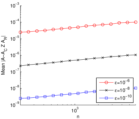
Consider a plot of versus on a log-log scale. According to the above equation, when , the first term dominates and we expect to see a line of slope , and when , and we expect to see a line of slope . Indeed, when we plot the experimental results in Figure 1, we see a right-angled -curve.
A curious feature of Figure 1 is that the error curves behaves like a staircase. As we decrease , the number of different error levels decrease proportionally. A possible explanation for this behavior is that the top singular vectors of match those of , and as increases from to for some small , smaller components will not be inverted and the error is all on the order of .
For the second experiment, we use the same matrix but vary instead of . We fix , and . There are three different runs with . The results are plotted in Figure 2. They suggest that the error scales with , which is better than (6).
4.2 Smooth kernel
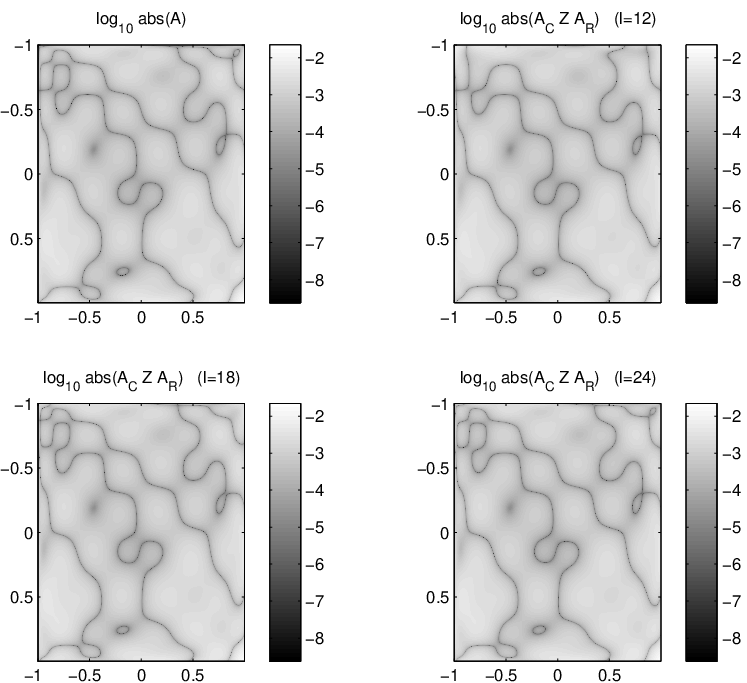
Consider a 1D integral operator with a kernel that is analytic on . Define as where the nodes and are uniformly spaced in . First, suppose where is the -th Chebyshev polynomial and is the random Gaussian matrix, i.e., noise. The coefficients ’s are chosen such that . Pick and slowly increase , the number of rows and columns sampled by the algorithm. As shown in Figure 3, the skeleton representation converges rapidly to as we increase .
Next, consider . Let and pick to normalize . We then plot the empirical mean of the error of the algorithm against on the left of Figure 4. Notice that the error decreases exponentially with .
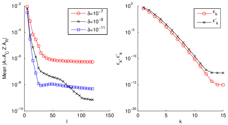
To understand what is happening, imagine that the grid is infinitely fine. Let be Legendre polynomials. Recall that these polynomials are orthogonal on . Define the matrices as and . Assume the ’s are scaled such that are unitary. It is well-known that if we expand in terms of Chebyshev polynomials or Legendre polynomials [6] or prolate spheroidal wave functions [41], the expansion coefficients will decay exponentially. This means that the entries of should decay exponentially away from the topleft corner and (cf. (2) and (3)). We confirm this by plotting versus on the right of Figure 4. The actual used to obtain this plot are obtained by evaluating the Legendre polynomials on the uniform grid and orthonormalizing. It can be verified that the entries of are of magnitude which implies a coherence , independent of . The implication is that the algorithm will continue to perform well as increases.
As increases, we can apply Theorem 2 with a larger . Since decrease exponentially, the error should also decrease exponentially. However, as increases beyond , stagnates and nothing can be gained from increasing . In general, as decreases, we should pick a smaller . But when , choosing a smaller does not help and may lead to worse results due to the instability of pseudoinverses and floating point errors. This is evident from Figure 4.
Platte, Trefethen, Kuijlaars [32] state that if we sample on a uniform grid, the error of any stable approximation scheme cannot decrease exponentially forever. In this example, the random selection of columns and rows correspond to selecting interpolation points randomly from a uniform grid, and serves as a regularization parameter of our approximation scheme. The method is stable, but we can only expect an exponential decrease of the error up to a limit dependent on .
4.3 Fourier integral operators
In [11], Candes et al. consider how to efficiently apply 2D Fourier integral operators of the form
where is the Fourier transform of , is a smooth amplitude function and is a smooth phase function that is homogeneous, i.e., for any . Say there are points in the space domain and also the frequency domain.
The main idea is to split the frequency domain into wedges, Taylor expand about where indexes a wedge, and observe that the residual phase is nonoscillatory. Hence, the matrix can be approximated by a low rank matrix, i.e., can be written as where , the separation rank, is independent of . By switching order of summations, the authors arrive at algorithms for both the preprocessing and the evaluation steps. See [11] for further details.
What we are concerned here is the approximate factorization of . This is a by matrix since there are points in the space domain and points in one wedge in the frequency domain. In [11], a slightly different algorithm is proposed.
- 1.
Uniformly and randomly select rows and columns to form and .
- 2.
Perform SVD on . Say where are unitary and , a user specified parameter.
- 3.
Return the low rank representation .
In the words of the authors, “this randomized approach works well in practice although we are not able to offer a rigorous proof of its accuracy, and expect one to be non-trivial” [11]. We believe this is because does satisfy the assumptions of this paper. See (1), (2).
To see why, let be a perturbation of such that and . Since is invertible, the output can be rewritten as
It is easy to adapt the proof of Theorem 2 to bound — just replace (11) with the following. The rest of the proof is the same.
An important subclass of Fourier integral operators is pseudodifferential operators. These are linear operators with pseudodifferential symbols that obey certain smoothness conditions [36]. In Discrete Symbol Calculus [15], a similar randomized algorithm is used to derive low rank factorizations of such smooth symbols. It is likely that the method works well here in the same way as it works well for a smooth kernel as discussed in the previous section.
References
- [1] H. Avron, P. Maymounkov, and S. Toledo, Blendenpik: Supercharging LAPACK’s least-squares solver, SIAM Journal on Scientific Computing, 32 (2010), pp. 1217–1236.
- [2] M. Bebendorf, Approximation of boundary element matrices, Numerische Mathematik, 86 (2000), pp. 565–589.
- [3] M. Bebendorf and R. Grzhibovskis, Accelerating Galerkin BEM for linear elasticity using adaptive cross approximation, Mathematical Methods in the Applied Sciences, 29 (2006), pp. 1721–1747.
- [4] M. Bebendorf and W. Hackbusch, Existence of H-matrix approximants to the inverse FE-matrix of elliptic operators with -coefficients, Numerische Mathematik, 95 (2003), pp. 1–28.
- [5] C. Boutsidis, M.W. Mahoney, and P. Drineas, An improved approximation algorithm for the column subset selection problem, in Proceedings of the twentieth Annual ACM-SIAM Symposium on Discrete Algorithms, Society for Industrial and Applied Mathematics, 2009, pp. 968–977.
- [6] J.P. Boyd, Chebyshev and Fourier spectral methods, Dover Pubns, 2001.
- [7] J. Bremer, A fast direct solver for the integral equations of scattering theory on planar curves with corners, (2011).
- [8] P. Businger and G.H. Golub, Linear least squares solutions by Householder transformations, Numerische Mathematik, 7 (1965), pp. 269–276.
- [9] E.J. Candès and B. Recht, Exact matrix completion via convex optimization, Foundations of Computational Mathematics, 9 (2009), pp. 717–772.
- [10] E. Candes and J. Romberg, Sparsity and incoherence in compressive sampling, Inverse problems, 23 (2007), p. 969.
- [11] E. J. Candès, L. Demanet, and L. Ying, Fast computation of Fourier integral operators, SIAM Journal on Scientific Computing, 29 (2007), pp. 2464–2493.
- [12] T.F. Chan, Rank revealing QR factorizations, Linear Algebra and Its Applications, 88 (1987), pp. 67–82.
- [13] S. Chandrasekaran and I.C.F. Ipsen, On rank-revealing factorisations, SIAM Journal on Matrix Analysis and Applications, 15 (1994), p. 592.
- [14] H. Cheng, Z. Gimbutas, P.G. Martinsson, and V. Rokhlin, On the compression of low rank matrices, SIAM Journal on Scientific Computing, 26 (2005), pp. 1389–1404.
- [15] L. Demanet and L. Ying, Discrete Symbol Calculus, SIAM Review, 53 (2011), pp. 71–104.
- [16] , Fast wave computation via Fourier integral operators, submitted, (2011).
- [17] D.L. Donoho and X. Huo, Uncertainty principles and ideal atomic decomposition, Information Theory, IEEE Transactions on, 47 (2001), pp. 2845–2862.
- [18] P. Drineas, M.W. Mahoney, and S. Muthukrishnan, Relative-error CUR matrix decompositions, SIAM Journal on Matrix Analysis and Applications, 30 (2008), pp. 844–881.
- [19] L.V. Foster, Rank and null space calculations using matrix decomposition without column interchanges, Linear Algebra and its Applications, 74 (1986), pp. 47–71.
- [20] A. Frieze, R. Kannan, and S. Vempala, Fast Monte-Carlo algorithms for finding low-rank approximations, Journal of the ACM (JACM), 51 (2004), pp. 1025–1041.
- [21] A. Gittens, The spectral norm error of the naive Nystrom extension, Arxiv preprint arXiv:1110.5305, (2011).
- [22] S.A. Goreinov, E.E. Tyrtyshnikov, and N.L. Zamarashkin, A theory of pseudoskeleton approximations, Linear Algebra and its Applications, 261 (1997), pp. 1–21.
- [23] M. Gu and S.C. Eisenstat, Efficient algorithms for computing a strong rank-revealing QR factorization, SIAM Journal on Scientific Computing, 17 (1996), pp. 848–869.
- [24] N. Halko, P.G. Martinsson, and J.A. Tropp, Finding structure with randomness: Probabilistic algorithms for constructing approximate matrix decompositions, SIAM Review, 53 (2011), pp. 217–288.
- [25] K.L. Ho and L. Greengard, A fast direct solver for structured linear systems by recursive skeletonization, 2011.
- [26] Y.P. Hong and C.T. Pan, Rank-revealing QR factorizations and the singular value decomposition, Mathematics of Computation, 58 (1992), pp. 213–232.
- [27] R.A. Horn and C.R. Johnson, Topics in matrix analysis, Cambridge Univ Pr, 1994.
- [28] E. Liberty, F. Woolfe, P.G. Martinsson, V. Rokhlin, and M. Tygert, Randomized algorithms for the low-rank approximation of matrices, Proceedings of the National Academy of Sciences, 104 (2007), p. 20167.
- [29] M.W. Mahoney and P. Drineas, CUR matrix decompositions for improved data analysis, Proceedings of the National Academy of Sciences, 106 (2009), p. 697.
- [30] S. Negahban and M.J. Wainwright, Restricted strong convexity and weighted matrix completion: Optimal bounds with noise, Arxiv preprint arXiv:1009.2118, (2010).
- [31] C.T. Pan and P.T.P. Tang, Bounds on singular values revealed by QR factorizations, BIT Numerical Mathematics, 39 (1999), pp. 740–756.
- [32] R.B. Platte, L.N. Trefethen, and A.B.J. Kuijlaars, Impossibility of fast stable approximation of analytic functions from equispaced samples, SIAM Rev, 53 (2011), pp. 308–318.
- [33] K.H. Price and E.W. Cheney, Minimal projections, Approximation Theory, A. Talbot., ed., Academic Press, NewYork, (1970), pp. 261–289.
- [34] M. Rudelson, Random vectors in the isotropic position, Journal of Functional Analysis, 164 (1999), pp. 60–72.
- [35] A.F. Ruston, Auerbach’s theorem and tensor products of Banach spaces, in Mathematical Proceedings of the Cambridge Philosophical Society, vol. 58, Cambridge Univ Press, 1962, pp. 476–480.
- [36] M.A. Shubin, Pseudodifferential operators and spectral theory, Springer Verlag, 2001.
- [37] A. Talwalkar and A. Rostamizadeh, Matrix coherence and the Nystrom method, Arxiv preprint arXiv:1004.2008, (2010).
- [38] J.A. Tropp, Improved analysis of the subsampled randomized hadamard transform, Advances in Adaptive Data Analysis, 3 (2011), pp. 115–126.
- [39] E. Tyrtyshnikov, Incomplete cross approximation in the mosaic-skeleton method, Computing, 64 (2000), pp. 367–380.
- [40] F. Woolfe, E. Liberty, V. Rokhlin, and M. Tygert, A fast randomized algorithm for the approximation of matrices, Applied and Computational Harmonic Analysis, 25 (2008), pp. 335–366.
- [41] H. Xiao, V. Rokhlin, and N. Yarvin, Prolate spheroidal wavefunctions, quadrature and interpolation, Inverse Problems, 17 (2001), p. 805.