跳到论文正文
W Papers独立论文阅读器 arXiv:1110.4091 论文正文 计算阅读时间 · 0%
引用这篇论文根据当前论文元数据生成,正式投稿前建议核对。


License: arXiv.org perpetual non-exclusive license
arXiv:1110.4091v1 [cond-mat.str-el] 18 Oct 2011

Two-orbital Schwinger Boson Representation of Spin-One: Application to a Non-abelian Spin Liquid with Quaternion Gauge Field

Fa Wang Affiliation: Department of Physics, Massachusetts Institute of Technology, Cambridge, Massachusetts 02139, USA    Cenke Xu Affiliation: Department of Physics, University of California, Santa Barbara, CA 93106, USA
August 24, 2026
Abstract

A non-abelian spin liquid in triangular lattice spin-1 systems was recently formulated in the form of continuum field theory [T. Grover, and T. Senthil, Phys. Rev. Lett. 107, 077203 (2011); Cenke Xu, A.W.W. Ludwig, arXiv:1012.5671]. It has spin-1/2 bosonic spinons coupled to emergent quaternion gauge fields, and can be obtained by quantum disordering a non-collinear spin nematic order hypothesized to describe NiGa2S4 [H. Tsunetsugu, and M. Arikawa, J. Phys. Soc. Jpn. 75, 083701 (2006)], However a microscopic lattice description, e.g. the lattice spinon (mean-field) Hamiltonian and the spin wavefunction, has been missing, and it has been noted that the standard Schwinger boson or bosonic triplon representations of spin-1 cannot describe this spin liquid. In this paper a two-orbital Schwinger boson representation for spin-1 systems is developed and used to construct a mean-field description of this quaternion spin liquid. Projecting the mean-field state produces a prototype wavefunction, which is a superposition of close-packed AKLT loop configurations with nontrivial amplitudes. This new formalism and related wavefunctions may be generalized to higher spin systems and can possibly produce spin liquid states with even richer emergent gauge structures.

pacs
75.10.Kt, 75.10.Jm, 05.30.Rt, 75.30.Kz

Spin liquid states in more than one spatial dimensions were proposed more than three decades ago[1]. They are ground states of Mott insulators with no spontaneous symmetry breaking, thus beyond the symmetry breaking paradigm of phases. Many parent Hamiltonians of spin liquids with[2, 3, 4, 6, 5] and without[7, 8] spin S​U​(2)SU(2) symmetry have been constructed. Extensive numerical studies on semi-realistic models have shown evidences of spin liquid ground states in quantum spin models on triangular[9, 10, 11, 12, 13] and kagome lattices[14, 15, 16] and also in electronic Hubbard models[17, 18]. In the last decade several promising candidate materials have also emerged, a review of which is given in Ref. 19.

One way to understand some of the spin liquid states is by disordering a spin S​U​(2)SU(2) symmetry breaking order without proliferating topological defects[20, 21, 22, 23]. Low energy theory of such description usually contains gapped bosonic spinon and emergent gauge field, and the phase transition from quantum disordered (spin liquid) state to ordered state is the condensation of the bosonic spinon[20, 21, 22, 23]. This approach is believed to work better in the deep Mott insulating limit, where a short-range quantum spin model is appropriate. To get quantum spin liquid ground state, the conventional wisdom suggests that low spin value is important, and spin-1/2 is the best. For spin-1/2 systems the only single-site S​U​(2)SU(2)-breaking order parameter is the local magnetic dipole vector ⟨𝑺⟩\langle\boldsymbol{S}\rangle (which also breaks time-reversal symmetry). Long-range order of ⟨𝑺⟩\langle\boldsymbol{S}\rangle is the most commonly used starting point of this bosonic spin liquid approach[20, 21, 22, 23].

However spin-1 systems may have magnetic quadrupole order (spin nematic order hereafter) that breaks spin S​U​(2)SU(2) symmetry with zero local dipole moments and no time-reserval symmetry breaking. The spin nematic order parameter is the real symmetric traceless matrix Qa​b=⟨(Sa​Sb+Sb​Sa)/2⟩−(2/3)​δa​bQ^{ab}=\langle(S^{a}S^{b}+S^{b}S^{a})/2\rangle-(2/3)\delta^{ab} (a,b=x,y,za,b=x,y,z). In this paper only the uniaxial spin nematic order will be considered, which can be described by the “director” 𝒏\boldsymbol{n} as Qa​b=na​nb−(1/3)​δa​b​𝒏2Q^{ab}=n^{a}n^{b}-(1/3)\delta^{ab}\boldsymbol{n}^{2}.

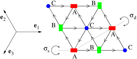
Spin nematic orders have been proposed[24, 25] for the spin-1 triangular lattice material NiGa2S4 which had some experimental evidence of a ground state without magnetic dipole order[26]. In particular Tsunetsugu and Arikawa[24] proposed an interesting three-sublattice spin nematic order, with the directors on the three sublattices perpendicular to each other (see Fig. 1). This state was also found in a numerical study of spin-1 nearest-neighbor bilinear-biquadratic Heisenberg model on triangular lattice[27]. Very recently two groups[28, 29] considered possible spin liquid states by disordering this “Tsunetsugu-Arikawa state” (“antiferroquadrupolar order” in Ref. 27, “tetrad order” in Ref. 29), and found an interesting non-abelian spin liquid with spin-1/2 bosonic spinons coupled to emergent gauge fields in the quaternion group Q8Q_{8}, a discrete non-abelian group with eight elements defined as Q8={±1,±𝕚,±𝕛,±𝕜}Q_{8}=\{\pm 1,\pm\mathbbm{i},\pm\mathbbm{j},\pm\mathbbm{k}\} with the multiplication rule 𝕚2=𝕛2=𝕜2=𝕚​𝕛​𝕜=−1\mathbbm{i}^{2}=\mathbbm{j}^{2}=\mathbbm{k}^{2}=\mathbbm{i}\mathbbm{j}\mathbbm{k}=-1. The continuum field theory for this spin liquid and for the ordering transition, and many interesting properties, e.g. topological degeneracy, have been worked out in Refs. 28, 29. However no microscopic lattice spinon (mean-field) Hamiltonian was given and it was not clear how to construct a spin wavefunction for this “quaternion spin liquid”. The authors of Ref. 28 realized that it is impossible to describe this spin liquid by the Schwinger boson or “bosonic triplon” construction, and suggested that “such a spin liquid cannot be obtained by the standard projective construction for spin liquids”[28]. In this paper a new and non-standard projective construction in terms of a two-orbital Schwinger boson representation of spin-1 will be formulated, and used to construct a mean-field description of the quaternion spin liquid and its ordering transtion to the Tsunetsugu-Arikawa state, and produce a prototype spin wavefunction by projecting the mean-field state.
Refer to caption
Figure 1: (Color online) Triangular lattice with the three sublattices labelled as A,B,CA,B,C respectively. 𝒆1,2,3\boldsymbol{e}_{1,2,3} are three lattice translation vectors. σs\sigma_{s} and σd\sigma_{d} illustrate the two reflection generators of point group C6​vC_{6v}. An example of the three-sublattice spin nematic order[24] is illustrated, with the directors x^,y^,z^\hat{x},\hat{y},\hat{z} drawn as red horizontal bars, green vertical bars, and blue dots, respectively. The quaternion IGG elements on A,B,CA,B,C sites are the A,B,CA,B,C representations of Q8Q_{8} in Eqs. (25a-25c) respectively. Arrow from site rr to r′r^{\prime} means the mean-field ansatz 𝒜r​r′=−𝒜r′​rT=𝒰=(𝟙−i​τx−i​τy+i​τz)/2\mathcal{A}_{rr^{\prime}}=-\mathcal{A}_{r^{\prime}r}^{T}=\mathcal{U}=(\mathbbm{1}-i\tau^{x}-i\tau^{y}+i\tau^{z})/2.

Before proceeding to the new formalism it is worth reviewing how the old Schwinger boson and bosonic triplon constructions fail. The Schwinger boson representation for a spin-SS system[30] is to write the spin operators as (𝝈\boldsymbol{\sigma} are the spin Pauli matrices)

𝑺=12​∑s,s′=↑,↓bs†​𝝈s​s′​bs′,\boldsymbol{S}=\frac{1}{2}\sum_{s,s^{\prime}=\uparrow,\downarrow}b_{s}^{\dagger}\boldsymbol{\sigma}_{ss^{\prime}}^{\vphantom{\dagger}}b_{s^{\prime}}^{\vphantom{\dagger}}, (1)

with the constraint ∑sbs†​bs=2​S\sum_{s}b_{s}^{\dagger}b_{s}^{\vphantom{\dagger}}=2S. This representation has a U⁡(1)U(1) redundancy, b→ei​θ​bb\to e^{i\theta}b (i=−1i=\sqrt{-1}, θ\theta is real). For the gapped spin liquid phase to be stable in two-spatial-dimension(2D) it is necessary to “Higgs” this U⁡(1)U(1) gauge field to a discrete subgroup, usually Z2Z_{2} by boson pairing[20, 21, 31]. However the non-abelian quaternion gauge group is not a subgroup of this abelian U⁡(1)U(1) gauge structure. Moreover it is impossible to describe the spin nematic phase in this formulation as a boson condensate, because a nonzero condensate z=⟨b⟩z=\langle b\rangle necessarily produces a nonzero magnetic dipole moments 𝑴=z†⋅𝝈⋅z/2\boldsymbol{M}=z^{\dagger}\cdot\boldsymbol{\sigma}^{\vphantom{\dagger}}\cdot z^{\vphantom{\dagger}}/2 with size |𝑴|=|z|2/2|\boldsymbol{M}|=|z|^{2}/2.

The bosonic triplon representation[32, 33] uses a three-component boson 𝒃\boldsymbol{b} and writes the spin operator as

𝑺=−i𝒃†×𝒃,\boldsymbol{S}=-i\boldsymbol{b}^{\dagger}\times\boldsymbol{b}^{\vphantom{\dagger}}, (2)

with the constraint 𝒃†⋅𝒃=1\boldsymbol{b}^{\dagger}\cdot\boldsymbol{b}=1. Both magnetic order and spin nematic order can be described by a boson condensate in this construction. However the gauge freedom is again U⁡(1)U(1), 𝒃→ei​θ​𝒃\boldsymbol{b}\to e^{i\theta}\boldsymbol{b}, with no quaternion subgroup. Moreover 𝒃\boldsymbol{b} is not a spin-1/2 representation of spin S​U​(2)SU(2) symmetry. What is needed for the quaternion spin liquid is a new representation of spin-1 by spin-1/2 bosons(like the Schwinger boson) with large enough gauge freedom, which can describe the spin nematic order semiclassically by boson condensation(like the bosonic triplon).

The outline of this paper is as follows. In section I the two-orbital Schwinger boson representation for spin-1 will be introduced. Generic mean-field theories of spin liquids in this representation and related gauge structure and generic (projected) mean-field wavefunctions will be presented. In section II a mean-field Hamiltonian for the quaternion spin liquid on triangular lattice will be constructed and analyzed. The Tsunetsugu-Arikawa state will be obtained by boson condensation. A prototype spin wavefunction for the spin liquid will be presented. In section III remaining issues and possible extensions will be discussed.

I Two-orbital Schwinger Boson Representation of Spin-One and Mean-field Theories for Spin Liquids

Spin-1 can be viewed as a symmetric combination of two spin-1/2. The Affleck-Kennedy-Lieb-Tasaki(AKLT) state was originally defined in this way[34]. Use this “two-orbital” picture and introduce Schwinger bosons for each spin-1/2, the spin-1 operators in terms of the four-component bosons are

𝑺=∑α=12𝑺α=∑α=1212​∑s,s′=↑,↓bα​s†​𝝈s​s′​bα​s′,\boldsymbol{S}=\sum_{\alpha=1}^{2}\boldsymbol{S}_{\alpha}=\sum_{\alpha=1}^{2}\frac{1}{2}\sum_{s,s^{\prime}=\uparrow,\downarrow}b_{\alpha s}^{\dagger}\boldsymbol{\sigma}_{ss^{\prime}}^{\vphantom{\dagger}}b_{\alpha s^{\prime}}^{\vphantom{\dagger}}, (3)

where α=1,2\alpha=1,2 labels orbital, s,s′=↑,↓s,s^{\prime}=\uparrow,\downarrow label spin. This bosonic representation for S​U​(N)SU(N) spins were briefly mentioned in Ref. 35. From this alone the gauge freedom seems to be orbital U⁡(2)U(2), namely bα​s→∑βuα​β​bβ​sb_{\alpha s}\to\sum_{\beta}u_{\alpha\beta}b_{\beta s} with ∑βuα​β∗​uα′​β=δα​α′\sum_{\beta}u_{\alpha\beta}^{*}u_{\alpha^{\prime}\beta}^{\vphantom{\dagger}}=\delta_{\alpha\alpha^{\prime}}^{\vphantom{\dagger}}. However the gauge transformations should also leave the constraints invariant.

The first constraint requires that the total number of bosons is two,

n=∑αnα=∑α​sbα​s†​bα​s=2.n=\sum_{\alpha}n_{\alpha}=\sum_{\alpha s}b^{\dagger}_{\alpha s}b^{\vphantom{\dagger}}_{\alpha s}=2. (4)

Define the orbital pseudo-spins 𝑻\boldsymbol{T} as

𝑻=∑s,α,β12​bα​s†​𝝉α​β​bβ​s,\boldsymbol{T}=\sum_{s,\alpha,\beta}\frac{1}{2}b_{\alpha s}^{\dagger}\boldsymbol{\tau}_{\alpha\beta}^{\vphantom{\dagger}}b_{\beta s}^{\vphantom{\dagger}}, (5)

where 𝝉\boldsymbol{\tau} are orbital Pauli matrices. There are ten states for two bosons, one S=0,T=0S=0,T=0 spin-orbital singlet [2−3/2(b†⋅τyσy⋅b†)|0⟩2^{-3/2}(b^{\dagger}\cdot\tau^{y}\sigma^{y}\cdot b^{\dagger})|0\rangle where |0⟩|0\rangle is the boson vacuum] and nine S=1,T=1S=1,T=1 states. The second constraint is to project out the singlet state,

(b†⋅τy​σy⋅b†)​(b⋅τy​σy⋅b)=0.(b^{\dagger}\cdot\tau^{y}\sigma^{y}\cdot b^{\dagger})(b^{\vphantom{\dagger}}\cdot\tau^{y}\sigma^{y}\cdot b)=0. (6)

The S=1,T=1S=1,T=1 states can be arranged into a matrix, with row and column indices Sz,Tz=1,0,−1S^{z},T^{z}=1,0,-1,

((b1↑†)22b1↑†​b2↑†(b2↑†)22b1↑†​b1↓†b1↑†​b2↓†+b1↓†​b2↑†2b2↑†​b2↓†(b1↓†)22b1↓†​b2↓†(b2↓†)22)⁡|0⟩.\begin{pmatrix}\frac{(b_{1\uparrow}^{\dagger})^{2}}{\sqrt{2}}&b_{1\uparrow}^{\dagger}b_{2\uparrow}^{\dagger}&\frac{(b_{2\uparrow}^{\dagger})^{2}}{\sqrt{2}}\\ b_{1\uparrow}^{\dagger}b_{1\downarrow}^{\dagger}&\frac{b_{1\uparrow}^{\dagger}b_{2\downarrow}^{\dagger}+b_{1\downarrow}^{\dagger}b_{2\uparrow}^{\dagger}}{\sqrt{2}}&b_{2\uparrow}^{\dagger}b_{2\downarrow}^{\dagger}\\ \frac{(b_{1\downarrow}^{\dagger})^{2}}{\sqrt{2}}&b_{1\downarrow}^{\dagger}b_{2\downarrow}^{\dagger}&\frac{(b_{2\downarrow}^{\dagger})^{2}}{\sqrt{2}}\end{pmatrix}|0\rangle. (7)

The physical spin-1 states should be a linear combination of the columns in Eq. (7). This final constraint can be formally represented by

𝓝⋅𝑻=0,\boldsymbol{\mathcal{N}}\cdot\boldsymbol{T}=0, (8)

with complex unit vector 𝓝\boldsymbol{\mathcal{N}} (𝓝∗⋅𝓝=1\boldsymbol{\mathcal{N}}^{*}\cdot\boldsymbol{\mathcal{N}}^{\vphantom{\dagger}}=1). The chosen linear combination has coefficients −(𝒩x−i𝒩y)/2,𝒩z,(𝒩x+i𝒩y)/2-(\mathcal{N}^{x}-i\mathcal{N}^{y})/\sqrt{2},\mathcal{N}^{z},(\mathcal{N}^{x}+i\mathcal{N}^{y})/\sqrt{2} respectively for the three columns in Eq. (7). An equivalent form of Eq. (8) is

∑a,b=x,y,zTa⋅𝒩a∗𝒩b⋅Tb=0.\sum_{a,b=x,y,z}T^{a}\cdot\mathcal{N}^{a*}\mathcal{N}^{b}\cdot T^{b}=0. (9)

The gauge freedom should leave this “vector Higgs condensate” 𝓝\boldsymbol{\mathcal{N}} invariant up to a complex phase, or equivalently leave the hermitian matrix 𝒩a∗𝒩b\mathcal{N}^{a*}\mathcal{N}^{b} invariant.

This parton construction unifies the conventional Schwinger boson Eq. (1) and the two-orbital AKLT representation. For example, 𝓝=(x^+i​y^)/2\boldsymbol{\mathcal{N}}=(\hat{x}+i\hat{y})/\sqrt{2} chooses the first column of Eq. (7) and is the old Schwinger boson representation. In contrast 𝓝=z^\boldsymbol{\mathcal{N}}=\hat{z} chooses the middle column of Eq. (7) and is the AKLT representation. Three different cases of 𝓝\boldsymbol{\mathcal{N}} are discussed in the following.

Case 1): 𝓝∗×𝓝=0\boldsymbol{\mathcal{N}}^{*}\times\boldsymbol{\mathcal{N}}=0, then a complex phase can be chosen so that 𝓝\boldsymbol{\mathcal{N}} is a real vector. This represents an orbital nematic ordered state with the director 𝓝\boldsymbol{\mathcal{N}}, and is equivalent to the AKLT representation. The gauge freedom is U⁡(1)×U⁡(1)⋊Z2U(1)\times U(1)\rtimes Z_{2}, generated by

b→ei​θ​b,b→ei​ϕ​(𝓝⋅𝝉)​b,b→(𝓝⟂⋅𝝉)⋅b,b\to e^{i\theta}b,\quad b\to e^{i\phi(\boldsymbol{\mathcal{N}}\cdot\boldsymbol{\tau})}b,\quad b\to(\boldsymbol{\mathcal{N}}_{\perp}\cdot\boldsymbol{\tau})\cdot b, (10)

where 𝓝⟂\boldsymbol{\mathcal{N}}_{\perp} is a real unit vector perpendicular to 𝓝\boldsymbol{\mathcal{N}}. Note that the last Z2Z_{2} does not commute with the second U⁡(1)U(1) group, therefore semidirect-product ⋊\rtimes is used.

Case 2): 𝓝∗×𝓝≠0\boldsymbol{\mathcal{N}}^{*}\times\boldsymbol{\mathcal{N}}\neq 0 and 𝓝⋅𝓝=0\boldsymbol{\mathcal{N}}\cdot\boldsymbol{\mathcal{N}}=0, then the real and imaginary parts of 𝓝\boldsymbol{\mathcal{N}} are perpendicular to each other and of equal length 1/2\sqrt{1/2}. This represents an orbital dipole ordered state with the orbital moment along 𝑻^=−i𝓝∗×𝓝\hat{\boldsymbol{T}}=-i\boldsymbol{\mathcal{N}}^{*}\times\boldsymbol{\mathcal{N}}, and is equivalent to the single-orbital Schwinger boson representation Eq. (1). The gauge freedom is U⁡(1)U(1),

b→ei​θ​(𝟙+𝑻^⋅𝝉)​b,b\to e^{i\theta(\mathbbm{1}+\hat{\boldsymbol{T}}\cdot\boldsymbol{\tau})}b, (11)

where 𝟙\mathbbm{1} is the identity matrix.

Case 3): 𝓝∗×𝓝≠0\boldsymbol{\mathcal{N}}^{*}\times\boldsymbol{\mathcal{N}}\neq 0 and 𝓝⋅𝓝≠0\boldsymbol{\mathcal{N}}\cdot\boldsymbol{\mathcal{N}}\neq 0, then a complex phase can be chosen so that the real and imaginary parts of 𝓝\boldsymbol{\mathcal{N}} are perpendicular to each other but of different length. The orbital dipole moment is nonzero along 𝑻^=−i𝓝∗×𝓝/|𝓝∗×𝓝|\hat{\boldsymbol{T}}=-i\boldsymbol{\mathcal{N}}^{*}\times\boldsymbol{\mathcal{N}}/|\boldsymbol{\mathcal{N}}^{*}\times\boldsymbol{\mathcal{N}}|. The gauge freedom is U⁡(1)×Z2U(1)\times Z_{2}, generated by

b→ei​θ​b,b→(𝑻^⋅𝝉)⋅b.b\to e^{i\theta}b,\quad b\to(\hat{\boldsymbol{T}}\cdot\boldsymbol{\tau})\cdot b. (12)

Consider the Heisenberg antiferromagnetic interaction between two spin-1 at positions rr and r′r^{\prime}, namely 𝑺r⋅𝑺r′=∑α,β𝑺r​α⋅𝑺r′​β\boldsymbol{S}_{r}\cdot\boldsymbol{S}_{r^{\prime}}=\sum_{\alpha,\beta}\boldsymbol{S}_{r\alpha}\cdot\boldsymbol{S}_{r^{\prime}\beta}. The right-hand-side can be Hubbard-Stratonovich decoupled in the same way as the Schwinger boson mean-field theory[30]. The mean-field Hamiltonian contains spin singlet boson pairing terms, 𝒜r​r′,α​β​(br,α↑†​br′,β↓†−br,α↓†​br′,β↑†)+h.c.\mathcal{A}_{rr^{\prime},\alpha\beta}^{\vphantom{\dagger}}(b_{r,\alpha\uparrow}^{\dagger}b_{r^{\prime},\beta\downarrow}^{\dagger}-b_{r,\alpha\downarrow}^{\dagger}b_{r^{\prime},\beta\uparrow}^{\dagger})+{h.c.}, or in short form br†⋅𝒜r​r′⊗i​σy⋅br′†+h.c.b_{r}^{\dagger}\cdot\mathcal{A}_{rr^{\prime}}^{\vphantom{\dagger}}\otimes i\sigma^{y}\cdot b_{r^{\prime}}^{\dagger}+{h.c.} where 𝒜r​r′\mathcal{A}_{rr^{\prime}} is a generic 2×22\times 2 matrix in the orbital space. Note that 𝒜r′​r=−𝒜r​r′T\mathcal{A}_{r^{\prime}r}^{\vphantom{T}}=-\mathcal{A}_{rr^{\prime}}^{T} where superscript T stands for matrix transpose. For simplicity the boson hopping terms ∑sbr,α​s†​br′,β​s\sum_{s}b^{\dagger}_{r,\alpha s}b^{\vphantom{\dagger}}_{r^{\prime},\beta s} are ignored.

The constraints must be included in the mean-field theory by introducing onsite terms with Langrange multipliers[36]. The first constraint Eq. (4) can be incorporated by a chemical potential μ\mu as μ⁡(n−2)\mu(n-2). The second one Eq. (6) may be included as −λ⁡(b†⋅τy​σy⋅b†)​(b⋅τy​σy⋅b)-\lambda(b^{\dagger}\cdot\tau^{y}\sigma^{y}\cdot b^{\dagger})(b^{\vphantom{\dagger}}\cdot\tau^{y}\sigma^{y}\cdot b) with real λ\lambda, however this is not quadratic in terms of bosons. A non-rigorous Hubbard-Stratonovich decoupling can be performed to reduce this term to −η⁡(b†⋅τy​σy⋅b†)−η∗​(b⋅τy​σy⋅b)+|η|2/λ-\eta(b^{\dagger}\cdot\tau^{y}\sigma^{y}\cdot b^{\dagger})-\eta^{*}(b^{\vphantom{\dagger}}\cdot\tau^{y}\sigma^{y}\cdot b)+|\eta|^{2}/\lambda with a complex Langrange multiplier η\eta. This procedure may be made rigorous regardless of the sign of λ\lambda by the tricks of Ref. 37. The final constraint Eq. (8) may be included as −μ′𝓝⋅𝑻+h.c.-\mu^{\prime}\boldsymbol{\mathcal{N}}\cdot\boldsymbol{T}+{h.c.} with a complex Lagrange multiplier μ′\mu^{\prime}. In summary the generic mean-field Hamiltonian for spin liquids is

HMF=−∑r,r′[br†⋅𝒜r​r′⊗iσy⋅br′†+h.c.]+∑rμrnr−∑r[ηr(b†r⋅τyσy⋅b†r)+h.c.]−∑r[br†⋅ℜ(μ′r𝓝r)⋅𝝉⋅br]+const.,\begin{split}H_{\rm MF}=\ &-\sum_{r,r^{\prime}}[b_{r}^{\dagger}\cdot\mathcal{A}_{rr^{\prime}}^{\vphantom{\dagger}}\otimes i\sigma^{y}\cdot b_{r^{\prime}}^{\dagger}+{h.c.}]+\sum_{r}\mu_{r}^{\vphantom{\dagger}}n_{r}^{\vphantom{\dagger}}\\ &-\sum_{r}[\eta_{r}(b^{\dagger}_{r}\cdot\tau^{y}\sigma^{y}\cdot b^{\dagger}_{r})+{h.c.}]\\ &-\sum_{r}[b_{r}^{\dagger}\cdot\Re(\mu^{\prime}_{r}\boldsymbol{\mathcal{N}}_{r})\cdot\boldsymbol{\tau}\cdot b_{r}^{\vphantom{\dagger}}]+{const.},\end{split} (13)

where ℜ\Re means real part. The mean-field constraints are

⟨nr⟩MF=2,⟨b†r⋅τyσy⋅b†r⟩MF=0,⟨br†⋅(𝓝r⋅𝝉)⋅br⟩MF=0.\begin{split}&\langle n_{r}\rangle_{\rm MF}=2,\quad\langle b^{\dagger}_{r}\cdot\tau^{y}\sigma^{y}\cdot b^{\dagger}_{r}\rangle_{\rm MF}=0,\quad\\ &\langle b_{r}^{\dagger}\cdot(\boldsymbol{\mathcal{N}}_{r}\cdot\boldsymbol{\tau})\cdot b_{r}^{\vphantom{\dagger}}\rangle_{\rm MF}=0.\end{split} (14)

The mean-field Hamiltonian Eq. (13) is not gauge invariant. Under a site-dependent gauge transformation br→G⁡(r)⋅brb_{r}\to G(r)\cdot b_{r}, the mean-field ansatz {μr,ηr,μr′,𝓝r,𝒜r​r′}\{\mu_{r},\eta_{r},\mu^{\prime}_{r},\boldsymbol{\mathcal{N}}_{r},\mathcal{A}_{rr^{\prime}}\} should transform as

𝒜r​r′→G(r)⋅𝒜r​r′⋅GT(r′),ηr→e2​i​θηr,μr+ℜ⁡(μr′​𝓝r)⋅𝝉→G⁡(r)⋅[μr+ℜ⁡(μr′​𝓝r)⋅𝝉]⋅G−1​(r),\begin{split}&\mathcal{A}_{rr^{\prime}}\to G(r)\cdot\mathcal{A}_{rr^{\prime}}\cdot G^{T}(r^{\prime}),\quad\eta_{r}\to e^{2i\theta}\eta_{r},\\ &\mu_{r}+\Re(\mu^{\prime}_{r}\boldsymbol{\mathcal{N}}_{r})\cdot\boldsymbol{\tau}\to G(r)\cdot[\mu_{r}+\Re(\mu^{\prime}_{r}\boldsymbol{\mathcal{N}}_{r})\cdot\boldsymbol{\tau}]\cdot G^{-1}(r),\end{split} (15)

where θ\theta defines the orbital-independent U⁡(1)U(1) subgroup in Eqs. (10-12). Gauge-invariant fluxes can be defined in analogy to the Schwinger boson or S​p​(N)Sp(N) boson theory[38]. The loop expansion for the mean-field ground state energy can also be performed, and a “flux expulsion” argument for Heisenberg models may be raised as well[38].

A realistic spin-1 Hamiltonian may contain the biquadratic interactions (𝑺r⋅𝑺r′)2(\boldsymbol{S}_{r}\cdot\boldsymbol{S}_{r^{\prime}})^{2} and multiple-spin interactions, which cannot be simply decoupled into quadratic terms of bosons. In this situation it is better to view the mean-field theory as a variational approach. The mean-field ground state after projection to physical spin-1 space can be used as a variational wavefunction. This viewpoint will be adopted throughout this paper, so no self-consistent equation of 𝒜\mathcal{A} will be solved, and the overall scale of the ansatz does not matter.

The mean-field ground state |MF⟩|{\rm MF}\rangle is generically

|MF⟩=exp⁡[12​∑r,r′br†⋅fr​r′⊗i​σy⋅br′†]​|0⟩,|{\rm MF}\rangle=\exp\Big[\frac{1}{2}\sum_{r,r^{\prime}}b^{\dagger}_{r}\cdot f_{rr^{\prime}}^{\vphantom{\dagger}}\otimes i\sigma^{y}\cdot b^{\dagger}_{r^{\prime}}\Big]\big|0\big\rangle, (16)

where fr​r′f_{rr^{\prime}} are 2×22\times 2 matrices in the orbital space, and have the same symmetry and gauge transformation rule as the mean-field ansatz 𝒜r​r′\mathcal{A}_{rr^{\prime}}, e.g. fr′​r=−fr​r′Tf_{r^{\prime}r}^{\vphantom{\dagger}}=-f_{rr^{\prime}}^{T}. r=r′r=r^{\prime} term with fr​r=−fr​rT∝τyf_{rr}^{\vphantom{\dagger}}=-f_{rr}^{T}\propto\tau^{y} is allowed but creates only onsite spin singlet and will be projected out. Each fr​r′,α​β​(bα↑†​bβ↓†−bα↓†​bβ↑†)f_{rr^{\prime},\alpha\beta}^{\vphantom{\dagger}}(b^{\dagger}_{\alpha\uparrow}b^{\dagger}_{\beta\downarrow}-b^{\dagger}_{\alpha\downarrow}b^{\dagger}_{\beta\uparrow}) term creates a spin singlet from two spin-1/2 on bond r​r′rr^{\prime}. The projection onto physical spin-1 space requires two bosons on every site and the onsite symmetrization of the two orbitals. The projected wave function 𝒫​|MF⟩\mathcal{P}|{\rm MF}\rangle is therefore a superposition of close-packed (every site is covered once) loop configurations {ℓ}\{\ell\}, and on each loop ℓ\ell the spin-1 form an AKLT state,

𝒫⁡|MF⟩=∑{ℓ}∏ℓWℓ​|AKLT​on​ℓ⟩.\mathcal{P}|{\rm MF}\rangle=\sum_{\{\ell\}}\prod_{\ell}W_{\ell}|{\rm AKLT\ on\ }\ell\rangle. (17)

The “close-packed” loop configurations may involve bonds longer than nearest-neighbor. The amplitude factor WℓW_{\ell} for a length-LL loop ℓ=(r1​r2​…​rL)\ell=(r_{1}r_{2}\dots r_{L}) is

Wℓ=(3/4)L/2⋅NL⋅Tr⁡[τr1​fr1​r2​τr2​fr2​r3​…​τrL​frL​r1],\begin{split}W_{\ell}=\ &(3/4)^{L/2}\cdot N_{L}\cdot\mathrm{Tr}[\tau_{r_{1}}f_{r_{1}r_{2}}\tau_{r_{2}}f_{r_{2}r_{3}}\dots\tau_{r_{L}}f_{r_{L}r_{1}}],\end{split} (18)

where Tr\mathrm{Tr} means matrix trace, NL=1+3⋅(−3)−LN_{L}=\sqrt{1+3\cdot(-3)^{-L}}, and τr=−iτy⋅(𝓝r∗⋅𝝉)\tau_{r}=-i\tau^{y}\cdot(\boldsymbol{\mathcal{N}}_{r}^{*}\cdot\boldsymbol{\tau}) comes from the contraint Eq. (8) (τr=τx\tau_{r}=\tau^{x} when 𝓝r=z^\boldsymbol{\mathcal{N}}_{r}=\hat{z}). The factor (3/4)L/2⋅NL(3/4)^{L/2}\cdot N_{L} is the overlap between one spin-1/2 dimer pattern and the AKLT state[34]. (3/4)L/2(3/4)^{L/2} produces an overall factor for the wavefunction and can be omitted. NL∼1N_{L}\sim 1 when LL is large. WℓW_{\ell} is gauge invariant up to a global factor, due to the fact that GT​(r)⋅(−i​τy)⋅(𝓝r∗⋅𝝉)⋅G⁡(r)=e2​i​θ​(−i​τy)⋅G−1​(r)⋅(𝓝r∗⋅𝝉)⋅G⁡(r)∼(−i​τy)⋅(𝓝r∗⋅𝝉)G^{T}(r)\cdot(-i\tau^{y})\cdot(\boldsymbol{\mathcal{N}}_{r}^{*}\cdot\boldsymbol{\tau})\cdot G(r)=e^{2i\theta}(-i\tau^{y})\cdot G^{-1}(r)\cdot(\boldsymbol{\mathcal{N}}_{r}^{*}\cdot\boldsymbol{\tau})\cdot G(r)\sim(-i\tau^{y})\cdot(\boldsymbol{\mathcal{N}}_{r}^{*}\cdot\boldsymbol{\tau}) up to a complex phase, for any G⁡(r)G(r) in the gauge group Eqs. (10-12). LL can be 22 in which case the AKLT state is the “double-bond” spin singlet state formed by two spin-1.

Wavefunctions for spin-1/2 spinon and gauge flux excitations can be constructed as well. The mean-field state with two spinons at r,r′r,r^{\prime} is given by

|ℬr,ℬr′⟩MF=Tr[ℬ^r†⋅ℬr]Tr[ℬ^r′†⋅ℬr′]|MF⟩|\mathcal{B}_{r\vphantom{r^{\prime}}}^{\vphantom{\dagger}},\mathcal{B}_{r^{\prime}}^{\vphantom{\dagger}}\rangle_{\rm MF}=\mathrm{Tr}[\hat{\mathcal{B}}_{r\vphantom{r^{\prime}}}^{\dagger}\cdot\mathcal{B}_{r\vphantom{r^{\prime}}}^{\vphantom{\dagger}}]\mathrm{Tr}[\hat{\mathcal{B}}_{r^{\prime}}^{\dagger}\cdot\mathcal{B}_{r^{\prime}}^{\vphantom{\dagger}}]|{\rm MF}\rangle (19)

where ℬr,r′\mathcal{B}_{r,r^{\prime}} are 2×22\times 2 complex spinon state matrices, and

ℬ^=(b1↑b2↑b1↓b2↓).\hat{\mathcal{B}}=\begin{pmatrix}b_{1\uparrow}&b_{2\uparrow}\\ b_{1\downarrow}&b_{2\downarrow}\end{pmatrix}. (20)

Projecting this state onto spin-1 space creates a superposition of configurations with one open AKLT chain ℓr​r′\ell_{rr^{\prime}} from rr to r′r^{\prime} plus close-packed AKLT loops. The direction of the end-spins of open AKLT chain are given by Tr⁡[ℬ†​𝝈​ℬ]\mathrm{Tr}[\mathcal{B}^{\dagger}\boldsymbol{\sigma}\mathcal{B}] (normalization requires |Tr⁡[ℬ†​𝝈​ℬ]|=1|\mathrm{Tr}[\mathcal{B}^{\dagger}\boldsymbol{\sigma}\mathcal{B}]|=1). The amplitude for a length-(L+2)(L+2) open chain ℓr​r′=(r​r1​…​rL​r′)\ell_{rr^{\prime}}=(rr_{1}\dots r_{L}r^{\prime}) with the end-spins at r,r′r,r^{\prime} in SzS^{z} eigenstates s,s′=↑,↓s,s^{\prime}=\uparrow,\downarrow is (LL can be zero)

Wℓr​r′,s​s′=(3/4)L/2+1⋅NL,s​s′×(ℬr​τr​fr​r1​τr1​fr1​r2​…​τrL​frL​r′​τr′​ℬr′T)s​s′,\begin{split}W_{\ell_{rr^{\prime}},ss^{\prime}}=\ &(3/4)^{L/2+1}\cdot N_{L,ss^{\prime}}\\ &\times(\mathcal{B}_{r}^{\vphantom{\dagger}}\tau_{r}f_{rr_{1}}^{\vphantom{\dagger}}\tau_{r_{1}}f_{r_{1}r_{2}}^{\vphantom{\dagger}}\dots\tau_{r_{L}}f_{r_{L}r^{\prime}}^{\vphantom{\dagger}}\tau_{r^{\prime}}\mathcal{B}_{r^{\prime}}^{T})_{ss^{\prime}}^{\vphantom{\dagger}},\end{split} (21)

with[34] NL,s​s′=1+(−3)−L−2​(σx−𝟙)s​s′N_{L,ss^{\prime}}=\sqrt{1+(-3)^{-L-2}(\sigma^{x}-\mathbbm{1})_{ss^{\prime}}}. Multiple (even) number of spinons can be constructed similarly. Gauge flux excitations and topological degeneracy of ground states will be demonstrated in the quantum limit of quaternion spin liquid in subsection II.3.

Spin liquids described in this way will have gapped spin-1/2 bosonic spinons. For them to be stable in 2D it is necessary to “Higgs” the continuous compact gauge groups Eqs. (10-12) to a discrete subgroup. Many possibilities exist which can in principle be completely classified by the projective symmetry group(PSG) method[39, 36, 40, 41]. This brute-force approach will not be attempted here, but the PSG language will be used to show that the mean-field theory indeed describes a spin liquid state with no symmetry breaking. This will be achieved by the explicit construction of the PSG elements, br→GX​(r)⋅bX⁡(r)b_{r}\to G_{X}(r)\cdot b_{X(r)}, for all generators XX of the physical symmetry group (space group and time-reversal). The mean-field Hamiltonian shall be invariant under PSG actions.

The case with uniform 𝓝r=z^\boldsymbol{\mathcal{N}}_{r}=\hat{z} will be considered hereafter only, except subsection II.4. The physical spin-1 states |Sz=+1,0,−1⟩|S^{z}=+1,0,-1\rangle are

|Sz=+1⟩\displaystyle|S^{z}=+1\rangle =\displaystyle= b1↑†​b2↑†​|0⟩,\displaystyle b_{1\uparrow}^{\dagger}b_{2\uparrow}^{\dagger}|0\rangle, (22a)
|Sz=0⟩\displaystyle|S^{z}=0\rangle =\displaystyle= 12​(b1↑†​b2↓†+b1↓†​b2↑†)​|0⟩,\displaystyle\frac{1}{\sqrt{2}}(b_{1\uparrow}^{\dagger}b_{2\downarrow}^{\dagger}+b_{1\downarrow}^{\dagger}b_{2\uparrow}^{\dagger})|0\rangle, (22b)
|Sz=−1⟩\displaystyle|S^{z}=-1\rangle =\displaystyle= b1↓†​b2↓†​|0⟩.\displaystyle b_{1\downarrow}^{\dagger}b_{2\downarrow}^{\dagger}|0\rangle. (22c)

The constraints Eq. (4) and Eq. (8) can be rewritten as

nα=∑sb†α​sbα​s=1,α=1,2.n_{\alpha}=\sum_{s}b^{\dagger}_{\alpha s}b^{\vphantom{\dagger}}_{\alpha s}=1,\quad\alpha=1,2. (23)

The U⁡(1)×U⁡(1)⋊Z2U(1)\times U(1)\rtimes Z_{2} gauge group is,

b→ei​θ​(cos⁡ϕ⋅𝟙+sin⁡ϕ⋅i​τz)⋅b,orb→ei​θ​(cos⁡ϕ⋅i​τx+sin⁡ϕ⋅i​τy)⋅b.\begin{split}&b\to e^{i\theta}(\cos\phi\cdot\mathbbm{1}+\sin\phi\cdot i\tau^{z})\cdot b,\quad{\rm or\ }\\ &b\to e^{i\theta}(\cos\phi\cdot i\tau^{x}+\sin\phi\cdot i\tau^{y})\cdot b.\end{split} (24)

For frustrated(e.g. triangular) lattices the orbital-independent U⁡(1)U(1) freedom ei​θe^{i\theta} will be removed by boson pairings in mean-field theory. The remaining U⁡(1)⋊Z2U(1)\rtimes Z_{2} [a subgroup of S​U​(2)SU(2) by setting θ=0\theta=0 in Eq. (24)] will be the starting point of discussions hereafter. It is non-abelian and contains the quaternion group.

A semiclassical picture of the uniaxial spin nematic order is that the two spin-1/2 have dipole moments antiparallel to each other and along the direction of the director, ⟨𝑺1⟩=−⟨𝑺2⟩∝𝒏\langle\boldsymbol{S}_{1}\rangle=-\langle\boldsymbol{S}_{2}\rangle\propto\boldsymbol{n}. This can be achieved by a single spin-orbital-entangled condensate, e.g. ⟨(b1↑,b1↓,b2↑,b2↓)⟩∝(1,0,0,1)\langle(b_{1\uparrow},b_{1\downarrow},b_{2\uparrow},b_{2\downarrow})\rangle\propto(1,0,0,1) for 𝒏∝z^\boldsymbol{n}\propto\hat{z}. However the quadrupole order parameter Qa​bQ^{ab} is naively zero because ⟨Sa⟩\langle S^{a}\rangle is zero. This can be remedied by recognizing that Qa​b=⟨∑α,β(Sαa​Sβb+Sαb​Sβa)⟩/2−(2/3)​δa​b=⟨S1a​S2b+S1b​S2a⟩−(1/6)​δa​bQ^{ab}=\langle\sum_{\alpha,\beta}(S^{a}_{\alpha}S^{b}_{\beta}+S^{b}_{\alpha}S^{a}_{\beta})\rangle/2-(2/3)\delta^{ab}=\langle S^{a}_{1}S^{b}_{2}+S^{b}_{1}S^{a}_{2}\rangle-(1/6)\delta^{ab}, and the last expression is nontrivial in this condensate state [although not in the form of na​nb−(1/3)​δa​b​𝒏2n^{a}n^{b}-(1/3)\delta^{ab}\boldsymbol{n}^{2}]. This can be further justified by projecting the coherent state from this condensate exp⁡[w⁡(b1↑†+b2↓†)]​|0⟩\exp[w\,(b_{1\uparrow}^{\dagger}+b_{2\downarrow}^{\dagger})]|0\rangle onto the physical spin-1 states Eqs. (22a-22c), which gives the uniaxial spin nematic state (w2/2)|Sz=0⟩(w^{2}/\sqrt{2})|S^{z}=0\rangle with director along z^\hat{z} direction. In general the nematic director from a condensate ⟨b⟩\langle b\rangle is given by ⟨b⟩∗⋅τz​𝝈⋅⟨b⟩\langle b\rangle^{*}\cdot\tau^{z}\boldsymbol{\sigma}\cdot\langle b\rangle.

II Quaternion Spin Liquid on Triangular Lattice

For a mean-field theory of quaternion spin liquid, the invariant gauge group(IGG)[39, 36] must be a representation of the quaternion group Q8={±1,±𝕚,±𝕛,±𝕜}Q_{8}=\{\pm 1,\pm\mathbbm{i},\pm\mathbbm{j},\pm\mathbbm{k}\}, with eight distinct IGG elements Gq​(r)∈U⁡(1)⋊Z2G_{q}(r)\in U(1)\rtimes Z_{2} such that: 1) the ansatz {μr,ηr,μr′,𝓝r=z^,𝒜r​r′}\{\mu_{r},\eta_{r},\mu^{\prime}_{r},\boldsymbol{\mathcal{N}}_{r}=\hat{z},\mathcal{A}_{rr^{\prime}}\} are invariant under the actions Eq. (15) of Gq​(r)G_{q}(r) for any q∈Q8q\in Q_{8}, and no other element of Eq. (24) can do the same; 2) Gq​(r)G_{q}(r) is a representation of Q8Q_{8} for any site rr.

There are three distinct classes (labelled by A,B,CA,B,C) of Q8Q_{8} representations on a single site. Representatives of each class are given below (G±1=±𝟙G_{\pm 1}=\pm\mathbbm{1} for all classes),

A:\displaystyle A: G±𝕚=∓i​τx,G±𝕛=∓i​τy,G±𝕜=∓i​τz;\displaystyle G_{\pm\mathbbm{i}}=\mp i\tau^{x},\ G_{\pm\mathbbm{j}}=\mp i\tau^{y},\ G_{\pm\mathbbm{k}}=\mp i\tau^{z}; (25a)
B:\displaystyle B: G±𝕚=∓i​τy,G±𝕛=∓i​τz,G±𝕜=∓i​τx;\displaystyle G_{\pm\mathbbm{i}}=\mp i\tau^{y},\ G_{\pm\mathbbm{j}}=\mp i\tau^{z},\ G_{\pm\mathbbm{k}}=\mp i\tau^{x}; (25b)
C:\displaystyle C: G±𝕚=∓i​τz,G±𝕛=∓i​τx,G±𝕜=∓i​τy.\displaystyle G_{\pm\mathbbm{i}}=\mp i\tau^{z},\ G_{\pm\mathbbm{j}}=\mp i\tau^{x},\ G_{\pm\mathbbm{k}}=\mp i\tau^{y}. (25c)

Each class is generated by group conjugacy on its representative, Gq→G⋅Gq⋅G−1G_{q}\to G\cdot G_{q}\cdot G^{-1} for G∈U⁡(1)⋊Z2G\in U(1)\rtimes Z_{2}. Therefore by site(rr)-dependent gauge transformations all Gq​(r)G_{q}(r) can be reduced to one of those in Eqs. (25a-25c).

These Q8Q_{8} IGGs will constrain allowed ansatzs. For the onsite terms, the Q8Q_{8} IGGs demand μr′=0\mu^{\prime}_{r}=0 but put no constraint on ηr\eta_{r}. On the converse, however, μr′=0\mu^{\prime}_{r}=0 and ηr\eta_{r} do not reduce the U⁡(1)⋊Z2U(1)\rtimes Z_{2} freedom.

Consider a bond r​r′rr^{\prime} with nonzero 𝒜r​r′\mathcal{A}_{rr^{\prime}}. The Q8Q_{8} IGGs demand 𝒜r​r′=Gq​(r)⋅𝒜r​r′⋅Gq​(r′)T\mathcal{A}_{rr^{\prime}}=G_{q}(r)\cdot\mathcal{A}_{rr^{\prime}}\cdot G_{q}(r^{\prime})^{T} for all q∈Q8q\in Q_{8}. There are three possibilities for 𝒜r​r′\mathcal{A}_{rr^{\prime}} depending on the representation choice combinations (r​r′)(rr^{\prime}),

𝒜r​r′∝{τy,(r​r′)=(A​A),(B​B),(C​C),𝒰,(r​r′)=(A​B),(B​C),(C​A),𝒰T,(r​r′)=(A​C),(B​A),(C​B),\mathcal{A}_{rr^{\prime}}\propto\left\{\begin{array}[]{ll}\tau^{y},&(rr^{\prime})=(AA),(BB),(CC),\\ \mathcal{U},&(rr^{\prime})=(AB),(BC),(CA),\\ \mathcal{U}^{T},&(rr^{\prime})=(AC),(BA),(CB),\end{array}\right. (26)

where the S​U​(2)SU(2) matrix 𝒰=(𝟙−i​τx−i​τy+i​τz)/2\mathcal{U}=(\mathbbm{1}-i\tau^{x}-i\tau^{y}+i\tau^{z})/2 will appear frequently. Consider the converse problem, namely whether 𝒜r​r′\mathcal{A}_{rr^{\prime}} can “Higgs” the gauge freedom to Q8Q_{8}. 𝒜r​r′∝τy\mathcal{A}_{rr^{\prime}}\propto\tau^{y} will not do this job, because all G⁡(r)=G⁡(r′)∈U⁡(1)⋊Z2G(r)=G(r^{\prime})\in U(1)\rtimes Z_{2} will keep 𝒜r​r′∝τy\mathcal{A}_{rr^{\prime}}\propto\tau^{y} invariant. The other two possibilities 𝒜r​r′=𝒰\mathcal{A}_{rr^{\prime}}=\mathcal{U} or 𝒰T\mathcal{U}^{T} will reduce the gauge freedom to Q8Q_{8} with the representation choices given above. For instance consider G⁡(r′)=cos⁡ϕ⋅𝟙+sin⁡ϕ⋅i​τzG(r^{\prime})=\cos\phi\cdot\mathbbm{1}+\sin\phi\cdot i\tau^{z} and 𝒜r​r′=𝒰\mathcal{A}_{rr^{\prime}}=\mathcal{U}, the constraint solves for G⁡(r)=cos⁡ϕ⋅𝟙+sin⁡ϕ⋅i​τyG(r)=\cos\phi\cdot\mathbbm{1}+\sin\phi\cdot i\tau^{y} which can be a member of the U⁡(1)⋊Z2U(1)\rtimes Z_{2} group only if ϕ\phi is a integral multiple of π/2\pi/2, restricting G⁡(r)G(r) and G⁡(r′)G(r^{\prime}) to be members of Q8Q_{8} representations.

II.1 Mean-field Theory on Triangular Lattice

With the above general considerations a mean-field Hamiltonian of quaternion spin liquid can be constructed on the triangular lattice. Due to the three-sublattice structure it is natural to assign the three Q8Q_{8} representations to the three corresponding sublattices. In this paper only the nearest-neighbor ansatz will be considered, with 𝒜r​r′=𝒰\mathcal{A}_{rr^{\prime}}=\mathcal{U} or −𝒰T-\mathcal{U}^{T} as shown in Fig. 1. Note that by the variational interpretation the overall scale of 𝒜r​r′\mathcal{A}_{rr^{\prime}} does not matter, and the overall complex phase of 𝒜r​r′\mathcal{A}_{rr^{\prime}} can be removed by a global orbital-independent U⁡(1)U(1) phase rotation of bosons. Translation symmetry further requires uniform μr=μ\mu_{r}=\mu and ηr=η\eta_{r}=\eta.

The mean-field Hamiltonian reads (up to a constant),

HMF=∑𝒓[μn𝒓−(ηb†𝒓⋅τyσy⋅b†𝒓+h.c.)−∑d=13(b†𝒓⋅𝒰⊗iσy⋅b†𝒓+𝒆d+h.c.)].\begin{split}H_{\rm MF}=\ &\sum_{\boldsymbol{r}}\Big[\mu\,n_{\boldsymbol{r}}-(\eta\,b^{\dagger}_{\boldsymbol{r}}\cdot\tau^{y}\sigma^{y}\cdot b^{\dagger}_{\boldsymbol{r}}+h.c.)\\ &\phantom{\sum_{\boldsymbol{r}}\Big[}-\sum_{d=1}^{3}(b^{\dagger}_{\boldsymbol{r}}\cdot\mathcal{U}\otimes i\sigma^{y}\cdot b^{\dagger}_{\boldsymbol{r}+\boldsymbol{e}_{d}}+{h.c.})\Big].\end{split} (27)

Physical symmetries are generated by two translations T1,2T_{1,2} along 𝒆1,2\boldsymbol{e}_{1,2}, two reflections σs\sigma_{s} and σd\sigma_{d} (see Fig. 1), and time-reversal 𝒯\mathcal{T}. T1,2T_{1,2} and σs\sigma_{s} are trivial. σd\sigma_{d} reverses all bond orientations in Fig. 1. 𝒯\mathcal{T} changes the ansatz to their complex conjugate. Corresponding PSG elements are,

T1,2\displaystyle T_{1,2} :\displaystyle: b𝒓→b𝒓+𝒆1,2,\displaystyle b_{\boldsymbol{r}}\to b_{\boldsymbol{r}+\boldsymbol{e}_{1,2}}, (28a)
σs\displaystyle\sigma_{s} :\displaystyle: b𝒓→bσs​(𝒓),\displaystyle b_{\boldsymbol{r}}\to b_{\sigma_{s}(\boldsymbol{r})}, (28b)
σd\displaystyle\sigma_{d} :\displaystyle: b𝒓→1/2​(i​τx−i​τy)⋅bσd​(𝒓),\displaystyle b_{\boldsymbol{r}}\to\sqrt{1/2}(i\tau^{x}-i\tau^{y})\cdot b_{\sigma_{d}(\boldsymbol{r})}, (28c)
𝒯\displaystyle\mathcal{T} :\displaystyle: b𝒓→τy​σy⋅b𝒓.\displaystyle b_{\boldsymbol{r}}\to\tau^{y}\sigma^{y}\cdot b_{\boldsymbol{r}}. (28d)

The Q8Q_{8} IGG is defined in Eqs. (25a-25c) for A,B,CA,B,C sublattices respectively. Time-reversal symmetry restricts η\eta to be real. With this PSG constructed the mean-field Hamiltonian describes a “symmetric spin liquid”[36] with no broken symmetry.

The mean-field Hamiltonian can be solved in the same way as the Schwinger boson mean-field theories[31]. Do the Fourier transform b𝒌=Nsite−1/2∑𝒓e−i𝒌⋅𝒓b𝒓b_{\boldsymbol{k}}=N_{\rm site}^{-1/2}\sum_{\boldsymbol{r}}e^{-i\boldsymbol{k}\cdot\boldsymbol{r}}b_{\boldsymbol{r}} where NsiteN_{\rm site} is the number of sites, and define Ψ𝒌=(b𝒌,1↑,b𝒌,2↑,b−𝒌,1↓†,b−𝒌,2↓†)T\Psi_{\boldsymbol{k}}=(b_{\boldsymbol{k},1\uparrow}^{\vphantom{\dagger}},b_{\boldsymbol{k},2\uparrow}^{\vphantom{\dagger}},b_{-\boldsymbol{k},1\downarrow}^{\dagger},b_{-\boldsymbol{k},2\downarrow}^{\dagger})^{T}, Eq. (27) becomes

HMF=∑𝒌[Ψ𝒌†⋅(μ​ 1−P𝒌−P𝒌†μ​ 1)⋅Ψ𝒌−2​μ].H_{\rm MF}=\sum_{\boldsymbol{k}}\Big[\Psi_{\boldsymbol{k}}^{\dagger}\cdot\begin{pmatrix}\mu\,\mathbbm{1}&-P_{\boldsymbol{k}}\\ -P_{\boldsymbol{k}}^{\dagger}&\mu\,\mathbbm{1}\end{pmatrix}\cdot\Psi_{\boldsymbol{k}}^{\vphantom{\dagger}}-2\mu\Big]. (29)

where P𝒌=i⁡(𝟙−i​τx+i​τz)​ℑ⁡ξ𝒌−i​τy​(ℜ⁡ξ𝒌+η)P_{\boldsymbol{k}}=i(\mathbbm{1}-i\tau^{x}+i\tau^{z})\,\Im\xi_{\boldsymbol{k}}-i\tau^{y}(\Re\xi_{\boldsymbol{k}}+\eta), ℜ\Re and ℑ\Im are real and imaginary parts, ξ𝒌=ei​𝒌⋅𝒆1+ei​𝒌⋅𝒆2+ei​𝒌⋅𝒆3\xi_{\boldsymbol{k}}=e^{i\boldsymbol{k}\cdot\boldsymbol{e}_{1}}+e^{i\boldsymbol{k}\cdot\boldsymbol{e}_{2}}+e^{i\boldsymbol{k}\cdot\boldsymbol{e}_{3}}. Do a singular value decomposition

P𝒌=U𝒌⋅(ρ1​(𝒌)00ρ2​(𝒌))⋅V𝒌†P_{\boldsymbol{k}}=U_{\boldsymbol{k}}^{\vphantom{\dagger}}\cdot\begin{pmatrix}\rho_{1}(\boldsymbol{k})&0\\ 0&\rho_{2}(\boldsymbol{k})\end{pmatrix}\cdot V_{\boldsymbol{k}}^{\dagger} (30)

with U⁡(2)U(2) matrices U𝒌,V𝒌U_{\boldsymbol{k}},V_{\boldsymbol{k}} given by

U𝒌\displaystyle U_{\boldsymbol{k}} =\displaystyle= (−13+313−3ei​π/4​13−3ei​π/4​13+3),\displaystyle\begin{pmatrix}-\sqrt{\frac{1}{3+\sqrt{3}}}&\sqrt{\frac{1}{3-\sqrt{3}}}\\ e^{i\pi/4}\sqrt{\frac{1}{3-\sqrt{3}}}&e^{i\pi/4}\sqrt{\frac{1}{3+\sqrt{3}}}\end{pmatrix}, (31)
V𝒌\displaystyle V_{\boldsymbol{k}} =\displaystyle= (ei​π/4​13−3−ei​π/4​13+313+313−3),\displaystyle\begin{pmatrix}e^{i\pi/4}\sqrt{\frac{1}{3-\sqrt{3}}}&-e^{i\pi/4}\sqrt{\frac{1}{3+\sqrt{3}}}\\ \sqrt{\frac{1}{3+\sqrt{3}}}&\sqrt{\frac{1}{3-\sqrt{3}}}\end{pmatrix}, (32)

and real singular values ρ1,2​(𝒌)=3​ℑ⁡ξ𝒌±(ℜ⁡ξ𝒌+η).\rho_{1,2}(\boldsymbol{k})=\sqrt{3}\,\Im\xi_{\boldsymbol{k}}\pm(\Re\xi_{\boldsymbol{k}}+\eta). Define “Bogoliubov quasiparticles”

Φ𝒌=(γ𝒌,1↑γ𝒌,2↑γ−𝒌,1↓†γ−𝒌,2↓†)=(C10S100C20S2S10C100S20C2)​(U𝒌†02×202×2V𝒌†)​Ψ𝒌,\Phi_{\boldsymbol{k}}=\begin{pmatrix}\gamma_{\boldsymbol{k},1\uparrow}\\ \gamma_{\boldsymbol{k},2\uparrow}\\ \gamma_{-\boldsymbol{k},1\downarrow}^{\dagger}\\ \gamma_{-\boldsymbol{k},2\downarrow}^{\dagger}\end{pmatrix}=\begin{pmatrix}C_{1}&0&S_{1}&0\\ 0&C_{2}&0&S_{2}\\ S_{1}&0&C_{1}&0\\ 0&S_{2}&0&C_{2}\end{pmatrix}\begin{pmatrix}U_{\boldsymbol{k}}^{\dagger}&0_{2\times 2}\\ 0_{2\times 2}&V_{\boldsymbol{k}}^{\dagger}\end{pmatrix}\Psi_{\boldsymbol{k}}, (33)

where C1,2=1+μ/E1,2​(𝒌)/2C_{1,2}=\sqrt{1+\mu/E_{1,2}(\boldsymbol{k})}/\sqrt{2} and S1,2=−ρ1,2(𝒌)/E1,2(𝒌)/2C1,2S_{1,2}=-\rho_{1,2}(\boldsymbol{k})/E_{1,2}(\boldsymbol{k})/2C_{1,2}, with the mean-field dispersions

E1,2​(𝒌)=μ2−ρ1,22​(𝒌).E_{1,2}(\boldsymbol{k})=\sqrt{\mu^{2}-\rho_{1,2}^{2}(\boldsymbol{k})}. (34)

Eq. (29) is diagonalized by this S​U​(2,2)SU(2,2) Bogoliubov transformation,

HMF=∑𝒌[E1(𝒌)(γ𝒌,1↑†γ𝒌,1↑+γ−𝒌,1↓γ−𝒌,1↓†)+E2(𝒌)(γ𝒌,2↑†γ𝒌,2↑+γ−𝒌,2↓γ−𝒌,2↓†)−2μ].\begin{split}H_{\rm MF}=\ &\sum_{\boldsymbol{k}}\big[E_{1}(\boldsymbol{k})(\gamma_{\boldsymbol{k},1\uparrow}^{\dagger}\gamma_{\boldsymbol{k},1\uparrow}^{\vphantom{\dagger}}+\gamma_{-\boldsymbol{k},1\downarrow}^{\vphantom{\dagger}}\gamma_{-\boldsymbol{k},1\downarrow}^{\dagger})\\ &\quad+E_{2}(\boldsymbol{k})(\gamma_{\boldsymbol{k},2\uparrow}^{\dagger}\gamma_{\boldsymbol{k},2\uparrow}^{\vphantom{\dagger}}+\gamma_{-\boldsymbol{k},2\downarrow}^{\vphantom{\dagger}}\gamma_{-\boldsymbol{k},2\downarrow}^{\dagger})-2\mu\big].\end{split} (35)

The mean-field ground state energy per site is

EMF=Nsite−1​∑𝒌[E1​(𝒌)+E2​(𝒌)−2​μ].E_{\rm MF}=N_{\rm site}^{-1}\sum_{\boldsymbol{k}}[E_{1}(\boldsymbol{k})+E_{2}(\boldsymbol{k})-2\mu]. (36)

The mean-field ground state is annihilated by all γ𝒌,α​s\gamma_{\boldsymbol{k},\alpha s}, and is

|MF⟩=exp⁡[12​∑𝒌b𝒌†⋅f𝒌⊗i​σy⋅b−𝒌†]​|0⟩|{\rm MF}\rangle=\exp\Big[\frac{1}{2}\sum_{\boldsymbol{k}}b^{\dagger}_{\boldsymbol{k}}\cdot f_{\boldsymbol{k}}\otimes i\sigma^{y}\cdot b^{\dagger}_{-\boldsymbol{k}}\Big]|0\rangle (37)

where f𝒌f_{\boldsymbol{k}} is the Fourier transform of fr​r′f_{rr^{\prime}},

f𝒌=−U𝒌⋅(S1/C100S2/C2)⋅V𝒌†,f𝒓​𝒓′=Nsite−1​∑𝒌ei​𝒌⋅(𝒓−𝒓′)​f𝒌,\begin{split}&f_{\boldsymbol{k}}=-U_{\boldsymbol{k}}^{\vphantom{\dagger}}\cdot\begin{pmatrix}S_{1}/C_{1}&0\\ 0&S_{2}/C_{2}\end{pmatrix}\cdot V_{\boldsymbol{k}}^{\dagger},\\ &f_{\boldsymbol{r}\boldsymbol{r}^{\prime}}=N_{\rm site}^{-1}\sum_{\boldsymbol{k}}e^{i\boldsymbol{k}\cdot(\boldsymbol{r}-\boldsymbol{r}^{\prime})}f_{\boldsymbol{k}},\end{split} (38)

and |0⟩|0\rangle is the vacuum of bb bosons.

The mean-field constraints are

2=⟨n⟩MF=∂EMF∂μ=∫d2​𝒌~​[μE1​(𝒌)+μE2​(𝒌)]−2,2=\langle n\rangle_{\rm MF}=\frac{\partial E_{\rm MF}}{\partial\mu}=\int\widetilde{\mathrm{d}^{2}\boldsymbol{k}}\big[\frac{\mu}{E_{1}(\boldsymbol{k})}+\frac{\mu}{E_{2}(\boldsymbol{k})}\big]-2, (39)

and

0=⟨b†⋅τy​σy⋅b†⟩MF=∂EMF∂η=∫d2​𝒌~​[ρ2​(𝒌)E2​(𝒌)−ρ1​(𝒌)E1​(𝒌)],0=\langle b^{\dagger}\cdot\tau^{y}\sigma^{y}\cdot b^{\dagger}\rangle_{\rm MF}=\frac{\partial E_{\rm MF}}{\partial\eta}=\int\widetilde{\mathrm{d}^{2}\boldsymbol{k}}\big[\frac{\rho_{2}(\boldsymbol{k})}{E_{2}(\boldsymbol{k})}-\frac{\rho_{1}(\boldsymbol{k})}{E_{1}(\boldsymbol{k})}\big], (40)

under the thermodynamic limit Nsite−1∑𝒌→∫d2​𝒌~≡∫d2𝒌/(8π2/3)N_{\rm site}^{-1}\sum_{\boldsymbol{k}}\to\int\widetilde{\mathrm{d}^{2}\boldsymbol{k}}\equiv\int\mathrm{d}^{2}\boldsymbol{k}/(8\pi^{2}/\sqrt{3}), where the integral is over the Brillouin zone(BZ) with area 8​π2/38\pi^{2}/\sqrt{3}. Note that the Q8Q_{8} IGG guarantees that the boson numbers on the two orbitals are the same, so only the total density constraint is needed.

II.2 Boson Condensation and Spin Nematic Order

Similar to the standard Schwinger boson mean-field theories[20, 21, 31], the ordered state can be studied by relaxing the total density constraint Eq. (39), and driving the transition to ordered state by increasing boson density. The minima of mean-field dispersions Eq. (34) are always at BZ corners ±𝑲\pm\boldsymbol{K}, defined by 𝑲⋅𝒆2,3=−2π/3\boldsymbol{K}\cdot\boldsymbol{e}_{2,3}=-2\pi/3. So boson condensation will produce a three-sublattice order.

Numerical solution of the mean-field critical point gives the critical ansatz parameters ηc≈0.5287\eta_{c}\approx 0.5287 and μc=6−ηc≈5.4713\mu_{c}=6-\eta_{c}\approx 5.4713, the boson dispersions are illustrated in Fig. 2. The critical boson density nc≈0.4492n_{c}\approx 0.4492 is however very low. Taken at face value this means the spin-1 system with n=2n=2 will be deep in the ordered phase. It is conceivable that the fluctuations ignored in the mean-field theory and/or farther neighbor couplings may stablize the spin liquid state.

Refer to caption
Figure 2: Mean-field dispersions Eq. (34) along high symmetry lines at the critical point ηc≈0.5287\eta_{c}\approx 0.5287 and μc=6−ηc≈5.4713\mu_{c}=6-\eta_{c}\approx 5.4713. Inset shows the Brillouin zone and high symmetry points and lines. Note that at KK point there is a critical mode (𝒵\mathcal{Z} in text) and a gapped mode (𝒲\mathcal{W} in text).

The boson condensate ⟨Ψ⟩\langle\Psi\rangle is a linear combination of the zero-energy eigenvectors of the mean-field Hamiltonian Eq. (29) at the critical point. In real space it is

⟨Ψ𝒓⟩=(1e−3π/4ceπ/4​c1e3​π/4​c−11e3​π/4​c)T⋅(e+i𝑲⋅𝒓w1e−i𝑲⋅𝒓w2),\langle\Psi_{\boldsymbol{r}}\rangle=\begin{pmatrix}1&e^{-3\pi/4}c&e^{\pi/4}c&1\\ e^{3\pi/4}c&-1&1&e^{3\pi/4}c\end{pmatrix}^{T}\cdot\begin{pmatrix}e^{+i\boldsymbol{K}\cdot\boldsymbol{r}}w_{1}\\ e^{-i\boldsymbol{K}\cdot\boldsymbol{r}}w_{2}\end{pmatrix}, (41)

where w1,2w_{1,2} are complex coefficient, and constant c=2+3c=\sqrt{2+\sqrt{3}}. Note the eigenvectors at ±K\pm K (two rows in the first matrix) form a time-reversal pair. Define

(z1z2)=(e2​i​π/3ei​π/12​ce−iπ/12c−e−2iπ/3)⋅(w1w2)\begin{pmatrix}z_{1}\\ z_{2}\end{pmatrix}=\begin{pmatrix}e^{2i\pi/3}&e^{i\pi/12}c\\ e^{-i\pi/12}c&-e^{-2i\pi/3}\end{pmatrix}\cdot\begin{pmatrix}w_{1}\\ w_{2}\end{pmatrix} (42)

and S​U​(2)SU(2) rotor field 𝒵\mathcal{Z}

𝒵=(z1z2−z2∗z1∗).\mathcal{Z}=\begin{pmatrix}z_{1}^{\vphantom{\dagger}}&z_{2}\\ -z_{2}^{*}{\vphantom{\dagger}}&z_{1}^{*}\end{pmatrix}. (43)

The boson condensates ⟨ℬ^𝒓⟩\langle\hat{\mathcal{B}}_{\boldsymbol{r}}\rangle [ℬ^\hat{\mathcal{B}} is defined in Eq. (20)] on the three sublattices are

⟨ℬ^A⟩\displaystyle\left\langle\hat{\mathcal{B}}_{A}\right\rangle =\displaystyle= 𝒵⋅(−iτy⋅𝒰)T,\displaystyle\mathcal{Z}\cdot(-i\tau^{y}\cdot\mathcal{U})^{T}, (44a)
⟨ℬ^B⟩\displaystyle\left\langle\hat{\mathcal{B}}_{B}\right\rangle =\displaystyle= 𝒵⋅(−iτy⋅𝒰)T(−iτy⋅𝒰)T,\displaystyle\mathcal{Z}\cdot(-i\tau^{y}\cdot\mathcal{U})^{T}(-i\tau^{y}\cdot\mathcal{U})^{T}, (44b)
⟨ℬ^C⟩\displaystyle\left\langle\hat{\mathcal{B}}_{C}\right\rangle =\displaystyle= 𝒵.\displaystyle\mathcal{Z}. (44c)

It is easy to see that the total dipole moment is ⟨𝑺⟩=(1/2)​Tr​[𝒵†​𝝈​𝒵​𝟙]=0\langle\boldsymbol{S}\rangle=(1/2)\mathrm{Tr}[\mathcal{Z}^{\dagger}\boldsymbol{\sigma}\mathcal{Z}\mathbbm{1}]=0. The nematic directors Tr⁡[⟨ℬ^⟩†​𝝈​⟨ℬ^⟩​τz]\mathrm{Tr}[\langle\hat{\mathcal{B}}\rangle^{\dagger}\boldsymbol{\sigma}\langle\hat{\mathcal{B}}\rangle\tau^{z}] on A,B,CA,B,C sublattices are given respectively by,

𝒏A=−Tr[𝒵†𝝈𝒵τy],𝒏B=Tr[𝒵†𝝈𝒵τx],𝒏C=Tr⁡[𝒵†​𝝈​𝒵​τz],\begin{split}&\boldsymbol{n}_{A}=-\mathrm{Tr}[\mathcal{Z}^{\dagger}\boldsymbol{\sigma}\mathcal{Z}\tau^{y}],\quad\boldsymbol{n}_{B}=\mathrm{Tr}[\mathcal{Z}^{\dagger}\boldsymbol{\sigma}\mathcal{Z}\tau^{x}],\\ &\boldsymbol{n}_{C}=\mathrm{Tr}[\mathcal{Z}^{\dagger}\boldsymbol{\sigma}\mathcal{Z}\tau^{z}],\end{split} (45)

which are perpendicular to each other. Therefore this is the Tsunetsugu-Arikawa spin nematic state. For example with 𝒵=(𝟙−i​τz)/2\mathcal{Z}=(\mathbbm{1}-i\tau^{z})/\sqrt{2} the three directors are x^,y^,z^\hat{x},\hat{y},\hat{z} on A,B,CA,B,C sublattices respectively, which is the state depicted in Fig. 1. The left S​U​(2)SU(2) transformations of 𝒵\mathcal{Z} are spin rotations, the right S​U​(2)SU(2) are sublattice-dependent orbital rotations [the gauge field is only U⁡(1)×U⁡(1)⋊Z2U(1)\times U(1)\rtimes Z_{2}]. The PSG transformation rules of 𝒵\mathcal{Z} can be derived from the PSG of lattice bosons Eqs. (28a-28d),

T1,2\displaystyle T_{1,2} :\displaystyle: 𝒵→𝒵⋅12​(−𝟙−i​τx−i​τy−i​τz)T,\displaystyle\mathcal{Z}\to\mathcal{Z}\cdot\frac{1}{2}(-\mathbbm{1}-i\tau^{x}-i\tau^{y}-i\tau^{z})^{T}, (46a)
σs\displaystyle\sigma_{s} :\displaystyle: 𝒵→𝒵,\displaystyle\mathcal{Z}\to\mathcal{Z}, (46b)
σd\displaystyle\sigma_{d} :\displaystyle: 𝒵→𝒵⋅12​(−i​τy+i​τz)T,\displaystyle\mathcal{Z}\to\mathcal{Z}\cdot\frac{1}{\sqrt{2}}(-i\tau^{y}+i\tau^{z})^{T}, (46c)
𝒯\displaystyle\mathcal{T} :\displaystyle: 𝒵→𝒵∗,\displaystyle\mathcal{Z}\to\mathcal{Z}^{*}, (46d)
𝕚\displaystyle\mathbbm{i} :\displaystyle: 𝒵→𝒵⋅(−i​τz)T,\displaystyle\mathcal{Z}\to\mathcal{Z}\cdot(-i\tau^{z})^{T}, (46e)
𝕛\displaystyle\mathbbm{j} :\displaystyle: 𝒵→𝒵⋅(−i​τx)T,\displaystyle\mathcal{Z}\to\mathcal{Z}\cdot(-i\tau^{x})^{T}, (46f)
𝕜\displaystyle\mathbbm{k} :\displaystyle: 𝒵→𝒵⋅(−i​τy)T,\displaystyle\mathcal{Z}\to\mathcal{Z}\cdot(-i\tau^{y})^{T}, (46g)

The symmetry allowed form of the low energy action would be (DD is covariant derivative),

∫d3x{Tr[(Dν𝒵†)(Dν𝒵)]+m2Tr[𝒵†𝒵]+uTr[𝒵†𝒵]2+…},\begin{split}&\int\mathrm{d}^{3}x\Big\{\mathrm{Tr}[(D_{\nu}\mathcal{Z}^{\dagger})(D_{\nu}\mathcal{Z})]+m^{2}\mathrm{Tr}[\mathcal{Z}^{\dagger}\mathcal{Z}]\\ &\quad+u\mathrm{Tr}[\mathcal{Z}^{\dagger}\mathcal{Z}]^{2}+\dots\Big\},\end{split} (47)

with S​O​(4)SO(4) symmetry[28, 29]. Other aspects of the field theory can be found in Refs. 28, 29 and will not be repeated here.

II.3 Prototype Wavefunction in Quantum Limit

The “quantum limit” is achieved by relaxing the total boson density constraint Eq. (39) and going to the low density limit[31, 38] with ⟨n⟩≪1\langle n\rangle\ll 1 and μ≫1\mu\gg 1. The mean-field constraint equations Eqs. (39-40) can be solved in power series of μ−1\mu^{-1},

⟨n⟩MF=6​μ−2+1352​μ−4+O⁡(μ−6),η=6​μ−2+81​μ−4+O⁡(μ−6).\begin{split}&\langle n\rangle_{\rm MF}=6\mu^{-2}+\frac{135}{2}\mu^{-4}+O(\mu^{-6}),\\ &\eta=6\mu^{-2}+81\mu^{-4}+O(\mu^{-6}).\end{split} (48)

By inverting the first equation every quantity can also be expressed in terms of ⟨n⟩MF\langle n\rangle_{\rm MF}.

The mean-field bond amplitudes fr​r′f_{rr^{\prime}} in Eq. (38) can also be expanded in power series of μ−1\mu^{-1} and will decay exponentially as μ−|r−r′|\mu^{-|r-r^{\prime}|} with respect to the distance |r−r′||r-r^{\prime}|. For example, bond amplitudes fr​r′f_{rr^{\prime}} on the nearest- and second- and third-neighbor bonds are given by

f𝒓,𝒓+𝒆1\displaystyle f_{\boldsymbol{r},\boldsymbol{r}+\boldsymbol{e}_{1}} =\displaystyle= 𝒰⋅[μ−14+15​μ−316+O⁡(μ−5)],\displaystyle\mathcal{U}\cdot[\frac{\mu^{-1}}{4}+\frac{15\mu^{-3}}{16}+O(\mu^{-5})], (49a)
f𝒓,𝒓+𝒆2−𝒆3\displaystyle f_{\boldsymbol{r},\boldsymbol{r}+\boldsymbol{e}_{2}-\boldsymbol{e}_{3}} =\displaystyle= i​τy⋅[3​μ−34+O⁡(μ−5)],\displaystyle i\tau^{y}\cdot[\frac{3\mu^{-3}}{4}+O(\mu^{-5})], (49b)
f𝒓,𝒓+2​𝒆1\displaystyle f_{\boldsymbol{r},\boldsymbol{r}+2\boldsymbol{e}_{1}} =\displaystyle= −𝒰T⋅[3​μ−38+O(μ−5)],\displaystyle-\mathcal{U}^{T}\cdot[\frac{3\mu^{-3}}{8}+O(\mu^{-5})], (49c)

and those related trivially by cyclic permutations of 𝒆1,2,3\boldsymbol{e}_{1,2,3} (three-fold rotations), and by fr′​r=−fr​r′Tf_{r^{\prime}r}^{\vphantom{\dagger}}=-f_{rr^{\prime}}^{T}.

The wavefunction in the extreme quantum limit μ→∞\mu\to\infty simplifies to the extreme “short-range resonating valence bonds” state, with nonzero amplitudes only on nearest-neighbor bonds. The overall factor of fr​r′f_{rr^{\prime}} does not matter. The form of fr​r′f_{rr^{\prime}} can be fixed by the Q8Q_{8} IGG without calculation and must be proportional to the mean-field ansatz 𝒜r​r′=𝒰\mathcal{A}_{rr^{\prime}}=\mathcal{U} or −𝒰T-\mathcal{U}^{T}. To simplify later discussions a factor −i-i is applied to fr​r′f_{rr^{\prime}}, so

fr​r′=−i​𝒜r​r′={−i​𝒰,if​𝒓′=𝒓+𝒆1,2,3,i​𝒰T,if​𝒓′=𝒓−𝒆1,2,3,0,otherwise,f_{rr^{\prime}}=-i\mathcal{A}_{rr^{\prime}}=\left\{\begin{array}[]{ll}-i\,\mathcal{U},&{\rm if\ }\boldsymbol{r}^{\prime}=\boldsymbol{r}+\boldsymbol{e}_{1,2,3},\\ i\,\mathcal{U}^{T},&{\rm if\ }\boldsymbol{r}^{\prime}=\boldsymbol{r}-\boldsymbol{e}_{1,2,3},\\ 0,&{\rm otherwise,}\end{array}\right. (50)

with 𝒰=(𝟙−i​τx−i​τy+i​τz)/2\mathcal{U}=(\mathbbm{1}-i\tau^{x}-i\tau^{y}+i\tau^{z})/2. This together with Eqs. (17-18) defines a prototype wavefunction which may describe the quaternion spin liquid (confinement is also possible).

The loop weight WℓW_{\ell} in Eq. (18) becomes

Wℓ=NL⋅Tr⁡[(−i​τx)​𝒜r1​r2​…​(−i​τx)​𝒜rL​r1].W_{\ell}=N_{L}\cdot\mathrm{Tr}[(-i\tau^{x})\mathcal{A}_{r_{1}r_{2}}\dots(-i\tau^{x})\mathcal{A}_{r_{L}r_{1}}]. (51)

with nearest-neighbor bonds <r1​r2><r_{1}r_{2}>,…,<rL​r1><r_{L}r_{1}>, and (3/4)L/2(3/4)^{L/2} factor ignored. The matrix product inside the trace symbol is a S​U​(2)SU(2) matrix because every factor belongs to S​U​(2)SU(2), so the trace must be real.

In fact the trace can only take three values, ±2\pm 2 or 00. The proof is the following. Denote the number of bonds with orientation along the loop direction (χri​ri+1=𝒰\chi_{r_{i}r_{i+1}}=\mathcal{U}) by N+N_{+}, and the number of those opposite to the loop direction (χri​ri+1=−𝒰T\chi_{r_{i}r_{i+1}}=-\mathcal{U}^{T}) by N−N_{-}. Due to the three-sublattice structure N++2​N−≡0mod3N_{+}+2N_{-}\equiv 0\mod 3. This can be formally proved by assigning Z3Z_{3} numbers 0,1,20,1,2 to A,B,CA,B,C sublattices respectively, and noting that travelling along(or against) a bond increase this number by unity(or two) modulo three. Use the identity −𝒰T=(−i​τx)​𝒰​𝒰-\mathcal{U}^{T}=(-i\tau^{x})\mathcal{U}\mathcal{U} to replace the N−N_{-} factors of 𝒰T\mathcal{U}^{T} by 2​N−2N_{-} factors of 𝒰\mathcal{U}, the matrix product becomes q1​𝒰​q2​𝒰​…​qN++2​N−​𝒰q_{1}\mathcal{U}q_{2}\mathcal{U}\dots q_{N_{+}+2N_{-}}\mathcal{U}, where the qqs belong to the quaternion group {±𝟙,±i​τx,±i​τy,±i​τz}\{\pm\mathbbm{1},\pm i\tau^{x},\pm i\tau^{y},\pm i\tau^{z}\}. Use the commutation relations, 𝒰⁡(±i​τx)=(∓i​τz)​𝒰\mathcal{U}(\pm i\tau^{x})=(\mp i\tau^{z})\mathcal{U}, 𝒰⁡(±i​τy)=(±i​τx)​𝒰\mathcal{U}(\pm i\tau^{y})=(\pm i\tau^{x})\mathcal{U}, and 𝒰⁡(±i​τz)=(∓i​τy)​𝒰\mathcal{U}(\pm i\tau^{z})=(\mp i\tau^{y})\mathcal{U}, to move all the qiq_{i} factors in front of all 𝒰\mathcal{U} factors, the matrix product becomes q⋅𝒰N++2​N−q\cdot\mathcal{U}^{N_{+}+2N_{-}} where qq is some quaternion group element. Finally use 𝒰3=−𝟙\mathcal{U}^{3}=-\mathbbm{1} and the fact that N++2​N−N_{+}+2N_{-} is a multiple of three, the trace becomes Tr⁡[±q]\mathrm{Tr}[\pm q] which can only be 00 (if qq is not ±𝟙\pm\mathbbm{1}) or ±2\pm 2.

Refer to caption
Figure 3: Amplitudes [WℓW_{\ell} in Eq. (18) without (3/4)L/2(3/4)^{L/2}] of several short AKLT loops in the prototype wavefunction given by Eq. (50). The AKLT states reside counter-clockwise on the solid lines. Arrow from rr to r′r^{\prime} means the bond amplitude is fr​r′=−fr′​rT=−i𝒰=−i(𝟙−iτx−iτy+iτz)/2f_{rr^{\prime}}=-f_{r^{\prime}r}^{T}=-i\,\mathcal{U}=-i(\mathbbm{1}-i\tau^{x}-i\tau^{y}+i\tau^{z})/2.

The AKLT normalization factor NLN_{L} approaches unity in the long length L→∞L\to\infty limit, so may be omitted without changing the long distance behavior especially the topological order. WℓW_{\ell} for several short loops are presented in Fig. 3. Interestingly the weight of “double-bond” singlet vanishes, so the wavefunction is made purely by AKLT loops of length L≥3L\geq 3.

The prototype wavefunctions for gauge flux excitations and nontrivial topological sectors can be constructed in this quantum limit by the standard method (see e.g. Refs. 42, 43). Gauge flux on a length-even loop (r1​…​r2​L)(r_{1}\dots r_{2L}) can be defined as 𝒜r1​r2​(−𝒜r2​r3∗)​…​𝒜r2​L−1​r2​L​(−𝒜r2​L​r1∗)\mathcal{A}_{r_{1}r_{2}}^{\vphantom{\dagger}}(-\mathcal{A}_{r_{2}r_{3}}^{*})\dots\mathcal{A}_{r_{2L-1}r_{2L}}^{\vphantom{\dagger}}(-\mathcal{A}_{r_{2L}r_{1}}^{*}). In the prototype wavefunction, the flux in each rhombus (unit cell) is 𝟙\mathbbm{1}. For a 6​n×6​m6n\times 6m lattice (m,nm,n are integers) with periodic boundary condition the fluxes on the non-contractible(NC) loops are also 𝟙\mathbbm{1}. Creation operators of a pair of local fluxes are defined on the string on dual lattice connecting them. Creation operators of flux in a NC loop are defined on a NC loop of the dual lattice traversing it. Creation of gauge flux of class q∈Q8q\in Q_{8} amounts to 𝒜r​r′→Gq​(r)⋅𝒜r​r′\mathcal{A}_{rr^{\prime}}\to G_{q}(r)\cdot\mathcal{A}_{rr^{\prime}} for all bonds r​r′rr^{\prime} cut by the string or NC loop on dual lattice. Examples on a 6×66\times 6 lattice are shown in Fig. 4. Two fluxes on NC loops along 𝒆d\boldsymbol{e}_{d} (d=1,2d=1,2) direction can be explicitly defined as qd=𝒜0,5​𝒆d​(−𝒜5​𝒆d,4​𝒆d∗)​𝒜4​𝒆d,3​𝒆d​(−𝒜3​𝒆d,2​𝒆d∗)​𝒜2​𝒆d,𝒆d​(−𝒜𝒆d,0∗)q_{d}=\mathcal{A}_{0,5\boldsymbol{e}_{d}}^{\vphantom{\dagger}}(-\mathcal{A}_{5\boldsymbol{e}_{d},4\boldsymbol{e}_{d}}^{*})\mathcal{A}_{4\boldsymbol{e}_{d},3\boldsymbol{e}_{d}}^{\vphantom{\dagger}}(-\mathcal{A}_{3\boldsymbol{e}_{d},2\boldsymbol{e}_{d}}^{*})\mathcal{A}_{2\boldsymbol{e}_{d},\boldsymbol{e}_{d}}^{\vphantom{\dagger}}(-\mathcal{A}_{\boldsymbol{e}_{d},0}^{*}). The 22 topological sectors are given by the conjugacy classes of the pair (q1,q2)(q_{1},q_{2}) with the condition q1​q2−1​q1−1​q2=1q_{1}^{\vphantom{\dagger}}q_{2}^{-1}q_{1}^{-1}q_{2}^{\vphantom{\dagger}}=1, and are explicitly[28, 29] (𝟙,𝟙)(\mathbbm{1},\mathbbm{1}), (𝟙,−𝟙)(\mathbbm{1},-\mathbbm{1}), (−𝟙,𝟙)(-\mathbbm{1},\mathbbm{1}), (−𝟙,−𝟙)(-\mathbbm{1},-\mathbbm{1}), (𝟙,i​σa)(\mathbbm{1},i\sigma^{a}), (−𝟙,i​σa)(-\mathbbm{1},i\sigma^{a}), (i​σa,𝟙)(i\sigma^{a},\mathbbm{1}), (i​σa,−𝟙)(i\sigma^{a},-\mathbbm{1}), (i​σa,i​σa)(i\sigma^{a},i\sigma^{a}), and (i​σa,−i​σa)(i\sigma^{a},-i\sigma^{a}), with a=x,y,za=x,y,z.

Refer to caption
Figure 4: (Color online) 6×66\times 6 triangular lattice with periodic boundary condition. OO indicates the origin site. The horizontal green (oblique blue) dash line, labelled by q~2\tilde{q}_{2} (q~1\tilde{q}_{1}) and cutting through the top row (rightmost column) of green (blue) thick bonds, defines the creation operator of gauge flux in the non-contractible loop along 𝒆2\boldsymbol{e}_{2} (𝒆1\boldsymbol{e}_{1}) direction. The red dash line cutting through several red thick bonds in the middle defines the creation operator of a pair of gauge fluxes at the two red dots. Gauge flux of class q∈Q8q\in Q_{8} can be created by setting fr​r′→Gq​(r)⋅fr​r′f_{rr^{\prime}}\to G_{q}(r)\cdot f_{rr^{\prime}} for all bonds r​r′rr^{\prime} cut by the defining dash line. The top-right cyan bond is shared by q~1\tilde{q}_{1} and q~2\tilde{q}_{2}.

II.4 A Different Perspective

Previous discussions are based on uniform 𝓝r=z^\boldsymbol{\mathcal{N}}_{r}=\hat{z} in constraint Eq. (8). A different perspective by allowing non-uniform 𝓝r\boldsymbol{\mathcal{N}}_{r} will dramatically simplify the picture and results. Do a sublattice-dependent orbital rotation

bA→(𝒰T⋅i​τy)−1⋅bA,bB→(𝒰T⋅i​τy)−2⋅bB,bC→bC.b_{A}\to(\mathcal{U}^{T}\cdot i\tau^{y})^{-1}\cdot b_{A},\ \,b_{B}\to(\mathcal{U}^{T}\cdot i\tau^{y})^{-2}\cdot b_{B},\ \,b_{C}\to b_{C}. (52)

The constraints Eq. (8) become

𝓝A=y^,𝓝B=x^,𝓝C=z^.\boldsymbol{\mathcal{N}}_{A}=\hat{y},\quad\boldsymbol{\mathcal{N}}_{B}=\hat{x},\quad\boldsymbol{\mathcal{N}}_{C}=\hat{z}. (53)

The mean-field Hamiltonian Eq. (27) becomes

HMF=∑𝒓[μn𝒓−(ηb†𝒓⋅τyσy⋅b†𝒓+h.c.)−∑d=13(b†𝒓⋅iτy⊗iσy⋅b†𝒓+𝒆d+h.c.)],\begin{split}H_{\rm MF}=\ &\sum_{\boldsymbol{r}}\Big[\mu\,n_{\boldsymbol{r}}-(\eta\,b^{\dagger}_{\boldsymbol{r}}\cdot\tau^{y}\sigma^{y}\cdot b^{\dagger}_{\boldsymbol{r}}+h.c.)\\ &\phantom{\sum_{\boldsymbol{r}}\Big[}-\sum_{d=1}^{3}(b^{\dagger}_{\boldsymbol{r}}\cdot i\tau^{y}\otimes i\sigma^{y}\cdot b^{\dagger}_{\boldsymbol{r}+\boldsymbol{e}_{d}}+{h.c.})\Big],\end{split} (54)

and is a spin-orbital singlet. In this gauge choice the quaternion spin liquid state looks like “Tsunetsugu-Arikawa orbital nematic state”, with Ty=0,Tx=0,Tz=0T^{y}=0,T^{x}=0,T^{z}=0 on sublattices A,B,CA,B,C respectively. This “orbital order” reduces the orbital S​U​(2)SU(2) gauge freedom to quaternion group. However it does not break any physical symmetry in the spin liquid phase. The three-sublattice structure becomes physical only upon a spin-orbital-entangled condensation of 𝒵\mathcal{Z} at 𝒌=0\boldsymbol{k}=0, with ⟨ℬ^𝒓⟩=𝒵\langle\hat{\mathcal{B}}_{\boldsymbol{r}}\rangle=\mathcal{Z}. The PSG of bosons under this gauge is similar to the PSG of 𝒵\mathcal{Z}. In this picture it is clear that the low energy theory Eq. (47) contains the coupling of spinon field ℬ∼⟨ℬ^⟩\mathcal{B}\sim\langle\hat{\mathcal{B}}\rangle to the three Higgs fields 𝓝A,B,C\boldsymbol{\mathcal{N}}_{A,B,C},

∫d3x{λ(|Tr[ℬ†ℬ𝝉]⋅𝓝A|2+|Tr[ℬ†ℬ𝝉]⋅𝓝B|2+|Tr[ℬ†ℬ𝝉]⋅𝓝C|2)}.\begin{split}&\int\mathrm{d}^{3}x\Big\{\lambda\,\big(|\mathrm{Tr}[\mathcal{B}^{\dagger}\mathcal{B}\boldsymbol{\tau}]\cdot\boldsymbol{\mathcal{N}}_{A}|^{2}\\ &+|\mathrm{Tr}[\mathcal{B}^{\dagger}\mathcal{B}\boldsymbol{\tau}]\cdot\boldsymbol{\mathcal{N}}_{B}|^{2}+|\mathrm{Tr}[\mathcal{B}^{\dagger}\mathcal{B}\boldsymbol{\tau}]\cdot\boldsymbol{\mathcal{N}}_{C}|^{2}\big)\Big\}.\end{split} (55)

Note that ℬ=𝒵+i​𝒲\mathcal{B}=\mathcal{Z}+i\mathcal{W} where 𝒲\mathcal{W} is a different S​U​(2)SU(2) rotor field corresponding to the high energy mode in Fig. 2. This gapped mode has to be included because Tr⁡[ℬ†​ℬ​𝝉]=i​Tr​[𝒵†​𝒲​𝝉]−i​Tr​[𝒲†​𝒵​𝝉]\mathrm{Tr}[\mathcal{B}^{\dagger}\mathcal{B}\boldsymbol{\tau}]=i\mathrm{Tr}[\mathcal{Z}^{\dagger}\mathcal{W}\boldsymbol{\tau}]-i\mathrm{Tr}[\mathcal{W}^{\dagger}\mathcal{Z}\boldsymbol{\tau}].

The structure of the quantum limit wavefunction is much more transparent in this gauge. Bond amplitude fr​r′f_{rr^{\prime}} in the quantum limit becomes

fr​r′={τy,if​𝒓′=𝒓±𝒆1,2,3,0,otherwise.f_{rr^{\prime}}=\left\{\begin{array}[]{ll}\tau^{y},&{\rm if\ }\boldsymbol{r}^{\prime}=\boldsymbol{r}\pm\boldsymbol{e}_{1,2,3},\\ 0,&{\rm otherwise.}\end{array}\right. (56)

The loop weight Eq. (51) becomes

Wℓ=NL⋅Tr⁡[τr1​τy​τr2​τy​…​τrL​τy]=NL⋅Tr[(−i𝓝r1∗⋅𝝉)(−i𝓝r2∗⋅𝝉)…(−i𝓝rL∗⋅𝝉)].\begin{split}W_{\ell}\ &=N_{L}\cdot\mathrm{Tr}[\tau_{r_{1}}\tau^{y}\tau_{r_{2}}\tau^{y}\dots\tau_{r_{L}}\tau^{y}]\\ &=N_{L}\cdot\mathrm{Tr}[(-i\boldsymbol{\mathcal{N}}_{r_{1}}^{*}\cdot\boldsymbol{\tau})(-i\boldsymbol{\mathcal{N}}_{r_{2}}^{*}\cdot\boldsymbol{\tau})\dots(-i\boldsymbol{\mathcal{N}}_{r_{L}}^{*}\cdot\boldsymbol{\tau})].\end{split} (57)

(−i𝓝r∗⋅𝝉)=−iτy,−iτx,−iτz(-i\boldsymbol{\mathcal{N}}_{r}^{*}\cdot\boldsymbol{\tau})=-i\tau^{y},-i\tau^{x},-i\tau^{z} for rr on sublattice A,B,CA,B,C respectively. Then it is very easy to see that the trace can only be ±2\pm 2 or 00. In fact the trace is nonzero only if the number of A,B,CA,B,C sublattice sites on the loop, NA,B,C​[ℓ]N_{A,B,C}[\ell], are of the same parity, NA​[ℓ]≡NB​[ℓ]≡NC​[ℓ]mod2N_{A}[\ell]\equiv N_{B}[\ell]\equiv N_{C}[\ell]\mod 2.

III Discussions

In Ref. 28 it was argued that no gauge invariant bilinears of the low energy spinon field can be constructed to carry spin-1 quantum number. Therefore it was suggested the standard projective construction by rewriting spin operators into spinon bilinears cannot describe the quaternion spin liquid. The argument is indeed true here, and there is no gauge invariant spin-1 bilinears of the low energy field 𝒵\mathcal{Z}. However there is a high energy branch of spinons 𝒲\mathcal{W} (see Fig. 2) which remains gapped across the spin nematic ordering transition [see Eq. (55) and related discussions]. They together can make gauge invariant spin-1 bilinears (Tr⁡[i​𝒵†​𝝈​𝒲]+c.c∼\mathrm{Tr}[i\mathcal{Z}^{\dagger}\boldsymbol{\sigma}\mathcal{W}]+{c.c}\ \sim 𝑺\boldsymbol{S} in Eq. (3)). This situation was overlooked in the analysis of the low energy theory in Ref. 28. So there is no real contradiction.

An important issue is what spin-1 Hamiltonian may favor this quaternion spin liquid as the ground state. In a numerical study of nearest-neighbor bilinear-biquadratic Heisenberg Hamiltonian on triangular lattice[27],

H=∑<i​j>J​𝑺i⋅𝑺j+K​(𝑺i⋅𝑺j)2,H=\sum_{<ij>}J\boldsymbol{S}_{i}\cdot\boldsymbol{S}_{j}+K(\boldsymbol{S}_{i}\cdot\boldsymbol{S}_{j})^{2}, (58)

it was found that a three-sublattice “antiferroquadrupolar” state, same as the Tsunetsugu-Arikawa proposal[24], is the ground state if K>J>0K>J>0. This may serve as the starting point. Farther neighbor and mutiple-spin interactions can then be added to destroy the long-range order, the sign of these terms may be hinted by looking at the loop-products of spinon pairings related to the gauge invariant flux[41]. For example the term −(bi⋅𝒜i​j⊗i​σy⋅bj)​(bj†⋅𝒜j​k∗⊗i​σy⋅bk†)​(bk⋅𝒜k​l⊗i​σy⋅bl)​(bl†⋅𝒜l​i∗⊗i​σy⋅bi†)-(b_{i}^{\vphantom{\dagger}}\cdot\mathcal{A}_{ij}^{\vphantom{\dagger}}\otimes i\sigma^{y}\cdot b_{j}^{\vphantom{\dagger}})(b_{j}^{\dagger}\cdot\mathcal{A}_{jk}^{*}\otimes i\sigma^{y}\cdot b_{k}^{\dagger})(b_{k}^{\vphantom{\dagger}}\cdot\mathcal{A}_{kl}^{\vphantom{\dagger}}\otimes i\sigma^{y}\cdot b_{l}^{\vphantom{\dagger}})(b_{l}^{\dagger}\cdot\mathcal{A}_{li}^{*}\otimes i\sigma^{y}\cdot b_{i}^{\dagger}) defined on a rhombus i​j​k​lijkl may favor the quaternion spin liquid. After projection to the physical spin-1 space it contains a term −(𝑺i⋅𝑺j)​(𝑺k⋅𝑺l)+(𝑺i⋅𝑺k)​(𝑺l⋅𝑺j)−(𝑺i⋅𝑺l)​(𝑺j⋅𝑺k)−(1/2)​(𝑺i+𝑺j+𝑺k+𝑺l)2-(\boldsymbol{S}_{i}\cdot\boldsymbol{S}_{j})(\boldsymbol{S}_{k}\cdot\boldsymbol{S}_{l})+(\boldsymbol{S}_{i}\cdot\boldsymbol{S}_{k})(\boldsymbol{S}_{l}\cdot\boldsymbol{S}_{j})-(\boldsymbol{S}_{i}\cdot\boldsymbol{S}_{l})(\boldsymbol{S}_{j}\cdot\boldsymbol{S}_{k})-(1/2)(\boldsymbol{S}_{i}+\boldsymbol{S}_{j}+\boldsymbol{S}_{k}+\boldsymbol{S}_{l})^{2} similar to the 4-site ring exchange of spin-1/2, but with opposite sign to that would naturally arise in a Hubbard model[44].

Several possible extensions of the current work exist. The two-orbital formalism may also be used to describe spin liquids in proximity to other spin nematic or dipole orders. One interesting example would be the Z4Z_{4} spin liquid proposed in Ref. 29. A complete classification of PSG in this formalism may be a useful guide along this direction.

The projected spin-1/2 Schwinger boson wavefunctions have been numerically studied on small lattices by brute-force evaluation of permanents[45]. Generalization to the current case is likely very hard, because the overlap between a SzS^{z} basis state and the projected wavefunction is not a single but many (2Nsite2^{N_{\rm site}}) permanents.

The two-orbital AKLT representation can be directly generalized to higher spin systems. Spin-SS can be represented by 2​S2S orbitals of spin-1/2 Schwinger bosons, with 2​S2S single occupancy constraints generalizing Eq. (23) on each orbital and S⁡(2​S−1)S(2S-1) symmetrization constraints generalizing Eq. (6) between each pair of two orbitals. The gauge freedom is [U⁡(1)]2​S⋊𝒮2​S[U(1)]^{2S}\rtimes\mathcal{S}_{2S} where 𝒮2​S\mathcal{S}_{2S} is the symmetric group of degree 2​S2S. This formalism can describe higher degree multipole orders by boson condensation, and spin liquids with even richer gauge structures (thus richer topological orders) may be obtained via the projective construction.

Multiple-orbital fermionic representation has been considered for general S​U​(N)SU(N) spins[35], and used in the context of alkaline-earth cold atom systems[46]. Large-NN generalization of the multiple-orbital bosonic representation may also be useful in theoretical studies. More recently the two-orbital fermionic representation of spin-1 was employed[47] in hope of describing the experimental evidence of gapless spin liquid in Ba3NiSb2O9[48].

The prototype wavefunction defined by Eqs. (17-18, 50-51, 56-57) may be of some interest by itself. It is not clear how to check directly the quaternion structure without reference to the mean-field theory. It is also possible that confinement happens due to the projection of the mean-field wavefunction. The confined phase may have nontrivial quantum numbers of the space group[49]. More insight on the amplitude (matrix trace) are much needed for these purposes. And it will be very interesting if the matrix trace form of the loop amplitudes Eq. (18) can be used to represent other nontrivial phases.

Acknowledgements.
The authors thank Todadri Senthil and Tarun Grover for inspiring discussions. FW is supported by the MIT Pappalardo Fellowship in Physics. CX is supported by the Sloan Research Fellowship.

References

  • [1] P. W. Anderson, Mater. Res. Bull. 8, 153 (1973).
  • [2] D.J. Klein, J. Phys. A. Math. Gen. 15, 661 (1982).
  • [3] J. T. Chayes, L. Chayes, and S. A. Kivelson, Commun. Math. Phys. 123, 53 (1989).
  • [4] Z. Nussinov, C. D. Batista, B. Normand, and S. A. Trugman, Phys. Rev. B 75, 094411 (2007).
  • [5] H. Yao, L. Fu, and X.-L. Qi, arXiv:1012.4470.
  • [6] H. Yao, and D.-H. Lee, Phys. Rev. Lett. 107, 087205 (2011).
  • [7] A. Kitaev, Ann. Phys. 321, 2 (2006).
  • [8] H. Yao, and S. A. Kivelson, Phys. Rev. Lett. 99, 247203 (2007).
  • [9] G. Misguich, B. Bernu, C. Lhuillier, and C. Waldtmann, Phys. Rev. Lett. 81, 1098 (1998).
  • [10] M. Q. Weng, D. N. Sheng, Z. Y. Weng, R. J. Bursill, Phys. Rev. B 74, 012407 (2006).
  • [11] S. Yunoki, S. Sorella, Phys. Rev. B 74, 014408 (2006).
  • [12] D.N. Sheng, O. I. Motrunich, and M.P.A. Fisher, Phys. Rev. B 79, 205112 (2009).
  • [13] H.-Y. Yang, A. M. Läuchli, F. Mila, and K. P. Schmidt, Phys. Rev. Lett. 105, 267204 (2010).
  • [14] P. Lecheminant, B. Bernu, C. Lhuillier, L. Pierre, and P. Sindzingre, Phys. Rev. B 56, 2521 (1997).
  • [15] H.C. Jiang, Z.Y. Weng, and D.N. Sheng, Phys. Rev. Lett. 101, 117203 (2008).
  • [16] Simeng Yan, D. A. Huse, and S. R. White, Science 332, 1173 (2011).
  • [17] H. Morita, S. Watanabe, and M. Imada, J. Phys. Soc. Jpn. 71, 2109 (2002).
  • [18] Z. Y. Meng, T. C. Lang, S. Wessel, F. F. Assaad, and A. Muramatsu, Nature 464, 847 (2010).
  • [19] L. Balents, Nature 464, 199 (2010).
  • [20] N. Read, and S. Sachdev, Phys. Rev. Lett. 66, 1773 (1991).
  • [21] S. Sachdev and N. Read, Int. J. Mod. Phys. B 5, 219 (1991).
  • [22] A. V. Chubukov, T. Senthil, and S. Sachdev, Phys. Rev. Lett. 72, 2089 (1994).
  • [23] T. Senthil, L. Balents, S. Sachdev, A. Vishwanath, and M. P. A. Fisher, Phys. Rev. B 70, 144407 (2004).
  • [24] H. Tsunetsugu, and M. Arikawa, J. Phys. Soc. Jpn. 75, 083701 (2006).
  • [25] S. Bhattacharjee, V. B. Shenoy, and T. Senthil, Phys. Rev. B 74, 092406 (2006).
  • [26] S. Nakatsuji, Y. Nambu, H. Tonomura, O. Sakai, S. Jonas, C. Broholm, H. Tsunetsugu, Y. Qiu, and Y. Maeno, Science 309, 1697 (2005).
  • [27] A. Läuchli, F. Mila, and K. Penc, Phys. Rev. Lett. 97, 087205 (2006).
  • [28] T. Grover, and T. Senthil, Phys. Rev. Lett. 107, 077203 (2011).
  • [29] Cenke Xu, A.W.W. Ludwig, arXiv:1012.5671.
  • [30] D. P. Arovas, and A. Auerbach, Phys. Rev. B 38, 316 (1988).
  • [31] S. Sachdev, Phys. Rev. B 45, 12377 (1992).
  • [32] N. Papanicolaou, Nucl. Phys. B 305, 367 (1988).
  • [33] Peng Li, G.-M. Zhang, and S.-Q. Shen, Phys. Rev. B 75, 104420 (2007).
  • [34] I. Affleck, T. Kennedy, E. H. Lieb, and H. Tasaki, Phys. Rev. Lett. 59, 799 (1987).
  • [35] N. Read, and S. Sachdev, Nucl. Phys. B, 316, 609 (1989).
  • [36] X.-G. Wen, Phys. Rev. B 65, 165113 (2002).
  • [37] R. Flint, and P. Coleman, Phys. Rev. B 79, 014424 (2009).
  • [38] O. Tchernyshyov, R. Moessner, and S. L. Sondhi, Europhys. Lett. 73, 278 (2006).
  • [39] X.-G. Wen, Phys. Lett. A 300, 175 (2002).
  • [40] Y. Zhou, and X.-G. Wen, arXiv:cond-mat/0210662 (unpublished).
  • [41] F. Wang, and A. Vishwanath, Phys. Rev. B 74, 174423 (2006).
  • [42] T. Senthil, and M.P.A. Fisher, Phys. Rev. B 63, 134521 (2001).
  • [43] L. Balents, M. P. A. Fisher, and S. M. Girvin, Phys. Rev. B 65, 224412 (2002).
  • [44] D. J. Thouless, Proc. Phys. Soc. 86, 893 (1965).
  • [45] T. Tay, and O. I. Motrunich, Phys. Rev. B 84, 020404 (2011).
  • [46] A. V. Gorshkov, M. Hermele, V. Gurarie, C. Xu, P. S. Julienne, J. Ye, P. Zoller, E. Demler, M. D. Lukin, and A. M. Rey, Nat. Phys. 6, 289 (2009).
  • [47] Cenke Xu, F. Wang, Q. Yang, L. Balents, M.P.A. Fisher, arXiv:1110.3328.
  • [48] J. G. Cheng, G. Li, L. Balicas, J. S. Zhou, J. B. Goodenough, Cenke Xu, H. D. Zhou, arXiv:1108.2897.
  • [49] N. Read, and S. Sachdev, Phys. Rev. Lett. 62, 1694 (1989).