跳到论文正文
W Papers独立论文阅读器 arXiv:1110.4046 论文正文 计算阅读时间 · 0%
引用这篇论文根据当前论文元数据生成,正式投稿前建议核对。


License: arXiv.org perpetual non-exclusive license
arXiv:1110.4046v1 [math.NA] 18 Oct 2011

Crank-Nicolson Finite Element Discretizations
for a 2D Linear Schrödinger-Type Equation
Posed in a Noncylindrical Domain

D. C. Antonopoulou, G. D. Karali, M. Plexousakis, G. E. Zouraris Address: Department of Applied Mathematics, University of Crete, 714 09 Heraklion, Greece, and Institute of Applied and Computational Mathematics, FORTH, Greece. Email address: danton@tem.uoc.gr Email address: gkarali@tem.uoc.gr Email address: plex@tem.uoc.gr Address: Department of Mathematics, University of Crete, 714 09 Heraklion, Greece. Email address: zouraris@math.uoc.gr
Abstract.

Motivated by the paraxial narrow–angle approximation of the Helmholtz equation in domains of variable topography that appears as an important application in Underwater Acoustics, we analyze a general Schrödinger-type equation posed on two-dimensional variable domains with mixed boundary conditions. The resulting initial- and boundary-value problem is transformed into an equivalent one posed on a rectangular domain and is approximated by fully discrete, L2L^{2}-stable, finite element, Crank–Nicolson type schemes. We prove a global elliptic regularity theorem for complex elliptic boundary value problems with mixed conditions and derive L2L^{2}-error estimates of optimal order. Numerical experiments are presented which verify the optimal rate of convergence.

Key words and phrases: 
Schrödinger equation, variable domains, Robin condition, elliptic regularity, finite element methods, a priori error estimates, Underwater Acoustics.
2000 Mathematics Subject Classification
65M12, 65M15, 65M60

1. Introduction

1.1. The physical problem

The standard narrow-angle Parabolic Equation (PE) in three space dimensions is the following Schrödinger-type equation

(1.1) ψr=i2​k0​(ψz​z+1r2​ψθ​θ)+i​k02​(n2−1)​ψ,\psi_{r}=\tfrac{\mathrm{i}}{2\,k_{0}}\,\left(\,\psi_{zz}+\tfrac{1}{r^{2}}\,\psi_{\theta\theta}\,\right)+\mathrm{i}\,\tfrac{k_{0}}{2}\,(n^{2}-1)\,\psi,

that models the long-range sound propagation in the sea, and is used in the context of underwater acoustics as the paraxial and far-field approximation of the Helmholtz equation in the presence of cylindrical symmetry, cf. [25, 10]. Here, rmax≥r≥rmin>0r_{\rm max}\geq r\geq r_{\rm min}>0 is the horizontal distance from a harmonic point source placed on the zz axis and emitting at a frequency f0f_{0}. The function ψ=ψ⁡(r,z,θ)\psi=\psi(r,z,\theta) depending on range, depth and azimuth measures the acoustic pressure in inhomogeneous, weakly range-dependent marine environments. The depth variable z≥0z\geq 0 is increasing downwards while the azimuth varies in the interval [θmin,θmax][\theta_{\rm min},\theta_{\rm max}]; k0=2​π​f0c0k_{0}=\tfrac{2\,\pi\,f_{0}}{c_{0}} is a reference wave number, the constant c0c_{0} is a reference sound speed, n⁡(r,z,θ)=c0/c⁡(r,z,θ)n(r,z,\theta)=c_{0}/c(r,z,\theta) is the refraction index and c⁡(r,z,θ)c(r,z,\theta) is the sound speed in the water. The bottom topography, being variable, is identified in cylindrical coordinates by a positive surface z=s⁡(r,θ)z=s(r,\theta).

For a fixed range r∈[rmin,rmax]r\in[r_{\rm min},r_{\rm max}], we define the rr-dependent space domain:

Ω(r):={(z,θ)∈ℝ2:θ∈[θmin,θmax],z∈[0,s(r,θ)]},\Omega(r):=\Big\{(z,\theta)\in\mathbb{R}^{2}:\;\theta\in[\theta_{\rm min},\;\theta_{\rm max}],\;z\in[0,s(r,\theta)]\Big\},

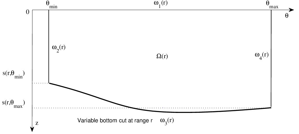
where obviously, ∂Ω(r)=∪i=14ωi(r)\partial\Omega(r)=\displaystyle{\cup_{i=1}^{4}}\omega_{i}(r) for ω1​(r):={(0,θ)∈ℝ2:θ∈[θmin,θmax]}\omega_{1}(r):=\{(0,\theta)\in\mathbb{R}^{2}:\;\theta\in[\theta_{\rm min},\theta_{\rm max}]\}, ω2​(r):={(z,θmin)∈ℝ2:z∈[0,s⁡(r,θmin)]}\omega_{2}(r):=\{(z,\theta_{\rm min})\in\mathbb{R}^{2}:\;z\in[0,s(r,\theta_{\rm min})]\}, ω3​(r):={(s⁡(r,θ),θ)∈ℝ2:θ∈[θmin,θmax]}\omega_{3}(r):=\{(s(r,\theta),\theta)\in\mathbb{R}^{2}:\;\theta\in[\theta_{\rm min},\theta_{\rm max}]\}, and ω4​(r):={(z,θmax)∈ℝ2:z∈[0,s⁡(r,θmax)]}\omega_{4}(r):=\{(z,\theta_{\rm max})\in\mathbb{R}^{2}:\;z\in[0,s(r,\theta_{\rm max})]\} (cf. Figure 1).

Refer to caption
Figure 1. The range dependent domain Ω⁡(r)\Omega(r).

The horizontal sea surface of the naval environment is assumed to be perfectly absorbing, so a free–release condition ψ=0\psi=0 is imposed on ω1​(r)\omega_{1}(r). We also set ψ=0\psi=0 on the minimum and maximum azimuthal values i.e. at ω2​(r)∪ω4​(r)\omega_{2}(r)\cup\omega_{4}(r). We denote by ωD​(r):=ω1​(r)∪ω2​(r)∪ω4​(r)\omega_{D}(r):=\omega_{1}(r)\cup\omega_{2}(r)\cup\omega_{4}(r) the piecewise linear boundary segment where these homogeneous Dirichlet conditions are imposed. The acoustically rigid bottom is mathematically modeled by the Neumann boundary condition ∂ψ∂ηs=0\frac{\partial\psi}{\partial\eta_{s}}=0 along the bottom surface z=s⁡(r,⋅)z=s(r,\cdot), i.e., the variable boundary segment ω3​(r)\omega_{3}(r) of Ω⁡(r)\Omega(r). Even in one space dimension, the well-posedness of the standard narrow–angle Parabolic Equation (1.1) with Neumann condition was proved under the assumption that the bottom topography is strictly monotone, cf. [1]. Considering the same problem, in [2, 8] the authors verified numerically that significant instabilities develop even in strictly monotone downsloping bottom profiles.

Abrahamsson and Kreiss in [1, 2] proposed alternatively the use of a Robin-type condition as an approximation of the Neumann one that yields a well-posed initial and boundary value problem when the domain topography is variable. This approximate condition in two dimensions has the form (cf. [24]):

(1.2) ψz−sθr2​ψθ=i​k0​sr​ψatz=s⁡(r,θ).\psi_{z}-\frac{s_{\theta}}{r^{2}}\psi_{\theta}=\mathrm{i}k_{0}s_{r}\psi\quad\text{at}\quad z=s(r,\theta).

We impose (1.2) at z=sz=s, we set in (1.1) a:=12​k0a:=\frac{1}{2k_{0}}, βψ​(r,z,θ):=k02​(n2−1)\beta_{\psi}(r,z,\theta):=\frac{k_{0}}{2}(n^{2}-1) and arrive at the following initial and boundary value problem (ibvp) of Schrödinger type:

(1.3) ψr=idiv(Da∇ψ)+iβψψinS,ψ=0on​ωD​(r)​∀r∈[rmin,rmax],ηst(Da∇ψ)=i2sr1+sθ2ψonω3(r)∀r∈[rmin,rmax],ψ⁡(rmin,z,θ)=ψ0​(z,θ)on​Ω​(rmin),\begin{split}&\psi_{r}=\mathrm{i\;div}(D_{\rm a}\nabla\psi)+\mathrm{i}\beta_{\psi}\psi\;\;\;\;\;\;\;\;\mbox{in}\;\;\;S,\\ &\psi=0\;\;\;\;\;\;\;\;\;\;\;\;\;\;\;\;\;\;\;\;\;\;\;\;\;\;\;\;\;\;\;\;\;\;\;\;\;\;\;\,\mbox{on}\;\;\;\omega_{D}(r)\;\;\;\forall r\in[r_{\rm min},r_{\rm max}],\\ &\eta_{\rm s}^{t}(D_{\rm a}\nabla\psi)=\frac{\mathrm{i}}{2}\frac{s_{r}}{\sqrt{1+s_{\theta}^{2}}}\psi\;\;\;\;\;\;\;\;\,\mbox{on}\;\;\;\omega_{3}(r)\;\;\;\forall r\in[r_{\rm min},r_{\rm max}],\\ &\psi(r_{\rm min},z,\theta)=\psi_{0}(z,\theta)\;\;\;\;\;\;\;\;\;\;\;\;\;\,\mbox{on}\;\;\;\Omega(r_{\rm min}),\end{split}

posed on the non-cylindrical domain S:=∪r∈[rmin,rmax]Ω(r)S:=\cup_{r\in[r_{\rm min},r_{\rm max}]}\Omega(r). Here, the gradient is with respect to the z,θz,\theta variables, Da:=(a00a/r2)D_{\rm a}:=\begin{pmatrix}{}_{a}&{}_{0}\\ {}_{0}&{}_{a/r^{2}}\end{pmatrix}, ηs=−(−1,sθ)t1+sθ2\eta_{\rm s}=-\frac{(-1,s_{\theta})^{t}}{\sqrt{1+s_{\theta}^{2}}} is the vector normal to the surface z=sz=s and the initial condition ψ0\psi_{0} models the acoustic source.

Remark 1.1.

In view of the ibvp (1.3), we observe that the same term Da∇ψD_{\rm a}\nabla\psi appears at the equation as well as at the left-hand side of the Abrahamsson-Kreiss Robin condition.

1.2. Change of variables

The focus of our interest herein is to write the problem into an equivalent form posed on a cylindrical domain where simpler stable numerical schemes can be applied. This is achieved by a horizontal change of variables combined with an exponential transformation. Specifically, we let

(1.4) y=z/s(r,θ),v(r,y,θ)=e−q⁡(r,θ)ψ(r,z,θ),Ω⁡(r)↪𝔇:=(0,1)×(θmin,θmax),S↪[rmin,rmax]×𝔇,\begin{split}&y=z/s(r,\theta),\;\;\;\;v(r,y,\theta)=e^{-q(r,\theta)}\psi(r,z,\theta),\\ &\Omega(r)\hookrightarrow\mathfrak{D}:=(0,1)\times(\theta_{\rm min},\theta_{\rm max}),\\ &S\hookrightarrow[r_{\rm min},r_{\rm max}]\times\mathfrak{D},\end{split}

where q⁡(r,θ)=−12​ln⁡s⁡(r,θ)q(r,\theta)=-\frac{1}{2}\ln s(r,\theta) [24, 6]. With this choice of qq, the initial- and boundary-value problem (1.3) takes the following form (see [6] for the details):

(1.5) vr=idiv(D^a∇v)+ysrsvy+iβvvin[rmin,rmax]×𝔇,v=0at​y=0​∀(r,θ)∈[rmin,rmax]×[θmin,θmax],ηt(D^a∇v)=iγbcvaty=1∀(r,θ)∈[rmin,rmax]×[θmin,θmax],v⁡(rmin,y,θ)=v0​(y,θ)∀(y,θ)∈𝔇¯,\begin{split}&v_{r}=\mathrm{i\;div}(\widehat{D}_{\rm a}\nabla v)+y\frac{s_{r}}{s}v_{y}+\mathrm{i}\beta_{v}v\;\;\;\;\;\;\;\;\mbox{in}\;\;\;[r_{\rm min},r_{\rm max}]\times\mathfrak{D},\\ &v=0\;\;\;\;\;\;\;\;\;\;\;\;\;\;\;\;\;\;\;\;\;\;\;\;\;\;\;\;\;\;\;\;\;\;\;\;\;\;\;\,\;\;\mbox{at}\;\;\;y=0\;\;\;\forall(r,\theta)\in[r_{\rm min},r_{\rm max}]\times[\theta_{\rm min},\theta_{\rm max}],\\ &\eta^{t}(\widehat{D}_{\rm a}\nabla v)=\mathrm{i}\gamma_{\rm bc}v\;\;\;\;\;\;\;\;\;\;\;\;\;\;\;\;\;\;\;\;\;\;\mbox{at}\;\;\;y=1\;\;\;\forall(r,\theta)\in[r_{\rm min},r_{\rm max}]\times[\theta_{\rm min},\theta_{\rm max}],\\ &v(r_{\rm min},y,\theta)=v_{0}(y,\theta)\;\;\;\;\;\;\;\;\;\;\;\;\;\,\;\;\forall(y,\theta)\in\overline{\mathfrak{D}},\end{split}

where η:=(1,0)t\eta:=(1,0)^{t}, γbc​(r,θ):=12​[srs+i​ar2​(sθs)2]\gamma_{\rm bc}(r,\theta):=\frac{\mathrm{1}}{2}\Big[\frac{s_{r}}{s}+\mathrm{i}\frac{a}{r^{2}}\Big(\frac{s_{\theta}}{s}\Big)^{2}\Big], and D^a:=(a^β^β^γ^)\widehat{D}_{\rm a}:=\begin{pmatrix}{}_{\widehat{a}}&{}_{\widehat{\beta}}\\ {}_{\widehat{\beta}}&{}_{\widehat{\gamma}}\end{pmatrix} with

a^(r,y,θ)=as2+ar2y2(sθs)2,β^(r,y,θ)=−ar2y(sθs),γ^(r)=ar2,\begin{split}\widehat{a}(r,y,\theta)=\frac{a}{s^{2}}+\frac{a}{r^{2}}y^{2}\Big(\frac{s_{\theta}}{s}\Big)^{2},\;\;\widehat{\beta}(r,y,\theta)=-\frac{a}{r^{2}}y\Big(\frac{s_{\theta}}{s}\Big),\;\;\widehat{\gamma}(r)=\frac{a}{r^{2}},\end{split}

βv:=βψ+ar2​3​sθ2−2​s​sθ​θ4​s2−i​sr2​s\beta_{v}:=\beta_{\psi}+\frac{a}{r^{2}}\frac{3s_{\theta}^{2}-2ss_{\theta\theta}}{4s^{2}}-\mathrm{i}\frac{s_{r}}{2s}, and v0​(y,θ)=s⁡(rmin,θ)​u0​(y​s​(rmin,θ),θ)v_{0}(y,\theta)=\sqrt{s(r_{\rm min},\theta)}u_{0}(ys(r_{\rm min},\theta),\theta).

We note that D^a\widehat{D}_{\rm a} is a real, symmetric and positive definite matrix and therefore det⁡(D^a)>0{\rm det}(\widehat{D}_{\rm a})>0, [6]. Furthermore, due to the definition of qq the coefficient of vyv_{y} in the first equation is a real function, which at y=1y=1 equals to 2​Re​γbc2{\rm Re}\gamma_{\rm bc}.

Certain three-dimensional effects have been observed to influence the acoustic transmission in variable domains mainly because the refraction index depends on rr, zz, θ\theta and since significant reflections may occur between the bottom and the see surface (cf. [19, 14, 27, 12, 13]). In [24], F. Sturm considered the Narrow–angle parabolic equation with the Abrahamsson-Kreiss condition in three dimensions over a variable bottom in the case of a multilayered fluid medium.

The single layer case in the presence of azimuthal symmetry where the physical problem is posed on one-dimensional variable domains has been analyzed rigorously in [5, 8]. More specifically, in [5] the authors constructed finite difference schemes and proved optimal rate of convergence. In [8], error estimates of optimal order in the L2L^{2}- and H1H^{1}-norms have been proved for semidiscrete and fully discrete Crank-Nicolson-Galerkin finite element approximations. Discontinuous Galerkin methods for the linear Schrödinger equation Dirichlet problem in non-cylindrical domains of ℝm\mathbb{R}^{m}, m≥1m\geq 1, were analyzed in [9]. When m=1m=1 the resulting problem is the standard Narrow–angle parabolic approximation modeling an acoustically soft bottom; for this case the authors investigated theoretically and numerically the order of convergence using finite element spaces of piecewise polynomial functions. The Wide–angle parabolic equation consists an alternative approximation model of Helmholtz equation in underwater acoustics; for a rigorous numerical analysis and numerical experiments on this model cf. [3, 4, 7, 16].

1.3. Generalization: The mathematical problem

Motivated by the properties of the physical problem, for the sake of a more general mathematical setting, in our analysis we consider the following initial- and boundary-value problem of Schrödinger type with variable coefficients and mixed boundary conditions (Dirichlet-Robin)

(1.6) ur=idiv(D∇u)+b∇u+iβu+Fin[rmin,rmax]×𝔇,u=0at​y=0​∀(r,θ)∈[rmin,rmax]×[θmin,θmax],ηt(D∇u)=iλuaty=1∀(r,θ)∈[rmin,rmax]×[θmin,θmax],u⁡(rmin,y,θ)=u0​(y,θ)∀(y,θ)∈𝔇¯.\begin{split}&u_{r}=\mathrm{i\;div}(D\nabla u)+b\nabla u+\mathrm{i}\beta u+F\;\;\;\;\;\;\;\;\mbox{in}\;\;\;[r_{\rm min},r_{\rm max}]\times\mathfrak{D},\\ &u=0\;\;\;\;\;\;\;\;\;\;\;\;\;\;\;\;\;\;\;\;\;\;\;\;\;\;\;\;\;\;\;\;\,\;\;\mbox{at}\;\;\;y=0\;\;\;\forall(r,\theta)\in[r_{\rm min},r_{\rm max}]\times[\theta_{\rm min},\theta_{\rm max}],\\ &\eta^{t}(D\nabla u)=\mathrm{i}\lambda u\;\;\;\;\;\;\;\;\;\;\;\;\;\;\;\;\;\;\;\mbox{at}\;\;\;y=1\;\;\;\forall(r,\theta)\in[r_{\rm min},r_{\rm max}]\times[\theta_{\rm min},\theta_{\rm max}],\\ &u(r_{\rm min},y,\theta)=u_{0}(y,\theta)\;\;\;\;\;\;\,\;\;\forall(y,\theta)\in\overline{\mathfrak{D}}.\end{split}

Here, 𝔇=(0,1)×(θmin,θmax)\mathfrak{D}=(0,1)\times(\theta_{\rm min},\theta_{\rm max}), η:=(1,0)t\eta:=(1,0)^{t}, while β=β⁡(r,y,θ)\beta=\beta(r,y,\theta), F=F⁡(r,y,θ)F=F(r,y,\theta) and λ=λ⁡(r,θ)\lambda=\lambda(r,\theta) are complex-valued functions.

For the rest of this paper, we shall assume that the following conditions are satisfied:

(1.7) D=D⁡(r,y,θ)​is a 2×2 real, symmetric matrix with​det​(D)>0∀r,y,θ,D=D(r,y,\theta)\;\text{is a $2\times 2$ real, symmetric matrix with}\;{\rm det}(D)>0\quad\forall\,r,y,\theta,
(1.8) b=(b1(r,y,θ),b2(r,y,θ))is real,b=\Big(b_{1}(r,y,\theta),\;b_{2}(r,y,\theta)\Big)\;\;\mbox{is real},

and

(1.9) b1​(r,1,θ)−2​Re​λ​(r,θ)≤0​∀r,θ.b_{1}(r,1,\theta)-2{\rm Re}\lambda(r,\theta)\leq 0\;\;\forall\,r,\theta.
Remark 1.2.

Since D∈ℝ2×2D\in\mathbb{R}^{2\times 2}, the condition (1.7) gives equivalently that DD is either positive or negative definite for any r,y,θr,y,\theta, which in turn relates to the ellipticity of the operator div(D∇⋅){\rm div}(D\nabla\cdot).

Remark 1.3.

As we shall prove later, the conditions (1.8) and (1.9) are sufficient for L2L^{2}-stability, while when (1.9) holds as equality the problem is H1H^{1}-stable also, cf. Theorem 3.1 and Remark 3.2.

Remark 1.4.

The form of the Robin boundary condition, considering only the first order terms, is related to the elliptic regularity of elliptic problems with mixed Dirichlet-Robin conditions in two dimensions proved in Theorem 4.3. The autonomous Section 4 of this paper presents a detailed proof of this argument.

Remark 1.5.

The acoustic problem (1.5) is a specific case of the problem (1.6) for u:=vu:=v, u0:=v0u_{0}:=v_{0}, D:=D^aD:=\widehat{D}_{\rm a}, b:=(y​srs,0)b:=(y\frac{s_{r}}{s},0), β:=βv\beta:=\beta_{v}, F:=0F:=0 and λ:=γbc\lambda:=\gamma_{\rm bc}, satisfying (1.7), (1.8), and (1.9) as equality, [6].

1.4. Main results

The problem analyzed here is motivated by an important physical application. Nevertheless, the general mathematical setting encompasses the very interesting aspect of approximating numerically a multi-dimensional ibvp of Schrödinger-type with mixed conditions and coefficients depending on the evolutionary variable.

In this paper, we apply the Galerkin method on the general problem (1.6) using piecewise polynomial finite element spaces. We construct fully discrete Crank–Nicolson-type schemes in rr for which we prove stability and optimal rate of accuracy in the L2L^{2}-norm. Numerical verification of the optimal rate of convergence is also presented.

The weak formulation of the problem is presented in Section 2. We define an appropriate rr-dependent sesquilinear form which is, in general, non-Hermitian. As it is common, the rate of accuracy is investigated by using certain properties of the projection induced by this form. The projection being rr-dependent and the fact that a two-dimensional rr-dependent Robin boundary condition appears in (1.6) make the analysis difficult. We estimate the projection error and its rr-derivative in the H1H^{1}- and L2L^{2}-norms (cf. paragraph 2.3, Propositions 2.3-2.5). The later is accomplished by applying an Elliptic Regularity Theorem for two-dimensional complex boundary value problems with mixed Dirichlet and Robin conditions, proved in Section 5. In the proof of Proposition 2.5, where the rr-derivative of the projection error is estimated in the L2L^{2}-norm, we present a very refined argument when treating the boundary terms.

In Section 3, we write (1.6) in a weak form and prove L2L^{2}-stability, and H1H^{1}-stability in the case where (1.9) holds as equality, so that the sesquilinear form is Hermitian. We then construct a fully discrete Crank-Nicolson scheme in range rr that is shown to be L2L^{2}-stable. Even though the evolutionary variable is discretized by a standard Crank-Nicolson method, the error analysis presented in this section is non-standard. This is due mainly to the fact that the form and the projection used are rr-dependent and calculated at the mid-points of a uniform range partition. We define properly a test function split in two terms involving projections applied on second order derivatives (cf. Remark 3.6), use the projection estimates of Section 2, and derive an optimal error estimate in the L2L^{2}-norm.

A general complex elliptic boundary value problem posed on a two-dimensional rectangular domain with mixed boundary conditions is analyzed in Section 4. If Dirichlet or Neumann conditions hold along the boundary, then in the weak formulation of the boundary value problem the trace integral terms vanish. A general approach of proving global regularity, [18], is to prove this estimate for half-balls, and then by change of variables, stretch the compact boundary locally and cover it by a finite union of half-balls. In our case, we analyze a complex elliptic problem posed on a rectangular domain of ℝ2\mathbb{R}^{2}. The boundary is compact and consists of four linear segments along which Dirichlet and Robin conditions are imposed. We apply directly on this domain the half-balls technique without change of variables as the boundary is already stretched locally. Further, we define appropriate test functions, in order to eliminate the trace terms from the weak formulation of the problem and prove the regularity estimate in Theorem 4.1. The result is extended in Theorem 4.3. Our proof covers a class of Robin conditions related to the coefficients of the pde of the boundary value problem, a special case of which is the Abrahamsson-Kreiss condition of underwater acoustics.

Finally, in Section 5 we report on the results of some numerical experiments performed with our method, verifying experimentally the optimal order of convergence.

2. An elliptic projection

2.1. Preliminaries

Let 𝔇=(0,1)×(θ1,θ2)\mathfrak{D}=(0,1)\times(\theta_{1},\theta_{2}). For rr in [rmin,rmax][r_{\rm min},r_{\rm max}] fixed, we define

∂y=y0:={(r,y0,θ)∈ℝ3:θ∈[θ1,θ2]},∂θ=θ0:={(r,y,θ0)∈ℝ3:y∈[0,1]},\partial_{y=y_{0}}:=\{(r,y_{0},\theta)\in\mathbb{R}^{3}:\theta\in[\theta_{1},\theta_{2}]\},\quad\partial_{\theta=\theta_{0}}:=\{(r,y,\theta_{0})\in\mathbb{R}^{3}:y\in[0,1]\},

and denote by H1​(𝔇)H^{1}(\mathfrak{D}) the associated usual (complex) Sobolev space. In order to deal with the Dirichlet boundary condition we shall make use of the space

H~01​(𝔇)={u∈H1​(𝔇):u|∂𝔇D=0},\tilde{H}_{0}^{1}(\mathfrak{D})=\{u\in H^{1}(\mathfrak{D}):u|_{\partial\mathfrak{D}_{D}}=0\},

where ∂𝔇D:=(∂y=0)∪(∂θ=θ1)∪(∂θ=θ2)\partial\mathfrak{D}_{D}:=(\partial_{y=0})\cup(\partial_{\theta=\theta_{1}})\cup(\partial_{\theta=\theta_{2}}). H~01​(𝔇)\tilde{H}_{0}^{1}(\mathfrak{D}) is the space of functions in H1​(𝔇)H^{1}(\mathfrak{D}) which vanish on y=0,θ=θ1,θ=θ2y=0,\theta=\theta_{1},\theta=\theta_{2}. We denote the L2​(𝔇)L^{2}(\mathfrak{D}) inner product by (⋅,⋅):L2​(𝔇)×L2​(𝔇)→ℂ(\cdot,\cdot):L^{2}(\mathfrak{D})\times L^{2}(\mathfrak{D})\rightarrow\mathbb{C}. ‖u‖:=(∫𝔇|u|2)12\|u\|:=\Big(\int_{\mathfrak{D}}|u|^{2}\Big)^{\frac{1}{2}} denotes the induced L2L^{2}-norm, while ‖u‖1:=(‖u‖2+‖uy‖2+‖uθ‖2)12\|u\|_{1}:=\Big(\|u\|^{2}+\|u_{y}\|^{2}+\|u_{\theta}\|^{2}\Big)^{\frac{1}{2}} is the usual H1​(𝔇)H^{1}(\mathfrak{D}) norm.

Let ∂𝔇R:=∂y=1\partial\mathfrak{D}_{R}:=\partial_{y=1} be the part of ∂𝔇\partial\mathfrak{D} where the Robin boundary condition of problem (1.6) is posed, and let

<u,v>:=∫θmaxθminu⁡(1,θ)​v¯​(1,θ)​𝑑θ,<u,v>:=\int_{\theta_{\rm max}}^{\theta_{\rm min}}u(1,\theta)\overline{v}(1,\theta)d\theta,

denote the inner product on H12​(∂𝔇R)H^{\frac{1}{2}}(\partial\mathfrak{D}_{R}). In addition, we shall make use of the norms:

|g|12,∂𝔇R:=infv∈H~01​(𝔇):v|∂𝔇R=g∥v∥1,|u|−12,∂𝔇R:=supv~∈H1​(𝔇),v~≠0|<u,v~>|‖v~‖1.\begin{split}&|g|_{\frac{1}{2},\partial\mathfrak{D}_{R}}:=\displaystyle{\inf_{v\in\tilde{H}_{0}^{1}(\mathfrak{D}):v|_{\partial\mathfrak{D}_{R}}=g}}\|v\|_{1},\\ &|u|_{-\frac{1}{2},\partial\mathfrak{D}_{R}}:=\displaystyle{\sup_{\tilde{v}\in H^{1}(\mathfrak{D}),\tilde{v}\neq 0}}\frac{|<u,\tilde{v}>|}{\|\tilde{v}\|_{1}}.\end{split}

Let τ∈ℕ\tau\in{\mathbb{N}} and ShS_{h} be a finite dimensional subspace of H~01​(𝔇)\tilde{H}_{0}^{1}(\mathfrak{D}) consisting of complex-valued functions that are polynomials of degree less than or equal to τ\tau in each interval of a non-uniform partition of 𝔇\mathfrak{D} with maximum length h∈(0,h⋆]h\in(0,h_{\star}]. It is well-known, [11], that the following approximation property holds:

(2.1) infχ∈Sh{‖v−χ‖+h​‖v−χ‖1}≤C​hs+1​‖v‖s+1,∀v∈Hs+1​(𝔇),∀h∈(0,h⋆],s=0,…,τ.\begin{split}\displaystyle{\inf_{\chi\in S_{h}}}\big\{\|v-\chi\|+h\|v-\chi\|_{1}\big\}\leq C\,h^{s+1}\,\|v\|_{s+1},\quad&\forall\,v\in H^{s+1}(\mathfrak{D}),\\ &\forall\,h\in(0,h_{\star}],\quad s=0,\dots,\tau.\end{split}

Also, we assume that the following inverse inequality holds:

(2.2) ‖ϕ‖1≤C​h−1​‖ϕ‖∀ϕ∈Sh,∀h∈(0,h⋆],\|\phi\|_{1}\leq\,C\,h^{-1}\,\|\phi\|\quad\forall\,\phi\in S_{h},\quad\forall\,h\in(0,h_{\star}],

which is true when, for example, the partition of 𝔇\mathfrak{D} is quasi-uniform, [11].

2.2. Definition of a sesquilinear form

Without loss of generality we assume that DD is positive definite. For any rr in [rmin,rmax][r_{\rm min},r_{\rm max}] we define the sesquilinear form ℬ⁡(r,⋅,⋅):H~01​(𝔇)×H~01​(𝔇)→ℂ\mathcal{B}(r;\cdot,\cdot):\tilde{H}_{0}^{1}(\mathfrak{D})\times\tilde{H}_{0}^{1}(\mathfrak{D})\rightarrow\mathbb{C}

(2.3) ℬ⁡(r,v,w):=(D(r)∇v,∇w)−i(∫θminθmaxλ(r,θ)v(1,θ)w¯(1,θ)dθ−(b(r)∇v,w))+δ⁡(v,w),\begin{split}\mathcal{B}(r;v,w):=&(D(r)\nabla v,\nabla w)-\mathrm{i}\Big(\int_{\theta_{\rm min}}^{\theta_{\rm max}}\lambda(r,\theta)v(1,\theta)\overline{w}(1,\theta)d\theta-(b(r)\nabla v,w)\Big)\\ &+\delta(v,w),\end{split}

for δ\delta a sufficiently large positive constant. Obviously, it holds that

(2.4) |ℬ⁡(r,v,w)|≤c​‖v‖1​‖w‖1,|\mathcal{B}(r;v,w)|\leq c\|v\|_{1}\|w\|_{1},

for any v,w∈H~01​(𝔇)v,w\in\tilde{H}_{0}^{1}(\mathfrak{D}), uniformly in rr.

We observe that (D∇v,∇v)≥c0∥∇v∥2(D\nabla v,\nabla v)\geq c_{0}\|\nabla v\|^{2} for a constant c0>0c_{0}>0 uniformly in rr and vv, since DD is real symmetric and positive definite. Therefore, by the trace inequality we obtain for v∈H~01​(𝔇)v\in\tilde{H}_{0}^{1}(\mathfrak{D})

Re​ℬ​(r,v,v)=(D(r)∇v,∇v)+δ∥v∥2+Im(∫θminθmaxλ(r,θ)v(1,θ)v¯(1,θ)dθ−(b(r)∇v,v))≥c0​‖∇v‖2+δ​‖v‖2−c2​‖v‖​‖v‖1.\begin{split}{\rm Re}\mathcal{B}(r;v,v)=&(D(r)\nabla v,\nabla v)+\delta\|v\|^{2}\\ &+{\rm Im}\Big(\int_{\theta_{\rm min}}^{\theta_{\rm max}}\lambda(r,\theta)v(1,\theta)\overline{v}(1,\theta)d\theta-(b(r)\nabla v,v)\Big)\\ \geq&c_{0}\|\nabla v\|^{2}+\delta\|v\|^{2}-c^{2}\|v\|\|v\|_{1}.\end{split}

Thus, by choosing δ\delta sufficiently large, it follows that there exists positive constant CC such that

(2.5) Re​ℬ​(r,v,v)≥C​‖v‖12,\begin{split}{\rm Re}\mathcal{B}(r;v,v)\geq C\|v\|_{1}^{2},\end{split}

uniformly, for any rr and any v∈H~01​(𝔇)v\in\tilde{H}_{0}^{1}(\mathfrak{D}).

Remark 2.1.

If DD is negative definite we may use

ℬn​(r,v,w):=−[(D(r)∇v,∇w)−i(∫θminθmaxλ(r,θ)v(1,θ)w¯(1,θ)dθ−(b(r)∇v,w))]+δ⁡(v,w),\begin{split}\mathcal{B}_{n}(r;v,w):=&-\Big[(D(r)\nabla v,\nabla w)-\mathrm{i}\Big(\int_{\theta_{\rm min}}^{\theta_{\rm max}}\lambda(r,\theta)v(1,\theta)\overline{w}(1,\theta)d\theta-(b(r)\nabla v,w)\Big)\Big]\\ &+\delta(v,w),\end{split}

with δ\delta a sufficiently large positive constant. In this case (2.4) and (2.5) also hold since now −D-D is positive definite.

2.3. Projection estimates

Let Rh​(r):H~01​(𝔇)→ShR_{h}(r):\tilde{H}_{0}^{1}(\mathfrak{D})\rightarrow S_{h} be a projection operator defined by

(2.6) ℬ⁡(r,Rh​(r)​v,ϕ)=ℬ⁡(r,v,ϕ)​∀ϕ∈Sh.\mathcal{B}(r;R_{h}(r)v,\phi)=\mathcal{B}(r;v,\phi)\;\;\forall\phi\in S_{h}.

Obviously, since (2.4) and (2.5) hold true, then by Lax-Milgram Theorem the projection is well defined.

Let us now define the operator

(2.7) ℒ∗(r)w:=−div(D∇w)+ib∇w+i[b1​y+b2​θ]w+δwin𝔇,w=0​on​∂𝔇D,ηt(D∇w)=iλ∗won∂𝔇R,\begin{split}&\mathcal{L}^{*}(r)w:=-{\rm div}(D\nabla w)+\mathrm{i}b\nabla w+\mathrm{i}[b_{1y}+b_{2\theta}]w+\delta w\;\;\mbox{in}\;\;\mathfrak{D},\\ &w=0\;\;\mbox{on}\;\;\partial\mathfrak{D}_{D},\\ &\eta^{t}(D\nabla w)=\mathrm{i}\lambda^{*}w\;\;\mbox{on}\;\;\partial\mathfrak{D}_{R},\end{split}

with λ∗\lambda^{*} a complex-valued function to be chosen appropriately in the sequel. For ϕ∈H~01​(𝔇)\phi\in\tilde{H}_{0}^{1}(\mathfrak{D}) we get

(2.8) (ℒ∗​(r)​w,ϕ)=(D∇w,∇ϕ)−∫θminθmaxiλ∗w(1)ϕ¯(1)dθ+i(b∇w,ϕ)+i([b1​y+b2​θ]w,ϕ)+δ(w,ϕ)=(D∇w,∇ϕ)−∫θminθmaxiλ∗w(1)ϕ¯(1)dθ−i⁡([b1​y+b2​θ]​w,ϕ)−i⁡(b​w,∇ϕ)+i​∫θminθmaxb1​(1)​w​(1)​ϕ¯​(1)​𝑑θ+i⁡([b1​y+b2​θ]​w,ϕ)+δ⁡(w,ϕ)=(D∇w,∇ϕ)+i∫θminθmax[b1(1)−λ∗]w(1)ϕ¯(1)dθ−i(bw,∇ϕ)+δ(w,ϕ).\begin{split}(\mathcal{L}^{*}(r)w,\phi)&=(D\nabla w,\nabla\phi)-\int_{\theta_{\rm min}}^{\theta_{\rm max}}\mathrm{i}\lambda^{*}w(1)\overline{\phi}(1)d\theta\\ &\quad+\mathrm{i}(b\nabla w,\phi)+\mathrm{i}([b_{1y}+b_{2\theta}]w,\phi)+\delta(w,\phi)\\ &=(D\nabla w,\nabla\phi)-\int_{\theta_{\rm min}}^{\theta_{\rm max}}\mathrm{i}\lambda^{*}w(1)\overline{\phi}(1)d\theta\\ &\quad-\mathrm{i}([b_{1y}+b_{2\theta}]w,\phi)-\mathrm{i}(bw,\nabla\phi)+\mathrm{i}\int_{\theta_{\rm min}}^{\theta_{\rm max}}b_{1}(1)w(1)\overline{\phi}(1)d\theta\\ &\quad+\mathrm{i}([b_{1y}+b_{2\theta}]w,\phi)+\delta(w,\phi)\\ &=(D\nabla w,\nabla\phi)+\mathrm{i}\int_{\theta_{\rm min}}^{\theta_{\rm max}}[b_{1}(1)-\lambda^{*}]w(1)\overline{\phi}(1)d\theta-\mathrm{i}(bw,\nabla\phi)+\delta(w,\phi).\end{split}

Since DD, bb and δ\delta are real, then for any ϕ\phi in H~01​(𝔇)\tilde{H}_{0}^{1}(\mathfrak{D}) it follows that

(2.9) (ℒ∗​(r)​w,ϕ)¯=(D∇ϕ,∇w)−i∫θminθmax[b1(1)−λ∗¯]ϕ(1)w¯(1)dθ+i(b∇ϕ,w)+δ(ϕ,w).\begin{split}\overline{(\mathcal{L}^{*}(r)w,\phi)}&=(D\nabla\phi,\nabla w)-\mathrm{i}\int_{\theta_{\rm min}}^{\theta_{\rm max}}[b_{1}(1)-\overline{\lambda^{*}}]\phi(1)\overline{w}(1)d\theta\\ &\quad+\mathrm{i}(b\nabla\phi,w)+\delta(\phi,w).\end{split}

Setting

(2.10) λ∗:=b1​(1)−λ¯,\lambda^{*}:=b_{1}(1)-\overline{\lambda},

we obtain

(2.11) (ℒ∗​(r)​w,ϕ)¯=ℬ⁡(r,ϕ,w),\begin{split}\overline{(\mathcal{L}^{*}(r)w,\phi)}=\mathcal{B}(r;\phi,w),\end{split}

and thus

(2.12) (ℒ∗​(r)​w,ϕ)=ℬ⁡(r,ϕ,w)¯,\begin{split}(\mathcal{L}^{*}(r)w,\phi)=\overline{\mathcal{B}(r;\phi,w)},\end{split}

for any ϕ∈H~01​(𝔇)\phi\in\tilde{H}_{0}^{1}(\mathfrak{D}). Throughout the rest of this paper, we consider λ∗\lambda^{*} given by (2.10).

Remark 2.2.

We observe that in the case of the specific problem (1.5), b1=y​srsb_{1}=y\frac{s_{r}}{s}, b2=0b_{2}=0, λ=12​[srs+i​ar2​(sθs)2]\lambda=\frac{\mathrm{1}}{2}\Big[\frac{s_{r}}{s}+\mathrm{i}\frac{a}{r^{2}}\Big(\frac{s_{\theta}}{s}\Big)^{2}\Big] and thus

λ∗=b1​(1)−λ¯=srs−12​[srs−i​ar2​(sθs)2]=λ.\lambda^{*}=b_{1}(1)-\overline{\lambda}=\frac{s_{r}}{s}-\frac{\mathrm{1}}{2}\Big[\frac{s_{r}}{s}-\mathrm{i}\frac{a}{r^{2}}\Big(\frac{s_{\theta}}{s}\Big)^{2}\Big]=\lambda.
Proposition 2.3.

There exists a positive constant cc such that if v∈H~01​(𝔇)∩Hs​(𝔇)v\in\tilde{H}_{0}^{1}(\mathfrak{D})\cap H^{s}(\mathfrak{D}) then

(2.13) ‖Rh​(r)​v−v‖1≤c​hτ​‖v‖τ+1,\begin{split}\|R_{h}(r)v-v\|_{1}\leq ch^{\tau}\|v\|_{\tau+1},\end{split}

and

(2.14) ‖Rh​(r)​v−v‖≤c​hτ+1​‖v‖τ+1.\begin{split}\|R_{h}(r)v-v\|\leq ch^{\tau+1}\|v\|_{\tau+1}.\end{split}
Proof.

We set e:=Rh​(r)​v−ve:=R_{h}(r)v-v, use (2.5), (2.4) and (2.1) to obtain for ϕ∈Sh\phi\in S_{h}

c​‖e‖12≤Re​ℬ​(r,e,e)=Re​ℬ​(r,e,Rh​(r)​v−v)=Re​ℬ​(r,e,ϕ−v)≤c​‖e‖1​infϕ∈Sh‖ϕ−v‖1≤c​‖e‖1​hτ​‖v‖τ+1,\begin{split}c\|e\|_{1}^{2}\leq{\rm Re}\mathcal{B}(r;e,e)&={\rm Re}\mathcal{B}(r;e,R_{h}(r)v-v)={\rm Re}\mathcal{B}(r;e,\phi-v)\\ &\leq c\|e\|_{1}\displaystyle{\inf_{\phi\in S_{h}}}\|\phi-v\|_{1}\leq c\|e\|_{1}h^{\tau}\|v\|_{\tau+1},\end{split}

which establishes (2.13).

Let now ww be the solution of the problem: ℒ∗​(r)​w=e\mathcal{L}^{*}(r)w=e. Then by using (2.12), the approximation property and elliptic regularity, proved in Theorem 4.3, we get for ϕ∈Sh\phi\in S_{h}:

‖e‖2=(ℒ∗​(r)​w,e)=ℬ⁡(r,e,w)¯=ℬ⁡(r,e,w−ϕ)¯≤c​‖e‖1​infϕ∈Sh‖w−ϕ‖1≤c​hτ​‖v‖τ+1​h​‖w‖2≤c​hτ+1​‖v‖τ+1​‖e‖,\begin{split}\|e\|^{2}=(\mathcal{L}^{*}(r)w,e)&=\overline{\mathcal{B}(r;e,w)}=\overline{\mathcal{B}(r;e,w-\phi)}\\ &\leq c\|e\|_{1}\displaystyle{\inf_{\phi\in S_{h}}}\|w-\phi\|_{1}\leq ch^{\tau}\|v\|_{\tau+1}h\|w\|_{2}\leq ch^{\tau+1}\|v\|_{\tau+1}\|e\|,\end{split}

which yields (2.14). ∎

Proposition 2.4.

Let r∈C1​([rmin,rmax],Hr​(𝔇))r\in C^{1}([r_{\rm min},r_{\rm max}],H^{{\rm r}}(\mathfrak{D})). Then it holds that

(2.15) ‖∂r(Rh​(r)​v​(r)−v⁡(r))‖1≤C​hτ​(‖v‖τ+1+‖∂rv‖τ+1).\left\|\partial_{r}\left(R_{h}(r)v(r)-v(r)\right)\right\|_{1}\leq\,C\,h^{\tau}\,\left(\,\|v\|_{\tau+1}+\|\partial_{r}v\|_{\tau+1}\,\right).
Proof.

We set e:=Rh​(r)​v​(r)−v⁡(r)e:=R_{h}(r)v(r)-v(r). Let v:[rmin,rmax]→Hr​(𝔇)v:[r_{\rm min},r_{\rm max}]\rightarrow H^{{\rm r}}(\mathfrak{D}) and e⁡(r)=Rh​(r)​v​(r)−v⁡(r)e(r)=R_{h}(r)v(r)-v(r) for r∈[rmin,rmax]r\in[r_{\rm min},r_{\rm max}]. Then, we have

ℬ⁡(r,e⁡(r),ϕ)=0​∀ϕ∈Sh.\mathcal{B}(r;e(r),\phi)=0\;\;\forall\phi\in S_{h}.

Differentiating the above relation with respect to rr we obtain

ℬ⁡(r,e˙​(r),ϕ)+ℬ˙​(r,e⁡(r),ϕ)=0​∀ϕ∈Sh.\mathcal{B}(r;\dot{e}(r),\phi)+\dot{\mathcal{B}}(r;e(r),\phi)=0\;\;\forall\phi\in S_{h}.

Now, for ϕ∈Sh\phi\in S_{h} we have

c​‖e˙​(r)‖12≤ℬ⁡(r,e˙​(r),e˙​(r))=ℬ⁡(r,e˙​(r),e˙​(r)+ϕ)−ℬ⁡(r,e˙​(r),ϕ)=ℬ⁡(r,e˙​(r),e˙​(r)+ϕ)+ℬ⁡(r,e⁡(r),ϕ)≤c⁡[‖e˙​(r)‖1​‖e˙​(r)+ϕ‖1+‖e⁡(r)‖1​‖ϕ‖1]≤c⁡[‖e˙​(r)‖1​‖e˙​(r)+ϕ‖1+‖e⁡(r)‖1​(‖e˙​(r)+ϕ‖1+‖e˙​(r)‖1)]=c⁡[(‖e˙​(r)‖1+‖e⁡(r)‖1)​‖e˙​(r)+ϕ‖1+‖e⁡(r)‖1​‖e˙​(r)‖1]≤c⁡[(‖e˙​(r)‖1+‖e⁡(r)‖1)​infϕ∈Sh‖∂r(Rh​v)​(r)−∂rv+ϕ‖1+‖e⁡(r)‖1​‖e˙​(r)‖1]≤c⁡[(‖e˙​(r)‖1+‖e⁡(r)‖1)​infϕ∈Sh‖∂rv−ϕ‖1+‖e⁡(r)‖1​‖e˙​(r)‖1]=c​‖e˙​(r)‖1​[‖e⁡(r)‖1+infϕ∈Sh‖∂rv−ϕ‖1]+c|e⁡(r)|infϕ∈Sh1⁡‖∂rv−ϕ‖1.\begin{split}c\|\dot{e}(r)\|_{1}^{2}&\leq\mathcal{B}(r;\dot{e}(r),\dot{e}(r))=\mathcal{B}(r;\dot{e}(r),\dot{e}(r)+\phi)-\mathcal{B}(r;\dot{e}(r),\phi)\\ &=\mathcal{B}(r;\dot{e}(r),\dot{e}(r)+\phi)+\mathcal{B}(r;e(r),\phi)\\ &\leq c\Big[\|\dot{e}(r)\|_{1}\|\dot{e}(r)+\phi\|_{1}+\|e(r)\|_{1}\|\phi\|_{1}\Big]\\ &\leq c\Big[\|\dot{e}(r)\|_{1}\|\dot{e}(r)+\phi\|_{1}+\|e(r)\|_{1}(\|\dot{e}(r)+\phi\|_{1}+\|\dot{e}(r)\|_{1})\Big]\\ &=c\Big[(\|\dot{e}(r)\|_{1}+\|e(r)\|_{1})\|\dot{e}(r)+\phi\|_{1}+\|e(r)\|_{1}\|\dot{e}(r)\|_{1}\Big]\\ &\leq c\Big[(\|\dot{e}(r)\|_{1}+\|e(r)\|_{1})\displaystyle{\inf_{\phi\in S_{h}}}\|\partial_{r}(R_{h}v)(r)-\partial_{r}v+\phi\|_{1}+\|e(r)\|_{1}\|\dot{e}(r)\|_{1}\Big]\\ &\leq c\Big[(\|\dot{e}(r)\|_{1}+\|e(r)\|_{1})\displaystyle{\inf_{\phi\in S_{h}}}\|\partial_{r}v-\phi\|_{1}+\|e(r)\|_{1}\|\dot{e}(r)\|_{1}\Big]\\ &=c\|\dot{e}(r)\|_{1}\Big[\|e(r)\|_{1}+\displaystyle{\inf_{\phi\in S_{h}}}\|\partial_{r}v-\phi\|_{1}\Big]+c\|e(r)\|_{1}\displaystyle{\inf_{\phi\in S_{h}}}\|\partial_{r}v-\phi\|_{1}.\end{split}

The claim of the proposition follows by using the approximation property 2.1 with s=τ+1s=\tau+1. ∎

Using a technique introduced in [17], we are able to show the following optimal order approximation result for the time-derivative of the elliptic projection.

Proposition 2.5.

There exists a positive constant cc such that

(2.16) ‖∂r(Rh​(r)​v​(r)−v⁡(r))‖≤C​hτ+1​(‖v‖τ+1+‖∂rv‖τ+1).\left\|\partial_{r}\left(R_{h}(r)v(r)-v(r)\right)\right\|\leq C\,h^{\tau+1}\,\left(\,\|v\|_{\tau+1}+\|\partial_{r}v\|_{\tau+1}\,\right).
Proof.

We set e:=Rh​(r)​v​(r)−v⁡(r)e:=R_{h}(r)v(r)-v(r). Let ww be the solution of the problem: ℒ∗​w=e˙\mathcal{L}^{*}w=\dot{e}. For χ∈Sh\chi\in S_{h} we have

‖e˙​(r)‖2=(ℒ∗​w,e˙​(r))=ℬ​(r,e˙​(r),w)¯=Re⁡[ℬ​(r,e˙​(r),w−χ)¯−ℬ˙​(r,e,χ)¯]≤c⁡[‖e˙​(r)‖1​‖w−χ‖1+‖e⁡(r)‖1​‖w−χ‖1]−Re⁡[ℬ˙​(r,e,w)]≤c⁡(‖e˙​(r)‖1+‖e⁡(r)‖)​infχ∈Sh‖w−χ‖1−Re⁡[ℬ˙​(r,e,w)]≤c​hr​(‖v‖r+1+‖∂rv‖r+1)​h​‖w‖2−Re⁡[ℬ˙​(r,e,w)].\begin{split}\|\dot{e}(r)\|^{2}&=(\mathcal{L}^{*}w,\dot{e}(r))=\overline{\mathcal{B}(r;\dot{e}(r),w)}\\ &={\rm Re}\Big[\overline{\mathcal{B}(r;\dot{e}(r),w-\chi)}-\overline{\dot{\mathcal{B}}(r;e,\chi)}\Big]\\ &\leq c\Big[\|\dot{e}(r)\|_{1}\|w-\chi\|_{1}+\|e(r)\|_{1}\|w-\chi\|_{1}\Big]-{\rm Re}\Big[\dot{\mathcal{B}}(r;e,w)\Big]\\ &\leq c\Big(\|\dot{e}(r)\|_{1}+\|e(r)\|\Big)\displaystyle{\inf_{\chi\in S_{h}}}\|w-\chi\|_{1}-{\rm Re}\Big[\dot{\mathcal{B}}(r;e,w)\Big]\\ &\leq ch^{\rm r}\Big(\|v\|_{\rm r+1}+\|\partial_{r}v\|_{\rm r+1}\Big)h\|w\|_{2}-{\rm Re}\Big[\dot{\mathcal{B}}(r;e,w)\Big].\end{split}

For convenience we set I:=Re​[ℬ˙​(r,e,w)]I:={\rm Re}\Big[\dot{\mathcal{B}}(r;e,w)\Big]. First, observe that

ℬ˙(r;e,w)=(∂rD∇e,∇w)−i(∫θminθmax∂rλ(r,θ)e(r,1,θ)w¯(r,1,θ)dθ−(∂rb∇e,w)),\dot{\mathcal{B}}(r;e,w)=(\partial_{r}D\nabla e,\nabla w)-\mathrm{i}\Big(\int_{\theta_{\rm min}}^{\theta_{\rm max}}\partial_{r}\lambda(r,\theta)e(r,1,\theta)\overline{w}(r,1,\theta)d\theta-(\partial_{r}b\nabla e,w)\Big),

so that

I=Re[(∂rD∇e,∇w)−i(∫θminθmax∂rλ(r,θ)e(r,1,θ)w¯(r,1,θ)dθ−(∂rb∇e,w))].I={\rm Re}\Big[(\partial_{r}D\nabla e,\nabla w)-\mathrm{i}\Big(\int_{\theta_{\rm min}}^{\theta_{\rm max}}\partial_{r}\lambda(r,\theta)e(r,1,\theta)\overline{w}(r,1,\theta)d\theta-(\partial_{r}b\nabla e,w)\Big)\Big].

By the definition of the inner product <u,v><u,v> we have

I1:=Re[i(∂rb∇e,w)]=Re[−i⁡(∂r[b1​y+b2​θ]​e,w)−i⁡(∂rb​e,∇w)+i∫θminθmax(∂rb1)(1)e(1)w¯(1)dθ]≤c|e|‖w‖1+Re⁡[i⁡<∂rb1​e,w>].\begin{split}I_{1}:={\rm Re}\Big[\mathrm{i}(\partial_{r}b\nabla e,w)\Big]={\rm Re}\Big[&-\mathrm{i}(\partial_{r}[b_{1y}+b_{2\theta}]e,w)-\mathrm{i}(\partial_{r}be,\nabla w)\\ &+\mathrm{i}\int_{\theta_{\rm min}}^{\theta_{\rm max}}(\partial_{r}b_{1})(1)e(1)\overline{w}(1)d\theta\Big]\\ &\leq c\|e\|\|w\|_{1}+{\rm Re}\Big[\mathrm{i}<\partial_{r}b_{1}e,w>\Big].\end{split}

We set I2:=Re[−i∫θminθmax∂rλew¯dθ]I_{2}:={\rm Re}\Big[-\mathrm{i}\int_{\theta_{\rm min}}^{\theta_{\rm max}}\partial_{r}\lambda e\overline{w}d\theta\Big]. Using the estimates above we obtain

I1+I2≤Re⁡[−i⁡<[∂rλ−∂rb1]​e,w>]+c​‖e‖​‖w‖1≤c​|e|−12,∂𝔇R​‖w‖1+c|e|‖w‖1≤c⁡[‖e‖+|e|−12,∂𝔇R]​‖w‖1.\begin{split}I_{1}+I_{2}&\leq{\rm Re}\Big[-\mathrm{i}<[\partial_{r}\lambda-\partial_{r}b_{1}]e,w>\Big]+c\|e\|\|w\|_{1}\\ &\leq c|e|_{-\frac{1}{2},\partial\mathfrak{D}_{R}}\|w\|_{1}+c\|e\|\|w\|_{1}\leq c\Big[\|e\|+|e|_{-\frac{1}{2},\partial\mathfrak{D}_{R}}\Big]\|w\|_{1}.\end{split}

In addition,

I3:=Re[(∂rD∇e,∇w)]=Re[∫θminθmaxη(∂rD∇we¯)dθ−(div(∂rD∇w),e)]≤c∥w∥2∥e∥+Re[<η(∂rD∇w),e>]≤c​‖w‖2|e|+|e|−12,∂𝔇R​‖w‖2≤c⁡[‖e‖+|e|−12,∂𝔇R]​‖w‖2,\begin{split}I_{3}&:={\rm Re}\Big[(\partial_{r}D\nabla e,\nabla w)\Big]={\rm Re}\Big[\int_{\theta_{\rm min}}^{\theta_{\rm max}}\eta(\partial_{r}D\nabla w\overline{e})d\theta-({\rm div}(\partial_{r}D\nabla w),e)\Big]\\ &\leq c\|w\|_{2}\|e\|+{\rm Re}\Big[<\eta(\partial_{r}D\nabla w),e>\Big]\\ &\leq c\|w\|_{2}\|e\|+|e|_{-\frac{1}{2},\partial\mathfrak{D}_{R}}\|w\|_{2}\leq c\Big[\|e\|+|e|_{-\frac{1}{2},\partial\mathfrak{D}_{R}}\Big]\|w\|_{2},\end{split}

so that

(2.17) I≤c⁡[‖e‖+|e|−12,∂𝔇R]​‖w‖2.I\leq c\Big[\|e\|+|e|_{-\frac{1}{2},\partial\mathfrak{D}_{R}}\Big]\|w\|_{2}.

Now, for g∈H12​(∂𝔇R)g\in H^{\frac{1}{2}}(\partial\mathfrak{D}_{R}) we consider the elliptic problem

−div(D∇z)+ib∇z+i[b1​y+b2​θ]z+δz=0in𝔇,z=0​on​∂𝔇D,ηt(D∇z)=iλ∗z+gon∂𝔇R.\begin{split}&-{\rm div}(D\nabla z)+\mathrm{i}b\nabla z+\mathrm{i}[b_{1y}+b_{2\theta}]z+\delta z=0\;\;\mbox{in}\;\;\mathfrak{D},\\ &z=0\;\;\mbox{on}\;\;\partial\mathfrak{D}_{D},\\ &\eta^{t}(D\nabla z)=\mathrm{i}\lambda^{*}z+g\;\;\mbox{on}\;\;\partial\mathfrak{D}_{R}.\end{split}

Then we have 0=ℬ⁡(r,e⁡(r),z)¯−<g,e>0=\overline{\mathcal{B}(r;e(r),z)}-<g,e> and thus,

<g,e>=ℬ⁡(r,e⁡(r),z)¯=ℬ⁡(r,e⁡(r),z−ϕ)¯​∀ϕ∈Sh.\begin{split}<g,e>=\overline{\mathcal{B}(r;e(r),z)}=\overline{\mathcal{B}(r;e(r),z-\phi)}\;\;\forall\phi\in S_{h}.\end{split}

It follows then that

|<e,g>|≤c​‖e‖1​infϕ∈Sh‖z−ϕ‖1,\begin{split}|<e,g>|\leq c\|e\|_{1}\displaystyle{\inf_{\phi\in S_{h}}}\|z-\phi\|_{1},\end{split}

and therefore,

|<e,g>|≤c​hτ​‖v‖τ+1​h​‖z‖2.|<e,g>|\leq ch^{\tau}\|v\|_{\tau+1}h\|z\|_{2}.

The elliptic regularity result (cf. Theorem 4.3 and Remark 4.4) for the solution zz of the elliptic problem above, reads

‖z‖2≤c​|g|12,∂𝔇R.\|z\|_{2}\leq c|g|_{\frac{1}{2},\partial\mathfrak{D}_{R}}.

Thus we have

|e|−12,∂𝔇R:=supv~∈H1​(𝔇),v~≠0|<e,v~>|‖v~‖1≤c​hτ+1​‖v‖τ+1,|e|_{-\frac{1}{2},\partial\mathfrak{D}_{R}}:=\displaystyle{\sup_{\tilde{v}\in H^{1}(\mathfrak{D}),\tilde{v}\neq 0}}\frac{|<e,\tilde{v}>|}{\|\tilde{v}\|_{1}}\leq ch^{\tau+1}\|v\|_{\tau+1},

and subsequently, using the elliptic regularity of ww, cf. again Theorem 4.3, we arrive at

‖e˙​(r)‖2≤chτ+1(∥v∥τ+1+∥∂rv∥τ+1)∥w∥2+c[∥e∥+|e|−1/2,∂𝔇R]∥w∥2≤c​‖w‖2​hτ+1​(‖v‖τ+1+‖∂rv‖τ+1)≤c​‖e˙​(r)‖​hτ+1​(‖v‖τ+1+‖∂rv‖τ+1),\begin{split}\|\dot{e}(r)\|^{2}&\leq ch^{\tau+1}\Big(\|v\|_{\tau+1}+\|\partial_{r}v\|_{\tau+1}\Big)\|w\|_{2}+c\Big[\|e\|+|e|_{-1/2,\partial\mathfrak{D}_{R}}\Big]\|w\|_{2}\\ &\leq c\|w\|_{2}h^{\tau+1}\Big(\|v\|_{\tau+1}+\|\partial_{r}v\|_{\tau+1}\Big)\leq c\|\dot{e}(r)\|h^{\tau+1}\Big(\|v\|_{\tau+1}+\|\partial_{r}v\|_{\tau+1}\Big),\end{split}

which completes the proof of the proposition. ∎

3. A Crank–Nikolson-type fully discrete scheme

3.1. Weak Formulation

Let ϕ∈H~01​(𝔇)\phi\in\tilde{H}_{0}^{1}(\mathfrak{D}). Multiplying the partial differential equation of (1.6) by ϕ¯\bar{\phi} and integrating by parts we have

(3.1) (ur(r),ϕ)=i[−(D(r)∇u(r),∇ϕ)+∫∂𝔇ηtD(r)∇u(r)ϕ¯ds]+(b(r)∇u(r),ϕ)+i⁡(β⁡(r)​u​(r),ϕ)+(F⁡(r),ϕ)=−i[(D(r)∇u(r),∇ϕ)−i{∫θminθmaxλ(r,θ)u(r,1,θ)ϕ¯(1,θ)dθ−(b(r)∇u(r),ϕ)}]+i⁡(β⁡(r)​u​(r),ϕ)+(F⁡(r),ϕ)=−i​ℬ​(r,u⁡(r),ϕ)+i⁡((β⁡(r)+δ)​u​(r),ϕ)+(F⁡(r),ϕ),\begin{split}&\Big(u_{r}(r),\phi\Big)=\mathrm{i}\Big[-\Big(D(r)\nabla u(r),\nabla\phi\Big)+\int_{\partial\mathfrak{D}}\eta^{t}D(r)\nabla u(r)\overline{\phi}ds\Big]+\Big(b(r)\nabla u(r),\phi\Big)\\ &+\mathrm{i}\Big(\beta(r)u(r),\phi\Big)+(F(r),\phi)\\ &=-\mathrm{i}\Big[\Big(D(r)\nabla u(r),\nabla\phi\Big)-\mathrm{i}\Big\{\int_{\theta_{\rm min}}^{\theta_{\rm max}}\lambda(r,\theta)u(r,1,\theta)\overline{\phi}(1,\theta)d\theta-\Big(b(r)\nabla u(r),\phi\Big)\Big\}\Big]\\ &+\mathrm{i}\Big(\beta(r)u(r),\phi\Big)+(F(r),\phi)\\ &=-\mathrm{i}\mathcal{B}\Big(r;u(r),\phi\Big)+\mathrm{i}\Big((\beta(r)+\delta)u(r),\phi\Big)+(F(r),\phi),\end{split}

for any ϕ∈H~01​(𝔇)\phi\in\tilde{H}_{0}^{1}(\mathfrak{D}). In the following theorem we prove that (3.1) defines uu in H~01​(𝔇)\tilde{H}_{0}^{1}(\mathfrak{D}) uniquely.

Theorem 3.1.

The weak problem (3.1) has at most one solution in H~01​(𝔇)\tilde{H}_{0}^{1}(\mathfrak{D}).

Proof.

Let u∈H~01​(𝔇)u\in\tilde{H}_{0}^{1}(\mathfrak{D}) be a solution of (3.1). We set ϕ=u\phi=u in (3.1), integrate by parts, use the facts that DD is a real, symmetric matrix, that bb is real, and take real parts. More specifically, we obtain first

(3.2) (ur,u)=−i[(D∇u,∇u)−i(∫θminθmaxλ(r,θ)u(r,1,θ)u¯(1,θ)dθ−(b∇u,u))]+i⁡(β​u,u)+(F,u).\begin{split}(u_{r},u)=&-\mathrm{i}\Big[(D\nabla u,\nabla u)-\mathrm{i}\Big(\int_{\theta_{\rm min}}^{\theta_{\rm max}}\lambda(r,\theta)u(r,1,\theta)\overline{u}(1,\theta)d\theta-(b\nabla u,u)\Big)\Big]\\ &+\mathrm{i}(\beta u,u)+(F,u).\end{split}

Observe that

Re(b∇u,u)=−12(b1​yu,u)−12(b2​θu,u)+12∫θminθmaxb1(r,1,θ)|u(r,1,θ)|2dθ,{\rm Re}(b\nabla u,u)=-\frac{1}{2}(b_{1y}u,u)-\frac{1}{2}(b_{2\theta}u,u)+\frac{1}{2}\int_{\theta_{\rm min}}^{\theta_{\rm max}}b_{1}(r,1,\theta)|u(r,1,\theta)|^{2}d\theta,

since bb is real and u=0u=0 at y=0y=0, θ=θmin,θmax\theta=\theta_{\rm min},\theta_{\rm max}. Since DD is real, then using this observation in (3.2) we arrive at

12​dd​r​‖u‖2=∫θminθmax[−Re​λ​(r,θ)+12​b1​(r,1,θ)]​|u⁡(r,1,θ)|2​𝑑θ−12​([b1​y+b2​θ]​u,u)−(Im⁡(β)​u,u)+Re⁡(F,u).\begin{split}\frac{1}{2}\frac{d}{dr}\|u\|^{2}=&\int_{\theta_{\rm min}}^{\theta_{\rm max}}[-{\rm Re}\lambda(r,\theta)+\frac{1}{2}b_{1}(r,1,\theta)]|u(r,1,\theta)|^{2}d\theta\\ &-\frac{1}{2}([b_{1y}+b_{2\theta}]u,u)-({\rm Im}(\beta)u,u)+{\rm Re}(F,u).\end{split}

Using the condition (1.9) and Grönwall’s inequality we obtain the stability estimate

(3.3) ‖u‖≤c​‖u0‖+c​∫rminrmax‖F‖​dr.\left.\begin{array}[]{l}\|u\|\leq c\|u_{0}\|+c\int_{r_{\rm min}}^{r_{\rm max}}\|F\|\,dr.\end{array}\right.

Uniqueness of the solution uu follows readily from the estimate above. ∎

Remark 3.2.

If (1.9) holds as equality then the sesquilinear form is Hermitian. Therefore, if F=0F=0, using (3.1), setting ϕ=ur−i⁡(β+δ)​u\phi=u_{r}-{\rm i}(\beta+\delta)u and taking imaginary parts we obtain

12​dd​t​Re​ℬ​(r,u⁡(r),u⁡(r))≤c1​‖u‖12≤c​Re​ℬ​(r,u⁡(r),u⁡(r)),\begin{split}\frac{1}{2}\frac{d}{dt}{\rm Re}\mathcal{B}(r;u(r),u(r))\leq c_{1}\|u\|_{1}^{2}\leq c{\rm Re}\mathcal{B}(r;u(r),u(r)),\end{split}

so that c​‖u‖12≤Re​ℬ​(r,u⁡(r),u⁡(r))≤c​‖u0‖12c\|u\|_{1}^{2}\leq{\rm Re}\mathcal{B}(r;u(r),u(r))\leq c\|u_{0}\|_{1}^{2}, i.e. we also obtain an H1H^{1} stability estimate.

Remark 3.3.

Note that for the specific case of problem (1.5), if βψ\beta_{\psi} is real, we have F=0F=0, Im⁡(β):=Im⁡(βv)=−sr2​s{\rm Im}(\beta):={\rm Im}(\beta_{v})=-\frac{s_{r}}{2s}, b1=y​srsb_{1}=y\frac{s_{r}}{s}, b2=0b_{2}=0 and (1.9) holds as equality, therefore (cf. the proof of the previous theorem) we obtain the conservation property

‖v‖=‖v0‖\|v\|=\|v_{0}\|

for any rr, while the problem is also H1H^{1}–stable.

3.2. The numerical scheme

For N>1N>1 integer, we consider a uniform partition in range rmin=r0<r1<⋯<rN=rmaxr_{\rm min}=r^{0}<r^{1}<\cdots<r^{N}=r_{\rm max}, 0≤n≤N0\leq n\leq N, k:=rn+1−rn=1Nk:=r^{n+1}-r^{n}=\frac{1}{N} for any n≤N−1n\leq N-1, and set rn+12:=rn+rn+12r^{n+\frac{1}{2}}:=\frac{r^{n}+r^{n+1}}{2}. If uu is the solution of the continuous problem (1.6), we approximate u⁡(rn+1)u(r^{n+1}) by Un+1∈ShU^{n+1}\in S_{h} as follows: for UnU^{n} known we seek Un+1∈ShU^{n+1}\in S_{h} such that

(3.4) (Un+1−Unk,ϕ)=−i​ℬ​(rn+12,Un+1+Un2,ϕ)+i⁡((β⁡(rn+12)+δ)​Un+1+Un2,ϕ)+(F⁡(rn+12),ϕ),\begin{split}\Big(\frac{U^{n+1}-U^{n}}{k},\phi\Big)=&-{\rm i}\mathcal{B}\Big(r^{n+\frac{1}{2}};\frac{U^{n+1}+U^{n}}{2},\phi\Big)+{\rm i}\Big((\beta(r^{n+\frac{1}{2}})+\delta)\frac{U^{n+1}+U^{n}}{2},\phi\Big)\\ &+(F(r^{n+\frac{1}{2}}),\phi),\end{split}

for any ϕ∈Sh\phi\in S_{h}, and any 0≤n≤N−10\leq n\leq N-1. In order to obtain an optimal order approximation we shall take U0:=Rh​(r0)​u0∈ShU^{0}:=R_{h}(r^{0})u_{0}\in S_{h}.

Remark 3.4.

Let w∈H~01​(𝔇)w\in\tilde{H}_{0}^{1}(\mathfrak{D}). The need of the condition (1.9) appears once again (recall that (1.9) was used for the L2L^{2} stability of the continuous problem). More specifically, since w∈H~01​(𝔇)w\in\tilde{H}_{0}^{1}(\mathfrak{D}) then by (1.9) the following inequality holds

(3.5) Re⁡{−i​ℬ​(r,w,w)}≤c​‖w‖2.\left.\begin{array}[]{l}{\rm Re}\Big\{-{\rm i}\mathcal{B}\Big(r;w,w\Big)\Big\}\leq c\|w\|^{2}.\end{array}\right.
Theorem 3.5.

The fully discrete scheme (3.4) is L2L^{2}-stable.

Proof.

In (3.4) we set ϕ=Un+1+Un∈Sh⊂H~01​(𝔇)\phi=U^{n+1}+U^{n}\in S_{h}\subset\tilde{H}_{0}^{1}(\mathfrak{D}), take real parts and use the estimate of Remark 3.4 to arrive at

(1−c​k)​‖Un+1‖≤(1+c​k)|Un|+c​k​‖F⁡(rn+12)‖.\left.\begin{array}[]{l}(1-ck)\|U^{n+1}\|\leq(1+ck)\|U^{n}\|+ck\|F(r^{n+\frac{1}{2}})\|.\end{array}\right.

Choosing kk sufficiently small we get a stability result for the scheme (3.4)

‖Un‖≤c​‖U0‖+c​maxn≤N​‖F‖,\left.\begin{array}[]{l}\|U^{n}\|\leq c\|U^{0}\|+c\;\displaystyle{\max_{n\leq N}}\|F\|,\end{array}\right.

for any 1≤n≤N1\leq n\leq N. Consequently, uniqueness of solution in ShS_{h} is also established. ∎

3.3. Error estimates for the fully discrete scheme

3.3.1. Preliminaries

We define in Sh⊂H~01​(𝔇)S_{h}\subset\tilde{H}_{0}^{1}(\mathfrak{D}) the quantities

θ1n:=Un−Rh(rn+12)u(rn)+k28Rh(rn+12)ur​r(rn+12),  0≤n≤N−1,θ2n+1:=Un+1−Rh(rn+12)u(rn+1)+k28Rh(rn+12)ur​r(rn+12),  0≤n≤N−1,\begin{split}&\theta_{1}^{n}:=U^{n}-R_{h}(r^{n+\frac{1}{2}})u(r^{n})+\frac{k^{2}}{8}R_{h}(r^{n+\frac{1}{2}})u_{rr}(r^{n+\frac{1}{2}}),\;\;0\leq n\leq N-1,\\ &\theta_{2}^{n+1}:=U^{n+1}-R_{h}(r^{n+\frac{1}{2}})u(r^{n+1})+\frac{k^{2}}{8}R_{h}(r^{n+\frac{1}{2}})u_{rr}(r^{n+\frac{1}{2}}),\;\;0\leq n\leq N-1,\end{split}

where UnU^{n} is the solution of the fully discrete scheme (3.4).

Remark 3.6.

The main idea is to mimic the continuous problem. In the fully discrete scheme, we set ϕ:=θ2n+1+θ1n\phi:=\theta_{2}^{n+1}+\theta_{1}^{n} as test function. The choice of θ1n\theta_{1}^{n}, θ2n+1\theta_{2}^{n+1} is not standard and is made in order to treat efficiently the rr-dependent sesquilinear form at the midpoints of the partition and since the projection is range-dependent. Therefore, in ϕ\phi, the projections are computed in rn+12r^{n+\frac{1}{2}}. The introduction of the specific additive term

(3.6) k28​Rh​(rn+12)​ur​r​(rn+12)\frac{k^{2}}{8}R_{h}(r^{n+\frac{1}{2}})u_{rr}(r^{n+\frac{1}{2}})

is motivated by the approximation

u⁡(rn)+u⁡(rn+1)2−u⁡(rn+12)=k28​ur​r​(rn+12)+𝒪⁡(k4),\begin{split}\frac{u(r^{n})+u(r^{n+1})}{2}-u(r^{n+\frac{1}{2}})=\frac{k^{2}}{8}u_{rr}(r^{n+\frac{1}{2}})+\mathcal{O}(k^{4}),\end{split}

used in (3.10). The residual being of order 𝒪⁡(k4)\mathcal{O}(k^{4}) permits us to apply then in (3.11) the inverse inequality without loss of optimality in space, and avoid thus any integration by parts (denote that in this case suboptimal trace integral terms would appear, as the problem is posed in Sh⊂H~01​(𝔇)≠H01​(𝔇)S_{h}\subset\tilde{H}_{0}^{1}(\mathfrak{D})\neq H_{0}^{1}(\mathfrak{D})). Furthermore, the term (3.6) is related to the approximations

u⁡(rn+1)−k28​ur​r​(rn+12)=u⁡(rn+12)+k2​ur​(rn+12)+𝒪⁡(k3),u⁡(rn)−k28​ur​r​(rn−12)=u⁡(rn−12)+k2​ur​(rn−12)+𝒪⁡(k3)\begin{split}&u(r^{n+1})-\frac{k^{2}}{8}u_{rr}(r^{n+\frac{1}{2}})=u(r^{n+\frac{1}{2}})+\frac{k}{2}u_{r}(r^{n+\frac{1}{2}})+\mathcal{O}(k^{3}),\\ &u(r^{n})-\frac{k^{2}}{8}u_{rr}(r^{n-\frac{1}{2}})=u(r^{n-\frac{1}{2}})+\frac{k}{2}u_{r}(r^{n-\frac{1}{2}})+\mathcal{O}(k^{3})\end{split}

used in the proof of Lemma 3.8 when treating the rr-derivative of the projection error.

We notice that

Un+1−Unk=θ2n+1−θ1nk+Rh​(rn+12)​u​(rn+1)−Rh​(rn+12)​u​(rn)k,Un+1+Un2=θ2n+1+θ1n2+Rh​(rn+12)​u​(rn+1)+Rh​(rn+12)​u​(rn)2−k28​Rh​(rn+12)​ur​r​(rn+12).\begin{split}\frac{U^{n+1}-U^{n}}{k}=&\frac{\theta_{2}^{n+1}-\theta_{1}^{n}}{k}+\frac{R_{h}(r^{n+\frac{1}{2}})u(r^{n+1})-R_{h}(r^{n+\frac{1}{2}})u(r^{n})}{k},\\ \frac{U^{n+1}+U^{n}}{2}=&\frac{\theta_{2}^{n+1}+\theta_{1}^{n}}{2}+\frac{R_{h}(r^{n+\frac{1}{2}})u(r^{n+1})+R_{h}(r^{n+\frac{1}{2}})u(r^{n})}{2}\\ &-\frac{k^{2}}{8}R_{h}(r^{n+\frac{1}{2}})u_{rr}(r^{n+\frac{1}{2}}).\end{split}

Replacing these identities in the fully discrete scheme we obtain

(3.7) (θ2n+1−θ1nk,ϕ)=−(Rh​(rn+12)​u​(rn+1)−Rh​(rn+12)​u​(rn)k,ϕ)−i​ℬ​(rn+12,θ2n+1+θ1n2,ϕ)−i​ℬ​(rn+12,Rh​(rn+12)​u​(rn+1)+Rh​(rn+12)​u​(rn)2,ϕ)+i​ℬ​(rn+12,k28​Rh​(rn+12)​ur​r​(rn+12),ϕ)+i⁡((β⁡(rn+12)+δ)​θ2n+1+θ1n2,ϕ)+i⁡((β⁡(rn+12)+δ)​Rh​(rn+12)​u​(rn+1)+Rh​(rn+12)​u​(rn)2,ϕ)−i​k28​((β⁡(rn+12)+δ)​Rh​(rn+12)​ur​r​(rn+12),ϕ)+(F⁡(rn+12),ϕ).\begin{split}&\Big(\frac{\theta_{2}^{n+1}-\theta_{1}^{n}}{k},\phi\Big)=-\Big(\frac{R_{h}(r^{n+\frac{1}{2}})u(r^{n+1})-R_{h}(r^{n+\frac{1}{2}})u(r^{n})}{k},\phi\Big)\\ &-{\rm i}\mathcal{B}\Big(r^{n+\frac{1}{2}};\frac{\theta_{2}^{n+1}+\theta_{1}^{n}}{2},\phi\Big)\\ &-{\rm i}\mathcal{B}\Big(r^{n+\frac{1}{2}};\frac{R_{h}(r^{n+\frac{1}{2}})u(r^{n+1})+R_{h}(r^{n+\frac{1}{2}})u(r^{n})}{2},\phi\Big)\\ &+{\rm i}\mathcal{B}\Big(r^{n+\frac{1}{2}};\frac{k^{2}}{8}R_{h}(r^{n+\frac{1}{2}})u_{rr}(r^{n+\frac{1}{2}}),\phi\Big)\\ &+{\rm i}\Big((\beta(r^{n+\frac{1}{2}})+\delta)\frac{\theta_{2}^{n+1}+\theta_{1}^{n}}{2},\phi\Big)\\ &+{\rm i}\Big((\beta(r^{n+\frac{1}{2}})+\delta)\frac{R_{h}(r^{n+\frac{1}{2}})u(r^{n+1})+R_{h}(r^{n+\frac{1}{2}})u(r^{n})}{2},\phi\Big)\\ &-{\rm i}\frac{k^{2}}{8}\Big((\beta(r^{n+\frac{1}{2}})+\delta)R_{h}(r^{n+\frac{1}{2}})u_{rr}(r^{n+\frac{1}{2}}),\phi\Big)+(F(r^{n+\frac{1}{2}}),\phi).\end{split}

From the continuous problem we have that

(3.8) (∂ru⁡(rn+12),ϕ)=−i​ℬ​(rn+12,u⁡(rn+12),ϕ)+i⁡((β⁡(rn+12)+δ)​u​(rn+12),ϕ)+(F⁡(rn+12),ϕ).\begin{split}(\partial_{r}u(r^{n+\frac{1}{2}}),\phi)=&-{\rm i}\mathcal{B}\Big(r^{n+\frac{1}{2}};u(r^{n+\frac{1}{2}}),\phi\Big)\\ &+{\rm i}\Big((\beta(r^{n+\frac{1}{2}})+\delta)u(r^{n+\frac{1}{2}}),\phi\Big)+(F(r^{n+\frac{1}{2}}),\phi).\end{split}

We now solve (3.8) for (F⁡(rn+12),ϕ)(F(r^{n+\frac{1}{2}}),\phi), replace in (3.7), and use the definition of the elliptic projection RhR_{h} to arrive at

(3.9) (θ2n+1−θ1nk,ϕ)=−(Rh​(rn+12)​u​(rn+1)−Rh​(rn+12)​u​(rn)k−ur​(rn+12),ϕ)−i​ℬ​(rn+12,θ2n+1+θ1n2,ϕ)−i​ℬ​(rn+12,u⁡(rn+1)+u⁡(rn)2−u⁡(rn+12),ϕ)+i​ℬ​(rn+12,k28​Rh​(rn+12)​ur​r​(rn+12),ϕ)+i⁡((β⁡(rn+12)+δ)​θ2n+1+θ1n2,ϕ)+i⁡((β⁡(rn+12)+δ)​[Rh​(rn+12)​u​(rn+1)+Rh​(rn+12)​u​(rn)2−u⁡(rn+12)],ϕ)−i​k28​((β⁡(rn+12)+δ)​Rh​(rn+12)​ur​r​(rn+12),ϕ).\begin{split}&\Big(\frac{\theta_{2}^{n+1}-\theta_{1}^{n}}{k},\phi\Big)=-\Big(\frac{R_{h}(r^{n+\frac{1}{2}})u(r^{n+1})-R_{h}(r^{n+\frac{1}{2}})u(r^{n})}{k}-u_{r}(r^{n+\frac{1}{2}}),\phi\Big)\\ &-{\rm i}\mathcal{B}\Big(r^{n+\frac{1}{2}};\frac{\theta_{2}^{n+1}+\theta_{1}^{n}}{2},\phi\Big)-{\rm i}\mathcal{B}\Big(r^{n+\frac{1}{2}};\frac{u(r^{n+1})+u(r^{n})}{2}-u(r^{n+\frac{1}{2}}),\phi\Big)\\ &+{\rm i}\mathcal{B}\Big(r^{n+\frac{1}{2}};\frac{k^{2}}{8}R_{h}(r^{n+\frac{1}{2}})u_{rr}(r^{n+\frac{1}{2}}),\phi\Big)\\ &+{\rm i}\Big((\beta(r^{n+\frac{1}{2}})+\delta)\frac{\theta_{2}^{n+1}+\theta_{1}^{n}}{2},\phi\Big)\\ &+{\rm i}\Big((\beta(r^{n+\frac{1}{2}})+\delta)\Big[\frac{R_{h}(r^{n+\frac{1}{2}})u(r^{n+1})+R_{h}(r^{n+\frac{1}{2}})u(r^{n})}{2}-u(r^{n+\frac{1}{2}})\Big],\phi\Big)\\ &-{\rm i}\frac{k^{2}}{8}\Big((\beta(r^{n+\frac{1}{2}})+\delta)R_{h}(r^{n+\frac{1}{2}})u_{rr}(r^{n+\frac{1}{2}}),\phi\Big).\end{split}

By Taylor’s formula the following identity holds for r1,r2∈(rn,rn+1)r_{1},r_{2}\in(r^{n},r^{n+1})

u⁡(rn)+u⁡(rn+1)2−u⁡(rn+12)=k28​ur​r​(rn+12)+k42⋅16⋅4!​[ur​r​r​r​(r1)+ur​r​r​r​(r2)].\begin{split}\frac{u(r^{n})+u(r^{n+1})}{2}-u(r^{n+\frac{1}{2}})=\frac{k^{2}}{8}u_{rr}(r^{n+\frac{1}{2}})+\frac{k^{4}}{2\cdot 16\cdot 4!}[u_{rrrr}(r_{1})+u_{rrrr}(r_{2})].\end{split}

Using the above in (3.9) we obtain

(3.10) −i​ℬ​(rn+12,u⁡(rn+1)+u⁡(rn)2−u⁡(rn+12),ϕ)+i​ℬ​(rn+12,k28​Rh​(rn+12)​ur​r​(rn+12),ϕ)=−i​ℬ​(rn+12,−k28​[Rh​(rn+12)​ur​r​(rn+12)−ur​r​(rn+12)],ϕ)−i​ℬ​(rn+12,k42⋅16⋅4!​[ur​r​r​r​(r1)+ur​r​r​r​(r2)],ϕ)=0−i​ℬ​(rn+12,k42⋅16⋅4!​[ur​r​r​r​(r1)+ur​r​r​r​(r2)],ϕ).\begin{split}&-{\rm i}\mathcal{B}\Big(r^{n+\frac{1}{2}};\frac{u(r^{n+1})+u(r^{n})}{2}-u(r^{n+\frac{1}{2}}),\phi\Big)+{\rm i}\mathcal{B}\Big(r^{n+\frac{1}{2}};\frac{k^{2}}{8}R_{h}(r^{n+\frac{1}{2}})u_{rr}(r^{n+\frac{1}{2}}),\phi\Big)\\ &=-{\rm i}\mathcal{B}\Big(r^{n+\frac{1}{2}};-\frac{k^{2}}{8}\Big[R_{h}(r^{n+\frac{1}{2}})u_{rr}(r^{n+\frac{1}{2}})-u_{rr}(r^{n+\frac{1}{2}})\Big],\phi\Big)\\ &-{\rm i}\mathcal{B}\Big(r^{n+\frac{1}{2}};\frac{k^{4}}{2\cdot 16\cdot 4!}[u_{rrrr}(r_{1})+u_{rrrr}(r_{2})],\phi\Big)\\ &=0-{\rm i}\mathcal{B}\Big(r^{n+\frac{1}{2}};\frac{k^{4}}{2\cdot 16\cdot 4!}[u_{rrrr}(r_{1})+u_{rrrr}(r_{2})],\phi\Big).\end{split}

Therefore, applying an inverse inequality we obtain

(3.11) Re⁡[−i​ℬ​(rn+12,u⁡(rn+1)+u⁡(rn)2−u⁡(rn+12)−k28​Rh​(rn+12)​ur​r​(rn+12),ϕ)]≤c​k4​maxr​‖ur​r​r​r‖1​‖ϕ‖1≤c​k4​h−1​maxr​‖ur​r​r​r‖1​‖ϕ‖.\begin{split}&{\rm Re}\Big[-{\rm i}\mathcal{B}\Big(r^{n+\frac{1}{2}};\frac{u(r^{n+1})+u(r^{n})}{2}-u(r^{n+\frac{1}{2}})-\frac{k^{2}}{8}R_{h}(r^{n+\frac{1}{2}})u_{rr}(r^{n+\frac{1}{2}}),\phi\Big)\Big]\\ &\leq ck^{4}\displaystyle{\max_{r}}\|u_{rrrr}\|_{1}\|\phi\|_{1}\leq ck^{4}h^{-1}\displaystyle{\max_{r}}\|u_{rrrr}\|_{1}\|\phi\|.\end{split}

In addition, the Taylor formula gives

i⁡((β⁡(rn+12)+δ)​[Rh​(rn+12)​u​(rn+1)+Rh​(rn+12)​u​(rn)2−u⁡(rn+12)],ϕ)=i⁡((β⁡(rn+12)+δ)​[Rh​(rn+12)​u​(rn+12)−u⁡(rn+12)],ϕ)+i⁡((β⁡(rn+12)+δ)​Rh​(rn+12)​[k28​ur​r​(rn+12)+k42⋅16⋅4!​[ur​r​r​r​(r1)+ur​r​r​r​(r2)]],ϕ)=i⁡((β⁡(rn+12)+δ)​[Rh​(rn+12)​u​(rn+12)−u⁡(rn+12)],ϕ)+i⁡((β⁡(rn+12)+δ)​(Rh​(rn+12)−I)​[k28​ur​r​(rn+12)+k42⋅16⋅4!​[ur​r​r​r​(r1)+ur​r​r​r​(r2)]],ϕ)+i⁡((β⁡(rn+12)+δ)​[k28​ur​r​(rn+12)+k42⋅16⋅4!​[ur​r​r​r​(r1)+ur​r​r​r​(r2)]],ϕ).\begin{split}&{\rm i}\Big((\beta(r^{n+\frac{1}{2}})+\delta)\Big[\frac{R_{h}(r^{n+\frac{1}{2}})u(r^{n+1})+R_{h}(r^{n+\frac{1}{2}})u(r^{n})}{2}-u(r^{n+\frac{1}{2}})\Big],\phi\Big)\\ &={\rm i}\Big((\beta(r^{n+\frac{1}{2}})+\delta)\Big[R_{h}(r^{n+\frac{1}{2}})u(r^{n+\frac{1}{2}})-u(r^{n+\frac{1}{2}})\Big],\phi\Big)\\ &+{\rm i}\Big((\beta(r^{n+\frac{1}{2}})+\delta)R_{h}(r^{n+\frac{1}{2}})\Big[\frac{k^{2}}{8}u_{rr}(r^{n+\frac{1}{2}})+\frac{k^{4}}{2\cdot 16\cdot 4!}[u_{rrrr}(r_{1})+u_{rrrr}(r_{2})]\Big],\phi\Big)\\ &={\rm i}\Big((\beta(r^{n+\frac{1}{2}})+\delta)\Big[R_{h}(r^{n+\frac{1}{2}})u(r^{n+\frac{1}{2}})-u(r^{n+\frac{1}{2}})\Big],\phi\Big)\\ &+{\rm i}\Big((\beta(r^{n+\frac{1}{2}})+\delta)(R_{h}(r^{n+\frac{1}{2}})-I)\Big[\frac{k^{2}}{8}u_{rr}(r^{n+\frac{1}{2}})+\frac{k^{4}}{2\cdot 16\cdot 4!}[u_{rrrr}(r_{1})+u_{rrrr}(r_{2})]\Big],\phi\Big)\\ &+{\rm i}\Big((\beta(r^{n+\frac{1}{2}})+\delta)\Big[\frac{k^{2}}{8}u_{rr}(r^{n+\frac{1}{2}})+\frac{k^{4}}{2\cdot 16\cdot 4!}[u_{rrrr}(r_{1})+u_{rrrr}(r_{2})]\Big],\phi\Big).\end{split}

Thus, we obtain

(3.12) Re⁡[i⁡((β⁡(rn+12)+δ)​[Rh​(rn+12)​u​(rn+1)+Rh​(rn+12)​u​(rn)2−u⁡(rn+12)],ϕ)]≤c⁡{hτ+1+k2}​‖ϕ‖.\begin{split}&{\rm Re}\Big[{\rm i}\Big((\beta(r^{n+\frac{1}{2}})+\delta)\Big[\frac{R_{h}(r^{n+\frac{1}{2}})u(r^{n+1})+R_{h}(r^{n+\frac{1}{2}})u(r^{n})}{2}-u(r^{n+\frac{1}{2}})\Big],\phi\Big)\Big]\\ &\leq c\Big\{h^{\tau+1}+k^{2}\Big\}\|\phi\|.\end{split}

Also Taylor gives for r3,r4∈(rn,rn+1)r_{3},r_{4}\in(r^{n},r^{n+1})

u⁡(rn+1)−u⁡(rn)k=k28⋅3!​[ur​r​r​(r3)+ur​r​r​(r4)]+ur​(rn+12),\frac{u(r^{n+1})-u(r^{n})}{k}=\frac{k^{2}}{8\cdot 3!}[u_{rrr}(r_{3})+u_{rrr}(r_{4})]+u_{r}(r^{n+\frac{1}{2}}),

therefore,

−(Rh​(rn+12)​u​(rn+1)−Rh​(rn+12)​u​(rn)k−ur​(rn+12),ϕ)=−([Rh​(rn+12)−I]​ur​(rn+1),ϕ)−k28⋅3!​([Rh​(rn+12)−I]​[ur​r​r​(r3)+ur​r​r​(r4)],ϕ)−k28⋅3!​(ur​r​r​(r3)+ur​r​r​(r4),ϕ).\begin{split}&-\Big(\frac{R_{h}(r^{n+\frac{1}{2}})u(r^{n+1})-R_{h}(r^{n+\frac{1}{2}})u(r^{n})}{k}-u_{r}(r^{n+\frac{1}{2}}),\phi\Big)\\ &=-\Big([R_{h}(r^{n+\frac{1}{2}})-I]u_{r}(r^{n+1}),\phi\Big)-\frac{k^{2}}{8\cdot 3!}\Big([R_{h}(r^{n+\frac{1}{2}})-I][u_{rrr}(r_{3})+u_{rrr}(r_{4})],\phi\Big)\\ &-\frac{k^{2}}{8\cdot 3!}\Big(u_{rrr}(r_{3})+u_{rrr}(r_{4}),\phi\Big).\end{split}

The above yields

(3.13) Re⁡[−(Rh​(rn+12)​u​(rn+1)−Rh​(rn+12)​u​(rn)k−ur​(rn+12),ϕ)]≤c⁡{hτ+1+k2}​‖ϕ‖.\begin{split}&{\rm Re}\Big[-\Big(\frac{R_{h}(r^{n+\frac{1}{2}})u(r^{n+1})-R_{h}(r^{n+\frac{1}{2}})u(r^{n})}{k}-u_{r}(r^{n+\frac{1}{2}}),\phi\Big)\Big]\leq c\Big\{h^{\tau+1}+k^{2}\Big\}\|\phi\|.\end{split}

Let us now assume that k<1k<1 and k≤c​h12k\leq ch^{\frac{1}{2}}. In (3.9), we take real parts and use (3.11), (3.12), and (3.13) to obtain

(3.14) Re⁡[(θ2n+1−θ1nk,ϕ)]≤c⁡{hτ+1+k2}​‖ϕ‖+Re⁡[−i​ℬ​(rn+12,θ2n+1+θ1n2,ϕ)+i⁡((β⁡(rn+12)+δ)​θ2n+1+θ1n2,ϕ)].\begin{split}&{\rm Re}\Big[\Big(\frac{\theta_{2}^{n+1}-\theta_{1}^{n}}{k},\phi\Big)\Big]\leq c\Big\{h^{\tau+1}+k^{2}\Big\}\|\phi\|\\ &+{\rm Re}\Big[-{\rm i}\mathcal{B}\Big(r^{n+\frac{1}{2}};\frac{\theta_{2}^{n+1}+\theta_{1}^{n}}{2},\phi\Big)+{\rm i}\Big((\beta(r^{n+\frac{1}{2}})+\delta)\frac{\theta_{2}^{n+1}+\theta_{1}^{n}}{2},\phi\Big)\Big].\end{split}

In the above estimate, we set ϕ:=θ2n+1+θ1n∈Sh⊂H~01​(𝔇)\phi:=\theta_{2}^{n+1}+\theta_{1}^{n}\in S_{h}\subset\tilde{H}_{0}^{1}(\mathfrak{D}), and use the estimate of Remark 3.4 to obtain for kk sufficiently small

(3.15) ‖θ2n+1‖≤(1+c​k1−c​k)​‖θ1n‖+𝒜,  0≤n≤N−1,\|\theta_{2}^{n+1}\|\leq\Big(\frac{1+ck}{1-ck}\Big)\|\theta_{1}^{n}\|+\mathcal{A},\;\;0\leq n\leq N-1,

where 𝒜≤c​k​(hτ+1+k2)1−c​k\mathcal{A}\leq\frac{ck(h^{\tau+1}+k^{2})}{1-ck}.

Let us now define

(3.16) θn:=Un−Rh​(rn)​u​(rn),  0≤n≤N.\displaystyle\theta^{n}:=U^{n}-R_{h}(r^{n})u(r^{n}),\;\;0\leq n\leq N.

and

(3.17) B2(n+1):=−Rh(rn+1)u(rn+1)+Rh(rn+12)u(rn+1)−k28Rh(rn+12)ur​r(rn+12),  0≤n≤N−1,B1(n):=−Rh(rn)u(rn)+Rh(rn+12)u(rn)−k28Rh(rn+12)ur​r(rn+12),  0≤n≤N−1.\begin{split}&B_{2}^{(n+1)}:=-R_{h}(r^{n+1})u(r^{n+1})+R_{h}(r^{n+\frac{1}{2}})u(r^{n+1})-\frac{k^{2}}{8}R_{h}(r^{n+\frac{1}{2}})u_{rr}(r^{n+\frac{1}{2}}),\;\;0\leq n\leq N-1,\\ &B_{1}^{(n)}:=-R_{h}(r^{n})u(r^{n})+R_{h}(r^{n+\frac{1}{2}})u(r^{n})-\frac{k^{2}}{8}R_{h}(r^{n+\frac{1}{2}})u_{rr}(r^{n+\frac{1}{2}}),\;\;0\leq n\leq N-1.\end{split}

So, we obtain

(3.18) θ2n+1=θn+1−B2(n+1),  0≤n≤N−1,θ1n=θn−B1(n),  0≤n≤N−1.\begin{split}&\theta_{2}^{n+1}=\theta^{n+1}-B_{2}^{(n+1)},\;\;0\leq n\leq N-1,\\ &\theta_{1}^{n}=\theta^{n}-B_{1}^{(n)},\;\;0\leq n\leq N-1.\end{split}

We replace in (3.15) so that for any 1≤n≤N−11\leq n\leq N-1 we arrive at

(3.19) ‖θn+1−B2(n+1)‖≤(1+c​k1−c​k)​‖θn−B1(n)‖+𝒜≤(1+c​k1−c​k)​‖θn−B2(n)‖+𝒜+(1+c​k1−c​k)​‖B2(n)−B2(n+1)‖+(1+c​k1−c​k)​‖B2(n+1)−B1(n)‖.\begin{split}\|\theta^{n+1}-B_{2}^{(n+1)}\|\leq&\Big(\frac{1+ck}{1-ck}\Big)\|\theta^{n}-B_{1}^{(n)}\|+\mathcal{A}\\ \leq&\Big(\frac{1+ck}{1-ck}\Big)\|\theta^{n}-B_{2}^{(n)}\|+\mathcal{A}\\ &+\Big(\frac{1+ck}{1-ck}\Big)\|B_{2}^{(n)}-B_{2}^{(n+1)}\|+\Big(\frac{1+ck}{1-ck}\Big)\|B_{2}^{(n+1)}-B_{1}^{(n)}\|.\end{split}

3.3.2. The estimates

We prove first the following lemmas.

Lemma 3.7.

For any 0≤n≤N−10\leq n\leq N-1 it holds that

(3.20) ‖B2(n+1)−B1(n)‖≤c​k​hτ+1.\|B_{2}^{(n+1)}-B_{1}^{(n)}\|\leq ckh^{\tau+1}.
Proof.

By the definition of B2(n+1),B1(n)B_{2}^{(n+1)},B_{1}^{(n)} we obtain

B2(n+1)−B1(n)=[Rh​(rn+12)−I]​[u⁡(rn+1)−u⁡(rn)]−∫rnrn+1∂r[Rh​(r)​u​(r)−u⁡(r)]​𝑑r.B_{2}^{(n+1)}-B_{1}^{(n)}=[R_{h}(r^{n+\frac{1}{2}})-I][u(r^{n+1})-u(r^{n})]-\int_{r^{n}}^{r^{n+1}}\partial_{r}[R_{h}(r)u(r)-u(r)]dr.

Using Taylor’s theorem, we obtain for r5,r6∈(rn,rn+1)r_{5},r_{6}\in(r^{n},r^{n+1})

u⁡(rn+1)−u⁡(rn)=k​ur​(rn+12)+k38⋅3!​[ur​r​r​(r5)−ur​r​r​(r6)],u(r^{n+1})-u(r^{n})=ku_{r}(r^{n+\frac{1}{2}})+\frac{k^{3}}{8\cdot 3!}[u_{rrr}(r_{5})-u_{rrr}(r_{6})],

The result now follows from the estimates of Rh​(r)​v​(s)−v⁡(s)R_{h}(r)v(s)-v(s) and ∂r(Rh​(r)​v​(r)−v⁡(r))\partial_{r}(R_{h}(r)v(r)-v(r)). ∎

Lemma 3.8.

For any 1≤n≤N−11\leq n\leq N-1 it holds that

(3.21) ‖B2(n+1)−B2(n)‖≤c​k​{hτ+1+k2}.\|B_{2}^{(n+1)}-B_{2}^{(n)}\|\leq ck\Big\{h^{\tau+1}+k^{2}\Big\}.
Proof.

By the definition of B2(n+1),B1(n)B_{2}^{(n+1)},B_{1}^{(n)} we have that

(3.22) B2(n)−B2(n+1)=Rh​(rn+12)​[k28​ur​r​(rn+12)−u⁡(rn+1)]−Rh​(rn−12)​[k28​ur​r​(rn−12)−u⁡(rn)]+Rh​(rn+1)​u​(rn+1)−Rh​(rn)​u​(rn).\begin{split}&B_{2}^{(n)}-B_{2}^{(n+1)}=R_{h}(r^{n+\frac{1}{2}})\Big[\frac{k^{2}}{8}u_{rr}(r^{n+\frac{1}{2}})-u(r^{n+1})\Big]\\ &-R_{h}(r^{n-\frac{1}{2}})\Big[\frac{k^{2}}{8}u_{rr}(r^{n-\frac{1}{2}})-u(r^{n})\Big]+R_{h}(r^{n+1})u(r^{n+1})-R_{h}(r^{n})u(r^{n}).\end{split}

Using Taylor’s theorem we have that for r7∈(rn+12,rn+1),r8∈(rn−12,rn)r_{7}\in(r^{n+\frac{1}{2}},r^{n+1}),\;\;r_{8}\in(r^{n-\frac{1}{2}},r^{n})

u⁡(rn+1)−k28​ur​r​(rn+12)=u⁡(rn+12)+k2​ur​(rn+12)+k38⋅3!​ur​r​r​(r7),u⁡(rn)−k28​ur​r​(rn−12)=u⁡(rn−12)+k2​ur​(rn−12)+k38⋅3!​ur​r​r​(r8).\begin{split}&u(r^{n+1})-\frac{k^{2}}{8}u_{rr}(r^{n+\frac{1}{2}})=u(r^{n+\frac{1}{2}})+\frac{k}{2}u_{r}(r^{n+\frac{1}{2}})+\frac{k^{3}}{8\cdot 3!}u_{rrr}(r_{7}),\\ &u(r^{n})-\frac{k^{2}}{8}u_{rr}(r^{n-\frac{1}{2}})=u(r^{n-\frac{1}{2}})+\frac{k}{2}u_{r}(r^{n-\frac{1}{2}})+\frac{k^{3}}{8\cdot 3!}u_{rrr}(r_{8}).\end{split}

Replacing these expansions in (3.22) it follows that

(3.23) B2(n)−B2(n+1)=−Rh​(rn+12)​[u⁡(rn+12)+k2​ur​(rn+12)]+Rh​(rn−12)​[u⁡(rn−12)+k2​ur​(rn−12)]+Rh​(rn+1)​u​(rn+1)−Rh​(rn)​u​(rn)+ℬ1=∫rnrn+1[∂rRh​(r)​u​(r)−ur​(r)]​𝑑r−∫rn−12rn+12(∂rRh(r)[u(r)+k2ur(r)]−[ur(r)+k2ur​r(r)])dr+u⁡(rn+1)−u⁡(rn)−u⁡(rn+12)+u⁡(rn−12)−k2​ur​(rn+12)+k2​ur​(rn−12)+ℬ1,\begin{split}&B_{2}^{(n)}-B_{2}^{(n+1)}=-R_{h}(r^{n+\frac{1}{2}})\Big[u(r^{n+\frac{1}{2}})+\frac{k}{2}u_{r}(r^{n+\frac{1}{2}})\Big]\\ &+R_{h}(r^{n-\frac{1}{2}})\Big[u(r^{n-\frac{1}{2}})+\frac{k}{2}u_{r}(r^{n-\frac{1}{2}})\Big]+R_{h}(r^{n+1})u(r^{n+1})-R_{h}(r^{n})u(r^{n})+\mathcal{B}_{1}\\ &=\int_{r^{n}}^{r^{n+1}}[\partial_{r}R_{h}(r)u(r)-u_{r}(r)]dr\\ &-\int_{r^{n-\frac{1}{2}}}^{r^{n+\frac{1}{2}}}\Big(\partial_{r}R_{h}(r)[u(r)+\frac{k}{2}u_{r}(r)]-[u_{r}(r)+\frac{k}{2}u_{rr}(r)]\Big)dr\\ &+u(r^{n+1})-u(r^{n})-u(r^{n+\frac{1}{2}})+u(r^{n-\frac{1}{2}})-\frac{k}{2}u_{r}(r^{n+\frac{1}{2}})+\frac{k}{2}u_{r}(r^{n-\frac{1}{2}})+\mathcal{B}_{1},\end{split}

where |ℬ1|≤c​k3|\mathcal{B}_{1}|\leq ck^{3} for h<1h<1. Expanding in Taylor series around rn,rn+1r^{n},r^{n+1} we finally have that

|u⁡(rn+1)−u⁡(rn)−u⁡(rn+12)+u⁡(rn−12)−k2​ur​(rn+12)+k2​ur​(rn−12)|≤c​k3,|u(r^{n+1})-u(r^{n})-u(r^{n+\frac{1}{2}})+u(r^{n-\frac{1}{2}})-\frac{k}{2}u_{r}(r^{n+\frac{1}{2}})+\frac{k}{2}u_{r}(r^{n-\frac{1}{2}})|\leq ck^{3},

and the result follows from (3.23).

Remark 3.9.

Obviously we assumed n≥1n\geq 1, since we used the nodal point rn−12r^{n-\frac{1}{2}}.

∎

Lemma 3.10.

We have

(3.24) ‖B1(0)‖≤c​k​hτ+1+c​k2,\|B_{1}^{(0)}\|\leq ckh^{\tau+1}+ck^{2},
(3.25) ‖B2(1)‖≤c​k​hτ+1+c​k2,\|B_{2}^{(1)}\|\leq ckh^{\tau+1}+ck^{2},
(3.26) ‖B2(n+1)‖≤c​hτ+1+c​k2,  0≤n≤N−1.\|B_{2}^{(n+1)}\|\leq ch^{\tau+1}+ck^{2},\;\;0\leq n\leq N-1.
Proof.

We use the fact that for r9∈(r0,r12)r_{9}\in(r^{0},r^{\frac{1}{2}})

u⁡(r0)=u⁡(r12)−k2​ur​(r12)+k28​ur​r​(r12)+k38⋅3!​ur​r​r​(r9),u(r^{0})=u(r^{\frac{1}{2}})-\frac{k}{2}u_{r}(r^{\frac{1}{2}})+\frac{k^{2}}{8}u_{rr}(r^{\frac{1}{2}})+\frac{k^{3}}{8\cdot 3!}u_{rrr}(r_{9}),

and obtain

B1(0)=∫r0r12[∂rRh​(r)​u​(r)−ur​(r)]​dr−k2​[Rh​(r12)​ur​(r12)−ur​(r12)]+u⁡(r12)−u⁡(r0)−k2​ur​(r12)+ℬ2,\begin{split}B_{1}^{(0)}=&\int_{r^{0}}^{r^{\frac{1}{2}}}[\partial_{r}R_{h}(r)u(r)-u_{r}(r)]dr-\frac{k}{2}[R_{h}(r^{\frac{1}{2}})u_{r}(r^{\frac{1}{2}})-u_{r}(r^{\frac{1}{2}})]\\ &+u(r^{\frac{1}{2}})-u(r^{0})-\frac{k}{2}u_{r}(r^{\frac{1}{2}})+\mathcal{B}_{2},\end{split}

for |ℬ2|≤c​k2|\mathcal{B}_{2}|\leq ck^{2}. Finally, using

|u⁡(r12)−u⁡(r0)−k2​ur​(r12)|≤c​k2,|u(r^{\frac{1}{2}})-u(r^{0})-\frac{k}{2}u_{r}(r^{\frac{1}{2}})|\leq ck^{2},

we arrive at (3.24).

By Lemma 3.7 applied for n=0n=0, we get

‖B2(1)−B1(0)‖≤c​k​hτ+1,\|B_{2}^{(1)}-B_{1}^{(0)}\|\leq ckh^{\tau+1},

so using (3.24) the estimate (3.25) follows.

Using that

‖B2(n+1)‖≤‖B2(n+1)−B2(n)‖+‖B2(n)−B2(n−1)‖+⋯+‖B2(2)−B2(1)‖+‖B2(1)‖,\|B_{2}^{(n+1)}\|\leq\|B_{2}^{(n+1)}-B_{2}^{(n)}\|+\|B_{2}^{(n)}-B_{2}^{(n-1)}\|+\cdots+\|B_{2}^{(2)}-B_{2}^{(1)}\|+\|B_{2}^{(1)}\|,

and Lemma 3.8 we obtain

‖B2(n+1)‖≤‖B2(1)‖+c​hτ+1+c​k2,\|B_{2}^{(n+1)}\|\leq\|B_{2}^{(1)}\|+ch^{\tau+1}+ck^{2},

and by (3.25) we arrive at (3.26). ∎

We now estimate θ1\theta^{1}.

Lemma 3.11.

If k=O⁡(h)k=O(h) then

(3.27) ‖θ1‖≤c​hτ+1+c​k2.\|\theta^{1}\|\leq ch^{\tau+1}+ck^{2}.
Proof.

We use the continuous problem and the fact that θ0=0\theta^{0}=0, set ϕ=θ1\phi=\theta^{1} in the fully discrete scheme, take real parts and use the inverse inequality to obtain

(θn+1−θnk,ϕ)=−(Rh​(rn+1)​u​(rn+1)−Rh​(rn)​u​(rn)k−ur​(rn+1/2),ϕ)−i​ℬ​(rn+1/2,θn+1+θn2,ϕ)+i⁡([β⁡(rn+1/2)+δ]​θn+1+θn2,ϕ)−i​ℬ​(rn+1/2,Rh​(rn+1)​u​(rn+1)+Rh​(rn)​u​(rn)2−u⁡(rn+1/2),ϕ)+i⁡([β⁡(rn+1/2)+δ]​Rh​(rn+1)​u​(rn+1)+Rh​(rn)​u​(rn)2−u⁡(rn+1/2),ϕ).\begin{split}&\Big(\frac{\theta^{n+1}-\theta^{n}}{k},\phi\Big)=-\Big(\frac{R_{h}(r^{n+1})u(r^{n+1})-R_{h}(r^{n})u(r^{n})}{k}-u_{r}(r^{n+1/2}),\phi\Big)\\ &-{\rm i}\mathcal{B}\Big(r^{n+1/2};\frac{\theta^{n+1}+\theta^{n}}{2},\phi\Big)+{\rm i}\Big([\beta(r^{n+1/2})+\delta]\frac{\theta^{n+1}+\theta^{n}}{2},\phi\Big)\\ &-{\rm i}\mathcal{B}\Big(r^{n+1/2};\frac{R_{h}(r^{n+1})u(r^{n+1})+R_{h}(r^{n})u(r^{n})}{2}-u(r^{n+1/2}),\phi\Big)\\ &+{\rm i}\Big([\beta(r^{n+1/2})+\delta]\frac{R_{h}(r^{n+1})u(r^{n+1})+R_{h}(r^{n})u(r^{n})}{2}-u(r^{n+1/2}),\phi\Big).\end{split}

Obviously, if ℬ\mathcal{B} has smooth coefficients and g,a,bg,a,b are smooth, it follows that

|ℬ⁡(rn+1/2,a,b)|≤12|ℬ⁡(rn+1,a,b)+ℬ⁡(rn,a,b)|+c​k2​‖a‖1​‖b‖1,|ℬ⁡(rn+1,a,b)−ℬ⁡(rn,a,b)|≤c​k​‖a‖1​‖b‖1,|ℬ⁡(r,g⁡(rn+1)+g⁡(rn)2,b)−ℬ⁡(r,g⁡(rn+1/2),b)|≤c​k2​‖b‖1.\begin{split}&\Big|\mathcal{B}(r^{n+1/2};a,b)\Big|\leq\frac{1}{2}\Big|\mathcal{B}(r^{n+1};a,b)+\mathcal{B}(r^{n};a,b)\Big|+ck^{2}\|a\|_{1}\|b\|_{1},\\ &\Big|\mathcal{B}(r^{n+1};a,b)-\mathcal{B}(r^{n};a,b)\Big|\leq ck\|a\|_{1}\|b\|_{1},\\ &\Big|\mathcal{B}(r;\frac{g(r^{n+1})+g(r^{n})}{2},b)-\mathcal{B}(r;g(r^{n+1/2}),b)\Big|\leq ck^{2}\|b\|_{1}.\end{split}

So, we get

ℬ⁡(rn+1/2,Rh​(rn+1)​u​(rn+1)+Rh​(rn)​u​(rn)2−u⁡(rn+1/2),ϕ)=ℬ⁡(rn+1/2,Rh​(rn+1)​u​(rn+1)+Rh​(rn)​u​(rn)2−u⁡(rn+1)+u⁡(rn)2,ϕ)+𝒜1=12​ℬ​(rn+1,Rh​(rn+1)​u​(rn+1)+Rh​(rn)​u​(rn)2−u⁡(rn+1)+u⁡(rn)2,ϕ)+12​ℬ​(rn,Rh​(rn)​u​(rn+1)+Rh​(rn)​u​(rn)2−u⁡(rn+1)+u⁡(rn)2,ϕ)+𝒜2+𝒜1=12​ℬ​(rn+1,Rh​(rn)​u​(rn)2−u⁡(rn)2,ϕ)+12​ℬ​(rn,Rh​(rn+1)​u​(rn+1)2−u⁡(rn+1)2,ϕ)+𝒜2+𝒜1=12​ℬ​(rn,Rh​(rn)​u​(rn)2−u⁡(rn)2,ϕ)+𝒜3+12​ℬ​(rn+1,Rh​(rn+1)​u​(rn+1)2−u⁡(rn+1)2,ϕ)+𝒜4+𝒜2+𝒜1=𝒜3+𝒜4+𝒜2+𝒜1,\begin{split}&\mathcal{B}\Big(r^{n+1/2};\frac{R_{h}(r^{n+1})u(r^{n+1})+R_{h}(r^{n})u(r^{n})}{2}-u(r^{n+1/2}),\phi\Big)=\\ &\mathcal{B}\Big(r^{n+1/2};\frac{R_{h}(r^{n+1})u(r^{n+1})+R_{h}(r^{n})u(r^{n})}{2}-\frac{u(r^{n+1})+u(r^{n})}{2},\phi\Big)+\mathcal{A}_{1}=\\ &\frac{1}{2}\mathcal{B}\Big(r^{n+1};\frac{R_{h}(r^{n+1})u(r^{n+1})+R_{h}(r^{n})u(r^{n})}{2}-\frac{u(r^{n+1})+u(r^{n})}{2},\phi\Big)\\ &+\frac{1}{2}\mathcal{B}\Big(r^{n};\frac{R_{h}(r^{n})u(r^{n+1})+R_{h}(r^{n})u(r^{n})}{2}-\frac{u(r^{n+1})+u(r^{n})}{2},\phi\Big)+\mathcal{A}_{2}+\mathcal{A}_{1}=\\ &\frac{1}{2}\mathcal{B}\Big(r^{n+1};\frac{R_{h}(r^{n})u(r^{n})}{2}-\frac{u(r^{n})}{2},\phi\Big)+\frac{1}{2}\mathcal{B}\Big(r^{n};\frac{R_{h}(r^{n+1})u(r^{n+1})}{2}-\frac{u(r^{n+1})}{2},\phi\Big)\\ &+\mathcal{A}_{2}+\mathcal{A}_{1}=\\ &\frac{1}{2}\mathcal{B}\Big(r^{n};\frac{R_{h}(r^{n})u(r^{n})}{2}-\frac{u(r^{n})}{2},\phi\Big)+\mathcal{A}_{3}\\ &+\frac{1}{2}\mathcal{B}\Big(r^{n+1};\frac{R_{h}(r^{n+1})u(r^{n+1})}{2}-\frac{u(r^{n+1})}{2},\phi\Big)+\mathcal{A}_{4}+\mathcal{A}_{2}+\mathcal{A}_{1}=\\ &\mathcal{A}_{3}+\mathcal{A}_{4}+\mathcal{A}_{2}+\mathcal{A}_{1},\end{split}

where

|𝒜1|≤c​k2​‖ϕ‖1,|𝒜2|≤c​k2​‖ϕ‖1(since​‖Rh​(r)​u​(r)‖1≤c​hτ+c),|𝒜3|,|𝒜4|≤c​k​hτ​‖ϕ‖1(since​‖Rh​(r)​u​(r)−u⁡(r)‖1≤c​hτ).\begin{split}&|\mathcal{A}_{1}|\leq ck^{2}\|\phi\|_{1},\\ &|\mathcal{A}_{2}|\leq ck^{2}\|\phi\|_{1}\;\;\;\;(\mbox{since}\;\;\|R_{h}(r)u(r)\|_{1}\leq ch^{\tau}+c),\\ &|\mathcal{A}_{3}|,|\mathcal{A}_{4}|\leq ckh^{\tau}\|\phi\|_{1}\;\;\;\;(\mbox{since}\;\;\|R_{h}(r)u(r)-u(r)\|_{1}\leq ch^{\tau}).\end{split}

Therefore, we obtain setting n=0n=0, ϕ=θ1\phi=\theta^{1} and using the inverse inequality

‖θ1‖2≤c​k​[hτ+1+k​hτ+k2]​‖θ1‖1+c​k​‖θ1‖2≤c​k​h−1​[hτ+1+k​hτ+k2]​‖θ1‖+c​k​‖θ1‖2.\begin{split}\|\theta^{1}\|^{2}&\leq ck[h^{\tau+1}+kh^{\tau}+k^{2}]\|\theta^{1}\|_{1}+ck\|\theta^{1}\|^{2}\\ &\leq ckh^{-1}[h^{\tau+1}+kh^{\tau}+k^{2}]\|\theta^{1}\|+ck\|\theta^{1}\|^{2}.\end{split}

So for 𝒪⁡(k)=𝒪⁡(h)\mathcal{O}(k)=\mathcal{O}(h) the result follows. ∎

Lemma 3.12.

If 𝒪⁡(k)=𝒪⁡(h)\mathcal{O}(k)=\mathcal{O}(h) then for any n≥0n\geq 0

(3.28) ‖θn+1‖≤c​hτ+1+c​k2.\|\theta^{n+1}\|\leq ch^{\tau+1}+ck^{2}.
Proof.

Since k≤c​h12k\leq ch^{\frac{1}{2}} then the inequality (3.19) holds. So, using (3.19) and Lemmas 3.7-3.8 we arrive at

‖θn+1−B2(n+1)‖≤c​‖θn−B2(n)‖+c​k​hτ+1+c​k3,\|\theta^{n+1}-B_{2}^{(n+1)}\|\leq c\|\theta^{n}-B_{2}^{(n)}\|+ckh^{\tau+1}+ck^{3},

therefore, setting ℰn:=θn−B2(n)\mathcal{E}^{n}:=\theta^{n}-B_{2}^{(n)} for n≥1n\geq 1, we obtain

‖ℰn+1‖≤(1+c​k1−c​k)​‖ℰn‖+c​k​hτ+1+c​k3≤(1+c​k1−c​k)2​‖ℰn−1‖+(1+c​k1−c​k)​(c​k​hτ+1+c​k3)+c​k​hτ+1+c​k3≤⋯≤(1+c​k1−c​k)n​‖ℰ1‖+(1+c​k1−c​k)n​∑i=1n(c​k​hτ+1+c​k3)≤c​‖ℰ1‖+c​hτ+1+c​k2,\begin{split}\|\mathcal{E}^{n+1}\|&\leq\Big(\frac{1+ck}{1-ck}\Big)\|\mathcal{E}^{n}\|+ckh^{\tau+1}+ck^{3}\\ &\leq\Big(\frac{1+ck}{1-ck}\Big)^{2}\|\mathcal{E}^{n-1}\|+\Big(\frac{1+ck}{1-ck}\Big)(ckh^{\tau+1}+ck^{3})+ckh^{\tau+1}+ck^{3}\\ &\leq\cdots\\ &\leq\Big(\frac{1+ck}{1-ck}\Big)^{n}\|\mathcal{E}^{1}\|+\Big(\frac{1+ck}{1-ck}\Big)^{n}\sum_{i=1}^{n}(ckh^{\tau+1}+ck^{3})\\ &\leq c\|\mathcal{E}^{1}\|+ch^{\tau+1}+ck^{2},\end{split}

(since k=1Nk=\frac{1}{N} then (1+c​k1−c​k)N→ec\Big(\frac{1+ck}{1-ck}\Big)^{N}\rightarrow e^{c} as N→∞N\rightarrow\infty and thus (1+c​k1−c​k)n\Big(\frac{1+ck}{1-ck}\Big)^{n} is bounded).

Thus, we get replacing ℰn+1,ℰ1\mathcal{E}^{n+1},\;\mathcal{E}^{1}

‖θn+1−B2(n+1)‖≤c​‖θ1−B2(1)‖+c​hτ+1+c​k2.\|\theta^{n+1}-B_{2}^{(n+1)}\|\leq c\|\theta^{1}-B_{2}^{(1)}\|+ch^{\tau+1}+ck^{2}.

So we take

(3.29) ‖θn+1‖−‖B2(n+1)‖≤c​‖θ1−B2(1)‖+c​hτ+1+c​k2.\|\theta^{n+1}\|-\|B_{2}^{(n+1)}\|\leq c\|\theta^{1}-B_{2}^{(1)}\|+ch^{\tau+1}+ck^{2}.

By (3.26) ‖B2(n+1)‖≤c​hτ+1+c​k2\|B_{2}^{(n+1)}\|\leq ch^{\tau+1}+ck^{2}, thus (3.29) together with (3.25), Lemma 3.7 for n=0n=0, and Lemma 3.11, gives using the estimates of ‖θ1‖\|\theta^{1}\| and ‖B1(0)‖\|B_{1}^{(0)}\|

(3.30) ‖θn+1‖≤c​‖θ1−B2(1)‖+c​hτ+1+c​k2≤c​‖θ1−B1(0)‖+c​‖B1(0)−B2(1)‖+c​hτ+1+c​k2≤c​‖θ1‖+|B1(0)|+c​hτ+1+c​k2≤c​hτ+1+c​k2.\begin{split}\|\theta^{n+1}\|&\leq c\|\theta^{1}-B_{2}^{(1)}\|+ch^{\tau+1}+ck^{2}\\ &\leq c\|\theta^{1}-B_{1}^{(0)}\|+c\|B_{1}^{(0)}-B_{2}^{(1)}\|+ch^{\tau+1}+ck^{2}\\ &\leq c\|\theta^{1}\|+\|B_{1}^{(0)}\|+ch^{\tau+1}+ck^{2}\leq ch^{\tau+1}+ck^{2}.\end{split}

∎

We are now ready to prove the main error estimate of this section:

Theorem 3.13.

If 𝒪⁡(k)=𝒪⁡(h)\mathcal{O}(k)=\mathcal{O}(h) then

(3.31) ‖Un−u⁡(rn)‖≤c​hτ+1+c​k2,  0≤n≤N.\|U^{n}-u(r^{n})\|\leq ch^{\tau+1}+ck^{2},\;\;0\leq n\leq N.
Proof.

Obviously, using Lemma 3.12 and the fact that θ0=0\theta^{0}=0, it follows that

‖Un−u⁡(rn)‖≤‖θn‖+c​hτ+1≤c​hτ+1+c​k2.\|U^{n}-u(r^{n})\|\leq\|\theta^{n}\|+ch^{\tau+1}\leq ch^{\tau+1}+ck^{2}.

∎

4. Global Elliptic Regularity

In this section, we present a general Global Elliptic Regularity Theorem for complex elliptic operators with mixed Dirichlet-Robin boundary conditions, in rectangles of ℝ2\mathbb{R}^{2}. Our proof follows that of [18] which deals with the Dirichlet problem for real operators. In our approach, the main idea is that if the trace terms in the weak formulation of the problem vanish due to the boundary conditions, for suitably chosen test functions, then a Global Elliptic Regularity result is proved in Theorem 4.1. Note that the Robin condition in this Theorem does not involve any zero order term, while the first order terms are related to the coefficients of the boundary problem so that indeed in the weak formulation, after integration by parts, the trace integrals vanish. Our result is established by using the fact that the closure of a rectangle can be covered by using a finite union of half-balls together with an open smooth domain in the interior. We then apply an exponential transformation and extent our result, in Theorem 4.3, where an arbitrary zero order term is introduced at the Robin condition of Theorem 4.1.

Theorem 4.1.

Let 𝒲=(0,1)×(θ1,θ2)\mathcal{W}=(0,1)\times(\theta_{1},\theta_{2}) be a rectangular domain in cartesian coordinates. We consider the following boundary value problem: We seek a complex-valued function uu such that

(4.1) A​uz​z+B​uz​θ+C​uθ​θ+D​uz+E​uθ+F​u=f​ in ​𝒲,\displaystyle Au_{zz}+Bu_{z\theta}+Cu_{\theta\theta}+Du_{z}+Eu_{\theta}+Fu=f\;\;\;\mbox{ in }\;\;\;\mathcal{W},
u⁡(0,θ)=0,\displaystyle u(0,\theta)=0,
u⁡(z,θ1)=u⁡(z,θ2)=0,\displaystyle u(z,\theta_{1})=u(z,\theta_{2})=0,
a⁡(θ)​uz+b⁡(θ)​uθ=0​ at ​z=1,\displaystyle a(\theta)u_{z}+b(\theta)u_{\theta}=0\;\;\;\mbox{ at }\;\;\;z=1,

where A,B,C∈C1​(𝒲¯)A,B,C\in C^{1}(\overline{\mathcal{W}}), D,E,F∈L∞​(𝒲)D,E,F\in L^{\infty}(\mathcal{W}), f∈L2​(𝒲)f\in L^{2}(\mathcal{W}) and a,b:[θ1,θ2]→ℂ∗a,b:[\theta_{1},\theta_{2}]\rightarrow\mathbb{C}^{*}. We also assume that A,B,CA,B,C take imaginary values and Ai\frac{A}{{\rm i}}, Ci\frac{C}{{\rm i}} are always positive (or always negative). Moreover, we assume that

(4.2) |A​C|>|B|24,for any ​(z,θ)∈𝒲,\displaystyle|AC|>\frac{|B|^{2}}{4},\qquad\text{for any }(z,\theta)\in\mathcal{W},
(4.3) A⁡(1,θ)a⁡(θ)=B⁡(1,θ)2​b​(θ),for any ​θ∈[θ1,θ2].\displaystyle\frac{A(1,\theta)}{a(\theta)}=\frac{B(1,\theta)}{2b(\theta)},\qquad\text{for any }\theta\in[\theta_{1},\theta_{2}].

If u∈H1​(𝒲)u\in H^{1}(\mathcal{W}) is a weak solution of (4.1) then the following elliptic regularity estimate holds

(4.4) u∈H2​(𝒲)a​n​d‖u‖H2​(𝒲)≤c​‖f‖L2​(𝒲).u\in H^{2}(\mathcal{W})\quad{and}\quad\|u\|_{H^{2}(\mathcal{W})}\leq c\,\|f\|_{L^{2}(\mathcal{W})}.
Proof.

We consider the rectangle 𝒲\mathcal{W}. Obviously its boundary is the union of four linear segments and we write ∂𝒲=∪∂i=14⁡𝒲i\partial\mathcal{W}=\cup_{i=1}^{4}\partial\mathcal{W}_{i} (cf. Figure 3). Let 𝒰i=Bo​(ki,ri)∩𝒲¯\mathcal{U}_{i}=B^{o}(k_{i},r_{i})\cap\overline{\mathcal{W}}, be a half-ball in ℝ2\mathbb{R}^{2} in 𝒲¯\overline{\mathcal{W}} laying at ∂𝒲\partial\mathcal{W} of range rir_{i} and of diameter in ∂𝒲i\partial\mathcal{W}_{i}. We define its boundary by ∂𝒰i:=∂𝒰i​h∪∂𝒰i​c\partial\mathcal{U}_{i}:=\partial\mathcal{U}_{ih}\cup\partial\mathcal{U}_{ic}, where ∂𝒰i​h\partial\mathcal{U}_{ih} is the diameter such that ∂𝒰i​h⊆∂𝒲i\partial\mathcal{U}_{ih}\subseteq\partial\mathcal{W}_{i}, and ∂𝒰i​c\partial\mathcal{U}_{ic} is the semicircle of range rir_{i} such that 𝒰i⊂𝒲¯\mathcal{U}_{i}\subset\overline{\mathcal{W}}, we also consider 𝒱i=Bo​(ki,ri/2)∩𝒲¯\mathcal{V}_{i}=B^{o}(k_{i},r_{i}/2)\cap\overline{\mathcal{W}}, the half-ball being of the same center kik_{i} as 𝒰i\mathcal{U}_{i} and of range ri/2r_{i}/2 (cf. Figure 2). Obviously, ∂𝒲\partial{\mathcal{W}} is compact, thus ∂𝒲\partial{\mathcal{W}} may be covered by using a finite union of sets of the form 𝒱i\mathcal{V}_{i}, while the same union together with a suitably chosen smooth domain in 𝒲\mathcal{W} covers 𝒲¯\overline{\mathcal{W}}. By [18] an interior regularity estimate holds. Our aim is to prove the regularity estimate

(4.5) ∥u∥H2​(𝒱i)≤c∥f∥L2​(𝒰i),i=1,…,4.\|u\|_{H^{2}(\mathcal{V}_{i})}\leq c\,\|f\|_{L^{2}(\mathcal{U}_{i})},\quad i=1,\ldots,4.

Interior regularity combined with the estimate (4.5) gives the desired result (4.4) (cf. [18], pg. 322).
[Uncaptioned image]FIGURE 2. Half-balls, curved boundary, horizontal boundary. W ∂ U ⁢ i c U i V i ∂ U ⁢ i h ∂ W i

We consider ϕi∈H1​(𝒰i)\phi_{i}\in H^{1}(\mathcal{U}_{i}) and let uu be the weak solution of (4.1). If (u,v)𝒰i:=∫𝒰iu​v¯​𝑑s(u,v)_{\mathcal{U}_{i}}:=\int_{\mathcal{U}_{i}}u\bar{v}\,ds then we have

(4.6) (f,ϕi)𝒰i=−(A​uz,∂zϕi)𝒰i−{(B2​uz,∂θϕi)𝒰i+(B2​uθ,∂zϕi)𝒰i}−(C​uθ,∂θϕi)𝒰i+(D~​uz,ϕi)𝒰i+(E~​uθ,ϕi)𝒰i+(F​u,ϕi)𝒰i+∫∂𝒰i[uz(A,B2)+uθ(B2,C)]ϕi¯ηi→ds,\begin{split}(f,\phi_{i})_{\mathcal{U}_{i}}=&-(Au_{z},\partial_{z}\phi_{i})_{\mathcal{U}_{i}}-\Big\{\Big(\frac{B}{2}u_{z},\partial_{\theta}\phi_{i}\Big)_{\mathcal{U}_{i}}+\Big(\frac{B}{2}u_{\theta},\partial_{z}\phi_{i}\Big)_{\mathcal{U}_{i}}\Big\}\\ &-(Cu_{\theta},\partial_{\theta}\phi_{i})_{\mathcal{U}_{i}}+(\widetilde{D}u_{z},\phi_{i})_{\mathcal{U}_{i}}+(\widetilde{E}u_{\theta},\phi_{i})_{\mathcal{U}_{i}}+(Fu,\phi_{i})_{\mathcal{U}_{i}}\\ &+\int_{\partial\mathcal{U}_{i}}\Big[u_{z}\Big(A,\frac{B}{2}\Big)+u_{\theta}\Big(\frac{B}{2},C\Big)\Big]\bar{\phi_{i}}\overrightarrow{\eta_{i}}ds,\end{split}

where D~\widetilde{D}, E~\widetilde{E} are the resulting terms after integration by parts, and ηi→\overrightarrow{\eta_{i}} is the outward unit normal to ∂𝒰i\partial\mathcal{U}_{i}. We let Ωi​(u,ϕi):=∫∂𝒰i[uz​(A,B2)+uθ​(B2,C)]​ϕi¯​ηi→​𝑑s\Omega_{i}(u,\phi_{i}):=\int_{\partial\mathcal{U}_{i}}[u_{z}(A,\frac{B}{2})+u_{\theta}(\frac{B}{2},C)]\bar{\phi_{i}}\overrightarrow{\eta_{i}}ds, and define the vector Ki:=[uz​(A,B2)+uθ​(B2,C)]​ϕi¯K_{i}:=[u_{z}(A,\frac{B}{2})+u_{\theta}(\frac{B}{2},C)]\bar{\phi_{i}}; here (⋅,⋅)(\cdot,\cdot) denotes a vector of ℝ2\mathbb{R}^{2}. Then for ∂𝒰i=∂𝒰i​h∪∂𝒰i​c\partial\mathcal{U}_{i}=\partial\mathcal{U}_{ih}\cup\partial\mathcal{U}_{ic} it holds that Ωi​(u,ϕi)=∫∂𝒰i​hKi​ηi→​𝑑s+∫∂𝒰i​cKi​ηi→​𝑑s\Omega_{i}(u,\phi_{i})=\int_{\partial\mathcal{U}_{ih}}K_{i}\overrightarrow{\eta_{i}}ds+\int_{\partial\mathcal{U}_{ic}}K_{i}\overrightarrow{\eta_{i}}ds. Using the boundary conditions of u∈H1​(𝒲)u\in H^{1}(\mathcal{W}) we obtain

(4.7) Ω1​(u,ϕ1)\displaystyle\Omega_{1}(u,\phi_{1}) =−∫∂𝒰1​hAuzϕ1¯ds+∫∂𝒰1​cK1η1→ds,Ω2(u,ϕ2)\displaystyle=-\int_{\partial\mathcal{U}_{1h}}Au_{z}\bar{\phi_{1}}ds+\int_{\partial\mathcal{U}_{1c}}K_{1}\overrightarrow{\eta_{1}}ds,\;\;\;\;\Omega_{2}(u,\phi_{2}) =∫∂𝒰2​cK2​η2→​ds,\displaystyle=\int_{\partial\mathcal{U}_{2c}}K_{2}\overrightarrow{\eta_{2}}ds,
Ω3​(u,ϕ3)\displaystyle\Omega_{3}(u,\phi_{3}) =−∫∂𝒰3​hCuθϕ3¯ds+∫∂𝒰3​cK3η3→ds,\displaystyle=-\int_{\partial\mathcal{U}_{3h}}Cu_{\theta}\bar{\phi_{3}}ds+\int_{\partial\mathcal{U}_{3c}}K_{3}\overrightarrow{\eta_{3}}ds,
Ω4​(u,ϕ4)\displaystyle\Omega_{4}(u,\phi_{4}) =∫∂𝒰4​hC​uθ​ϕ4¯​ds+∫∂𝒰4​cK4​η4→​ds.\displaystyle=\int_{\partial\mathcal{U}_{4h}}Cu_{\theta}\bar{\phi_{4}}ds+\int_{\partial\mathcal{U}_{4c}}K_{4}\overrightarrow{\eta_{4}}ds.

Our aim now is to find test functions ϕi\phi_{i} such that in the weak formulation the trace terms vanish.

Assumption 1

We assume that there exist functions ϕi\phi_{i} that satisfy the following requirements:

  • •

    The test functions are smooth and along the curved boundary 𝒰i​c\mathcal{U}_{ic} of 𝒰i\mathcal{U}_{i} vanish: ϕi∈H1​(𝒰i)\phi_{i}\in H^{1}(\mathcal{U}_{i}), and ϕi=0|∂𝒰i​c,i=1,…,4\phi_{i}=0|\partial\mathcal{U}_{ic},\;i=1,\dots,4.

  • •

    For i=1,3,4i=1,3,4, the test functions vanish also along the horizontal boundary 𝒰i​h\mathcal{U}_{ih} of 𝒰i\mathcal{U}_{i}: ϕ1=0\phi_{1}=0 at z=0z=0, ϕ2\phi_{2} is arbitrary, ϕ3=0\phi_{3}=0 at θ=θ1\theta=\theta_{1}, ϕ4=0\phi_{4}=0 at θ=θ2\theta=\theta_{2}.

Under this assumption, the sum of trace integrals in the weak formulation equals zero because Ωi​(u,ϕi)=0\Omega_{i}(u,\phi_{i})=0 for any i=1,…,4i=1,\ldots,4. The weak formulation (4.6) for ℬ​(u,ϕi)𝒰i:=(f,ϕi)𝒰i\mathcal{B}(u,\phi_{i})_{\mathcal{U}_{i}}:=(f,\phi_{i})_{\mathcal{U}_{i}} becomes

(4.8) ℬ​(u,ϕi)𝒰i=−(A​uz,∂zϕi)𝒰i−{(B2​uz,∂θϕi)𝒰i+(B2​uθ,∂zϕi)𝒰i}−(C​uθ,∂θϕi)𝒰i+(D~​uz,ϕi)𝒰i+(E~​uθ,ϕi)𝒰i+(F​u,ϕi)𝒰i.\begin{split}\mathcal{B}(u,\phi_{i})_{\mathcal{U}_{i}}=&-(Au_{z},\partial_{z}\phi_{i})_{\mathcal{U}_{i}}-\Big\{(\frac{B}{2}u_{z},\partial_{\theta}\phi_{i}\Big)_{\mathcal{U}_{i}}+\Big(\frac{B}{2}u_{\theta},\partial_{z}\phi_{i}\Big)_{\mathcal{U}_{i}}\Big\}\\ &-(Cu_{\theta},\partial_{\theta}\phi_{i})_{\mathcal{U}_{i}}+(\widetilde{D}u_{z},\phi_{i})_{\mathcal{U}_{i}}+(\widetilde{E}u_{\theta},\phi_{i})_{\mathcal{U}_{i}}+(Fu,\phi_{i})_{\mathcal{U}_{i}}.\end{split}
[Uncaptioned image] 0 θ 1 θ 2 ∂ W 4 θ z 1 ∂ W 3 ∂ W 1 W ∂ W 2 FIGURE 3. The rectangular domain . W

The next step is to define, properly, for any i=1,⋯,4i=1,\cdots,4, test functions ϕi\phi_{i} satisfying this assumption. We define the following general cut-off function ([18])

(4.9) J={0​ in ​ℝ2−B​(l~,r),1​ in B​(l~,r/2),0≤J≤1​ elsewhere (with J=0 near ∂𝒰c).\left.\begin{array}[]{l}J=\begin{cases}0\mbox{ in }\mathbb{R}^{2}-\textit{B}(\tilde{l},r),\\ 1\mbox{ in }\textit{B}(\tilde{l},r/2),\\ 0\leq J\leq 1\mbox{ elsewhere (with $J=0$ near $\partial\mathcal{U}_{c}$)}.\end{cases}\end{array}\right.

Here 𝒰:=Bo​(l~,r)∩𝒲¯\mathcal{U}:=\textit{B}^{o}(\tilde{l},r)\cap\overline{\mathcal{W}} is a half-ball in ℝ2\mathbb{R}^{2} of radius rr and of center l~\tilde{l} such that ∂𝒰h⊆ϑ​𝒲\partial\mathcal{U}_{h}\subseteq\vartheta\mathcal{W}. Let 𝒱\mathcal{V} be the half-ball in ℝ2\mathbb{R}^{2} of center l~\tilde{l} and of range r/2r/2 with diameter in ∂𝒰h\partial\mathcal{U}_{h}. Obviously the cut off function JJ in 𝒱\mathcal{V} equals 11, and near ∂𝒰c\partial\mathcal{U}_{c} is 00. Let u~\tilde{u} be a function in H1​(𝒲)H^{1}(\mathcal{W}) that satisfies the boundary conditions of problem (4.1), we define the function ([18])

(4.10) v~:=−D−h(J2Dhu~), with Dhu~(x):=u~​(x+h​e)−u~​(x)h,x∈𝒰,\left.\begin{array}[]{l}\tilde{v}:=-D^{-h}(J^{2}D^{h}\tilde{u}),\mbox{ with }D^{h}\tilde{u}(x):=\frac{\tilde{u}(x+he)-\tilde{u}(x)}{h},\;x\in\mathcal{U},\end{array}\right.

where hh is a positive number and ee is a unitary vector (direction) in ℝ2\mathbb{R}^{2} parallel to the diameter of the half-ball 𝒰\mathcal{U}.

In this way for every boundary line (i=1,⋯,4i=1,\cdots,4) of the rectangular domain 𝒲\mathcal{W} we define a cut-off function JiJ_{i} and denote by eie_{i} the unitary direction of the specific boundary line ∂𝒲i\partial\mathcal{W}_{i}. We then prove first that v~i\tilde{v}_{i} defined by these JiJ_{i} in (4.10) for the directions eie_{i} are test functions that satisfy the Assumption 1, and in the sequel we set ϕi:=v~i\phi_{i}:=\tilde{v}_{i}.

More specifically, for every i=1,…,4i=1,\ldots,4 we consider 𝒰i=Bo(ki,ri)∩𝒲¯,𝒱i=B0(ki,ri2)∩𝒲¯,ki,ri\mathcal{U}_{i}=\textit{B}^{o}(k_{i},r_{i})\cap\overline{\mathcal{W}},\;\;\mathcal{V}_{i}=\textit{B}^{0}(k_{i},\frac{r_{i}}{2})\cap\overline{\mathcal{W}},\;\;k_{i},\;r_{i} such that 𝒰i⊆𝒲,∂𝒰i​h⊆∂𝒲i\mathcal{U}_{i}\subseteq\mathcal{W},\;\partial\mathcal{U}_{ih}\subseteq\partial\mathcal{W}_{i} and define the cut-off function

Ji:={Ji=0 in ℝ2−B(ki,ri),Ji=1​ in B​(ki,ri2),0≤Ji≤1​ elsewhere (with Ji=0 near ∂𝒰i​c).\left.\begin{array}[]{l}J_{i}:=\begin{cases}J_{i}=0\mbox{ in }\mathbb{R}^{2}-\textit{B}(k_{i},r_{i}),\\ J_{i}=1\mbox{ in }\textit{B}(k_{i},\frac{r_{i}}{2}),\\ 0\leq J_{i}\leq 1\mbox{ elsewhere (with $J_{i}=0$ near $\partial\mathcal{U}_{ic}$)}.\end{cases}\end{array}\right.

Let u~\tilde{u} be a function in H1​(𝒲)H^{1}(\mathcal{W}) that satisfies the boundary conditions of problem (4.1), we define as previously the function

(4.11) v~i:=−Di−h(Ji2Dihu~), with Dihu~(x):=u~​(x+h​ei)−u~​(x)h,x∈𝒰i.\left.\begin{array}[]{l}\tilde{v}_{i}:=-D_{i}^{-h}(J_{i}^{2}D_{i}^{h}\tilde{u}),\mbox{ with }D_{i}^{h}\tilde{u}(x):=\frac{\tilde{u}(x+he_{i})-\tilde{u}(x)}{h},\;x\in\mathcal{U}_{i}.\end{array}\right.

By [18], for any x∈𝒰ix\in\mathcal{U}_{i}, the following identity holds

(4.12) v~i​(x)=−1h2​(Ji2​(x−h​ei)​[u~​(x)−u~​(x−h​ei)]−Ji2​(x)​[u~​(x+h​ei)−u~​(x)]).\left.\begin{array}[]{l}\tilde{v}_{i}(x)=-\frac{1}{h^{2}}(J_{i}^{2}(x-he_{i})[\tilde{u}(x)-\tilde{u}(x-he_{i})]-J_{i}^{2}(x)[\tilde{u}(x+he_{i})-\tilde{u}(x)]).\end{array}\right.

Using the boundary conditions of the elliptic problem and the identity (4.12), we will prove that v~i\tilde{v}_{i} satisfy Assumption 1 for any i=1,…,4i=1,\ldots,4.

If i=1i=1, then obviously v~1\tilde{v}_{1} is in H1​(𝒰1)H^{1}(\mathcal{U}_{1}). We notice that if xx is in ∂𝒰1​c\partial\mathcal{U}_{1c} then J1​(x)=0J_{1}(x)=0 and for hh small enough J1​(x−h​e1)=0J_{1}(x-he_{1})=0 so by (4.12) v~1​(x)=0|∂𝒰1​c\tilde{v}_{1}(x)=0|\partial\mathcal{U}_{1c}. Along the boundary line ∂𝒰1​h\partial\mathcal{U}_{1h} holds that z=0z=0 and e1=(0,1)e_{1}=(0,1). If x=(0,θ)x=(0,\theta) then u~​(x)=0\tilde{u}(x)=0 and u~​(x±h​e1)=u~​(0,θ±h)=0\tilde{u}(x\pm he_{1})=\tilde{u}(0,\theta\pm h)=0, thus by (4.12) follows that v~1​(0,θ)=0\tilde{v}_{1}(0,\theta)=0.

If i=2i=2, then v~2​(x)∈H1​(𝒰2)\tilde{v}_{2}(x)\in H^{1}(\mathcal{U}_{2}), and e2=(0,1)e_{2}=(0,1). If x∈∂𝒰2​cx\in\partial\mathcal{U}_{2c} then for hh small J2​(x)=J2​(x−h​e2)=0J_{2}(x)=J_{2}(x-he_{2})=0, thus by (4.12) v~2​(x)=0|∂𝒰2​c\tilde{v}_{2}(x)=0|\partial\mathcal{U}_{2c}.

If i=3i=3, then v~3​(x)∈H1​(𝒰3)\tilde{v}_{3}(x)\in H^{1}(\mathcal{U}_{3}) and e3=(1,0)e_{3}=(1,0), for hh small. If x∈𝒰3​cx\in\mathcal{U}_{3c} then J3​(x)=J3​(x−h​e3)=0J_{3}(x)=J_{3}(x-he_{3})=0 thus v~3​(x)=0|∂𝒰3​c\tilde{v}_{3}(x)=0|\partial\mathcal{U}_{3c}. For x=(z,θ1)x=(z,\theta_{1}) then u~​(x)=u~​(z,θ1)=0\tilde{u}(x)=\tilde{u}(z,\theta_{1})=0 and u~​(x±h​e3)=u~​(z±h,θ1)=0\tilde{u}(x\pm he_{3})=\tilde{u}(z\pm h,\theta_{1})=0. By (4.12) follows that v~3​(z,θ1)=0\tilde{v}_{3}(z,\theta_{1})=0.

If i=4i=4, then v~4​(x)∈H1​(𝒰4)\tilde{v}_{4}(x)\in H^{1}(\mathcal{U}_{4}) and e4=(1,0)e_{4}=(1,0), if xx is in ∂𝒰4​c\partial\mathcal{U}_{4c} then J4​(x)=0J_{4}(x)=0 and for hh small enough J4​(x−h​e4)=0J_{4}(x-he_{4})=0, thus by (4.12) v~4​(x)=0|∂𝒰4​c\tilde{v}_{4}(x)=0|\partial\mathcal{U}_{4c}. If x=(z,θ2)x=(z,\theta_{2}) then u~​(x)=u~​(z,θ2)=0\tilde{u}(x)=\tilde{u}(z,\theta_{2})=0 and u~​(x±h​e4)=u~​(z±h,θ2)=0\tilde{u}(x\pm he_{4})=\tilde{u}(z\pm h,\theta_{2})=0, thus v~4​(z,θ2)=0\tilde{v}_{4}(z,\theta_{2})=0.

Therefore, in all cases Assumption 1 holds and the trace terms vanish from the weak formulation of the elliptic problem. If we set u~:=u\tilde{u}:=u, where uu is the weak solution of the elliptic problem satisfying the boundary conditions, then it can be easily proved (for details see [6] and [18]) by use of ellipticity, the weak formulation and the boundary conditions at z=0z=0, θ=θ1\theta=\theta_{1}, θ=θ2\theta=\theta_{2}, that for every half-ball 𝒱i\mathcal{V}_{i} it holds

(4.13) ‖u‖H2​(𝒱i)≤c⁡[‖f‖L2​(𝒰i)+‖u‖H1​(𝒰i)].\|u\|_{H^{2}(\mathcal{V}_{i})}\leq c[\|f\|_{L^{2}(\mathcal{U}_{i})}+\|u\|_{H^{1}(\mathcal{U}_{i})}].

Finite summation of (4.13) over any 𝒱i\mathcal{V}_{i} (of type i=1,⋯,4i=1,\cdots,4) and the interior regularity give ([18])

(4.14) ‖u‖H2​(𝒲)≤c⁡[‖f‖L2​(𝒲)+‖u‖H1​(𝒲)].\|u\|_{H^{2}(\mathcal{W})}\leq c[\|f\|_{L^{2}(\mathcal{W})}+\|u\|_{H^{1}(\mathcal{W})}].

Combining (4.14) with ellipticity we obtain the elliptic regularity result

(4.15) ‖u‖H2​(𝒲)≤c​‖f‖L2​(𝒲).\|u\|_{H^{2}(\mathcal{W})}\leq c\|f\|_{L^{2}(\mathcal{W})}.

∎

Remark 4.2.

We note that an analogous result is also valid if in the assumptions of Theorem 4.1, the homogeneous condition at z=1z=1 is replaced by the non-homogeneous condition a⁡(θ)​uz+b⁡(θ)​uθ=ga(\theta)u_{z}+b(\theta)u_{\theta}=g at z=1z=1, for any g∈H12​(∂𝒲R)g\in H^{\frac{1}{2}}(\partial\mathcal{W}_{R}), where ∂𝒲R={1}×(θ1,θ2)\partial\mathcal{W}_{R}=\{1\}\times(\theta_{1},\theta_{2}). In this case, in the weak formulation the trace integral term containing gg is hidden due to ellipticity, leaving at the right-hand side of (4.15) the extra term c​|g|12,∂𝒲Rc|g|_{\frac{1}{2},\partial\mathcal{W}_{R}} where |g|12,∂𝒲R:=infv∈H𝒲:v|z=1=g∥v∥1|g|_{\frac{1}{2},\partial\mathcal{W}_{R}}:=\displaystyle{\inf_{v\in H_{\mathcal{W}}:v|_{z=1}=g}}\|v\|_{1}, for H𝒲:={u∈H1​(𝒲):u|z=0=0}H_{\mathcal{W}}:=\{u\in H^{1}(\mathcal{W}):u|_{z=0}=0\}. More specifically, the following elliptic regularity estimate holds

(4.16) ‖u‖H2​(𝒲)≤c​‖f‖L2​(𝒲)+c​|g|12,∂𝒲R.\|u\|_{H^{2}(\mathcal{W})}\leq c\|f\|_{L^{2}(\mathcal{W})}+c|g|_{\frac{1}{2},\partial\mathcal{W}_{R}}.

The following theorem extends Theorem 4.1 in the sense that we can add at the boundary condition along z=1z=1 a zero order term multiplied by an arbitrary smooth function c⁡(θ)c(\theta).

Theorem 4.3.

Under the assumptions of Theorem 4.1, if the boundary condition of (4.1) at z=1z=1 has the form

(4.17) a(θ)uz+b(θ)uθ+c(θ)u(θ)=0 at z=1,θ∈[θ1,θ2],\left.\begin{array}[]{l}a(\theta)u_{z}+b(\theta)u_{\theta}+c(\theta)u(\theta)=0\mbox{ at }z=1,\;\theta\in[\theta_{1},\theta_{2}],\end{array}\right.

with cc a smooth complex function of θ\theta, then the results of Theorem 4.1 hold (elliptic regularity).

Proof.

We set q=q⁡(z,θ)q=q(z,\theta) and consider the elliptic operator of (4.1), we apply the transformation u:=exp⁡(q)​wu:=\exp(q)w and get the following equivalent problem

(4.18) A​wz​z+B​wz​θ+C​wθ​θ+Dw​wz+Ew​wθ+Fw​w=fw​ in ​𝒲,w⁡(0,θ)=0,w⁡(z,θ1)=w⁡(z,θ2)=0,a(θ)wz+b(θ)wθ+cw(θ)w(θ)=0 at z=1,\begin{split}&Aw_{zz}+Bw_{z\theta}+Cw_{\theta\theta}+D_{w}w_{z}+E_{w}w_{\theta}+F_{w}w=f_{w}\;\;\;\mbox{ in }\;\;\;\mathcal{W},\\ &w(0,\theta)=0,\\ &w(z,\theta_{1})=w(z,\theta_{2})=0,\\ &a(\theta)w_{z}+b(\theta)w_{\theta}+c_{w}(\theta)w(\theta)=0\;\;\;\mbox{ at }\;\;\;z=1,\end{split}

where Dw=2​A​qz+B​qθ+DD_{w}=2Aq_{z}+Bq_{\theta}+D, Ew=B​qz+2​C​qθ+EE_{w}=Bq_{z}+2Cq_{\theta}+E, fw=exp⁡(−q)​ff_{w}=\exp(-q)f, Fw=F+A⁡(qz​z+qz2)+B⁡(qz​θ+qz​qθ)+C⁡(qθ​θ+qθ2)+D​qz+E​qθF_{w}=F+A(q_{zz}+q_{z}^{2})+B(q_{z\theta}+q_{z}q_{\theta})+C(q_{\theta\theta}+q_{\theta}^{2})+Dq_{z}+Eq_{\theta}, and cw​(θ)=a⁡(θ)​qz+b⁡(θ)​qθ+c⁡(θ)c_{w}(\theta)=a(\theta)q_{z}+b(\theta)q_{\theta}+c(\theta). We chose q⁡(z,θ)q(z,\theta) such that cw​(θ)=0c_{w}(\theta)=0 or equivalently

(4.19) a(θ)qz(1,θ)+b(θ)qθ(1,θ)+c(θ)=0 for any θ∈[θ1,θ2].\left.\begin{array}[]{l}a(\theta)q_{z}(1,\theta)+b(\theta)q_{\theta}(1,\theta)+c(\theta)=0\;\mbox{ for any }\theta\in[\theta_{1},\theta_{2}].\end{array}\right.

The relation (4.19) can be achieved as ab=2​AB\frac{a}{b}=\frac{2A}{B} is real, for a⁡(θ)b⁡(θ)\frac{a(\theta)}{b(\theta)} smooth and a⁡(θ),b⁡(θ)a(\theta),b(\theta) in ℂ∗\mathbb{C}^{*}, [22]. Thus by (4.18) and (4.19) the problem is of the form covered by Theorem 4.1, and consequently

w∈H2(𝒲) and ∥w∥H2​(𝒲)≤c∥fw∥L2​(𝒲).\left.\begin{array}[]{l}w\in H^{2}(\mathcal{W})\mbox{ and }\|w\|_{H^{2}(\mathcal{W})}\leq c\|f_{w}\|_{L^{2}(\mathcal{W})}.\end{array}\right.

Obviously u=exp⁡(q)​wu=\exp(q)w; therefore, u∈H2​(𝒲)u\in H^{2}(\mathcal{W}) and ‖u‖H2​(𝒲)≤c​‖f‖L2​(𝒲)\|u\|_{H^{2}(\mathcal{W})}\leq c\|f\|_{L^{2}(\mathcal{W})}. ∎

Remark 4.4.

By using Remark 4.2, under the assumptions of Theorem 4.3 and if we impose the non-homogeneous condition a⁡(θ)​uz+b⁡(θ)​uθ+c⁡(θ)​u​(θ)=ga(\theta)u_{z}+b(\theta)u_{\theta}+c(\theta)u(\theta)=g at z=1z=1, for g∈H12​(∂𝒲R)g\in H^{\frac{1}{2}}(\partial\mathcal{W}_{R}) in place of the homogeneous one, estimate (4.16) follows (the proof is the same as in Theorem 4.3).

Remark 4.5.

Theorem 4.1 and 4.3 or the results of Remarks 4.2, 4.4 can be applied to cylindrical coordinates for rr fixed when 𝒲={(z,r,θ)∈ℝ3}\mathcal{W}=\{(z,r,\theta)\in\mathbb{R}^{3}\}, by use of the change of variables u​(z,θ)=u^​(z,θ^)u(z,\theta)=\hat{u}(z,\hat{\theta}) with θ^:=2​π​r​θ360=c0​θ\hat{\theta}:=\frac{2\pi r\theta}{360}=c_{0}\theta; then the equivalent problem in cartesian coordinates is defined in a rectangular domain and satisfies the assumptions of Theorems 4.1 and 4.3 or those of Remarks 4.2, 4.4.

5. Numerical experiments

In this section we report on the outcome of some numerical experiments performed with the fully discrete scheme (3.4) to solve the initial- and boundary-value problem (1.6). In the notation established in Section 1, cf. (1.6), we took 𝔇=(0,1)2\mathfrak{D}=(0,1)^{2}, rmin=0r_{\mathrm{min}}=0, rmax=1r_{\mathrm{max}}=1, b=0b=0, β=1\beta=1, DD the identity matrix, λ=(0,1)\lambda=(0,1) and right-hand side FF so that the exact solution is

(5.1) u⁡(r,y,θ)=e2​r​y​(e−y−1)​θ​(1−θ)3.u(r,y,\theta)=e^{2r}y(e^{-y}-1)\theta(1-\theta)^{3}.

Our first set of experiments concerns the experimental verification of the convergence rate of the scheme in the spatial variable. The measure of the error was the E⁡(r)=‖u−U‖E(r)=\|u-U\| for r=n​kr=nk, n=1,2,…n=1,2,\ldots, whereas for other values of rr EE was defined by linear interpolation. To determine experimentally the spatial order of convergence the approximate solution was computed for 0≤r≤10\leq r\leq 1 using a rectangular partition of 𝔇\mathfrak{D} using N=h−1N=h^{-1} ranging from 20 to 160. The finite element space ShS_{h} consisted of piecewise polynomial functions of degree one. For these runs, very small rr-steps were taken to ensure that the error due to the discretization in time-like variable rr is negligible. The observed error was recorded at r=0.1,0.5r=0.1,0.5 and 11. As usual, the convergence rate corresponding to two different runs with mesh sizes h1,h2h_{1},h_{2} and corresponding errors E1E_{1} and E2E_{2} is defined to be log⁡(E1/E2)/log⁡(h1/h2)\log(E_{1}/E_{2})/\log(h_{1}/h_{2}). The results are shown in Table 1. It is evident that the convergence rate of the spatial component of the error is indeed two.

The determination of the accuracy in the time-like variable rr is more delicate. We took h−1=20h^{-1}=20 and computed the solution of our problem up to r=1r=1 for various values of kk. For this fixed value of hh we made a reference calculation with a small value of k=kref=h/30k=k_{\mathrm{ref}}=h/30. The corresponding approximate solution, denoted by Uh,refU_{h,\mathrm{ref}} differs from the exact solution by a factor which is almost entirely due to the spatial discretization. We then define a modified measure of the error E∗​(r)E^{*}(r) as above but with the exact solution replaced by the reference solution Uh,refU_{h,\mathrm{ref}}. The results are shown in Table 2.

Table 1. Errors E⁡(r)E(r) and spatial convergence rate for k−1=400k^{-1}=400
r=0.1r=0.1 r=0.5r=0.5 r=1.0r=1.0
h−1h^{-1} E⁡(r)E(r) Rate E⁡(r)E(r) Rate E⁡(r)E(r) Rate
10 3.5162(-2) 4.9653(-2) 7.8266(-2)
20 7.5323(-3) 2.22 1.0734(-2) 2.21 1.6921(-2) 2.21
40 1.7219(-3) 2.13 2.4518(-3) 2.13 3.8920(-3) 2.12
80 4.0438(-4) 2.09 5.7998(-4) 2.08 9.2042(-4) 2.08
160 9.7655(-5) 2.05 1.4100(-4) 2.04 2.2381(-4) 2.04
Table 2. Errors E⁡(r)E(r) and rr-convergence rate for h−1=20h^{-1}=20
k−1k^{-1} E⁡(r)E(r) E∗​(r)E^{*}(r) Rate
144 3.8104(-1) 3.9217(-1)
192 7.1839(-1) 1.7832(-1) 2.74
240 1.1771(-2) 1.0652(-1) 2.31
288 1.7638(-2) 7.1442(-2) 2.19
600 8.9952(-3)

Acknowledgments

D. C. Antonopoulou acknowledges the support of the National Scholarship Foundation of Greece (Postdoctoral Research in Greece) and her advisor Prof. V. A. Dougalis for proposing this problem that was partially analyzed in her Ph.D. Thesis. G. D. Karali is supported by a Marie Curie International Reintegration Grant within the 7th European Community Framework Programme, MIRG-CT-2007-200526. G. D. Karali and M. Plexousakis are partially supported by the FP7-REGPOT-2009-1 project ‘Archimedes Center for Modeling, Analysis and Computation’.

References

  • [1] L. Abrahamsson, H. O. Kreiss, The initial boundary value problem for the Schrödinger equation, Math. Methods Appl. Sci. 13 (1990), 385–390.
  • [2] L. Abrahamsson, H. O. Kreiss, Boundary conditions for the parabolic equation in a range-dependent duct, J. Acoust. Soc. Amer. 87 (1990), 2438–2441.
  • [3] G. D. Akrivis, V. A. Dougalis, Finite difference discretization with variable mesh of the Schrödinger equation in a variable domain, Bull. Greek Math. Soc. 31 (1990), 19–28.
  • [4] G. D. Akrivis, V. A. Dougalis and G. E. Zouraris, Error estimates for finite difference methods for a wide–angle ‘parabolic’ equation, SIAM J. Numer. Anal. 33 (1996), 2488–2509.
  • [5] G. D. Akrivis, V. A. Dougalis and G. E. Zouraris, Finite difference schemes for the ‘Parabolic’ Equation in a variable depth environment with a rigid bottom boundary condition, SIAM J. Numer. Anal. 39 (2001), 539–565.
  • [6] D. C. Antonopoulou, Theory and Numerical Analysis of Parabolic Approximations, Ph.D. Thesis, University of Athens, 2006 (in Greek).
  • [7] D. C. Antonopoulou, V. A. Dougalis, F. Sturm and G. E. Zouraris Conservative initial-boundary value problems for the wide-angle PE in waveguides with variable bottoms, Proceedings of the 9th European Conference on Underwater Acoustics (9th EQUA), M. E. Zakharia, D. Cassereau and F. Luppé, eds. 1, 375–380 (2008).
  • [8] D. C. Antonopoulou, V. A. Dougalis and G. E. Zouraris, Galerkin Methods for Parabolic and Schrödinger Equations with dynamical boundary conditions and applications to underwater acoustics, SIAM J. Numer. Anal., 47 (2009), 2752–2781.
  • [9] D. C. Antonopoulou, M. Plexousakis, Discontinuous Galerkin methods for the linear Schrödinger equation in non-cylindrical domains, Numer. Math. 115 (2010), 585–608.
  • [10] A. Bamberger, B. Engquist, L. Halpern, P. Joly, Parabolic wave equation approximations in heterogeneous media, SIAM J. Appl. Math. 48 (1988), 99–128.
  • [11] S. C. Brenner and L. R. Scott, The Mathematical Theory of Finite Element Methods, Springer-Verlag, New York, 1994.
  • [12] M. J. Buckingham, Theory of three-dimensional acoustic propagation in a wedge-like ocean with a penetrable bottom, J. Acoust. Soc. Amer. 82 (1987), 198–210.
  • [13] K. Castor, F. Sturm, Investigation of 3D acoustical effects using a multiprocessing parabolic equation based algorithm, J. Comput. Acoust. 16(2) (2008), 137–162.
  • [14] M. D. Collins, S. A. Chin-Bing, A three-dimensional parabolic equation model that includes the effects of rough boundaries, J. Acoust. Soc. Amer. 87 (1990), 1104–1109.
  • [15] G. B. Dean, M. J. Buckingham, An analysis of the three-dimensional sound field in a penetrable wedge with a stratified fluid or elastic basement, J. Acoust. Soc. Amer. 93 (1993), 1319–1328.
  • [16] V. A. Dougalis, F. Sturm and G. E. Zouraris, On an initial-boundary value problem for a wide-angle parabolic equation in a waveguide with a variable bottom, Math. Meth. in Appl. Sciences 32 (2009), 1519–1540.
  • [17] T. Dupont, L2L^{2}-Estimates for Galerkin Methods for Second Order Hyperbolic Equations, SIAM J. Numer. Anal. 10 (1973), 880–889.
  • [18] L. C. Evans, Partial Differential Equations, American Mathematical Society, 1998.
  • [19] J. A. Fawcett, Modeling three-dimensional propagation in an oceanic wedge using parabolic equation methods, J. Acoust. Soc. Amer. 93(5) (1993), 2627–2632
  • [20] R. W. Freund, N. M. Nachtigal, QMR: a quasi-minimal residual method for non-Hermitian linear systems, Numer. Math. 60 (1991), 315–339.
  • [21] F. B. Jensen, C. M. Ferla, Numerical solutions of range-dependent benchmark problems in ocean acoustics, J. Acoust. Soc. Am. 87 (1990), 1499–1510.
  • [22] F. John, Partial Differential Equations, Springer-Verlag, New York, 1982.
  • [23] J. L. Lions, E. Magénes, Problèmes aux Limites Non Homogènes et Applications, I, Dunod, Paris, 1968.
  • [24] F. Sturm, Modélisation mathématique et numérique d’ un problème de propagation en acoustique sous-marine: prise en compte d’un environnement variable tridimensionnel, Thèse de Docteur en Sciences Université de Toulon et du Var, France, 1997.
  • [25] F. D. Tappert, The parabolic approximation method, Wave Propagation and Underwater Acoustics, J.B. Keller and J.S. Papadakis, eds., Lecture Notes in Phys. 70, Springer-Verlag, Berlin (1977), 224–287.
  • [26] V. Thomée, Galerkin Finite Element Methods for Parabolic Problems, Springer–Verlag, Berlin, 1997.
  • [27] D. E. Weston, Horizontal refraction in a three dimensional medium of variable stratification, Proc. Roy. Soc. London 78 (1961), 46–52.