Efficiency of a wide-area survey in achieving short- and long-term warning for small impactors

Journal: Icarus

Davide Farnocchia Address: Department of Mathematics, University of Pisa, Largo Pontecorvo 5, 56127 Pisa, Italy Address: SpaceDyS, Via Mario Giuntini 63, 56023 Cascina, Pisa, Italy Fabrizio Bernardi Email: bernardi@spacedys.com Address: SpaceDyS, Via Mario Giuntini 63, 56023 Cascina, Pisa, Italy Giovanni B. Valsecchi Address: IAPS, INAF, Via Fosso del Cavaliere 100, Tor Vergata, 00133 Roma, Italy

Abstract

We consider a network of telescopes capable of scanning all the observable sky each night and targeting Near-Earth objects (NEOs) in the size range of the Tunguska-like asteroids, from 160 m down to 10 m. We measure the performance of this telescope network in terms of the time needed to discover at least 50% of the impactors in the considered population with a warning time large enough to undertake proper mitigation actions. The warning times are described by a trimodal distribution and the telescope network has a 50% probability of discovering an impactor of the Tunguska class with at least one week of advance already in the first 10 yr of operations of the survey. These results suggest that the studied survey would be a significant addition to the current NEO discovery efforts.

Keywords:

Asteroids , Near-Earth objects , Orbit determination

1 Introduction

In the design of a NEO survey there is a possible trade-off between covering less sky to a deeper magnitude or more sky to a fainter one, as described by Tonry (2011). In the present paper we denote the first strategy as “Deep Survey”, and the second one “Wide Survey”. In the literature, the basic idea of a Deep Survey is in Morrison (1992), while the idea of a Wide Survey is described in Hills and Leonard (1995). The choice between the two observing strategies is driven by the goals of the survey (Stokes et al., 2002). According to Morrison (1992), Deep Surveys such as the present American ones are more effective in reaching the completeness of the NEO population as they scan larger volumes of the Near Earth space for a fixed absolute magnitude.

As a matter of fact, Mainzer et al. (2011) claim that more than 90% of objects larger than 1 km (first Spaceguard goal) have been discovered so far, predominantly by US surveys. Nevertheless, these surveys are not optimized for detecting imminent, relatively small impactors from 10 to 160 m diameter, which may still cause very important damages and losses on the ground. As shown by Brown et al. (2002, Fig. 4), the energy released by such impactors ranges from 50 to $10^{5}$ kT and already Morrison (1992) discusses the substantial local damage that a Tunguska-sized impactor can inflict to a populated area.

The reason why deep surveys are not suited for imminent impactors is that their observing strategy is to cover the same area in the sky after a few days, and to take only a minimum number of images. This impairs the successful identification of objects that are going to impact within a few days. For instance, Vereš et al. (2009) prove that Pan-STARRS would not have been able to collect enough detections to compute an orbit for $2008TC_{3}$ , a $\sim$ 5 m asteroid which impacted on Earth on October 2008.

To deal with imminent impacts, a more effective strategy is the Wide Survey, as demonstrated by Hills and Leonard (1995) and Tonry (2011). This kind of survey provides a more responsive NEO impact warning system and thus could nicely complement the current NEO discovery and cataloging strategy of the US programs.

In the present paper we measure the performance of an assumed Wide Survey design through a simulation of a 100 yr time span of operations. We deal with small impactors, i.e., those with absolute magnitude between 22 and 28, and measure the time it takes to reach a 50% threshold for the fraction of objects discovered with warning time sufficient to undertake proper mitigation actions.

2 Blind time

An impactor can arrive from almost anywhere in the sky. In particular, if the impactor comes from the direction of the Sun, it will be most likely not detectable in the last days before its fall. This implies that such an object should be discovered at a previous apparition, if at all possible. Thus, we are led to the possibility that, after the beginning of the operations of a survey, there is no chance for the potential impactor to be discovered before its fall; i.e., the survey is “blind” for this specific impactor. Such a situation depends on several factors, including the orbit and absolute magnitude of the impactor, and the parameters characterizing the survey (limiting magnitude, sky coverage, cadence, etc.).

Given an impactor, we define the “lead time” as the interval of time between the first orbit determination and the time of impact. According to the size of the impactor, the lead time should be large enough to undertake the required mitigation actions, i.e., the larger impactor the more time is necessary for the mitigation. In absence of specific information about the albedo and the shape of an imminent impactor, the size can be inferred from its absolute magnitude $H$ . Thus, we define the minimum required lead time as a function of $H$ , using the following constraints:

1.

a minimum lead time of 30 days for objects of $H=22$ ;
2.

a minimum lead time of about one week for Tunguska-sized impactors ( $H=24.5$ ).

We adopt the following function

t(\text{d})=c_{1}e^{-c_{2}(H-22)}\ ,\ c_{1}=30\ \text{d}\ ,\ c_{2}=0.5\ .

(1)

that fulfills the above constraints. Figure 1 shows $t$ as a function of $H$ .

It is important to point out that this simple law is tailored to the population used in our simulations, with $H$ ranging between 22 and 28 (see Sec. 3.2). For these objects, which are the target of the Wide Survey described in this paper, the mitigation actions to be undertaken are essentially orbit improvement and evacuation. Dealing with bigger objects requires a different approach and mitigation strategy, thus Eq. (1) should be replaced with a different model, possibly involving a larger number of parameters.

Refer to caption — Figure 1: Minimum lead time as a function of the absolute magnitude $H$ .

Given an NEO population, we define as “blind time” for a given survey and a given absolute magnitude $\bar{H}$ , the time between the start of operation of the survey and the moment at which 50% of the impactors with magnitude $\bar{H}$ have a lead time larger than the minimum threshold defined by Eq. (1). The blind time can be used as an indicator of the performances of a given survey. As a metric, the blind time is a variant of the time required for a survey to discover 90% of a defined population. The usefulness of this definition is that, when dealing with small but numerous NEOs, the time scale for a 90% completion is very long and uncertain, due to the poor modeling of the small object population.

3 The simulation

Hereafter we describe our assumptions on the optical network, on the impactor population, and the orbit determination process used in the simulation.

3.1 Optical network

For the optical sensors we assume the use of the innovative fly-eye telescope design, having the following main characteristics:

1.

an equivalent aperture of 1 m;
2.

a FoV of 45 deg² ( $6.66^{\circ}\times 6.66^{\circ}$ );
3.

high efficiency CCDs (80-90%) with very fast read-out times ( $\simeq 2$ s) and very good cosmetics ( $\simeq 99\%$ );
4.

a fill-factor $\simeq 1$ , that is the ratio of the effectively detected area of the FoV and the FoV;
5.

a minimum elevation of 15^∘ above the horizon.

The above assumptions on the sensor hardware require a significant effort in both technological development and resources. The concept design of the assumed telescope is described in Cibin et al. (2011). However, we are aware that these assumptions need to be validated by further studies when the telescope is actually available, at least in a prototype phase. A discussion on this is beyond the scope of this paper.

For the telescope network we assume:

1.

One equivalent dedicated survey telescope in the northern and one in the southern hemisphere.
2.

The northern telescope covers the northern hemisphere of the celestial sphere, while the southern telescope covers the southern hemisphere.
3.

One dedicated follow-up telescope in the northern and one in the southern hemisphere, typically 30^∘ West of the survey telescopes.
4.

The images are processed locally in real time, included the astrometric reduction, and the data are made available to the scientific community in less than two hours. Therefore, the dedicated follow-up telescopes can be triggered to follow the newly discovered objects.

With these assumptions each equivalent telescope can take about 766 images for an average 10 hour night. This corresponds to a total of about $34450$ deg² which is equivalent to $17225$ deg² of the celestial sphere taken twice per night.

For the observing strategy we assume:

1.

Observations that cover $36400$ deg² ( $\simeq 88\%$ of the celestial sphere), corresponding to all the visible sky except the regions with solar elongation less than $40^{\circ}$ .
2.

The regions of the sky within $30^{\circ}$ of the Moon or within $15^{\circ}$ of the galactic plane are not covered by the telescopes due to the increase of the sky background. Therefore, the effective visible sky ranges between 22987 deg ${}^{2}\simeq 56\%$ of the celestial sphere (when the forbidden regions around the Sun, the Moon and the galactic plane do not overlap) and 34348 deg ${}^{2}\simeq 83\%$ (when the intersection between the forbidden regions is maximized). On average, each telescope covers between $11500$ and $17200$ deg².
3.

A limiting magnitude $V_{lim}=21.5$ , corresponding to $\simeq 45$ s of exposure time, for the survey mode, and $V_{lim}=23$ for the follow-up mode.
4.

Coverage of the visible sky at least two times per night.

In a real system the number of telescopes has to be increased and could be between 5 and 6. Indeed, to deal with the cloud coverage and meteorological correlations we need a minimum of two survey telescopes per hemisphere widely spread in longitude. Furthermore, to increase the detection efficiency, a higher number of detections may be necessary and also this can be achieved with a higher number of survey telescopes.

3.2 Impactor population

In our simulation we use the population of 4950 synthetic impactors described by Chesley and Spahr (2004) which have impacts in a time frame of 100 yr starting from July 2009. This impactor population is selected within the population model by Bottke et al. (2002). Figure 2 shows the distribution of semimajor axis, eccentricity and inclination. The majority (68%) of the objects has a perihelion between 0.8 and 1 AU.

We assign a fixed value of the absolute magnitude $H$ to all the asteroids and we repeat the simulation for integer values of $H$ ranging between 22 and 28, roughly corresponding to diameters between 160 and 10 m. We choose this simulation strategy to measure the performance of the proposed network as function of the size range of the asteroids.

To obtain the sky distribution of the impactors shortly before the event, it is useful to plot their radiants (see A). Figure 3 shows the distribution of the radiants for 4 465 Earth impactors in such a representation¹¹ 1 The analytical procedure to compute the radiants assumes a circular orbit for the Earth. 485 among the objects of Chesley and Spahr (2004) have either $a(1-e)>1$ or $a(1+e)>1$ , so that they are excluded from the analytical computation.. The sky distribution of impactor radiants is far from uniform and is a consequence of the $a$ - $e$ - $i$ distribution of the impactor population. The fraction of radiants with a solar elongation larger than $40^{\circ}$ —the minimum elongation from the Sun at which the assumed survey can observe— is $80.1\%$ of the whole sample. It is worth noticing that, for the impactors with radiant within 40^∘ of the Sun, a detection at an apparition before the one corresponding to the impact is the only chance to have a long lead time.

3.3 Methodology

We split the impactor population in 10 bins according to the impact epoch with respect to the beginning of the simulation. For example, the first bin contains objects impacting within 10 yr, the second one objects impacting between 10 and 20 yr, and so on. Such a binning allows us to measure the performance as a function of the time from the start of the survey.

For each object we generate a list of observations according to the assumed configuration, the performance of the optical network, and the visibility constraints. The simulation provides one tracklet (see later) per night for survey telescopes and up to two tracklets per night for follow-up telescopes. The follow-up observations are triggered once the object has been detected by the survey telescope(s), with a minimum delay time of two hours. For each simulated observation Gaussian noise with a standard deviation of 0.3 arcsec is added to the astrometric position. Similarly a Gaussian noise is added to the magnitude estimate for the detection, but in this case the noise is split in a correlated component (for the light curve effect) of 0.2 magnitudes and a random component, again of 0.2 magnitudes.

The tracklet is the atomic information for a moving asteroid, consisting of a small number (2-5) of detections in different images of the same field, taken at moderately short intervals of time (15 min to 2 hours). A tracklet normally provides an amount of information which can be described by 4 scalar quantities (two angles and two angular rates), therefore such detections do not imply discovery (Milani et al., 2007). We consider as discovered a moving object belonging to the solar system only when enough information has been accumulated to establish its dynamical properties, that is by means of a heliocentric orbit, for which at least 6 scalar quantities are required.

The orbit determination process starts by selecting n-tuples of tracklets which could belong to the same object. Then, for each of them a preliminary orbit compatible with all the tracklets is computed, using the methods described in Milani et al. (2004) and Milani and Gronchi (2010, Chapters 7 and 8). Thereafter, the preliminary orbit is used as first guess in a differential correction procedure, which usually converges to a least squares fit orbit. If the orbital fit satisfies suitable quality control conditions, this can be considered a real object.

To perform the simulation we set up a data center architecture, by ingesting observational data day by day. Each time new observations become available we update the previously known orbits and compute the new ones, corresponding to newly discovered objects.

It is important to point out that a more realistic simulation should take into account the presence of Main Belt background asteroids, which increases the computational load and the rate of occurrence of false identifications. However, observations of known Main Belt asteroids should be filtered before looking for new objects, as discussed in Milani et al. (2012).

For completeness, our procedure could include the risk assessment for each simulated impactor including the explicit computation of an impact probability. Such a procedure would require a very large amount of CPU time and was performed in a previous study (Farnocchia et al., 2011) using a subsample of the present population over the first 20 yr of survey operations. That paper shows that, in more than $99.5\%$ of the cases, the availability of an orbit involving at least 4 tracklets for a newly discovered potential impactor is accompanied by the successful computation of an impact probability by using the CLOMON2 software robot (Milani et al., 2005). Such a percentage is so high as to make not cost effective the computation of the entire impact monitoring chain in the present case. Thus, we stipulate that an impactor is considered as discovered when an orbit from at least 4 tracklets is computed.

4 Results and Discussion

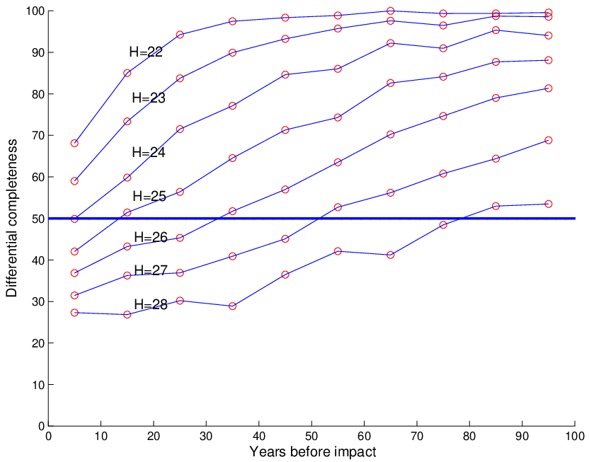
The main outcome of the simulation is shown in Fig. 4.

The left panel shows the differential discovery completeness as a function of time from the survey beginning and absolute magnitude. For each 10 yr bin, the differential discovery completeness is defined as the ratio between the number of impactors discovered and those impacting in that time frame. For example, the differential discovery completeness for $H=24$ and the bin from 20 to 30 yr is given by the fraction of objects discovered before the impact among those impacting between 20 and 30 yr with respect to the beginning of the survey operations.

For impactors with $H=23$ a 70% discovery completeness is achieved in the first decade, while the 90% threshold is reached after two more decades. For impactors with $H=25$ a 60% discovery completeness is achieved after two decades, while the 90% threshold is almost reached at the end of the simulation. For $H=28$ the discovery completeness starts slightly below 40%, and increases slowly during the next decades as expected, due to the small size of the objects. Notice that the completeness is greater than $50\%$ already from the start for $H=26$ .

The right panel shows the differential completeness for a lead time given by Eq. (1). This means that a discovery is considered successful only if it takes place sufficiently early, allowing the mitigation actions appropriate for the size of the impactor. For impactors with $H=23$ a $\simeq 60\%$ completeness is achieved in the first decade, while the 90% threshold is reached after 30 yr. For $H=25$ a $\simeq 50\%$ discovery completeness is achieved in the second decade, while the 90% threshold is not yet reached at the end of the simulation. For smaller asteroids the discovery completeness is larger than 25% from the beginning of the operations and overcomes the 50% threshold after more than 70 yr.

We can sum up the results in terms of blind time, that is the intersection between the 50% completeness and the $H=const$ curves in Fig. 4. The survey simulated in this paper would have a blind time of about 20 yr for imminent impactors with $H=25$ . Note that a Tunguska-sized ( $H\simeq 24.5$ ) object impacting within 10 yr from the start of the survey would have a $>60\%$ probability of being discovered and would have a lead time larger than 1 week with a probability $\simeq 45\%$ . For smaller impactors the blind time increases up to $\sim$ 60 yr for $H=28$ .

Figure 5 shows the distribution of the lead time for different values $H$ . As expected, the lead time strongly depends on the value of the absolute magnitude. A clear trimodality is visible in all the panels: either the object impacts without being discovered (left bar), or is discovered during its last apparition (central peak), or at a previous apparition (right peak). Table 1 details the fractions of objects in each peak for a fixed value of $H$ . Most of the impactors with $H=22$ are discovered during a previous apparition with respect to the impact. As $H$ increases there are more and more cases of objects either discovered during the last apparition or not discovered at all.

To conclude this discussion we report the integral completeness achieved by our simulated survey. The integral completeness is computed by the weighted sum

\text{Comp}(H\leq\bar{H})=\sum_{22\leq H_{i}\leq\bar{H}}w_{H_{i}}\text{Comp}(H_{i})\ \big/\sum_{22\leq H_{i}\leq\bar{H}}w_{H_{i}}

where $\text{Comp}(H)$ is the completeness for a fixed absolute magnitude $H$ . To get a more realistic result we keep into account a power law distribution for the number of asteroids at a given absolute magnitude. Consistently with Bottke et al. (2002) and Stuart and Binzel (2004), the computed efficiencies for a fixed absolute magnitude value $H$ are given the weights:

w_{H}=10^{0.37(H-28)}\,.

The results are summarized in Fig. 6.

$H$	undiscovered	last apparition	previous apparition
22	4.2%	8.9%	86.9%
23	8.1%	13.6%	78.4%
24	15.0%	18.5%	66.5%
25	22.3%	25.8%	51.9%
26	31.4%	31.0%	37.6%
27	41.3%	33.0%	25.7%
28	52.1%	31.1%	16.8%

Table 1: Percentages of impactors not discovered (2nd column), discovered during the last apparition (3rd column) or discovered at a previous apparition (4th column), as a function of

H

(1st column).

5 Conclusions

We simulated the operations, over a time span of 100 yr, of a Wide Survey capable of covering all the sky at solar elongation larger than $40^{\circ}$ , down to apparent magnitude 21.5, with a nightly cadence. The survey includes the operation of follow-up with a limiting magnitude 23.0.

The goal of the simulation was to compute the “blind time” of the survey, i.e., the time between the start of survey operations and the moment at which 50% of the impactors at a given magnitude are discovered and their orbits determined, with an advance large enough to allow undertaking the appropriate mitigation actions. In fact, our modeling allowed us to compute a realistic distribution of the lead time, i.e., the interval of time between the first orbit determination and the time of impact. The distribution shows a trimodality corresponding to 1) undiscovered objects, 2) objects discovered at the impact apparition, and 3) objects discovered during a previous apparition.

The survey discussed in this paper can efficiently deal with Tunguska-sized impactors for which the blind time is about 10 yr. This means that, already in the first ten years of survey operations, there would be 50% probability of discovering such an impactor at least one week before impact. The pre-impact discovery of Tunguska-sized impactors was not an original goal of past NEO surveys but the case of 2008TC3 and the present paper show that it is becoming within reach.

In a future paper, we plan to compare the performances of the discussed Wide Survey and a state of the art Deep Survey thus allowing us to quantitatively measure the contribution of the Wide Survey to the current NEO search programs.

Acknowledgements

This study was partly supported by ESA Contract n. 22929/09/ML/GLC and by the PRIN INAF “Near Earth Objects”. The authors wish to thank A. Milani for useful discussions during the development of this work, S. R. Chesley for providing us with the impactor population. We thank S. R. Chesley and an anonymous referee for their constructive comments.

Appendix A Impactor radiants

Following Valsecchi et al. (1999) it is possible to establish that in the framework of Öpik’s theory of close encounters (Öpik, 1976) the angles $\theta$ and $\phi$ define the direction opposite to that from which an Earth impactor seems to arrive (the so-called radiants in meteor astronomy). These angles can be computed from the orbital elements $a$ , $e$ , $i$ of the impactor ( $a$ must be given in units of the orbital semimajor axis of the planet, for Earth impactors in AU) as follows:

$\displaystyle\cos\theta$	$\displaystyle=$	$\displaystyle\frac{\sqrt{a(1-e^{2})}\cos{i}-1}{\sqrt{3-1/a-2\sqrt{a(1-e^{2})}\cos{i}}}$
$\displaystyle\sin\theta$	$\displaystyle=$	$\displaystyle\frac{\sqrt{2-1/a-a(1-e^{2})\cos^{2}{i}}}{\sqrt{3-1/a-2\sqrt{a(1-e^{2})}\cos{i}}}$
$\displaystyle\sin\phi$	$\displaystyle=$	$\displaystyle\pm\frac{\sqrt{2-1/a-a(1-e^{2})}}{\sqrt{2-1/a-a(1-e^{2})\cos^{2}{i}}}$
$\displaystyle\cos\phi$	$\displaystyle=$	$\displaystyle\pm\frac{\sqrt{a(1-e^{2})}\sin{i}}{\sqrt{2-1/a-a(1-e^{2})\cos^{2}{i}}},$

where in the expression for $\sin\phi$ the upper sign applies to collisions in the post-perihelion branch of the orbit, and in that for $\cos\phi$ to collisions at the ascending node.

$\sin\phi>0$	$\cos\phi>0$	$\omega+f=0$	$0<f<\pi$
$\sin\phi<0$	$\cos\phi>0$	$\omega+f=0$	$\pi<f<2\pi$
$\sin\phi>0$	$\cos\phi<0$	$\omega+f=\pi$	$0<f<\pi$
$\sin\phi<0$	$\cos\phi<0$	$\omega+f=\pi$	$\pi<f<2\pi$

Table 2: The relationship between the quadrant of

\phi

and the orbital elements

\omega

and

f

of the impactor at collision.

Thus, to each triple $a$ , $e$ , $i$ correspond four encounter geometries, all characterized by the same value of $\theta$ , that differ for the quadrant of $\phi$ ; this, in turn, can be computed from the orbital elements of the impactor, as shown in Table 2.

Meteor radiants are often plotted using an equal area projection centered on the direction of the Earth motion, with the ecliptic as reference plane; in this case, starting from $\theta$ and $\phi$ computed from the meteoroid orbits, the radiant coordinates are simply given by $\lambda+\pi$ and $-\beta$ ( $\beta=0$ defines the ecliptic plane, and $\lambda=\beta=0$ is the direction of the Earth motion), with $\lambda$ and $\beta$ given by

\sin\beta=\sin\theta\cos\phi\ \ ,\ \ \sin\lambda=\frac{\sin\theta\sin\phi}{\cos\beta}\ \ ,\ \ \cos\lambda=\frac{\cos\theta}{\cos\beta}.

For an asteroidal Earth impactor, it is useful to use the same representation, but in this case centered on the opposition point, something that is obtained by rotating $\lambda$ by $\pi/2$ in the appropriate direction.

A.1 An analytical expression

The non-uniform sky distribution shown in Fig. 3 can be exploited in prioritizing the sky coverage for a survey aimed at detecting very close Earth approachers and impactors.

In this respect, an important quantity to take into account is the angular distance of the radiant from the Sun, that we will denote with $\sigma$ , since with ground based optical telescopes it is practically impossible to observe at values of this quantity smaller than some practical limit. Thus, in order to evaluate the efficiency of an impactor-aimed sky survey, it is important to establish what fraction of impactor radiants lies below this angular distance from the Sun; to this purpose, it is necessary to discuss the geometric setup of Öpik’s theory Valsecchi et al. (1999).

We use a reference frame centered on the Earth, with the $z$ -axis perpendicular to the plane of the ecliptic, the $y$ -axis in the direction of the Earth velocity and the $x$ -axis pointing away from the Sun, which is located at $x=-1$ , $y=0$ , $z=0$ ; in this frame, the unperturbed geocentric encounter velocity $\vec{U}$ of the NEO has components

(U_{x},U_{y},U_{z})=(U\sin\theta\sin\phi,U\cos\theta,U\sin\theta\cos\phi)

where $U$ is the magnitude of the velocity vector. With these definitions, the cosine of the angle between $\vec{U}$ and the $x$ -axis is simply given by $\sin\theta\sin\phi$ ; this angle, in turn, is equal to $\pi-\sigma$ since, as noted before, $\theta$ and $\phi$ define the direction opposite to the radiant.

Thus, if $\sigma_{min}$ is the minimum angular distance from the Sun that the survey can reach, the radiants that are not observable by it are characterized by

\cos\sigma_{min}<\sin\theta\sin\phi.

Since for each triple $a$ , $e$ , $i$ we have four possible associated radiants, two of which with $\sin\phi>0$ and the other two with $\sin\phi<0$ , the consequence of the above inequality is that for $\sigma_{min}<\pi/2$ we have the following two cases:

1.

for $|\cos\sigma_{min}|\geq|\sin\theta\sin\phi|$ , all four radiants associated to a given triple $a$ , $e$ , $i$ are observable;
2.

for $|\cos\sigma_{min}|<|\sin\theta\sin\phi|$ , the two radiants for which $\sin\phi<0$ are observable, while the other two are not.

Given a population of impactors, it is then possible to compute the fraction $F$ of radiants that have $\sigma>\sigma_{min}$ ; if $h$ is the fraction of the population characterized by $|\cos\sigma_{min}|\geq|\sin\theta\sin\phi|$ , then

F=h+\frac{1-h}{2}=\frac{1+h}{2}.

References

Bottke et al. (2002) Bottke, W. F., Morbidelli, A., Jedicke, R., Petit, J.-M., Levison, H. F., Michel, P., Metcalfe, T. S. 2002. Debiased Orbital and Absolute Magnitude Distribution of the Near-Earth Objects. Icarus 156, 399-433.
Brown et al. (2002) Brown, P., Spalding, R. E., ReVelle, D. O., Tagliaferri, E., Worden, S. P. 2002. The flux of small near-Earth objects colliding with the Earth. Nature 420, 294-296.
Chesley and Spahr (2004) Chesley, S. R., Spahr, T. B. 2004. Earth impactors: orbital characteristics and warning times. Mitigation of Hazardous Comets and Asteroids, Eds. M. J. S. Belton et al., Cambridge University Press, 22-37.
Cibin et al. (2011) Cibin, L. et al. 2011. A dynamic observation concept as a key point for an enhanced SSA optical network. Proceedings of the European Space Surveillance Conference WPP-321, 7-9 June 2011, Madrid, Spain.
Farnocchia et al. (2011) Farnocchia, D., Bernardi, F., Milani, A. 2011. The performances of a wide survey on a population of impactors. Proceedings of the IAA Planetary Defense Conference, Bucharest, Romania.
Hills and Leonard (1995) Hills, J. G., Leonard, P. J. T. 1995. Earth-crossing asteroids: The last days before earth impact. The Astronomical Journal 109, 401-417.
Mainzer et al. (2011) Mainzer, A., et al. 2011. NEOWISE Observations of Near-Earth Objects: Preliminary Results. The Astrophysical Journal 743, 2.
Milani et al. (2004) Milani, A., Gronchi, G. F., Vitturi, M. D., Knežević, Z. 2004. Orbit determination with very short arcs. I admissible regions. Celestial Mechanics and Dynamical Astronomy 90, 57-85.
Milani et al. (2005) Milani, A., Chesley, S. R., Sansaturio, M. E., Tommei, G., Valsecchi, G. B. 2005. Nonlinear impact monitoring: line of variation searches for impactors. Icarus 173, 362-384.
Milani et al. (2007) Milani, A., Gronchi, G. F., Knežević, Z. 2007. New Definition of Discovery for Solar System Objects. Earth Moon and Planets 100, 83-116.
Milani and Gronchi (2010) Milani, A., Gronchi, G. F. 2010. Theory of Orbital Determination. Theory of Orbital Determination, by Andrea Milani and Giovanni F. Gronchi. ISBN 978-0-521-87389-5. Published by Cambridge University Press, Cambridge, UK, 2010. .
Milani et al. (2012) Milani, A., et al. 2012. Identification of known objects in solar system surveys. ArXiv e-prints arXiv:1201.2587.
Morrison (1992) Morrison, D. 1992. The Spaceguard Survey: Report of the NASA International Near-Earth-Object Detection Workshop. NASA STI/Recon Technical Report N 92, 34245.
Öpik (1976) Öpik, E. J. 1976. Interplanetary encounters - Close-range gravitational interactions. Developments in Solar System- and Space Science, Amsterdam: Elsevier, 1976 .
Stokes et al. (2002) Stokes, G. H., Evans, J. B., Larson, S. M. 2002. Near-Earth Asteroid Search Programs. Asteroids III 45-54.
Stuart and Binzel (2004) Stuart, J. S., Binzel, R. P. 2004. Bias-corrected population, size distribution, and impact hazard for the near-Earth objects. Icarus 170, 295-311.
Tonry (2011) Tonry, J. L. 2011. An Early Warning System for Asteroid Impact. Publications of the Astronomical Society of the Pacific 123, 58-73.
Valsecchi et al. (1999) Valsecchi, G. B., Jopek, T. J., Froeschle, C. 1999. Meteoroid stream identification: a new approach - I. Theory. Monthly Notices of the Royal Astronomical Society 304, 743-750.
Vereš et al. (2009) Vereš, P., et al. 2009. Detection of Earth-impacting asteroids with the next generation all-sky surveys. Icarus 203, 472-485.