GTRACE-RS: Efficient Graph Sequence Mining
using Reverse Search

Graph mining is the task of finding novel, useful, and “understandable” graph-theoretic patterns in a graph representation of data [5]. Frequent graph mining is a representative task in graph mining that efficiently mines all subgraphs that appear more frequently than a given threshold from a set of labeled graphs.

A graph database $DB$ is a set of tuples $\langle gid,g\rangle$, where $gid$ is a graph ID and $g$ is a labeled graph. A tuple $\langle gid,g\rangle$ is said to contain a graph $p$, if $p$ is a subgraph of $g$, i.e., $p\sqsubseteq g$. The support of graph $p$ in database $DB$ is the number of tuples in the database containing $p$, i.e., $\sigma(p)=|\{gid\mid(\langle gid,g\rangle\in DB)\wedge(p\sqsubseteq g)\}|.$ Given a positive integer $\sigma^{\prime}$ as the support threshold, a graph $p$ is called a “frequent subgraph” pattern in the graph database $DB$, if at least $\sigma^{\prime}$ tuples in the database contain $p$, i.e., $\sigma(p)\geq\sigma^{\prime}$. Representative methods for frequent graph mining, such as AGM [10], gSpan [19], and Gaston [16], mine frequent subgraphs starting with those of size 1, using the anti-monotonicity of the support values.

We briefly review gSpan, because it is used to implement the method proposed in this paper. Here, for the sake of simplicity, we assume that edges in graphs have labels, whereas vertices in the graphs do not. Given a frequent pattern $p$ with $n$ vertices and $k$ edges, vertices in $p$ are traversed in a depth first manner to assign vertex IDs from $v_{1}$ to $v_{n}$. The starting vertex and the last visited vertex in the traversal are called the root $v_{1}$ and the rightmost vertex $v_{n}$, respectively, while the straight path from $v_{1}$ to $v_{n}$ is called the rightmost path. According to the traversal, $p$ is represented by DFS code consisting of triplets $(u,u^{\prime},l)$, where $l$ is an edge label between vertices $v_{u}$ and $v_{u^{\prime}}~(1\leq u,u^{\prime}\leq n)$. The linear order of the DFS codes is defined as follows. For DFS codes $\alpha=(a_{1},a_{2},\cdots,a_{k})$ and $\beta=(b_{1},b_{2},\cdots,b_{h})$, $\alpha\preceq\beta$, iff either of the following conditions is true:

• •

  $\exists t,1\leq t\leq min(k,h),a_{q}=b_{q}~for~q<t,a_{t}\prec_{e}b_{t}$

• •

  $a_{q}=b_{q}~for~0\leq q\leq k,~and~k\leq h$

where $\prec_{e}$ is the linear order among the triplets $(u,u^{\prime},l)$. Since there are many DFS codes for an identical $p$, the minimal DFS code of the DFS codes representing $p$ is defined as the canonical code for $p$.

A frequent subgraph $p$ is extended based on the pattern-growth principle. Given a DFS code $\alpha=(a_{1},a_{2},\cdots,a_{k})$ for $p$ with $k$ edges, $p$ is extended by adding a new edge to obtain a new pattern with $k+1$ edges, which is represented by $\alpha^{\prime}=(a_{1},a_{2},\cdots,a_{k},a_{k+1})$. The new edge can be added between the rightmost vertex and other vertices on the rightmost path (backward extension), or it can introduce a new vertex and connect to vertices on the rightmost path (forward extension). Overall, new edges are only added to the vertices along the rightmost path. With this restricted extension, gSpan reduces the generation of the same frequent subgraphs. However, it still guarantees the completeness of enumerating all frequent subgraphs.

In this section, we briefly review the compilation used to represent graph sequences compactly in GTRACE. Figure 1(a) shows an example of a graph sequence. Graph $g^{(j)}$ is the $j$-th labeled graph in the sequence. The problem we address in this paper is how to mine patterns that appear more frequently than a given threshold from a set of graph sequences. In [11], Inokuchi and Washio proposed TRs to represent graph sequences compactly under the assumption that “the change over successive graphs is gradual”. In other words, only a small part of the graph changes between two successive graphs $g^{(j)}$ and $g^{(j+1)}$ in a graph sequence, while the other parts remain unchanged. In the aforementioned human and gene networks, this assumption certainly holds, because most of the changes in vertices are progressive over successive steps. A direct representation of a graph sequence is not compact, because many parts of the graph remain unchanged over several steps and are therefore redundant in the representation. On the other hand, a graph sequence can be compactly represented by introducing a representation of graph transformation based on rules for insertion, deletion, and relabeling of vertices and edges under the gradual change assumption.

A labeled graph $g$ is represented as $g=(V,E,L,f)$, where $V=\{v_{1},\cdots,v_{z}\}$ is a set of vertices, $E=\{(v,v^{\prime})\mid(v,v^{\prime})\in V\times V\}$ is a set of edges, and $L$ is a set of labels such that $f:V\cup E\rightarrow L$. A graph sequence is represented as $d=\langle g^{(1)}~g^{(2)}\cdots g^{(n)}\rangle$. We assume that each vertex $v$ is mutually distinct from the others in $g^{(j)}$ and has a vertex ID $id(v)$ in $d$. We define the set of vertex IDs to be $ID_{V}(d)=\{id(v)\mid v\in V(g^{(j)}),g^{(j)}\in d\}$ and the set of pairs of vertex IDs to be $ID_{E}(d)=\{(id(v),id(v^{\prime}))\mid(v,v^{\prime})\in E(g^{(j)}),g^{(j)}\in d\}$. For example, in the human network mentioned in Section 1, each person has a vertex ID, and his/her gender is an example of a vertex label. To represent a graph sequence compactly, we focus on the differences between two successive graphs $g^{(j)}$ and $g^{(j+1)}$ in the sequence.

We call $g^{(j)}$ and $g^{(j,k)}$ an interstate and intrastate, respectively. The order of interstates represents the order of graphs in a sequence. On the other hand, the order of intrastates is the order of graphs in the artificial interpolation.

The transformation is represented by the following TR.

For the sake of simplicity, we denote the TR $tr^{(j,k)}_{[o_{jk},l_{jk}]}$ as $tr^{(j,k)}_{[o,l]}$ by omitting the subscripts for $o_{jk}$ and $l_{jk}$, except where this is likely to cause ambiguity. In [11], Inokuchi and Washio introduced six TRs as defined in Table 2. In summary, we give the following definition of a transformation sequence.

The notion of an interstate transformation sequence is far more compact than the original graph based representation, because only the differences between two successive interstates appear in the sequence. In addition, in our case, computing a sequence of TRs based on differences between two graphs is solvable in linear time because all vertices have vertex IDs.

In this section, we briefly review how GTRACE mines rFTSs (relevant frequent transformation subsequences) from a given set of graph sequences. To mine rFTSs from a set of transformation sequences, we define an inclusion relation between transformation sequences.

The first condition in Definition 4 states that $\phi$ preserves the order among intrastate transformation sequences, while the second condition states an injective mapping from vertex IDs in $s_{p}$ to vertex IDs in $s_{d}$. In addition, the third condition states that a TR corresponding to any TR in $s_{p}$ must exist in $s_{d}$. The complexity of finding an occurrence of $s_{p}$ in $s_{d}$ is identical to that of subgraph isomorphism matching.

To mine FTSs consisting of mutually relevant vertices only, the relevancy of vertices and edges is defined as follows²² 2 See [11, 12] for the detail motivations for mining rFTSs..

Similar to Definition 5, we define the union graph of the transformation sequence $s_{d}$.

Given a set of data $DB=\{\langle gid,d\rangle\mid d=\langle g^{(1)}~\cdots~g^{(n)}\rangle\}$, the support value $\sigma(s_{p})$ of a transformation subsequence $s_{p}$ is given as

where $s_{d}$ is the transformation sequence of $d$. We call a transformation subsequence with support value greater than or equal to a minimum support threshold $\sigma^{\prime}$ a “frequent transformation subsequence” (FTS). The anti-monotonicity of this support value holds; that is, if $s_{1}\sqsubset s_{2}$ then $\sigma(s_{1})\geq\sigma(s_{2})$. Using these definitions, we state our mining problem as follows.

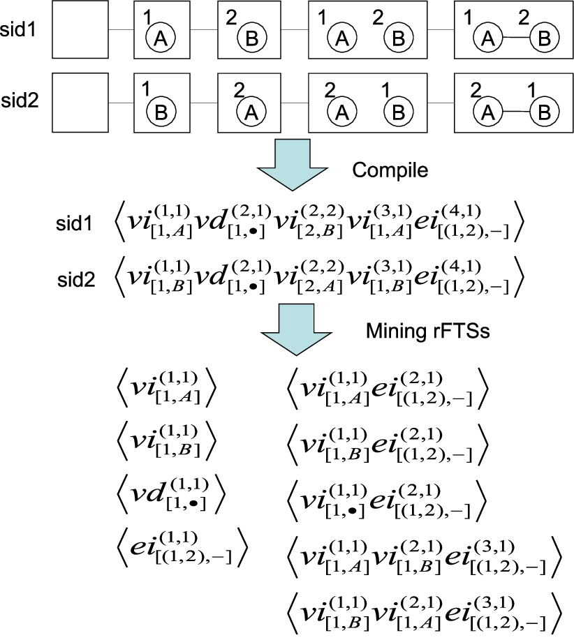
To enumerate all rFTSs efficiently, GTRACE recursively mines FTSs by appending a TR to the tail of the current FTS, in a similar manner to PrefixSpan [17], which is a representative method for mining frequent subsequences from a set of itemset sequences. After mining all the FTSs, GTRACE removes all FTSs whose union graphs are not connected, thus outputting only rFTSs.

In the previous subsection, we briefly reviewed the problem of graph sequence mining and GTRACE for mining rFTSs from graph sequences. GTRACE first mines a set of FTSs containing a complete set of rFTSs, and then removes any FTS that is not relevant from the set of mined FTSs during post-processing. Since most of the FTSs mined in the first step are not rFTSs, excessive computation time is needed to mine the vast set of FTSs, causing GTRACE to be highly inefficient.

For example, the FTS $s_{6}$ shown in Fig. 8 is relevant, because its union graph is connected. To mine this rFTS, GTRACE mines $s_{1}$, $s_{2}$, $s_{3}$, $s_{4}$, and $s_{5}$ in order appending a TR to the tail of $s_{i}$ to obtain a new FTS $s_{i+1}$, where $i=2,\cdots,5$. Then, $s_{2}$, $s_{3}$, and $s_{4}$ are removed during post-processing, because they are irrelevant. Therefore, to mine all rFTSs using GTRACE, a vast set of FTSs, most of which are not rFTSs, first needs to be mined, resulting in inefficient execution of GTRACE. In our experiment, 95% of FTSs mined by GTRACE are irrelevant. By designing a new algorithm that mines only rFTSs, we can reduce the computation time for mining the complete set of rFTSs. In the next section, we propose a new method for mining only rFTSs from a set of graph sequences based on the principle of a reverse search.

To mine all rFTSs efficiently, we propose a method for mining only rFTSs based on a reverse search [2, 1]. The underlying concept of the reverse search is a general scheme for designing efficient algorithms for hard enumeration problems. Let $S$ be the set of solutions. In a reverse search, we define the parent-child relation $P\in S\times S$ such that each $x\in S$ has a unique parent $P(x)\in S$. Using the search tree $T$ over $S$ defined by $P$, we can enumerate all solutions of $S$ without duplicates by traversing the search tree $T$ from the root to the leaves. Therefore, if we can define the parent-child relation $P$ such that each $x\in S$ has a “unique” parent, we can enumerate a complete set of elements in $S$.

For example, given a set of items $I=\{i_{1},\cdots,i_{|I|}\}$ and a set of transactions $D=\{t\mid t\subseteq I\}$, the frequent itemset mining problem is to enumerate all frequent itemsets $S=\{x\mid x\subseteq I,\sigma(x)\geq\sigma^{\prime},~\sigma(x)=|\{t\mid x\subseteq t,t\in D\}|\}$, where $\sigma^{\prime}$ is the minimum support threshold. To enumerate the complete set of frequent itemsets efficiently, the parent-child relation $P$ is defined as the unique itemset $x^{\prime}=\{i_{1},i_{2},\cdots,i_{k-1}\}$ derived from $x=\{i_{1},i_{2},\cdots,i_{k-1},i_{k}\}$ by removing the last item $i_{k}$ in $x$, where the items in $x$ and $x^{\prime}$ are sorted according to the linear order of the items. Starting from the root node corresponding to an empty set, traversing the search tree $T$ over $S$ defined by $P$ enables us to enumerate a complete set of frequent itemsets without duplicates. In the traversal, $P^{-1}(x^{\prime})$ is used to enumerate itemsets from itemset $x^{\prime}\in S$ by adding an item to $x^{\prime}$. Figure 9 shows the enumeration tree for the itemset $I=\{A,B,C,D\}$, with $2^{I}$ nodes in the tree. By traversing from the root node in a reverse direction to the arrows in the tree, all itemsets are enumerated.

However, as mentioned in Section 2.3, if the last TR in an rFTS $s_{i}~(i=2,\cdots,6)$ is removed to derive its parent FTS $s_{i-1}$, $s_{i-1}$ is not always relevant, although $s_{i-1}$ is always frequent according to the anti-monotonicity of the support values. Therefore, the original GTRACE needs all the FTSs to enumerate all the rFTSs, which results in inefficient execution of GTRACE. In this section, to enumerate only rFTSs, we define canonical forms of rFTSs and novel parent-child relations $P_{1}$, $P_{2}$, and $P_{3}$ between the canonical rFTSs.

In Definition 7, $P_{1}$, $P_{2}$, and $P_{3}$ are parent-child relations among canonical rFTSs $S$, which are defined as follows.

If the length of transformation sequence $s$ is defined as the number of TRs in $s$, the following lemma is obtained.

According to Lemma 1, $P_{1}(s)$ is always relevant for an rFTS $s$ containing TRs applied to vertices. In addition, the transformation sequence $P_{1}(s)$ is frequent according to the anti-monotonicity of the support value and canonical according to Definition 7. Therefore, $P_{1}(s)$ returns a “unique” rFTS in $S$.

Next, we define the second function of our parent-child relation to enumerate rFTSs.

If the rFTS $s$ contains TRs that are applied to vertices, we can obtain an rFTS $s^{\prime}$ that does not contain TRs applied to vertices by applying $P_{1}$ to $s$ multiple times. In addition, $P_{2}$ is applicable to $s^{\prime}$, if the length of $s^{\prime}$ is greater than the number of edges in $g_{u}(s^{\prime})$, since at least one TR needs to be applied to each edge in $E(g_{u}(s^{\prime}))$. According to the above definition, the following lemma is obtained.

This lemma is proven in the same way as Lemma 1. According to Lemma 2, $P_{2}(s^{\prime})$ is always relevant for an rFTS $s^{\prime}$ containing only TRs applied to edges. In addition, the transformation sequence $P_{2}(s^{\prime})$ is frequent according to the anti-monotonicity of the support value and canonical according to Definition 7. Therefore, $P_{2}(s^{\prime})$ returns a “unique” rFTS in $S$.

Finally, we define the third function of our parent-child relation to enumerate rFTSs.

If each TR in an rFTS $s$ is not applied to a mutually different edge in $g_{u}(s)$, we can obtain an rFTS $s^{\prime\prime}$ where each TR is applied to a mutually different edge in $g_{u}(s^{\prime\prime})$ by applying $P_{1}$ and $P_{2}$ to $s$ multiple times. According to Definition 10, $P_{3}(s^{\prime\prime})$ is always relevant for an rFTS $s^{\prime\prime}$ where each TR is applied to a mutually different edge in $g_{u}(s^{\prime\prime})$, because the connectivity of $g_{u}(P_{3}(s^{\prime\prime}))$ is kept. In addition, the transformation sequence $P_{3}(s^{\prime\prime})$ is frequent according to the anti-monotonicity of the support value and canonical according to Definition 7. Therefore, $P_{3}(s^{\prime\prime})$ returns a “unique” rFTS in $S$.

We have defined our parent-child relation between rFTSs in terms of three functions $P_{1}$, $P_{2}$, and $P_{3}$. Using the search tree $T$ over $S$ defined by $P=\{P_{1},P_{2},P_{3}\}$, we can enumerate a complete set of only rFTSs of $S$ by traversing search tree $T$ from its root. In the traversal, $P_{1}^{-1}$, $P_{2}^{-1}$, and $P_{3}^{-1}$ are used to enumerate rFTSs from the current rFTS by adding a TR.

In the previous subsection, we defined functions $P_{1}$, $P_{2}$, and $P_{3}$ for the parent-child relation between rFTSs. By traversing the tree constructed by parent-child relations in a reverse direction, we enumerate a complete set of rFTSs without enumerating any FTSs that are not also rFTSs. Figure 11 gives the pseudo code for the proposed method “GTRACE-RS” that mines all rFTSs from graph sequences $DB$ and accumulates them in $S$ with the minimum support value $\sigma^{\prime}$. The method traverses the search tree $T$ over $S$ defined by $P=\{P_{1},P_{2},P_{3}\}$ in a depth-first manner. In Fig. 11, $s_{p}\Diamond r$ means that a TR $r$ is added to $s_{p}$ such that $s_{p}\Diamond r\in P^{-1}_{i}(s_{p})$, where $i=1,2,3$. In this process, a TR to be added is not always appended to the tail of $s_{p}$ unlike the original GTRACE. $s_{p}\neq$ min checks whether $s_{p}$ has been discovered before, where min is the canonical form of $s_{p}$. First, given an rFTS $s_{p}$ that contains only TRs applied to edges and where each TR is applied to a mutually different edge in $g_{u}(s_{p})$, GTRACE-RS enumerates rFTSs that are $P_{3}^{-1}(s_{p})$. Next, given an rFTS that contains only TRs applied to edges, GTRACE-RS enumerates rFTSs that are $P_{2}^{-1}(s_{p})$. Finally, given an rFTS, GTRACE-RS enumerates rFTSs that are $P_{1}^{-1}(s_{p})$.

References

- [1] T. Asai, et. al. Efficient Tree Mining Using Reverse Search. Technical Report 218, Department of Informatics, Kyushu University, (2003)
- [2] D. Avis and K. Fukuda. Reverse Search for Enumeration. Discrete Applied Mathematics, Vol. 65, pp. 21–46, (1996).
- [3] M. Berlingerio, et. al. Mining Graph Evolution Rules. Proc. of Euro. Conf. on Principles and Practice of Knowledge Discovery in Databases (PKDD), pp. 115–130. (2009)
- [4] K. Borgwardt, et. al. Pattern Mining in Frequent Dynamic Subgraphs. Proc. of Int’l Conf. on Data Mining (ICDM), pp. 818–822. (2006)
- [5] D. Cook, et. al. Graph-based Mining of Complex Data. Advanced Methods for Knowledge Discovery from Complex Data, pp. 75–93. (2005)
- [6] D. Cook and L. Holder. Mining Graph Data. Wiley-Interscience, (2006)
- [7]
Enron Email Dataset,
http://www.cs.cmu.edu/~enron/ - [8] M. Fiedler and C. Borgelt. Subgraph Support in a Single Large Graph. Proc. of Workshop on Mining Graphs and Complex Structures (MGCS), pp. 399–404. (2007)
- [9] M. Garey and D. Johnson. Computers and Intractability: A Guide to Theory of NP-Completeness, W.H. Freeman. (1979)
- [10] A. Inokuchi, et. al. An Apriori-based Algorithm for Mining Frequent Substructures from Graph Data. Proc. of Euro. Conf. on Principles of Data Mining and Knowledge Discovery (PKDD), pp. 13–23. (2000)
- [11] A. Inokuchi and T. Washio. A Fast Method to Mine Frequent Subsequences from Graph Sequence Data. Proc. of Int’l Conf. on Data Mining (ICDM), pp. 303-312. (2008)
- [12] A. Inokuchi and T. Washio. Mining Frequent Graph Sequence Patterns Induced by Vertices. Proc. of SIAM Int’l Conf. on Data Mining (SDM), pp. 466-477. (2010)
- [13] B. Klimt and Y. Yang. Introducing the Enron Corpus. Proc. of Conf. on Collaboration, Electronic messaging, Anti-Abuse and Spam (CEAS), (2004)
- [14] M. Kuramochi and G. Karypis. Frequent Subgraph Discovery. Proc. of Int’l Conf. on Data Mining (ICDM), pp. 313-320. (2001)
- [15] M. Kuramochi and G. Karypis. Finding Frequent Patterns in a Large Sparse Graph. Proc. of SIAM Int’l Conf. on Data Mining (SDM), (2004)
- [16] S. Nijssen and J. Kok. A Quickstart in Frequent Structure Mining can Make a Difference. Proc. of Int’l Conf. on Knowledge Discovery and Data Mining (KDD), pp. 647–652. (2004)
- [17] J. Pei, et. al. PrefixSpan: Mining Sequential Patterns by Prefix-Projected Growth, Proc. of Int’l Conf. on Data Engineering (ICDE), pp. 2–6. (2001)
- [18] A. Sanfeliu and K. Fu. A Distance Measure Between Attributed Relational Graphs for Pattern Recognition, IEEE Transactions on Systems, Man and Cybernetic, Vol. 13, pp. 353–362. (1983)
- [19] X. Yan and J. Han. gSpan: Graph-Based Substructure Pattern Mining. Proc. of Int’l Conf. on Data Mining (ICDM), pp. 721–724. (2002)