August 24, 2026
Lectures on holographic non-Fermi liquids and quantum phase transitions
Abstract
In these lecture notes we review some recent attempts at searching for non-Fermi liquids and novel quantum phase transitions in holographic systems using gauge/gravity duality. We do this by studying the simplest finite density system arising from the duality, obtained by turning on a nonzero chemical potential for a global symmetry of a CFT, and described on the gravity side by a charged black hole. We address the following questions of such a finite density system:
- 1.
Does the system have a Fermi surface?
What are the properties of low energy excitations near the Fermi surface? - 2.
Does the system have an instability to condensation of scalar operators?
What is the critical behavior near the corresponding quantum critical point?
We find interesting parallels with those of high cuprates and heavy electron systems. Playing a crucial role in our discussion is a universal intermediate-energy phase, called a “semi-local quantum liquid,” which underlies the non-Fermi liquid and novel quantum critical behavior of a system. It also provides a novel mechanism for the emergence of lower energy states such as a Fermi liquid or a superconductor.
Lectures by HL at TASI 2010, Boulder, June 2010; KITPC workshop/school on “AdS/CM duality and other approaches,” Beijing, November, 2011; School on “Holographic View of Condensed Matter Physics” at International Institute of Physics, the Federal University of Rio Grande do Norte, Natal, Brazil, July 2011.
I Introduction and motivation
Understanding phases of matter for which there is no quasiparticle description presents some of the most challenging problems in physics. Examples include the quark-gluon plasma (QGP) created in heavy ion collisions at RHIC during the past decade and now at LHC and ultracold atomic systems at unitarity. In condensed matter physics prominent examples include the quantum spin liquid phase of a magnetic insulator, the “strange metals” occurring in the normal state of the high temperature cuprate superconductors, and heavy electron systems near a quantum phase transition. There has been an accumulation of examples, but so far no satisfactory theoretical framework exists to describe them. Finding solvable examples of quantum phases with no quasiparticles should provide a valuable guide for the search for such a framework.
During the last decade, developments in string theory have revealed surprising and profound connections between gravity and many-body systems. The so-called gauge/gravity duality (or AdS/CFT, or holographic duality), relates a classical gravity theory in a weakly curved -dimensional anti-de Sitter (AdSd+1) spacetime to a strongly-coupled -dimensional quantum field theory living on its boundary [1, 3, 2]. This suggests that complicated questions in strongly interacting many-body physics can be mapped to simple problems in classical gravity, i.e. to geometry, potentially giving rise to a new paradigm for approaching many-body dynamics. In particular, black holes appear to play a universal role in characterizing quantum phases without quasiparticles, giving important insight into dynamical behavior of such systems.
Black holes are known for their simplicity and universality; assuming rotational symmetry, the geometry of a black hole is fully specified by its mass and certain conserved charges such as electric charge, independent of other details of a gravity system (such as matter content). Moreover, for a given mass, there is a maximal allowed charge. A quark-gluon plasma has almost equal number of “quarks” and “anti-quarks” and the temperature is the main characteristic energy scale. Such a state is described on the gravity side by a black hole of almost zero charge, i.e. a Schwarzschild black hole. In contrast, systems which are of interest in condensed matter physics, like strange metals, are finite density systems, with temperature much smaller than the chemical potential (a strange metal has only electrons but no positrons!). On the gravity side these finite density systems are described by black holes having close to the maximum charges. Thus, in some sense black holes provide a unified description of such seemingly distant systems like a QGP and a strange metal.
Using gravity dual to explore dynamical properties of holographic QGPs has provided important insights into the understanding of the QGP at RHIC (see e.g. [4, 5] and references therein). The goal of these notes is to bring these holographic tools to bear on strongly correlated systems at finite density. In particular, we review recent progress in finding new universal classes of non-Fermi liquids and novel quantum phase transitions using this approach.
I.1 Challenge: non-Fermi liquids
One of the cornerstones of condensed matter physics is Landau’s Fermi liquid theory, which underlies our understanding of almost all metals, semi-conductors, superconductors and superfluids. Since 1980’s there has been an accumulation of metallic materials whose thermodynamic and transport properties differ significantly from those predicted by Fermi liquid theory. These so-called non-Fermi liquids, which include the strange metal phase of cuprate superconductors and heavy fermion materials near a quantum phase transition, present important theoretical challenges. Here we first highlight some salient aspects of the Fermi liquid theory and then point out where it breaks down.
Let us start by recalling the story for a non-interacting Fermi gas (e.g. a gas of electrons in a box) for which the many-particle states can be obtained by simply filing single-particle energy eigenstates following the Pauli exclusion principle. The ground state is then given by filling all the (single-particle) states inside a sphere11 1 In these lectures we will only consider rotationally invariant theories, hence we will not encounter Fermi surfaces with shapes other than the sphere. in momentum space with radius determined by the density of fermions and with all states outside the sphere empty. The locus of points in momentum space at the boundary of this sphere, , is called the Fermi surface. The low-energy excitations of the system are given by either filling a state slightly outside the Fermi surface or removing a fermion from a filled state slightly inside the Fermi surface, and are called a particle and hole respectively. These excitations are gapless and have a linear dispersion (for ):
| (1) |
where denotes the free particle energy and we are working in the grand canonical ensemble, in which the energy of a excitation is measured from the chemical potential . Particles and holes22 2 Note that while all excitations have positive energies, it is convenient to represent a hole using negative energy, i.e. in terms of a filled particle state. are distinguished by the sign of . At a field theoretical level, these excitations manifest themselves as poles in the complex frequency plane of the retarded Green’s function for the electron operator in momentum space
| (2) |
where is again measured with respect to the chemical potential . Note that the retarded function is relevant as it describes the causal response of the system if we “add” an electron to the system. Fourier transforming (2) back in time we see that the propagator describes the propagation of a particle of energy :
| (3) |
which is of course as it should be for a free theory.
The situation becomes complicated once we switch on interactions between fermions, since the notion of single-particle states no longer makes sense. While one may intuitively expect that the qualitative picture for a non-interacting gas should still apply for sufficiently weak interactions, it is a priori not clear what should happen at finite or strong couplings. Landau’s Fermi liquid theory postulates that the above qualitative picture for a non-interacting gas in fact persists for generic interacting fermionic systems. In particular, it assumes that
- 1.
The ground state of an interacting fermionic system is characterized by a Fermi surface in momentum space at .
- 2.
Despite (possibly strong) interactions among fundamental fermions, the low energy excitations near the Fermi surface nevertheless behave like weakly interacting particles and holes, which are called quasi-particles and quasi-holes. They have the same charge as fundamental fermions and satisfy Fermi statistics. The dispersion of a quasi-particle (similarly for a quasi-hole) resembles (1) in free theory
(4) where can be considered as the effective mass of the quasi-particle and is in general different from the original fermion mass , from renormalization by many-body interactions.
Given the existence of a Fermi surface, the second postulate above is self-consistent. When turning on interactions, a particle (or hole) can now decay into another particle plus a number of particle-hole pairs. But it is not difficult to check that the exclusion principle constrains the phase space around a Fermi surface so much, that given generic local interactions among particles and holes, the decay (or scattering) rate of a particle (or hole) obeys
| (5) |
where is the energy of a particle (or hole). Thus, despite potentially strong interactions, particle or hole excitations near the Fermi surface have a long lifetime and an approximate particle picture still applies. (Below for simplicity we will refer to quasi-particles and quasi-holes collectively as quasi-particles.) Thus for a Fermi liquid, equation (3) should be modified to
| (6) |
which implies that near the Fermi surface the retarded function for the electron operator should have the form
| (7) |
with the self-energy
| (8) |
The residue of the pole, which is called the quasiparticle weight, can be interpreted as the overlap between the (approximate) one-quasiparticle state with the state generated by acting the electron operator on the vacuum.
The concept of quasi-particles is extremely powerful and makes it possible to develop a general low energy theory – Fermi liquid theory – independently of the precise microscopic details of a system. With some phenomenological input, the theory can then be used to predict essentially all the low energy behavior of the system. For example, the theory predicts that the specific heat is linear in temperature (see e.g. [6])
| (9) |
and that the low temperature resistivity increases with temperature quadratically
| (10) |
The theory has been tremendously successful in explaining almost all metallic states in nature.
It is important to emphasize that Fermi liquid theory does not require interactions among the fundamental constituents to be weak. For example for , one finds that , indicating that interactions among atoms are clearly not weak. There also exist so-called heavy electron compounds for which the effective mass for electron quasi-particles can be as large as times of the electron mass.
It is rather remarkable that weakly interacting quasiparticles can emerge as the low energy collective excitations of a strongly interacting many-body system, with only certain parameters (such as the effective mass) renormalized compared to the fundamental constituents of the system. The self-consistency of Fermi liquid theory can also be understood from an effective field theory perspective using the renormalization group [7, 8, 9]. Assuming the existence of quasi-particles, one can then try to write down the most general local effective field theory for them. One finds that due to kinematical constraints from the Fermi surface all interactions are irrelevant at low energies except for the forward scatterings33 3 The forward scatterings give rise to interactions among quasi-particles via their densities, which are incorporated in the Fermi liquid theory. Note that such interactions do not give rise to widths. and BCS-type pairing instabilities leading to a superconductor. Note that while the renormalization group analysis shows that the Fermi liquid theory is a stable fixed point (up to superconducting instabilities), it does not tell us whether or why a specific microscopic theory will flow to this fixed point.


Even though the Fermi liquid theory has been tremendously successful, nature always has interesting surprises for us. Since the 1980’s, there has been an accumulation of metallic materials whose thermodynamic and transport properties differ significantly from those predicted by Fermi liquid theory (see e.g. [10]). One prominent class of examples of these so-called non-Fermi liquids is the strange metal phase of the cuprate superconductors, which refers to the metallic state above the superconducting transition temperature near optimal doping (see Fig. 1). The strange metal phase exhibits thermodynamic and transport behavior significantly different from those of an ordinary metal. A particularly striking property of the strange metal phase is that the electrical resistivity increases linearly with temperature, in contrast to the quadratic temperature dependence (10) of an ordinary metal. This remarkably simple behavior is very robust, existing over a wide range of temperatures (sometimes until a material melts), and universal, appearing in all cuprate superconductors. Nonetheless, it has resisted a satisfactory explanation for more than twenty years.
The anomalous behavior of a strange metal implies that the Fermi liquid theory breaks down. The immediate question is whether one or both of the postulates stated earlier break down. Fortunately, this question can be answered with the help of photoemission experiments which can probe directly a Fermi surface and its low energy excitations. In an Angular Resolved Photoemission Spectropy (ARPES) experiment, incident photons knock out electrons from the sample and the intensity of the electron beam is proportional to , where is the Fermi-Dirac distribution and is the electron spectral function defined by
| (11) |
Near the Fermi surface, the spectral function for a Fermi liquid (7) is given by a Lorentzian peak centered at with a width proportional to . In particular, as the Fermi surface is approached
| (12) |
For a non-Fermi liquid, it is a priori not clear what to expect of . Nevertheless, as a working definition, a Fermi surface can be defined as the surface in momentum space where there are gapless excitations, which in turn should result in non-analytic behavior of at and . Thus a Fermi surface and low energy excitations around it can be diagnosed by examining the non-analytic behavior of obtained from ARPES experiments.
For high cuprates in the strange metal region, ARPES experiments indicate that a Fermi surface still exists, but excitations exhibit a much broader peak than that for a Fermi liquid. The experimental results can be fit well to the following expression [11], postulated as “Marginal Fermi liquid” (MFL) in [12],
| (13) |
with the self-energy given by
| (14) |
We see from (13) that the system appears to possess gapless excitations of dispersion relation . However, the decay rate of such excitations, which is given by the imaginary part of , is now proportional to in contrast to (8) for a Fermi liquid. The decay rate, which is comparable to , is so large, that an excitation will already have decayed before it can propagate far enough (i.e. one wavelength) to show its particle-like properties. As a result, such an excitation can no longer be treated as a quasiparticle. Also note that the residue for the pole in the complex plane scales like as the Fermi surface is approached and thus the quasiparticle weight vanishes logarithmically. Thus at the Fermi surface the overlap of an excitation with original electrons vanishes. Mathematically, the singularity of at and is much softer than that (12) for a Fermi liquid.
Thus the strange metal phase of cuprates has a Fermi surface (i.e. there still exist a surface in momentum space which has gapless excitations), but the quasiparticle picture breaks down. In other words, we are dealing with a Fermi surface without quasiparticles. From the perspective of renormalization group, it must be that the system is flowing to a nontrivial fixed point distinct from that for a Fermi liquid.
Known field theoretical examples of non-Fermi liquids which also exhibit the phenomenon of a Fermi surface without long-lived quasiparticles include Luttinger liquids in dimensions, and a free fermion gas coupled to some gapless bosonic excitations, which can be either a transverse gauge field or certain order parameter fluctuations near a quantum critical point (see e.g. [13, 14, 15, 16]). In the latter case gapless bosonic excitations generate nonlocal interactions among fermionic excitations near a Fermi surface and destroy the quasiparticles. Neither of these, however, is able to explain the behavior of a strange metal phase. The former is specific to dimensional kinematics. In the latter class of examples, the influence of gapless bosons is mostly along the forward direction, and is not enough, for example, to account for the linear temperature dependence of the resistivity. Even for this class of examples, there still exists significant technical challenges in understanding the precise nature of the IR fixed point [14, 15, 16].
I.2 Challenge: novel quantum phase transitions
We now switch gears, turning to another challenge faced by contemporary condensed matter theory. Consider a continuous phase transition; these are generally be driven by fluctuations that can be both quantum and thermal. Thermal phase transitions are by now very well developed, based on the so-called Landau-Ginsburg-Wilson paradigm, which consists of the following postulates:
- •
Different orders are characterized by different symmetries. Phase transitions between orders is a consequence of symmetry breaking.
- •
The symmetry breaking is characterized by an order parameter and critical behavior for the phase transition is solely captured by low energy dynamics of the order parameter. For example, the free energy can be obtained from
(15) where is the effective action for the order parameter .44 4 Note that one can ignore the dependence of on the time direction as such dependence only give rise to gapped excitations due to compactness of the Euclidean time direction at a finite temperature.
Continuous quantum phase transitions, which happen at zero temperature from tuning non-thermal control parameters, have also been traditionally formulated within the Landau paradigm [17, 18, 19, 20, 21, 22, 23, 24]. Now the Euclidean time direction is uncompact and the quantum critical fluctuations of the order parameter live both in space and in time. As the critical point is approached in addition to a divergent correlation length , one also finds a divergent correlation time , with the so-called the dynamical exponent. Thus the order parameter now lives effectively in dimensions, where is the number of spatial dimensions and is the effective time dimension. Again one expects that the critical behavior be captured by a path integral like that in (15) with now depending on both space and time.
This paradigm, however, has been challenged on several fronts in recent times. Firstly, there are quantum phases of matter whose order cannot be captured by symmetries alone, with examples including topologically ordered states such as the quantum Hall phases [25, 26]. Phase transitions among or out of such phases cannot be described in terms of order parameter fluctuations. Secondly, during the last decade, heavy fermion compounds have provided a variety of fascinating examples of quantum phase transitions (see e.g. [27, 23, 28] for recent reviews), which appear not to be explainable using the standard Landau paradigm. In these examples, while the phase transition can still be characterized as symmetry breaking, new modes, which are inherently quantum and are beyond order-parameter fluctuations, appear to emerge as part of the quantum critical excitations.55 5 In some examples, the phase transition can involve a jump in the size or shape of the Fermi surfaces. These experimental examples also inspired new theoretical findings of quantum critical points lying outside the Landau paradigm, including “local quantum critical points” [29] and “deconfined quantum critical points” [30].
Quantum criticality is hence considerably richer and more delicate than its thermal classical counterpart. In particular, quantum critical behavior has been seen to be associated with some of the most interesting phenomena in condensed matter physics including non-Fermi liquids, novel superconductivity etc. In turn, new methods are needed to search for, study, and characterize strongly coupled quantum critical systems.
For a quantum phase transition which does have an order parameter, an important set of observables to characterize the dynamical nature of the quantum phase transition are susceptibilities of the order parameter. Suppose the order parameter is given by the expectation value of some bosonic operator , then the corresponding susceptibility is given by the retarded function for , which captures the linear responses of the system to an infinitesimal source66 6 For example if is the magnetization of the system, then the corresponding source is a magnetic field. conjugate to .
In a stable phase in which is uncondensed, turning on an infinitesimal source will result in an expectation value for which is proportional to the source with the proportional constant given by the susceptibility. However, if the system has an instability to the condensation of , turning on an infinitesimal source will lead to modes exponentially growing with time. Such growing modes are reflected in the presence of singularities of in the upper complex -plane. Thus the dynamical susceptibility provides an important diagnostic of potential instabilities of a system. Similarly, at the onset of an instability (i.e. a critical point, both thermal and quantum), the static susceptibility typically diverges, reflecting that the tendency of the system to develop an expectation value of even in the absence of an external source. The divergence is characterized by a critical exponent (see Appendix F for a review of definitions of other critical exponents)
| (16) |
where is the tuning parameter (which is temperature for a thermal transition) with the critical point.
I.3 “Local” quantum critical behavior
A particularly interesting example which illustrates the nontrivial nature of quantum phase transitions for heavy fermions is provided by with the doping parameter as the tuning parameter [31]. There is a quantum critical point at above which the system is described by an antiferromagnetic phase. One finds near the quantum critical point the dynamical susceptibility behaves as [31]
| (17) |
where is the ordering vector for the antiferromagnetic order. Equation (17) exhibits an interesting contrast between momentum and frequency dependence:
- 1.
The spatial part of the susceptibility exhibits ordinary mean-field behavior.
- 2.
The self-energy depends only on frequency and exhibits nontrivial scaling (the exponent ).
The above behavior has been called “local quantum critical behavior” [32, 29], and cannot be explained using the standard Landau paradigm.
Interestingly, local quantum critical behavior is also present in the retarded response function for the Marginal Fermi Liquid (13). The self-energy (14) and its finite temperature generalization depend only on and exhibits scaling [12]. In contrast, the spatial momentum dependence is the same as that for a free fermion Fermi surface. Note that in [12], the fermionic response function (13) can be obtained if we couple the electrons to spin and charge fluctuations whose spectral function satisfies
| (18) |
where is a constant and is a UV cutoff. Note that this expression is -independent and again exhibits local quantum critical behavior.
The local quantum critical behavior described above naturally arises in theoretical models of Dynamical Mean Field Theory (DMFT) [33], based on a large spatial dimension mean field approximation. In DMFT one maps a lattice many body problem into an impurity problem and the self-energy arises from that of the impurity. Thus by construction the self-energy is momentum independent and its scaling behavior can be modeled from the critical behavior of the impurity. Note that since an impurity typically has a nonzero entropy, in general such an approximation leads to a finite entropy density, indicating that it describes intermediate-energy rather than ground state physics. So it is an interesting question whether the observed local quantum critical behavior in heavy fermion materials and cuprates could be due to intermediate energy effects.77 7 See also an argument which points to this direction at the end of Sec. II.6. We have more to say on this issue in the conclusion section. In the course of this review we will actually be led to very similar locally quantum critical behavior arising from holography.
I.4 Scope of this review
Holography is the surprising statement that certain quantum field theories can be exactly equivalent to theories of quantum gravity that live in one extra spatial dimension. This equivalence is obviously conceptually startling, having far-reaching implications for our understanding of quantum gravity. Remarkably, it is also practically useful; which stems from the fact that it is a strong/weak duality: generally when the field theoretical side is strongly correlated, the gravitational description is weakly coupled and tractable. This suggests that complicated questions in strongly interacting many-body physics can be mapped to simple problems in classical gravity, i.e. to geometry.
In the most well-studied examples of the duality, gravity (and associated matter fields) propagating on a weakly curved anti-de Sitter spacetime in dimensions (AdSd+1) is mapped to a strongly coupled conformally invariant quantum field theory (CFTd) that lives at its boundary (with dimensions). Many examples are now known in various spacetime dimensions, including Super-Yang-Mills theory in , and ABJM theory in [34, 35, 36]. These theories essentially consist of elementary bosons and fermions interacting with non-Abelian gauge fields. At a heuristic level one may visualize such a theory as the continuum limit of a lattice system where the number of degrees of freedom at each lattice site is of order , with the rank of the gauge group. The classical gravity approximation in the bulk corresponds to the strong coupling regime and the large limit. In addition to these theories, there also exist vastly many asymptotically-AdS vacua of string theory, each of which is believed to give rise to an example of the correspondence, though an explicit description of the dual field theory is not known for most vacua.
The goal of these notes is to bring holographic tools to bear on the problem of strongly-interacting field theory states at finite density, with an attempt to make contact with the physical problems alluded to in the above. We do this by studying the simplest finite density system arising from the duality, obtained by turning on a nonzero chemical potential for a global symmetry of a CFTd, which is described on the gravity side by a charged black hole. We ask the following questions of such a finite density system:
- 1.
Does the system have a Fermi surface? What are physical properties of low energy excitations near the Fermi surface?
- 2.
Does the system have instabilities to condensation of scalar operators? What is the quantum critical behavior near such a critical point?
In general for a strongly coupled system, these questions are difficult to answer. Fortunately here they can be answered with the help of the gravity dual. In addition to thermodynamical quantities, the main dynamical observables that we will use to probe the system are retarded Green’s function of gauge invariant operators, which could be a scalar or a spinor,
| (19) |
where is the density matrix characterizing the ensemble and the notation refers to a commutator for scalars and an anticommutator for spinors. The retarded Green’s function carries all of the real-time information about the response of the system and its imaginary part is proportional to the spectral function (or spectral weight) , which captures the density of states which can be accessed by acting on the ensemble. As discussed in Sec. I.1 and Sec. I.2, the retarded function for a fermionic operator can be used to probe the existence of a Fermi surface and the nature of low energy excitations around the Fermi surface, while that for a bosonic order parameter provides a convenient diagnostic for possible instabilities, and encodes important dynamical information for quantum phase transitions. For real-life systems the spectral function of various operators can be directly measured; for example that for the electron operator by photo-emission experiments and that for spin polarizations by neutron scatterings.
We will see that, even in this simplest context, holographic systems offer us plenty of opportunities for studying exotic phenomena associated with Fermi surfaces without long-lived quasiparticles and novel quantum phase transitions, some of which share intriguing parallels with cuprates and heavy fermion systems discussed earlier. Gravity provides us with fascinating ways to characterize them. Our discussion will be mainly based on [37, 38, 39, 40, 41, 42, 43, 44, 45, 46, 47].88 8 The application of holographic methods to condensed matter physics was initiated in [48] and other reviews include [49, 50, 51, 52, 53, 54, 55, 56]. In particular, we will find a universal intermediate-energy phase, called “semi-local quantum liquid” in [44], which does not have a quasiparticle description, and is characterized by: (1) a finite spatial correlation length; (2) an infinite correlation time and associated nontrivial scaling behavior in the time direction; (3) a nonzero entropy density. In a semi-local quantum liquid, the self-energy for an operator depends on spatial momentum99 9 We will only consider rotationally symmetric systems in this review. refers to the magnitude of momentum. only through the ratio , where is the chemical potential. Thus in the kinematic regime where momentum variation is much smaller than the chemical potential (e.g. near a Fermi surface), the momentum dependence can be neglected and one finds the “local quantum critical behavior” described in Sec. I.3. For example, we will find Fermi surfaces which exhibit the MFL behavior (13) and quantum phase transitions whose dynamical susceptibility has the behavior (17) or (18).
For a holographic system at a nonzero chemical potential, this unstable semi-local quantum liquid phase sets in at an energy scale of order of the chemical potential, and then orders into other phases at lower energies, including superconductors, antiferromagnetic-type states, and Fermi liquids. While the precise nature of the lower energy state depends on the specific dynamics of the individual system, the semi-local quantum liquid arises universally from these lower energy phases through deconfinement (or in condensed matter language, fractionalization).
In this review we will be mainly interested in searching for new physical scenarios and dynamical mechanisms which can arise for a class of holographic systems, rather than detailed phase structure or dynamical effects for a specific theory. Thus we will take the so-called “bottom-up” approach, i.e. we will just consider a certain type of operator spectrum without referring to a specific theory. The results should apply to any theory which contains the given spectrum. This complements the so-called “top-down” approach which starts with specific string theory embeddings and works out the precise phase structure for these theories. See [57, 58, 59, 60, 61, 62, 63, 64, 65] for some examples of the top-down approach.
The plan of the paper is as follows. In next section we discuss various aspects of gauge/gravity duality for a finite density system. In particular, we introduce the notation of an intermediate-energy semi-local quantum liquid phase and work out its physical properties. In Sec. III we turn to study of holographic (non)-Fermi liquids and in Sec. IV possible scalar instabilities and associated quantum phase transitions. We conclude in Sec. V with a summary of main points and a discussion of possible implications for real-life systems.
II Gauge/gravity duality at a finite density
In this section we discuss various aspects of gauge/gravity duality at a finite density, in preparation for our discussion of non-Fermi liquids and quantum phase transitions in subsequent sections.
II.1 Some aspects of AdS/CFT
In this subsection we highlight certain aspects of gauge/gravity duality that will be needed for our discussion. More detailed expositions on AdS/CFT are available: for example, the TASI lectures of Polchinski [66]. Other recent reviews include [5, 50, 67]. The reader who is already familiar with the basic ideas of holography is encouraged to skip this subsection, and the reader who only wants to compute things can probably skip to the results (29) and (30).
The gravitational action in AdS takes the form
| (20) |
where is the AdS radius, and Newton’s constant
| (21) |
is small in the large limit of the boundary theory. The simplest solution satisfying the field equations arising from (20) is pure anti-de Sitter space, which takes the form
| (22) |
Here the run over the coordinates of the field theory, and is the extra “holographic” coordinate in the gravitational description, with the AdS boundary lying at . As the simplest and most symmetric solution on the gravitational side this geometry represents the vacuum of the dual field theory. Indeed, the vacuum of the CFT should be invariant under the conformal group in -dimensions, which is precisely the same as the isometry group of AdSd+1. We draw special attention to the following isometry:
| (23) |
which represents scaling.
One of the most important aspects of the duality is that the bulk spacetime geometrizes the renormalization group (RG) flow of the field theory, which can be seen as follows. Due to the warp factor in front of the Minkowski metric in (22), local proper energy and length scales along field theory directions in AdS are related to those in the dual field theory by a -dependent rescaling. More explicitly, consider a physical process with proper energy at some value of in AdS. The bulk energy is measured in units of the local proper time and when viewed in terms of boundary time , it corresponds to an excitation of boundary theory energy given by
| (24) |
We thus see that physical processes in the bulk with identical proper energies but occurring at different radial positions correspond to different field theory processes with energies that scale as . In other words, given that typical local bulk energies are given by the curvature scale, i.e. , a field theory process with a characteristic energy is associated with a bulk process at [1, 68, 69]. This relation implies that the can be identified as renormalization group scale of the boundary theory. In particular, the high-energy (UV) limit corresponds to , i.e. to the near-boundary region, while the low-energy (IR) limit corresponds to , i.e. deep in the interior. In a conformal theory, there exist excitations of arbitrarily low energies, which in the bulk is reflected in the fact that the geometry (22) extends all the way to . If instead we consider a boundary theory with a mass gap , the corresponding bulk geometry will then end smoothly at a finite value . Similarly, at a finite temperature , which provides an effective IR cutoff, the bulk spacetime will be cut off by an event horizon at a finite .
Another important aspect of the duality is the field/operator mapping, i.e. to each (conformally primary) operator one can associate a field in the bulk. For illustration, we will consider a scalar operator in the boundary theory. This is dual to some massive bulk scalar field with mass , whose action can, for example, be written as
| (25) |
By studying the equations of motion arising from the action above one can show that near the boundary a solution to the scalar wave equation has the expansion
| (26) |
where the two exponents satisfy
| (27) |
Then one can show that:
- •
is the conformal dimension of the dual operator .
- •
, which is the coefficient of the more dominant term in (26) (in the limit) can be identified as the source for , i.e. a nonzero corresponds to adding to the boundary theory Lagrangian a source term
(28) - •
, which is the coefficient of the subdominant term in (26) (in the limit), can be identified with the expectation value of the operator , i.e.
(29) For example, if one finds a regular solution where but , this implies that the operator has spontaneously developed an expectation value, in the absence of a source.
- •
Given (28) and (29), one immediately sees that the linear response function (in momentum space) for should be given by
(30) where and are the Fourier transform along the boundary directions of the corresponding quantity in (26). In order to determine the ratio in (30), one needs to provide an additional boundary condition at the interior of the spacetime, typically a regularity condition. In the situation that a horizon develops in the interior, the boundary condition for computing a retarded correlator is that the solution for should be infalling at the horizon [70].
- •
For , both terms in (26) are normalizable and there are two ways to quantize by imposing Dirichlet or Neumann conditions at the AdS boundary, which are often called standard and alternative quantizations respectively. This means that depending on the boundary conditions the exact same bulk gravity action can be dual to two different CFTs. Our discussion above refers to the standard quantization. In the alternative quantization the roles of and in (26) are reversed, i.e. corresponds to the source and to the expectation value. Also the conformal dimension dimension for is now given by which lies between ; note that the lower limit (corresponding to ) is now approaching that of a free massless scalar in spacetime dimension. In the alternative quantization, the double trace operator is relevant, upon turning on which the system flows to the standard quantization in the IR. Thus this construction provides us with a relevant operator that can be tuned; this will play an important role in our discussion of quantum phase transitions below. See Appendix C for more discussion.
At a practical level, the above (and their generalizations to spinor fields) are all that we will need to perform the computations in the rest of these lectures. Note that while the factors of in (29) and (30) can be important, we will generally omit them in our discussion below for notational simplicity. Before moving on we summarize our understanding so far:
| Boundary CFTd | Bulk AdSd+1 | |
|---|---|---|
| Complicated many-body dynamics | Physics encoded in geometry | |
| RG flow of the system | Bulk “holographic” coordinate | |
| Bulk scalar field | CFT scalar operator | |
| and strong coupling | classical GR |
The last entry in the table deserves further explanation; generally the specific field theories we are considering are gauge theories with gauge group . It is a well-known fact [71] that such theories are in some sense classical (but not trivial!) in the large- limit, by which we mean that correlators factorize and that the physics should be determined by some classical equations of motion, which are not those of the naive classical limit. AdS/CFT now tells us that the relevant classical equations of motion are actually those of higher-dimensional Einstein gravity. One must always keep in mind the important caveat when comparing to more-conventional physical systems that the observables computed using classical AdS/CFT are generally exact only in the limit. Indeed there exist interesting effects that are visible only at finite ; these are dual to quantum effects in the bulk, and we will discuss some of them in later sections (see e.g. Sec. III.4 for perturbative corrections and Sec. III.5 for non-perturbative effects).
II.2 Finite density states and AdS2
Our primary interest is to study systems at a finite density (and temperature), the simplest way of realizing this in AdS/CFT is to consider a conformally invariant theory with a global symmetry and turn on a nonzero chemical potential for the . The corresponding conserved current is dual to a bulk gauge field , and the global symmetry in the field theory is represented by a gauge symmetry in the gravitational description.
Turning on a finite chemical potential for the current corresponds to perturbing the boundary theory by the operator
| (31) |
Being conserved, has scaling dimension and is thus a relevant operator. As a result, under (31), the system should flow nontrivially in the IR. Note that since (31) also breaks Lorentz symmetry, one expects the flow to be different in the time and spatial directions. For a strongly interacting many-body system, understanding the IR physics under the relevant deformation (31) is very difficult, and in general is not possible using conventional techniques. Fortunately, for a theory with a gravity dual, we can readily extract answers from the gravity side, to which we now turn.
Analogously to the scalar case discussed in the previous subsection, the boundary value of the gauge field is equal to the value of the field theory source for : thus the perturbation (31) means that we should study a classical gravity solution where the gauge field at the boundary takes some nonzero value . We will focus on the minimal sector on the gravity side which is (20) but now with the addition of the Maxwell term for the gauge field,
| (32) |
is a bulk gauge coupling; the factors of in its definition combine with the dimensional Newton’s constant out front to make it dimensionless. The solution that satisfies the relevant boundary condition is the Reissner-Nordstrom charged black hole1010 10 Here we say “black hole” even though the horizon is planar with topology ; it would perhaps be more accurate to call this solution “black brane.”[72, 73], whose metric and background gauge field are given by
| (33) |
with
| (34) |
where are constants.
In a specific string realization of such a gravity dual, there are many other matters fields in addition to those in (32) and in general it is not warranted that (33) will lift to a solution of the full string theory.1111 11 This depends on whether the Maxwell-Einstein action (32) is a consistent truncation of the full theory. For example, if the Maxwell field is coupled to a scalar field as , then (33) will no longer be a solution as will also be excited [97, 98]. Nevertheless, there are many examples (including certain subgroups of SYM and ABJM theories, and an infinite family of theories discussed in [87]) in which (33) does survive the lift to the full gravity description. Within these examples, the charged black hole (33) thus provides a “universal” geometric description of many different systems at a finite chemical potential, independent of specific microscopic details. Different systems will have different matter field spectrum on the gravity side, but the underlying geometry is the same.
Now we proceed to describe properties of (33). Compare it to (22): the nontrivial function indicates that the physics is changing with scale. The horizon lies at where
| (35) |
can be expressed in terms of the chemical potential as
| (36) |
The temperature of the system can be identified with the Hawking temperature of the black hole, which can be written as
| (37) |
The solution (33)–(34) has two independent parameters and , with setting the unit of scale and the solution is characterized by the dimensionless number (which can in turn be expressed in terms of the dimensionless ratio ).1212 12 Note that since the system is scale invariant in the vacuum, at finite density the system is characterized by the dimensionless ratio .
The field theory quantities dual to this black hole are given by the following:
| (38) | |||
| (39) | |||
| (40) |
From (21), all these quantities are of order . It can be readily checked from the above equations that the first law of thermodynamics is satisfied
| (41) |
Up to some constant factors is essentially the charge density of the boundary theory. It is convenient to parameterize it as
| (42) |
by introducing a length scale (which is fixed by boundary charge density). In terms of , various quantities can be written as
| (43) |
where we have introduced
| (44) |
Note that as otherwise the metric will have a naked singularity (rather than a black hole).
From (43), at zero temperature, we have and the black hole metric can be written as
| (45) |
where and are related by
| (46) |
For convenience we introduce the appropriately rescaled , which will be used often below as it avoids having various numerical factors and flying around. The corresponding field theory quantities can now be written as
| (47) |
Note that the entropy density is nonzero even at . This finite ground state entropy density appears to violate the Third Law of Thermodynamics; we will discuss the implications of this in Sec. II.6.
For small we have , and the metric resembles that of pure AdS (22); this is telling us that physics at energy scales much larger than the chemical potential is simply that of the conformal vacuum, as expected. Let us first consider . At the geometry is very different: has a double zero at the horizon , with
| (48) |
This implies that the horizon is actually an infinite proper distance away, as one can readily check from (33). In fact, the near-horizon geometry factorizes into AdS:
| (49) |
Here we have defined a new radial coordinate and is the curvature radius of AdS2,
| (50) |
The metric (49) applies to the region which translates into . From (46) and (50), a relation which will useful later is that
| (51) |
See Fig. 2 for a cartoon picture of the geometry of an extremal charged black hole.
At finite temperature, in the regime , i.e. , the near horizon metric is obtained from replacing the AdS2 factor in (49) by an AdS2 black hole [40],
| (52) |
with
| (53) |
and the temperature becomes
| (54) |
At a temperature comparable to , the AdS2 structure will be lost.

As discussed in the last subsection, the radial direction can be identified as the RG scale of the boundary theory. The emergence of the near-horizon AdS2 region thus holds the key to understanding the low energy physics of the boundary theory at finite density. The warp factor in (49) and the fact that the horizon lies an infinite proper distance away imply that the system should again possess gapless degrees of freedom. In particular, the metric (49) has a scaling isometry
| (55) |
under which only the time coordinate scales (compare this to the relevant scaling symmetry for Lorentz-invariant AdSd+1 (23) in which the spatial and time coordinates scale in the same way.) Note that the AdS2 region is in fact invariant under a full symmetry group, and likely a Virasoro symmetry.
Thus gravity tells us that at low energies the boundary system flows to a fixed point which is dual to AdS [40]. See Fig. 3 and 4 for illustration. This fixed point has previously been called the “IR CFT1” to indicate that there is conformal symmetry only in one dimension (the time direction). However, this hides the fact that the dependence on the spatial directions can have important consequences, and thus we believe that a more descriptive name for this fixed point is a semi-local quantum liquid (or SLQL for short) [44], for reasons that we will elaborate on in the next subsection. We will use this term in what follows.
In addition to translational and rotational symmetries of the boundary spatial directions, the SLQL is thus characterized by conformal symmetries of a -dimensional conformal quantum mechanics including the scaling symmetry in the time direction. It is crucial to note that this conformal invariance has nothing to do with the CFTd in the ultraviolet, whose conformal invariance was completely broken by the chemical potential. This new conformal symmetry is emergent, and has to do with the collective motion of the large number of charged excitations sustaining the background charge density.
Note that the SLQL is specified by a single scale . While corresponds to the chemical potential for the full UV theory, near the IR fixed point SLQL, simply defines a unit for spatial momenta.


II.3 Semi-local quantum liquids
Consider an operator in the boundary theory, which is dual to some bulk field with mass and charge . At the UV, i.e. CFTd, the dimension of is given in terms of bulk quantities by (27). At the IR fixed point, should match to some scaling operator (under scaling symmetry (55)) in the SLQL dual to the bulk field in AdS.
Now in AdS, the Fourier transform1313 13 To simplify notations, we will always use the same symbol to denote the Fourier transform of a field, distinguishing them only by their arguments. of along the spatial directions has an effective AdS2 mass depending on spatial momentum (as in a Kaluza-Klein reduction), which will result in a -dependent scaling dimension for boundary operators. It is then convenient to label operators by their spatial momentum, with in AdS dual to some operator in the SLQL. The Fourier transform of should then match to at the IR fixed point. Note that the distinction between and is important; is an operator in the full theory, while only exists at the IR fixed point.
The scaling dimension of and its correlation functions in SLQL can be obtained from solving the relevant wave equations for in the AdS geometry (49) [40, 44]. We present the results here, leaving their derivation to Appendix A. One finds that
| (56) |
with
| (57) |
and
| (58) |
where in the second equality of (57) we have used (51). The retarded function of in the SLQL1414 14 We stress that this is not the full two-point function of the operator in the UV theory, but rather just the correlation function at the IR fixed point; the relation between these two is given in (76) and is discussed in Sec. II.4. can be written as
| (59) |
where
| (60) |
Let us now examine what (57)–(59) tells us regarding the physical properties of a SLQL. Firstly, the dimension (57) depends on the momentum momentum : as a result operators with larger become less important in the IR. Also decreases with , i.e. an operator with larger will have more significant IR fluctuations (given the same mass ). From the bulk point of view, this -dependence in operator dimension is a consequence of the fact that in AdS2, the electric field following from (49) blows up as we approach the AdS2 boundary.1515 15 In other words, the electric field is non-renormalizable and specifies the corresponding boundary theory.
Secondly, the spectral weight, which is defined by the imaginary part of the retarded function (59), scales with as a power for any momentum , which indicates the presence of low energy excitations for all momenta1616 16 Exercise for students: compare this result to more “ordinary” gapless systems, like a free massless boson or a Lorentz-invariant CFT (although with a larger scaling dimension the weight will be more suppressed at larger momenta).
Thirdly, in coordinate space, the system has an infinite correlation time, but a finite correlation length in the spatial directions. This is intuitively clear from the presence of (and lack of) scaling symmetry in the time (spatial) directions. It can be seen more explicitly by examining the Euclidean correlation function in coordinate space by Fourier transforming (59). For this purpose, we note that can be rewritten as
| (61) |
where
| (62) |
has a branch point at , which under the Fourier transform leads to exponential decay in spatial directions at large distances with a correlation length given by (see Appendix D). Explicit calculation yields that has two distinct regimes:
- 1.
For ,
(63) - 2.
For , the correlation function decays at least exponentially as
(64)
Fig. 5 provides a heuristic visualization of the behavior: the system roughly separates into independent clusters of size of order , with the dynamics of each cluster controlled by a conformal quantum mechanics, with a power law correlation (i.e. infinite relaxation time) (63). Domains separated by distances larger than are uncorrelated with one another. Given that the system has a nonzero entropy density, each cluster has a nonzero entropy that counts the number of degrees of freedom inside the cluster.

While (63) and (64) can be found by doing Fourier transforms explicitly, they can also be seen geometrically using a geodesic approximation to calculate field-theoretical correlation functions using the Euclidean analytic continuation of (49),
| (65) |
Consider a geodesic that starts at , moves into AdS2 at finite , eventually turns around, and returns to the boundary but at a spatial separation and a Euclidean temporal separation of . In the geodesic approximation the boundary theory Green’s function in coordinate space where is the proper distance along the geodesic. Since the metric (65) is just a direct product, we can simply find the distance moved in each factor and add them using Pythagoras. The distance moved in the factor is . A standard calculation shows that the distance moved in the AdS2 factor is where is an IR cutoff of the AdS2.1717 17 The easiest way to understand this result is to note that its exponential must reproduce the conformal result, . Note that since the AdS2 is embedded in the full spacetime (33), the cutoff should be provided by the scale . From IR/UV connection, an IR cutoff of AdS2 translates into a short-distance cutoff in the SLQL, thus we will restrict to . Combining these results we find
| (66) | |||||
| (67) |
with and . The geodesic approximation applies to and in this regime, (63) and (64) are indeed recovered from (67).
The fact that at low energies different points on the can be thought of as being in different disconnected domains with size can also be seen geometrically as follows. Consider two spacetime points on a hypersurface of given . To see whether observers at those locations can communicate with each other we look at time-like geodesics in (49) which connect the two points. Simple calculations show that there is a maximal separation in directions for two points to communicate with each other, given by
| (68) |
The first factor in the first equality above is the time for a timelike geodesic (see Fig. 6) to approach the boundary and come back and the second factor is the effective velocity in (see (49)). Equation (68) is consistent with (61) up to a prefactor.

To summarize, equation (59) describes a disordered state in which the space factorizes into independent domains of correlation length . Within each domain one has scale invariance along the time direction. This behavior is reminiscent of various theoretical models based on a large spatial dimension mean field approximation [33], such as the gapless quantum liquids of [74, 75, 76] and the “local quantum critical point” of [29]1818 18 Some suggestions for a connection have been made in [77, 78, 79, 80].. We should emphasize that the scaling behavior within each cluster here describes, however, not the behavior of a single site, but the collective behavior of a large number of sites (if one considers our systems as a continuum limit of a lattice) over a size of order . It is clear that while there is nontrivial scaling only in the time direction, the scaling dimension (57) and correlation functions (59) depend nontrivially on . As discussed earlier around (61) it is precisely this dependence that gives the spatial correlation length of the system. Also, while at a generic point in parameter space the dependence of and on is analytic and only through , as we will see in Sec. IV, near certain quantum critical points, the dependence becomes nonanalytic at and is important for understanding the behavior around the critical point. It is also important to emphasize that, despite the scaling behavior in (59) we are describing a phase, not a critical point. We thus call it a semi-local quantum liquid, or a SLQL for short.
We now consider some generalizations of (57) and (59). At a finite temperature the background geometry is given by an AdS2 black hole (52) and equation (59) generalizes to [40, 42]
| (69) |
where is a scaling function given by
| (70) |
For a spinor field one finds that, by studying the behavior of the Dirac equation in the AdS2 region, the dimension of a spinor operator in SLQL is given by
| (71) |
Note this is slightly different from the corresponding result for the charged scalar (57). Similarly, the retarded Green’s function is given by1919 19 The following expressions are for half of the components. The expressions for other components are obtained by taking . See [40, 42] for details.
| (72) |
with now given by
| (73) |
Similarly, at finite temperature, the spinor AdS2 Green’s function equation (72) generalizes to
| (74) |
with given by
| (75) |
II.4 Low energy behavior of retarded Green functions
Having understood the behavior of the retarded function at the IR fixed point SLQL, we now turn to the low energy behavior of the retarded function for in the full theory, which we will denote as to distinguish it from at the IR fixed point. We will consider a scalar operator at and mention the generalization to a finite temperature and a spinor at the end. We are interested in the low frequency regime . Note that since we are working in the grand canonical ensemble the frequency in our discussion of this paper always refers to energy measured from the chemical potential.2020 20 More explicitly, for an operator of charge , the effective chemical potential is then and is the energy measured from . See also discussion below equation (246) in Appendix B.
can be computed explicitly by solving the equation of motion for the corresponding bulk scalar field in the full charged black hole geometry (33) and following the procedure outlined in Sec. II.1. Basically our task is to understand how the expansion coefficients , in (30) behave at low frequencies. We present only the final result here,
| (76) |
relegating the details to Appendix B. The various objects appearing in this formula deserve explanation. is the retarded Green’s function in the SLQL discussed in Sec. II.3 and is proportional to with defined in (57). and are quantities that arise from the solving the equation of motion in the region of the black hole geometry not too close to the horizon (called the UV region in Appendix B); the key fact here is that they are analytic in and have a smooth limit. See Appendix B for further discussion of their properties. Since in (76) are analytic in , we can expand them as follows
| (77) |
and keep only the leading order term after which (76) becomes
| (78) |
Equation (76) contains two sets of data: “universal” data from that depends only on the IR fixed point (or the near-horizon AdS region of the black hole geometry), and non-universal data which depends on the rest of the black hole geometry and can be thought of as encoding the the effects of the UV degrees of freedom on the low energy physics. This is consistent with general expectations from a Wilsonian understanding of renormalization group flow, and we now show that the form of (76) follows simply from general considerations of a suitable low energy effective action.
We expect that the low energy effective action of the system can be written as
| (79) |
where is the action for the IR fixed point, for which we do not have an explicit Lagrangian description, but as discussed in Sec. II.3 whose observables can be computable from gravity in AdS. arises from integrating out higher energy degrees of freedom, and can be expanded in terms of scaling operators in . The part relevant for can be written as2121 21 Note the expressions below are written somewhat heuristically to exhibit the main structure. For example, should be interpreted as and similarly with .
| (80) |
where we have written the action in momentum space since the dimension of SLQL operator is momentum-dependent, and the integral signs should be understood as . We have introduced a source for and denotes higher powers of and . Note again the distinction between and ; is the operator at the IR fixed point to which matches. Since we are only interested in two-point functions it is enough to keep to quadratic order in and . For simplicity we have assumed to the quadratic order there is no mixing of with other operators.2222 22 This corresponds to that the equation for the dual bulk field does not mix with other fields at linear order. The discussion can be easily generalized to the situation with mixing. The functions and parametrize the “UV data” coming from integrating out higher energy modes. In particular they should be real and have an analytic expansion in with a nonzero limit, i.e. when written in terms of , the effective action (80) should have a well defined derivative expansion.
The (Euclidean) two-point function for can be obtained by differentiating the Euclidean partition function of with respect to . It contains two parts. The first part is simply from the first term in (80), which comes purely from the UV and is independent of any IR fields. The second part comes from the correlation function in the SLQL (up to a factor of ). To the order written explicitly in (80), the full action (79) describes the SLQL deformed by a double trace operator with coupling . The two-point function of in this deformed theory can be obtained from the general formula (273) in Appendix C. Combining the two parts and analytically continuing to Lorentizian signature, we find that the retarded function for the full theory can be written as
| (81) |
Equation (81) has exactly the same form as the gravity result (76) and in fact comparing them we can identify
| (82) |
The low energy effective action (79), (80) with identifications (82) can also be derived directly following the formalism of holographic Wilsonian RG introduced recently in [81, 82]. Note that while our main goal here is to derive the retarded function (76), the effective action (79)–(80) clearly has much wider applications and we will see some of them in later sections.
Since here the spatial directions do not scale, the last term in equation (80) is an irrelevant perturbation from SLQL since has dimension . This is what we should expect; SLQL is the IR fixed point and the last term in (80) is simply the lowest irrelevant operator taking it to the UV. Indeed from (78) (or equivalently (81)) we find that as ,
| (83) |
where we have used (264) and that are real. As expected, up to a non-universal prefactor (which can be understood as a wave-function renormalization between the UV and IR operators), at low energies the spectral function is given by that of the IR fixed point. In particular, as already emphasized in Sec. II.3 (one paragraph before that of (61)), the system has gapless degrees of freedom at any spatial momentum.
It turns out there are circumstances in which (83) does not apply, and the physics is in fact much richer. This will be the subject of the next subsection.
We conclude this subsection with some generalizations:
- 1.
- 2.
An analogous calculation can be done for a Dirac spinor field in the bulk. Some of the details are different but at the end of the day the formula (76) still applies to each of the eigenvalues of the Green’s function, which is now a matrix in spinor space. We discuss this briefly in Sec. III.1; see [40, 83] for details.
II.5 Possible low energy physics: Fermi surfaces and scalar instabilities
As discussed in Sec. I.1 and Sec. I.2, the retarded function for a fermionic operator can be used to probe the existence of a Fermi surface and the nature of low energy excitations around the Fermi surface, while that for a bosonic order parameter provides a convenient diagnostic for possible instabilities, and encodes important dynamical information for quantum phase transitions. If (83) were the full story, then that would be somewhat boring, as there will be no Fermi surface or instability (thus no quantum phase transition). However, equation (83) breaks down when one of the following occurs and interesting new physics emerges,
- 1.
could vanish at some momentum;
- 2.
From the RG point of view, item 1 implies that the effective action (80) breaks down as (82) implies that the coefficients of (80) become singular in the limit at the momentum where vanishes. When is pure imaginary (say equal to ), the dimension of in the SLQL is now complex ; a complex conformal dimension is somewhat peculiar and seems likely to indicate that we are no longer using the correct effective theory. Thus in either situation we can no longer conclude that the theory is described by SLQL alone in the IR.
In the rest of this subsection we discuss possible physical interpretations of the above two possibilities assuming they do occur, leaving more in-depth study (including the parameter range over which they could occur) to Sec. III and IV.
II.5.1 Inhomogeneous black hole hair: Fermi surface v.s. scalar instability
We now examine the first possibility, i.e. could vanish at some momentum. Recall from equation (251) in Appendix B that is the leading expansion coefficient near the AdSd+1 boundary of the UV region solution (250). By construction is normalizable at the horizon. When vanishes becomes normalizable also at the AdSd+1 boundary and thus is now a genuine normalizable mode in the black hole geometry. One might call it black hole hair. Clearly, the condition that is not generic; it requires fine-tuning in one of the parameters entering the differential equation and so can only have solutions at most at some discrete values of momentum . When this happens at a nonzero momentum, one finds inhomogeneous hair. The discussion also applies identically to the spinor case.
Now suppose that indeed vanishes at some value of : i.e. . Let us consider what happens to (76) near . First at , we find simply a pole
| (84) |
For a spinor operator, this is a zero-frequency singularity at a shell in -space, and so is precisely the signature of a Fermi surface! Now further turning on a small frequency near and keeping the first few terms in the relevant expansion of (76), we find
| (85) |
which can be further written as
| (86) |
where
| (87) |
and
| (88) |
Equation (86), which has a similar (but more general) form as the Fermi liquid (7), is indeed consistent with the behavior of low energy response near a Fermi surface. can be interpreted as the self-energy for fermionic excitations near the Fermi surface and is controlled by the retarded function of the IR fixed point (i.e SLQL) evaluated at . Recall now that for a Landau Fermi liquid (8) we have , following from basic kinematics of interactions about the Fermi surface. Here, however, we have
| (89) |
with a nontrivial scaling exponent . Thus we find a non-Fermi liquid; a system with a Fermi surface but whose excitations appear to not be Landau quasiparticles. The dispersion and decay width of small excitations near the Fermi surface can be extracted from the poles of (86). The nature of such excitations turns out to be rather different depending on the value of , which we will discuss in detail in Sec. III, along with when such a could exist.
The above discussion works well for a spinor operator, but how do we interpret (84) and (86) for a scalar operator? This turns out to be related to an important question for the spinor case: does the pole of (86) always lie in the lower complex -plane as is required from analyticity? Note that at , the pole lies at the origin of the complex -plane. If we move slightly away from the pole will move off the origin and into the complex plane. What will the motion of the pole be? Based on the following property of the scalar and spinor retarded functions ()
| (90) | |||
| (91) |
one can show that [40]
- 1.
For a spinor the pole always lies in the lower-half complex -plane.
- 2.
For a scalar, the pole crosses from the upper half plane to the lower half plane as is increased from below to above . Thus for a scalar there is a pole for in the upper half plane.
We note that (90) and (91) simply follow from the definition (19) that the retarded function for a fermionic (bosonic) operator is defined to be an anticommutator (commutator). Although in the bulk we are dealing with classical equations of scalars and spinors and have not imposed any statistics, the self-consistency of AdS/CFT implies that the classical equations for bulk scalars and spinors should encode the quantum statistics of the boundary theory.
A pole for in the upper half -plane for a scalar gives rise to exponentially growing modes (recall the discussion of Sec. I.2). Thus instead of finding a Fermi surface, black hole scalar hair at some indicates an instability to condensing the scalar operator. In Sec. IV we will see that it is possible to vary parameters of the system so that can be smoothly tuned to zero, after which the instability disappears. The value of the external parameter at which thus corresponds to a quantum critical point, whose critical behavior will be the focus of Sec. IV.
II.5.2 Low energy effective theory
Now let us turn to the low effective theory (79)–(82) to examine what happens when vanishes. From equation (82) and (77), when , all the coefficients in the diverge as , i.e. the effective action becomes non-local. This means we must have integrated out some gapless modes, which of course should be the small excitations around which we have just identified from the poles of (86). In order to have a well-defined local effective action, we need to put such gapless modes back to the low energy effective action. We will introduce a new field in the low energy theory and “un-integrate” (80). Clearly there is no unique way of doing this2323 23 We can for example make a field redefinition in as . and the simplest choice is
| (92) |
where
| (93) |
Now all coefficients in (92) have local expansion in . This discussion applies to both a spinor or a scalar operator.
Near , has the expansion
| (94) |
and thus for a spinor operator, the third term in (92) can simply be interpreted as the action for a free fermion near its Fermi surface at . The full low energy effective action (79) can now be written as [40, 43]
| (95) |
where
| (96) |
is the action for a free fermion near a Fermi surface and
| (97) |
is the action for which is SLQL deformed by a double-trace term. The low energy action (95) describes a free fermion field hybridized with a strongly coupled fermionic operator whose dynamics is in turn controlled by SLQL. (95) also offers a simple field theoretical interpretation for the expression (86): the self-energy simply arises from the mixing of with and is thus given by the retarded function of , see Fig. 7. As we will see in Sec. III, the action (95) also provides an efficient way to understand the behavior of small excitations near the Fermi surface.

The above discussion also applies to the scalar case. For , one is, however, dealing with an unstable state and its physical meaning is not so clear. But for , i.e. near a quantum critical point mentioned earlier, then can be interpreted as the order parameter and the analogue of (95) provides an effective action for the order parameter. In particular, the free-fermion part in (95) becomes the standard Landau-Ginsburg action. We will discuss this further in Sec. IV.
II.5.3 Pair production by a black hole: complex IR dimensions
Let us now consider what happens when the conformal dimension of an operator in an SLQL becomes complex. Recall that for a scalar the conformal dimension is given by (57), which we copy here for convenience,
| (98) |
with a similar expression (71) for a spinor. We thus find that for
| (99) |
becomes imaginary for with
| (100) |
Note on the gravity side, equation (99) corresponds to violating the Breitenlohner-Freedman bound [84] of AdS2 [85, 88, 86, 87].
For a spinor (99) is replaced by
| (101) |
Basically we see that the background electric field acts through the charge as an effective “negative mass square”, making it possible to have a negative total mass square and resulting in an imaginary conformal dimension.
Using (100) we now find from (78) the leading small frequency behavior
| (102) |
As discussed in Appendix B, for imaginary , also become complex and in fact
| (103) |
As a result, even at we find that the spectral weight is non-vanishing for
| (104) |
We stress that this result – a finite spectral density at precisely zero frequency – is somewhat unusual, and its interpretation will be discussed further in Section III.5. At finite frequency (102) is oscillatory; it is periodic in with a period given by . In particular, it is invariant under a discrete scale transformation
| (105) |
We will refer to the region as the oscillatory region.
It can be readily checked that (102) has an infinite number of exponentially separated poles in the complex -half-plane; as (105) shows, there is an accumulation point at . Again using (90) and (91) one finds that for a spinor all the poles lie in the lower half -plane while for a scalar they all lie in the upper half -plane [40]. Thus we immediately conclude that for a scalar, in the parameter region (99), there is an instability to the condensation of the scalar operator. While there appears no obvious pathology for a spinor operator at the current level of discussion, as we will see below and in Sec. III, there is nevertheless an instability, and at an exponentially small (in terms of ) scale, the system becomes a Fermi liquid.
It is also instructive to understand the above phenomena for both fermions and bosons in terms of bulk language. For this purpose it is convenient to slightly rewrite the AdS metric (49) by introducing
| (106) |
after which (49) becomes
| (107) |
We note that the spatial part of (107) is flat and the chemical potential for a local observer with charge in the bulk is given by
| (108) |
where in the last equality we have used (51). Note that does not depend on the radial direction of the AdS2.
For a fermion, in the Thomas-Fermi approximation, we fill all the states up to which is the Fermi energy. This gives the local Fermi momentum
| (109) |
where the local bulk momentum is related to of the boundary and radial momentum conjugate to as
| (110) |
Note that the bulk Fermi surface defined by (109) is one dimensional higher than a momentum shell in the boundary theory. Thus projecting it to the boundary we conclude there should be gapless excitations for all satisfying
| (111) |
See Fig. 8. Note that the right hand side of the above equation is precisely introduced in (101). This explains the nonvanishing of spectral weight in (104) as a consequence of the projection of a bulk Fermi surface to the boundary theory. The oscillatory behavior in (102) can similarly be understood in terms of the bulk Fermi surface when taking into account of that the local proper energy is red-shifted by a factor compared with the boundary frequency (see (107)) and the behavior of local wave function.

For a scalar, when the local chemical potential (108) exceeds the mass of a charged particle
| (112) |
the system will simply Bose condense. Equation (112) agrees with condition (99) up to an additive constant2424 24 Note that for our local approximation to work well, we need the typical local proper wave length to be much smaller than the curvature radius , which translates into . and gives the bulk origin of the scalar instabilities we found earlier from the poles of boundary retarded functions.
For a charged operator, the above stories can also be understood more heuristically from the black hole geometry as follows. When (99) and (101) are satisfied one can show that the corresponding quanta for the bulk scalar (or spinor) field can be pair produced by the electric field of the black hole [91]. Suppose that the black hole is positively charged, then the negative-charged particle in a pair will fall into the black hole, while the positive-charged one moves to the boundary of the spacetime. However it cannot escape, as the curvature of AdS pulls all matter towards its center, and thus the particle will eventually fall back towards the black hole. It then has some probability of falling into the black hole or being scattered back toward the boundary. For a scalar it turns out the so-called superradiace is happening, i.e. for a wave incident on the black hole, the reflection amplitude becomes greater than the incoming amplitude. Thus this pair production process will be magnified and leads to an instability. In contrast, for a spinor, there is no superradiance, and this process will eventually reach an equilibrium with a positively charged gas of fermionic quanta hovering outside the horizon. The ground state of this fermionic gas is then described by a bulk Fermi surface described earlier.
For a charged fermionic field, the induced fermionic density scales as in the large limit as the pair production is a one-loop process in the bulk. Since the charge density carried by the black hole, given in (47), scales as , naively one might conclude that the fermionic backreaction can be ignored at leading order. However, as we will discuss in more detail in Sec. III.5, the induced local bulk density is independent of radial coordinate , the integration of which over then gives an infinite answer, signaling an instability [95]. In Sec. III.5 we show that after taking into account of the fermionic backreaction, SLQL becomes a Fermi liquid at very low energies.
II.5.4 Summary
To summarize, we find two channels for scalar instabilities. The first manifests as the presence of black hole hair, while the second (when the SLQL dimension becomes complex) corresponds to the bulk charged scalar condensing near the horizon of a black hole via Bose-Einstein condensation.
For a spinor, a black hole hair gives rise to an isolated boundary Fermi surface, while when the SLQL dimension becomes complex, one finds a bulk Fermi surface in the near horizon region and the system settles into a Fermi liquid at very low energies.
The differences between the scalar and spinor do not depend on any specific details and only on their statistics.
II.6 SLQL as a universal intermediate-energy phase
As discussed after (34), the charged black hole (33) provides a “universal” geometric description for many different theories at a chemical potential. Thus the SLQL phase appears as a universal IR fixed point among a large class of field theories at finite density, independent of their microscopic details. However, from equation (47), the extremal charged black hole has a finite zero-temperature entropy density. This implies that the ground states are highly degenerate. In a system without supersymmetry (as in this case2525 25 Independent of the supersymmetry of the UV conformal field theory, the presence of the chemical potential is expected to break it.) or other apparent symmetries to protect such degeneracies, we expect this nonzero entropy density has to with the large limit we are working with. In other words, this nonzero zero-temperature entropy density likely reflects the existence of a large number of closely spaced states which are separated from the genuine ground state by spacings which go to zero in the limit. One expects that the system should pick a unique ground state, which may or may not be visible in the large limit. Given that there are many nearly degenerate low energy states, the precise physical nature of the ground state should be sensitive to the specific dynamics of the individual system. In a system with supersymmetry, then ground state degeneracy is indeed possible, and the above argument does not apply. There are many such examples in string theory.
There is also another independent argument [92] based on density of states, which appears to indicate that any sort of scaling symmetry in the time direction only cannot persist to arbitrarily low energies. As we discuss in detail in Appendix E, however, there are various subtleties with the argument, which makes it hard to draw a general conclusion from it.
Depending on the spectrum of charged or neutral matter fields (their charges and masses etc.), it is known that an extremal charged black hole suffers from various bosonic and fermionic instabilities [93, 94, 88, 45, 95, 96], which will lead to a different lower energy state. Some of the instabilities have already been mentioned earlier and we will discuss them in more details in next two sections. The Einstein-Maxwell system (32) can also be generalized to an Einstein-Maxwell-dilaton system in which the charged black hole is no longer a solution. Instead, one finds a solution with zero entropy density and Lifshitz-type scaling in the interior (at ) [97, 98, 99, 100]. In all of these situations, there exist parameter ranges in which a charged black hole provides a good description for some region of the bulk geometry.
It then appears that among a large class of systems with different microscopics and different lower energy states, the charged black hole appears as an intermediate energy state. Thus the SLQL phase may be considered a universal intermediate energy phase [44] which connects microscopic interactions with macroscopic, low energy physics, as indicated in Fig. 9.2626 26 The idea that an extremal black hole should be interpreted as an intermediate-energy state has been expressed by many people including the references [40, 77, 78, 101, 42]. It is characterized by an symmetry including scaling in the time direction, but a finite spatial correlation length, as well as a nonzero entropy density.
We should emphasize that for a given holographic system there may not always exist an energy range over the SLQL manifests itself as an intermediate state. SLQL behavior is manifest when there exists a hierarchy between the chemical potential and the energy scale at which a more stable lower energy phase emerges. On the gravity side there is then an intermediate region of the bulk spacetime which resembles that of AdS (or its finite temperature generalization). In a situation where such a hierarchy does not exist, as we will discuss later, the SLQL can nevertheless provides a useful description for understanding the emergence of the lower energy state.

As emphasized by Anderson some time ago [102], the existence of a “universal intermediate phase” appears to be a generic phenomenon in nature; the familiar examples include liquid phases of ordinary matter, through which materials settle into different crystal structures at low temperatures. It is thus tempting to speculate that the appearance of a SLQL phase in holographic systems at a finite chemical potential may not be specific to these systems and may have wider applications. We will discuss more of these possible applications in the conclusion section.
In the next two sections we will see examples of the evolution of the SLQL to various lower energy phases including Fermi liquids, superconductors, and AFM-like states. We find that the emergence of these lower energy phases can be characterized as a consequence of bound states formation in the SLQL. Conversely, SLQL can be considered as a universal deconfined (fractionalized) phase of these lower energy phases.
III Holographic (non-)Fermi liquids
In this section we consider more explicitly the case when the holographic system has a Fermi surface and study the properties of small excitation around the Fermi surface. We will see that with a choice of parameters, the IR fixed point SLQL discussed in Sec. II.3 gives rise to non-Fermi liquid behavior which is the same as that of the strange metal phase of cuprate superconductors discussed in Sec. I.1. However, when is finite, we find that for most of the parameter range, the SLQL does not persist to arbitrarily small energies. Instead, at sufficiently small energies, the SLQL instead goes over to a Fermi liquid of heavy fermions through formation of fermionic bound states, where the scale at which this happens is exponentially small in .
III.1 Setup
Consider a bulk Dirac spinor field dual to a boundary theory spinor operator . For definiteness we will now specify to . We will assume a standard Dirac action in the bulk
| (113) |
where the covariant derivative contains couplings to both the background gauge field and the spin connection of the charged black hole geometry (33),
| (114) |
Here is the charge of under the current . The asymptotic structure of solutions to (113) is different from the scalar case discussed above, essentially because it is a first order system with more components. In particular, the number of components of the boundary operator is half of that of the bulk spinor [83], i.e. while has four components, has only two components, as expected for a three-dimensional field theory. The scaling dimension of is related to the bulk mass of by
| (115) |
We refer readers to [83, 38, 40] for detailed analysis of the Dirac equation and only mention the main results here. The boundary theory Green’s function can be diagonalized to take the form
| (116) |
where the momentum can be taken to be along one of the spatial directions and both are the ratio of appropriately defined boundary theory expansion coefficients , as in (30)
| (117) |
The master formula (76) applies to both of the eigenvalues , which will have different values for the prefactor in the AdS2 Green’s function and the UV expansion coefficients . A useful relation is ; this means that with no loss of generality we can simply restrict to ; when we refer to in the rest of this section this is what we mean. For convenience we reproduce here (76),
| (118) |
where is given by (72)–(73) and all of the UV coefficients in (118) have analytic expansion in :
| (119) |
When there is also an alternative quantization for the bulk spinor which leads to the conformal dimension of the boundary operator to be
| (120) |
Below we will treat both quantizations together by allowing to take a negative value in (115).
For simplicity below we will also set to unity to avoid cluttering formulas. It can be easily restored on dimensional ground.
III.2 Existence of Fermi surfaces
As we discussed in Sec. II.5.1, a boundary system has Fermi surfaces for a spinor operator , if there exists some , , i.e. the charged black hole admits an inhomogeneous fermionic hair. To see whether such a indeed exists one needs to solve the static Dirac equation (i.e. at ) for bulk spinor field in the full charged black hole geometry, which can only be done numerically. Squaring the static Dirac equation and rewriting it as a Schrödinger equation one can then reduce the problem of finding a Fermi surface to finding a bound state in the resulting potential as a function of . It can then be checked explicitly that such a does exist for certain range of parameters and when is sufficiently large there can also be multiple bound states which corresponds to the system having multiple Fermi surfaces. In Fig. 10 we show the values of found numerically for a few choices of , taken from [40]. In the figure, the oscillatory region (see (101)), where becomes pure imaginary and becomes oscillatory in (see (102)), is shaded. As discussed in Sec. II.5.3, the oscillatory region can be attributed to a bulk Fermi surface in the near horizon AdS2 region, which gives rise to a “Fermi ball” in the boundary. In contrast, the Fermi surface at from a fermionic hair is isolated.
For standard quantization, i.e. , the parameter region in which a exists always lie inside the parameter region (101) for which the oscillatory region exists. But note that is always greater than , i.e. lying outside the oscillatory region in momentum space. For alternative quantization, there exists a parameter range in which we have a single isolated even in the absence of an oscillatory region.

III.3 Fermi surfaces with or without long-lived quasiparticles
Near a and at low frequencies, the retarded function is given by (86)–(88), which we also reproduce here for convenience
| (121) |
with
| (122) |
The self-energy depends on frequency only and is characterized by a nontrivial scaling exponent , which can be computed from (71) once determined. The result is presented in fig. 11.
Poles of (121) in the complex -plane, which are determined by
| (123) |
give the dispersion of small excitations near the Fermi surface. The real part of gives the dispersion relation and the imaginary part gives the width of an excitation. Given that in (123) only is complex, the width is controlled by the imaginary part of which is in turn is proportional to . The physics turns out to be rather different depending on the value of , and we now study the different values in turn. For simplicity of notation in the rest of this section we will drop the subscript : in this section only.
III.3.1
If , then the analytic linear-in- term in (121) dominates over the self-energy, which goes like . Thus the dispersion is essentially controlled by the balancing between the first two terms in (123); note however that the sole contribution to the imaginary part of the pole comes from the complex self-energy. We find the following expression for the motion of the pole as is varied near :
| (124) |
Thus we see that this has a linear dispersion relation , with width that is always much smaller than the energy : as we approach the pole as . Furthermore the residue at the pole is always finite and given by
| (125) |
This is then a long-lived quasiparticle. It is not qualitatively different from the excitations of a Fermi liquid, except that its width satisfies rather than .
III.3.2
If , the situation is different. Now in (121) the non-analytic contribution from always dominates over the analytic linear-in- correction, which we may completely neglect. The solution to (123) now takes the form
| (126) |
As is complex this pole has both a real and imaginary part; however now they are both coming from the same place, i.e. the AdS2 Green’s function. As a result the dispersion is now nonlinear, . Importantly, the width is now always comparable to the frequency , e.g. for we have
| (127) |
A similar expression exists with a different angle for . Thus as we vary through , the pole moves along a straight line towards the origin, eventually bouncing off and retreating at another angle (but always in the lower-half plane). The residue at the pole is
| (128) |
and so actually vanishes as we approach the Fermi surface . The fact that the width of the excitation is always the same order as its energy and that the residue vanishes at the pole indicate that this can not considered as a quasiparticle; thus we see that we have an example of a system with a sharp Fermi surface, but with no quasiparticles!
III.3.3 : Marginal Fermi Liquid
We turn now to the threshold case between the two studied above. Here we see that the two terms (analytic and AdS2) are both naively proportional to and are thus becoming degenerate. As is often the case when there is such a degeneracy, a logarithmic term in is generated. Basically in (121), has a simple zero and in the self-energy (see (72)) has a simple pole at ; the two divergences cancel and leave behind a finite term with a real coefficient,
| (129) |
Here is real and is complex; for more details on the derivation of this formula see Section VI A of [40]. Remarkably, this is of precisely the form postulated in [12] for the response function of the “Marginal Fermi Liquid” discussed earlier around (13). Here this response function emerges from a first-principles holographic calculation (albeit only at the specially tuned value ). Note that here the width is suppressed compared to its energy, but only logarithmically . Similarly, the residue of the pole scales like and so also vanishes logarithmically. The potential physical applications of this point make it very interesting, although from our gravitational treatment so far we do not really have any way to single it out.
III.3.4 Perspective from low energy effective theory
The qualitative behavior discussed above, in particular, the presence (absence) of long-lived quasiparticles for () can also be seen from the low energy effective theory (95) based on simple dimensional analysis [43]. Since in the SLQL, does not scale (i.e. has dimension ), from (96) should have scaling dimension in the IR. Thus the hybrization term in (95) has dimension (which is the dimension of ). As a result the hybridization coupling is relevant for and irrelevant for . When the hybridization coupling is relevant, free fermion is strongly mixed with , resulting a large decay width and a breakdown of the quasiparticle picture. When , the coupling is marginal. Note that while the logarithmic suppression in the decay width was the original motivation for the word “Marginal” in the “Marginal Fermi Liquid” given in [12]; here we find it is due to a marginal hybridization coupling and the word “Marginal” is entirely appropriate.
III.4 Transport of holographic Fermi surfaces
Having understood the single-particle response functions of our system, we now turn to collective properties, such as transport. A very natural observable to compute is the conductivity; in particular, for Landau Fermi liquids this is essentially always controlled by the single-particle lifetime, and we find for the DC conductivity . What is in our model?

To understand the calculation to follow, it is necessary to understand the answer to the following question: how much of the charge of our system is carried by the Fermi surface that we have just identified? Note from (39) that the background charge density of our system scales like , where is the inverse Newton’s constant that multiplies the whole bulk action. In known examples of the duality, this is typically proportional to a positive power of , i.e. or ; for simplicity let us just assume the former and say that . But identified above has no factors of in its definition; thus we conclude that . Since this is the Fermi surface for a singlet operator, it means that the charge density that is associated with our Fermi surface is also . Thus we conclude that our Fermi surface makes up a tiny (i.e. large--suppressed) portion of the full charge density. In our gravitational description, the rest of the charge is stored behind the black hole horizon; in field theory terms, this presumably means that it is stored in some other degrees of freedom about which we know very little except that in some sense there are “ of them”.
This means that none of the leading thermodynamic or transport properties will be sensitive to the Fermi surface. We can directly see this from a bulk calculation. The conductivity can be found from the Kubo formula,
| (130) |
We can find this retarded response function from gravity using the procedures described above; however if we do that it is clear that the leading answer will be of and will depend only on classical fluctuations of the gauge field, which know only about the black hole and appear to know nothing about the Fermi surface. It is clear that to see the effects of the Fermi surfaces identified above, we have to go to higher order in ; this maps to quantum effects in the bulk. Thus we must perform a one-loop calculation on the gravity side, including a fermion loop in the gauge boson propagator as shown in Figure 12.
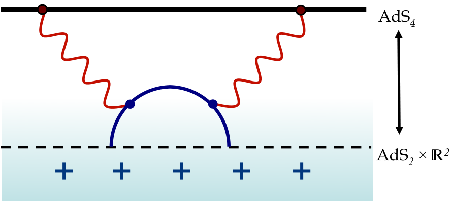
III.4.1 DC conductivity
In many ways this calculation parallels that of Fermi liquid theory, except for the extra bulk dimension and complications from the curved geometry. A main difference comes from the fact that we are performing the computation in a black hole spacetime, meaning that processes such as Figure 13 where the fermion goes through the horizon can contribute. We do not provide any details of the computation here, only pointing out that the final result can be written in terms of boundary theory quantities as
| (131) |
Here is the single-particle spectral function described in the last section, is the Fermi distribution function. All radial integrals have been absorbed into an effective vertex , which takes the schematic form , where is a fermion wavefunction and is a bulk-boundary propagator for the gauge field (which also includes a contribution from the graviton, which mixes with it on this background). This expression can be interpreted in boundary theory terms, as shown in Figure 14; the effect of the radial direction is to provide an exact expression for the renormalized vertex .
In general is a complicated function of all its arguments, but in the low temperature limit and near the Fermi surface it becomes a smooth real function of , independent of and . In this case (131) shows that the conductivity is controlled by the single-particle spectral function near the Fermi surface, and we find the expression
| (132) |
Here is a non-universal number that depends on a radial integral over the bulk fermion wavefunctions (and can be found numerically) but the exponent in is determined by the single-particle decay rate and so by the SLQL. In particular, note that for the Marginal Fermi Liquid case , we find that the contribution to the resistivity from the Fermi surface is linear: , as observed for the cuprates in the strange metal phase and many other non-Fermi liquid materials [10].
Note that in general the electrical transport scattering rate – which emphasizes large momentum transfer – can be different from the single-particle scattering rate. On the other hand in our system the exponent in (132) is determined by the single-particle scattering rate. On the gravity side this arises from the fact that the dissipative portion of the correlation function is determined from Figure 13 essentially by how fast the bulk fermions fall into the black hole, which determines the single-particle decay rate and knows nothing of momentum.2727 27 Note that higher loop diagrams which could potentially spoil this equivalence are suppressed by higher powers of . On the field theory side this is due to the fact that the SLQL sees only the time direction and depends very weakly on momentum.
III.4.2 Optical conductivity
In the computation above the formula (132) for the DC conductivity is rather insensitive to whether or not the Fermi surface has long-lived quasiparticles or not , i.e. the value of . The optical conductivity can also be computed along similar lines; this turns out to depend critically on the value of . Again, we present here only results.
For there are two regimes. In the first we hold fixed in the low temperature limit and find then that we can approximate by a Drude form,
| (133) |
with an overall constant. This is in fact the standard answer for a weakly coupled theory with well-defined quasiparticles, whose lifetime is given by . This should not be surprising; in some sense the effect of holography (in this regime) is to provide the nontrivial lifetime by coupling these quasiparticles to a quantum critical bath. In the other regime (but still ) we find
| (134) |
with a real constant. The term gives us a term proportional to with weight consistent with (133).
On the other hand, for , when we have no long-lived quasiparticles, we find a scale-invariant form,
| (135) |
where is a scaling function that is constant as . For large it falls off as , giving us an optical conductivity with a real constant. This behavior is consistent with a system with no scales and no quasiparticles.
Finally, for the marginal case , we find behavior similar to (135) but with logarithmic violations, i.e.
| (136) |
where again goes to a constant at small . For in this case we find
| (137) |
III.5 SLQL as a fractionalized phase of Fermi liquids
In this subsection we further explore the physics of the oscillatory region discussed in Sec. II.5.3. Such a region exists when
| (138) |
and it is shown in the shaded regions in Fig. 10. In the oscillatory region, the IR scaling dimension of a fermionic operator is complex and the spectral function is nonzero at . At a nonzero , the correlation function (102) is periodic in and has an infinite number of poles in the lower half -plane. It can also be readily checked that all the poles have comparable real and imaginary parts and thus cannot be considered as corresponding to quasiparticles. From the bulk point of view, this region can be interpreted as corresponding to the projection of a bulk Fermi surface (which is one dimension higher) to the boundary. Small excitations at the bulk Fermi surface have a large decay rate since they can fall into the black hole without experiencing any potential barrier.
We will now show that in the parameter range of (138), at any finite the system in fact goes over to a Fermi liquid of “heavy” fermions at low energies. We will keep the boundary spacetime dimension general.
From (109), the local charge density of fermions is given by
| (139) |
where is the volume of a unit sphere in -dimension and is the number of possible spin degeneracies. in (139) is finite and scales as in the large limit2828 28 In contrast the charge density carried by the black hole, given in (47) scales as . which naively implies that the fermionic backreaction can be ignored at leading order. However, the contribution to the boundary charge density from is obtained from integrating it over the radial direction of the black hole, and since in the near horizon region (49) the proper radial distance is infinite and the local proper volume of the transverse is constant, the total boundary density coming from integrating (139) over the radial direction is in fact infinite [95].

The backreaction of the fermionic gas is thus important no matter how large is. The backreacted geometry can be found by using (139) and its corresponding stress tensor as the source for bulk Maxwell and Einstein equations. We refer readers to [95] for details of the calculation and only state the results here. One finds that after taking into account of the backreaction the near-horizon geometry is modified from (107) to a Lifshitz geometry
| (140) |
with
| (141) |
where we have only kept leading order terms in expansion. It is important to emphasize that even in the large limit, the exponential prefector before the second term of (140) cannot be set to unity as it becomes important when is sufficiently large (i.e. ). Also note that as (107), (140) should be used in the region ; the geometry matches to the rest of the rest of black hole (UV region) near .
In the backreacted geometry (140), shown schematically in Figure 15, the local proper volume of the transverse goes to zero as , resulting in a finite boundary fermionic density of order , given by
| (142) |
Plugging the explicit value (141) of into (142) we find that (142) becomes identical to the total charge density (47), i.e. all the charge density of the system is now carried by the fermioinic gas. The black hole has disappeared! It is now replaced by a naked singularity2929 29 Note that at this “singularity” all scalar curvature invariants are actually finite, but nevertheless an observer freely falling into the singularity will feel divergent tidal forces [105]. of zero horizon size and zero charge. The system now also has zero entropy density. Note that such a singularity appears to be of the “good” type allowed by string theory [103, 104]. As we will see below, things could still fall into a singularity, which means in the boundary it should be interpreted as some of “bath” which can dissipate things away. While it has zero entropy and charge at order , likely such a “bath” still carries some charge and entropy at subleading order.
Recall that in obtaining (109) and (139) we used the approximation of a local chemical potential (i.e. Thomas-Fermi approximation), which is valid when are taken to be parametrically large. Thus (141) and (142) are also only valid in this regime.
The Lifshitz geometry (140) is well approximated by (107) until . From the boundary theory perspective, this implies that at an energy scale of order , physics will start deviating from that described by the SLQL. In other words, at sufficiently low energies, the SLQL will order into a new phase which is described by the Lifshitz geometry. What is this new phase? It turns out to be a Fermi liquid of “heavy” fermions [44]! Below we outline the basic arguments, following the treatment of [44], in which more details can be found. Similar calculations appear in [107, 108].
The basic idea is again to examine the retarded Green function for the fermionic operator in which we now expect to find new physics at sufficiently low energies. For this purpose one needs to solve the Dirac equation for the bulk fermions in the backreacted geometry (140), which for and parametrically large can be reduced to a Schrödinger problem describing a particle of zero energy moving in a potential
| (143) |
For the AdS geometry, the first term is simply .
The final results can be readily understood from the qualitative features of the WKB potential (143), as shown in Fig. 16 for . First consider , the potential starts being an almost negative constant for , but eventually rises above zero and approaches as . The Bohr-Sommerfeld quantization condition then leads a series of normalizable bound states at discrete values of . Each such normalizable mode then gives rise a boundary Fermi surface. Alternatively, from the bulk point of view, we now have a bounded potential governing movement in the radial direction. This quantizes the radial modes, and the continuous bulk Fermi surface indicated in Fig. 8 becomes discretized. When projected to the boundary this now become a series of Fermi surfaces as indicated in Fig. 17. Now notice that in (143), for any nonzero no matter how small, the -dependent terms will eventually dominate for sufficiently large and drive the potential to as . This implies bulk particles will eventually fall into the singularity of the Lifshitz geometry and the corresponding boundary fermionic excitations should develop a nonzero width. For exponentially small , there is still a potential barrier and the tunneling rate is exponentially small. In this range there are long-lived quasiparticles. More explicitly, one finds that near each the retarded function for in the range
| (144) |
can be written as
| (145) |
with
| (146) |
Note that since , these are very heavy fermions3030 30 The exponentially small Fermi velocity implies that the effective mass is exponentially large, i.e. . and the decay rate is exponentially small in .
For small but not exponentially small , the first term in (143) is not important for any value of and the potential barrier disappears. One thus recovers previous results of SLQL. In particular, the decay rate becomes and there are no long-lived quasiparticles.
This procedure of solving the Dirac equation in the backreacted geometry (140) is self-consistent and extracts the leading non-perturbative behavior in . There are also perturbative loop corrections in the bulk, which give perturbative corrections in to the self-energy. We expect the qualitative features of the above discussion (e.g the family of densely spaced Fermi surfaces etc) to be robust against these corrections, as they have to do with the global structure of the backreacted geometry (140). Near the Fermi surface perturbative corrections to the self-energy will give rise to a term with some complex coefficient, which will dominate over the imaginary part of in (145) for in the range (144). Thus we expect that the quasiparticle decay rate should be proportional to as in a Landau Fermi liquid.3131 31 Nevertheless, one should keep in mind that the much smaller non-perturbative correction does signal some nontrivial underlying physics beyond that of a Landau Fermi liquid.
We thus see that at low energies the oscillatory region splits into a large number of closely spaced Fermi surfaces whose excitations are Landau quasiparticles. In this regime the Luttinger theorem should hold, which can be checked explicitly (see [44] for details).
Different Fermi surfaces in the family of densely spaced Fermi surfaces can be interpreted as corresponding to different bound states generated by the fermionic operator , as each of them corresponds to a different radial mode in the bulk. Recall that in our set-up, is a composite operator of fundamental fields. The number of degrees of freedom for the fundamental fields is . Thus the Fermi liquid state can be considered a “confined” state, in which the low energy degrees of freedom are Fermi surfaces from a discrete set of composite fermionic bound states. In contrast, the SLQL is a “deconfined” state in which the composite bound states deconfine and fractionalize into more fundamental degrees of freedom. Presumably these more fundamental degrees of freedom account for the entropy density of the SLQL. In the bulk, the emergence of the fractionalized SLQL phase is reflected in the emergence of a charged black hole description. In the Fermi liquid state, the system is characterized by “heavy” fermions. But such coherent quasiparticles disappea in the SLQL. Instead one finds some kind of quantum soup which is characterized by scaling behavior in the time direction for any bosonic or fermionic operators. In the current context the presence of a large number of Fermi surfaces has to do with a spectrum of densely spaced bound states. The fractionalized picture should be independent of this feature. We note also that this interpretation of the SLQL as a fractionalized phase resonates with the lattice model construction of [77], although the details are different.
Note that the WKB potential (143) only includes the near horizon region of the backreacted charged black hole geometry, and does not include the Fermi surfaces discussed in Sec.III.2. In Fig. 18 we show a cartoon of the WKB potential for for the full spacetime, i.e. including the asymptotic AdSd+1 region. The isolated Fermi surfaces discussed earlier in Sec. III.2 and III.3 appear as bound states in a potential well outside the near-horizon region. Such isolated Fermi surfaces exist both in the Fermi liquid phase and in the SLQL, i.e. the corresponding fermionic excitations remain confined in the deconfined SLQL phase. At exponentially small energies, the excitations again become Landau quasiparticles, but with an effective mass.


To summarize, imagine a system with only a single fermionic operator satisfying the condition (138), and no other instabilities. Then at very low energies, the system is described by a Fermi liquid with densely spaced Fermi surfaces, each of size . The quasiparticle excitations have a very large effective mass (proportional to ). There could also be some additional isolated Fermi surfaces with an effective mass. At small but not exponentially small frequencies, there is a wide energy range over which the system is controlled by the SLQL, with scaling behavior in the time direction and various non-Fermi liquid behavior. In the SLQL phase the clue that the system will eventually settles into a Fermi liquid state is the existence of a region , where the scaling dimensions for fermions become complex.
III.6 Generalizations
Before concluding this section, we mention various generalizations which we do not have space to cover.
In the presence of a magnetic field, one can show that fermionic excitations fall into Landau levels [106, 109, 110] and that the free energy displays de-Haas van Alphen oscillations in the inverse magnetic field [111, 112]. The latter calculation also requires a one-loop calculation in the bulk. In [112] it was shown that while the oscillations exist with the expected period, for the amplitude of the oscillations does not take the textbook Lifshitz-Kosevich form. The fermion response in various holographic superconducting phases has been studied in [113, 114, 115, 116, 117, 118, 119]. The superconducting condensate opens a gap in the fermion spectrum around the chemical potential if a certain bulk coupling between the spinor and scalar is included [114]. In particular, in the condensed phase, one finds stable quasiparticles, even when . The properties of Fermi surfaces and associated excitations with more general fermionic couplings or boundary conditions have also been studied in [120, 121, 122, 123] and in more general geometries in [124, 125]. Fermi surfaces in -dimensions were studied in [126, 127, 128]. References [129, 130] considered the pairing instability of holographic non-Fermi liquids.
By considering spinor fields whose mass and charge grows with (i.e. ) and a gauge coupling of order , the Lifshitz geometry (140) has been generalized to have a in [131] (see also [132, 133, 134]). Various aspects of the boundary system dual to such an “electron star” were studied in [135, 136, 137, 107, 108]. In particular, it was found [107, 108] that the fermionic spectral function exhibits multiple Fermi surfaces with exponentially suppressed (in frequency) decay rates very similar to the behavior discussed earlier around (144)–(146) (see also [138] for a hard-wall model for constructing holographic Fermi liquid).
IV Scalar instabilities and quantum phase transitions
The previous section discussed fermions in some detail, describing both non-Fermi liquid physics and the ultimate Fermi-liquid-like ground state of the system. In this section we turn to bosons. Recall from Section II.5 that while fermionic response functions can have gapless modes that describe propagating degrees of freedom (i.e. are in the lower half complex - plane), generically for bosons we instead find instabilities, i.e. poles in the upper half complex plane. This indicates that the scalar operator is trying to condense, and if the operator is charged under any symmetries then they will be broken in the condensed phase.
In this section we examine these bosonic instabilities of the finite charge density system. In particular, when there is an instability we describe how to tune external parameters to make this instability vanish; if this can be done at zero temperature, then this defines a quantum critical point that separates two phases. We will study in detail the critical behavior near such a quantum critical point. We will mainly follow the discussion of [45, 46, 47] (related results have also been obtained in [139, 140, 142], see also [143]). For concreteness we will also specialize to .
We first remind the reader of our setup; consider a CFT3 with a scalar operator . We discussed above in Section II.4 how to use holography to compute the retarded Green’s function of . Before moving on, we will first slightly generalize that discussion to also include double trace deformations in the dual CFT3
| (147) |
It is straightforward to include the presence of such a deformation in our holographic computation. Details are provided in Appendix C; the main result can be found in (274), from which we see that (76) becomes
| (148) |
where
| (149) |
Note that in general the coefficient of the double-trace operator provides a “knob” that can be turned to tune the system through a quantum phase transition.
To follow the standard terminology for discussing phase transitions below we will start calling (148) the susceptibility and use the following notation:
| (150) |
where we distinguish the three only by their arguments. From (148) we find the momentum-dependent and uniform static susceptibilities are given by
| (151) |
and the full dynamical susceptibility takes the form
| (152) |
Below we first recall the instabilities discussed in Sec. II.5 for the system at a finite chemical potential and the corresponding quantum critical points. We will then discuss quantum critical behavior near these quantum critical points.
IV.1 Finite density instabilities
Recall that in II.5 we discussed two possible channels for scalar instabilities, which manifest themselves as presence of poles of (152) in the upper half complex--plane:
- 1.
The SLQL scaling dimension becomes complex for some , for which there are an infinite number of poles in the upper half -plane. Writing (57) as
(153) becomes imaginary for sufficiently small whenever . For a given , this always occurs for a sufficiently large . For a neutral operator , can be negative for lying in the window
(154) where the lower limit comes from the stability of vacuum theory (i.e. BF bound of AdS4) and the upper limit comes from the condition after using the relation (50).
- 2.
can become zero for some special values of momentum . At it is clear from (148) that since , has a singularity at . Furthermore since changes sign near , as discussed in Sec. II.5.1, a pole moves from the upper half -plane (for ) to the lower half -plane (for through . In Fig. 19 we show some examples of a neutral scalar field for which has a zero at some momentum.
In the parameter range (say for ) where either (or both) instability appears, the system is unstable to the condensation of operator (or in bulk language the condensation of ). For a charged scalar the condensed phase is the well-studied holographic superconductor [93, 94]; for reviews see [51, 52]. As was first pointed out in [87], the first instability essentially drives the original construction of the holographic superconductor. Holographic superconductors due to the second type of instability were first discussed in [46].
For a neutral scalar, the first type of instability was first pointed out in [88], and as discussed in [45] the condensed phase can be used as a model for antiferromagnetism when the scalar operator is embedded as part of a triplet transforming under a global symmetry corresponding to spin. For a single real scalar field with a symmetry, the condensed phase can be considered as a model for an Ising-nematic phase. Instabilities of the first type also appear in various other holographic constructions [139, 140]. The potential interaction between these two types of order is discussed in [141].
Both types of instabilities can be cured by going to sufficiently high temperature; there exists a critical temperature , beyond which these instabilities no longer exist and at which the system undergoes a continuous superconducting (for a charged scalar) or antiferromagnetic (for a neutral scalar) phase transition. As have been discussed extensively in the literature [89, 45, 90] such finite temperature phase transitions are of mean field type due to that the boundary conditions at a finite-temperature black hole horizon is analytic.
Alternatively one can continuously dial external parameters of the system at zero temperature to get rid of the instabilities.3232 32 One might be surprised that in the case of a broken continuous symmetry in the ordered phase can persist at any finite temperature, as one generally expects fluctuations of the Goldstone mode to destroy the order. As there is only one Goldstone mode (as compared to other fields) this is a effect and so is dual to a quantum effect in the bulk; it is shown in [144] that at one-loop order in the bulk the symmetry is indeed restored over exponentially long length scales. The critical values of the parameters at which the instabilities disappear then correspond to quantum critical points (QCP) where quantum phase transitions into a superconducting or antiferromagnetic phase occur. We now quickly summarize the nature of each of these quantum critical points.
IV.2 Quantum critical points
IV.2.1 Bifurcating quantum critical point
For the first type of instability a quantum critical point occurs when we violate the Breitenlohner-Freedman bound of the AdS2 region at [45, 139], i.e. from (153), at
| (155) |
For example for a neutral scalar field (with ) this happens at
| (156) |
Note that while in AdS/CFT models the mass square for the vacuum theory is typically not an externally tunable parameter, the effective AdS2 mass square can often be tuned. For example, if we place a holographic superconductor in a magnetic field at zero temperature the AdS2 mass can be changed by tuning the magnetic field [45]. In the set-up of [139], a somewhat different order parameter is dual to a bulk field that has a mass that depends on the external magnetic field. See also [45] for a phenomenological model. Here we will not worry about the detailed mechanism to realize the critical point and will just treat as a dialable parameter (or just imagine dialing the mass square for the vacuum theory). Our main purpose is to identify and understand the critical behavior around the critical point which is independent of the specific mechanism to realize it.
As will be discussed in subsequent sections, as we approach from the uncondensed side (), the static susceptibility remains finite, but develops a cusp at and if we naively continue it to the susceptibility becomes complex. Below we will refer to this critical point as a bifurcating QCP.
IV.2.2 Hybridized quantum critical point
For the second type of instability, one can readily check numerically that is a monotonically increasing function of for negative . See fig. 19. Thus the instability goes away if , which corresponds to satisfying3333 33 There is also an instability for , but one can check that it corresponds to a UV instability of the vacuum. Here we are interested in the IR instability due to finite density effect. See [47] for more discussion.
| (157) |
At the critical point
| (158) |
and as a result the uniform susceptibility in (151) diverges. Such a quantum critical point was first discussed in [46] and elaborated further in [47]. As will be seen below, the presence of the strongly coupled IR sector described by AdS2 gives rise to a variety of new phenomena which cannot be captured by the standard Landau-Ginsburg-Wilson paradigm. For reasons to be clear below, we will refer to such a critical point as a hybridized QCP.
IV.2.3 A marginal quantum critical point
We can also tune and together to have a doubly tuned critical point at , where the susceptibility both diverges and bifurcates. The value of can be obtained from the limit of the expression for given in (157), leading to
| (159) |
where and are constants defined in Eq. (262). For the specific example (156) of tuning the AdS4 mass of a neutral scalar to reach , the values of can be found numerically which give .
As we will see below, the susceptibility around such a critical point coincide with that of the bosonic fluctuations underlying the “Marginal Fermi Liquid” postulated in [12] for describing the strange metal region of the high cuprates.3434 34 It has also been pointed out by David Vegh [145] that the retarded function for a scalar operator with in AdS2 gives bosonic fluctuations of the “Marginal Fermi Liquid”.
We note that while understanding the end point of the instability, i.e. the stable phase in which is condensed, requires full nonlinear analysis of bulk equations, to diagnose the instability, to identify the onset of instability (i.e. the quantum or finite temperature critical points), and to find the critical behavior near the critical points (from the uncondensed side), the linear analysis which gives rise to (148) suffices.
We now proceed to describe the critical behavior near the various critical points identified above. We will use a neutral scalar field for illustration. We should also mention that in all critical points identified above, the uncondensed side is described by an extremal charged black hole. Given the interpretation in Sec. II.6 of an extremal charged black hole as an intermediate state rather than a genuine ground state, the critical behavior discussed below from the uncondensed side should again be interpreted as due to intermediate-energy effects; we return to this point in the conclusion.
IV.3 Quantum Critical behavior: Bifurcating quantum critical point
IV.3.1 Critical behavior
Let us first consider the bifurcating critical point . Here we will outline the results; for details see the recent discussion in [47].
To study the critical behavior from the uncondensed side, we take in (152), i.e. with both and small (in particular, below we will always consider of order or smaller than which is the interesting regime). This limit is a bit subtle as the factor in the SLQL Green function (59) behaves differently depending on the order in which we take the and limits. For example, the Taylor expansion of such a term in small involves terms of the form , but in the small limit, the resulting large logarithms may invalidate the small expansion. We thus proceed carefully. Expanding the explicit form of the AdS2 Green’s function (60) and to leading order in , but keeping the full dependence on , we find that
| (160) |
where
| (161) |
is the Euler number, and are some constants introduced in (262).
This expression is exact for all frequencies that are much smaller than the UV scale; however to understand the physics, we should understand that the non-commutativity of the and limits in equation (160) essentially defines a crossover scale
| (162) |
with some number.
For , one can expand the arguments of the hyperbolic sine to find
| (163) |
with the spectral function given by
| (164) |
However, for , approaching the critical point from the (stable) side, we find
| (165) |
The static susceptibility is obtained from (165) by taking , and interestingly, near the critical point it approaches a finite constant for . It nevertheless develops a branch point singularity at , as ; the susceptibility is trying to bifurcate into the complex plane as we cross . Upon Fourier transformation to coordinate space, this branch point singularity leads to a correlation length that diverges at the critical point. Indeed by comparing (153) with (61), we find that
| (166) |
Thus as , the correlation length diverges as with the same exponent as that in a mean field theory.
When , the SLQL scaling dimension of becomes complex for sufficiently small as is now pure imaginary.3535 35 Note that the choice of branch of the square root does not matter as (160) is an even function of . For a given nonzero and sufficiently small, the corresponding expression for can be obtained from (160) by simply taking , after which we find
| (167) |
For one finds the same critical behavior as (163), but for , we find a geometric series of poles in the upper-half complex frequency-plane at
| (168) |
with
| (169) |
indicating that the disordered state is unstable and the scalar operator condenses in the true vacuum. In particular, we expect (167) to break down for , the largest among (168), and at which scale the physics of condensate sets in. This is indeed consistent with an explicit analysis of classical gravity solutions in [45, 139, 47] where it was found that develops an expectation value of order
| (170) |
The exponent in (170) is the scaling dimension of in the SLQL for , while is its scaling dimension in the vacuum. Furthermore, one in fact finds [45, 139, 47] an infinite tower of excited condensed states in one to one correspondence with the poles in (168)
| (171) |
This tower of condensed states with geometrically spaced expectation values is reminiscent of Efimov states [146].3636 36 In fact the gravity analysis reduces to a quantum mechanical problem which is exactly the same as that for the Efimov states. The state is the ground state with the lowest free energy which scales as (with that of the disordered state being zero)
| (172) |


It is also interesting to compute the response of the system to a static and uniform external source (i.e ) in this tower of “Efimov” states, which turns out to be described by a pair of continuous spiral curves given in Fig. 20 (see [47] for more details). and in the figure denote the source and expectation value for respectively. The set of Efimov states are obtained by setting the source , i.e. they can be read from the intersections of the spirals with the -axis. For comparison we also show the response curve for the standard Landau-Ginsburg story in the right plot of Fig. 20. Approaching the critical point , the spirals exhibit the following features:
- •
The spirals are being squeezed into a straight line, with limiting slope
(173) which agrees with the value found from linear response approaching the critical point from the other side (165).
- •
The susceptibility from the condensed side, which is defined by
(174) however, differs from (173), and is given by
(175) Essentially, even though the spiral is squished into a straight line as we approach the transition, each intersection of the spiral with the axis has a different slope than the limiting slope of the entire spiral. Note that this result is independent of and in particular applies to , the ground state. Since is the value at from the uncondensed side, we thus find a jump in the value of uniform susceptibility in crossing .
The existence of a tower of “Efimov” states with geometrically spaced expectation values may be considered as a consequence of spontaneous breaking of the discrete scaling symmetry of the system. With an imaginary scaling exponent, (167) exhibits a discrete scaling symmetry with (for )
| (176) |
which is, however, broken by the condensate.3737 37 Note that for state, since the physics of the condensate sets in already at , the range of validity for (167) is not wide enough for the discrete scaling symmetry to be manifest. The tower of “Efimov” states may then be considered as the “Goldstone orbit” for this broken discrete symmetry.
At a finite temperature, using the finite generalization of (152) (as discussed at the end of Sec. II.4), equation (160) generalizes to
| (177) |
where is the digamma function. Let us first look at the static regime , for which we find
| (178) |
where some constants of order given by
| (179) |
Similarly to (167), the expression for is obtained by analytically continuing (178) to obtain
| (180) |
Both (178) and (180) are analytic at and for reduce to
| (181) |
When , for equation (178) crosses over to an expression almost identical to (165) with replaced by . For , equation (180) has poles at (for )
| (182) |
Comparing to (182) and (168), we see that . The first of these temperature should be interpreted as the critical temperature
| (183) |
below which the scalar operator condenses and (180) is no longer valid.3838 38 Including frequency dependence, one can check that as is decreased through each , a pole of moves from the lower half -plane to the upper half-plane. Thus we see the interpretation of each of these ; as the temperature is decreased through each of them, one more pole moves through to the upper half-plane. There exist an infinite number of such temperatures with an accumulation point at ; and indeed at strictly zero temperature there is an infinite number of poles in the upper half-plane, as seen earlier in (168). Of course in practice once the first pole moves through to the upper half-plane at , the uncondensed phase is unstable and we should study the system in its condensed phase. One can further study the critical behavior near the finite temperature critical point . Here one finds mean field behavior. Note that equation (180) also has poles with . But such are of order or much larger than for which our approximation is no longer valid, and so we ignore them.
For nonzero , in the quantum critical region , equation (177) becomes
| (184) |
which can now be applied all the way down to zero frequency. Equation (184) reproduces (163) for and (181) for .
In Fig. 21 we summarize the finite temperature phase diagram.

IV.3.2 Physical interpretation: SLQL as a fractionalized phase of Bose condensates
Now let us now try to interpret the above results. First we emphasize that nowhere on the uncondensed side do we see a coherent and gapless quasiparticle pole in the dynamical susceptibility, which usually appears close to a quantum phase transition and indicates the presence of soft order parameter fluctuations. The facts that at the critical point the susceptibility (165) does not diverge and the spectral function (164) is logarithmically suppressed at small frequencies are also manifestations of the lack of soft order parameter fluctuations.
It has been argued in [44, 47] that the quantum phase transition at a bifurcating critical point corresponds to a confinement/deconfinement transition. Across the critical point, the scalar operator develops a complex dimension in the SLQL and conformality is lost. The loss of conformality is realized through a dynamically generated “confinement” scale below which an infinite tower of geometrically separated bound states of operator form and then Bose condense. The physical picture here is similar to the BEC regime in a strongly interacting ultracold Fermi system where fermions form bound molecules and then Bose condense. The bifurcating QCP is thus characterized by the onset of forming bound states rather than by soft order parameter fluctuations; this may help explain why the susceptibility does not diverge at the critical point and the spectral density is suppressed. This should be contrasted with the fermionic case discussed in Sec. III.5, where fermionic bound states each form a Fermi surface. In both cases, SLQL serves as a deconfined high energy state for the more stable lower energy states which arise from SLQL via bound state formation.
To summarize, for a bifurcating QCP, while the phase transition can still be characterized by an order parameter, the order parameter remains gapped at the critical point and the phase transition is not driven by its fluctuations. Instead the phase transition appears to be driven by formation of bound states.
IV.4 Quantum critical behavior: a hybridized QCP
IV.4.1 From uncondensed side
We now examine the critical behavior around a hybridized QCP (158) (again using a neutral scalar) following [46, 47, 142].
The full dynamical behavior from the uncondensed side can be obtained by expanding in (152) around , and , which leads to
| (185) |
with
| (186) |
Recall that the SLQL retarded function . From explicit gravity calculation one finds that the various constants in (185) have the following behavior: , and (for ).
Setting in (185), the static susceptibility can be written as
| (187) |
which has a standard mean field behavior, with the spatial correlation length scaling as
| (188) |
and critical exponents (see Appendix F for a review of definition of critical exponents)
| (189) |
The behavior of the full dynamical susceptibility (185) depends on the competition between the analytic contribution and the non-analytic contribution from SLQL. When , the non-analytic part dominates at low energies and the analytic contribution can be ignored, leading to the interesting and decidedly non-mean-field behavior
| (190) |
where and constant is real and negative for . We will consider below. At the critical point we find that
| (191) |
Away from the critical point, the relative magnitude of the two terms (with ) in the denominator of (190) defines a crossover energy scale
| (192) |
For one finds (187) while for (191). This crossover scale (192) defines the correlation time of the system
| (193) |
Comparing the above expression with (188) we then find that with the dynamical exponent given by
| (194) |
Of course this exponent can equivalently be seen by balancing the term and the term in (190). Also note that when equation (190) has a pole in the upper half plane (since ),
| (195) |
indicating an instability.
When , in (185), the non-analytic part from SLQL becomes less important than the analytic corrections . Since the term proportional to is the only complex term, it should nevertheless be kept. Now (185) describes a long-lived (nearly gapless) relativistic particle with a small width . The dynamical exponent is now .
At a finite temperature , equation (185) generalizes at leading order in to (see discussion at the end of Sec. II.4),
| (196) |
where ( a constant)3939 39 From explicit gravity calculation one finds for . comes from (analytic) finite temperature corrections to and . The finite temperature SLQL retarded function has the form with a universal scaling function (see (69) and (70)). Consider first in (196), which is
| (197) |
It is interesting that the analytic contribution now dominates for . For we find that there is a pole at
| (198) |
for . This should be interpreted as the critical temperature for a thermal phase transition, above which the instability disappears. From the uncondensed side, such a temperature scale coincides with the crossover scale (192). For , we find instead mean field behavior
| (199) |
and the finite temperature crossover scale becomes
| (200) |
which no longer tracks the scale (192) of zero temperature. With nonzero , when , we find scaling, while for there is no scaling.
IV.4.2 Low energy effective action
The discussion in Sec. II.5.2 leading to the low energy effective action (95) for the fermionic case can be applied almost identically to a scalar field. In particular, near a hybridized QCP (158), in (92) can be expanded near and as (say for a neutral scalar)
| (201) |
We thus find that near a hybridized QCP, the low energy effective theory can be written as
| (202) |
where is the same as (97) (except that is now a scalar operator) and
| (203) |
can be considered as the quadratic part of the Landau–Ginsburg action for a scalar order parameter near criticality. The full low energy action (202) describes the hybridization between a Landau-Ginsburg sector and a strongly coupled sector controlled by SLQL. This mixing between two sectors is the key to understanding the critical physics, and is why we call this a hybridized critical point.
The behavior of the dynamical susceptibility at discussed earlier and in particular the crossover to mean field behavior at can be readily seen from the effective action (202). Recall that has SLQL scaling dimension , and from the second term in (202), has dimension . For , the dimension for become smaller than , and as a result the kinetic term (coming from term in (201)) in (203) becomes relevant and more important than the hybridization term (which is marginal by definition) in (202). Alternatively, we can now assign as dimension of using , under which the hybridization term will have dimension which becomes irrelevant for .
The crossover to mean field behavior at at a finite temperature discussed in (197)–(199) can also be readily seen from the effective action (202). Finite temperature can be thought to generate a term , which becomes relevant when the dimension of becomes smaller than zero, i.e. for . Alternatively we can now use term to assign dimension to , under which the hybridization term then becomes irrelevant for as now the dimension for becomes larger than .
Finally, we mention that for there is an alternative description in which the SLQL theory is studied in its alternative quantization, i.e. a different IR operator is used that has dimension . We do not go into details of this description here except to point out that in this description the critical point can be understood as tuning the relevant deformation in the SLQL to . This is thus consistent with the standard Landau-Ginsburg-Wilson paradigm of a critical point as a quantum field theory with a single relevant direction; however the interaction of this relevant direction with the sector described above by the field is nontrivial, resulting in the physics described above. We refer the reader to [46, 47] for more discussion of this.
IV.4.3 Free energy: condensed side
Finally let us look at the the scaling of the expectation value and the free energy from the condensed side. This can be done by analyzing the condensed solution on the gravity side [46]. Alternatively, one could use the low energy effective action (202) [142, 47] which provides a significant simplification. We will use the latter approach. We first generalize (202) by including the next nonlinear term for in (203), i.e.
| (204) |
with some positive constant.
Now consider that develops some nonzero expectation value. From the relative scaling dimensions between and , we can then write as
| (205) |
and the free energy density corresponding to (202) can then be written as
| (206) |
where the first term comes from the term with some constant. Equation (206) can also be derived from a detailed bulk analysis which also gives that for . Now notice that for small, the first term dominates over the term if , while the Landau-Ginsburg term dominates for . In other words, since the first term is marginal by assignment, term becomes relevant when .4040 40 Some readers might worry that higher powers like may also become relevant at some point (for example for ). But note that once the last two terms in (206) dominate we should reassign the dimension of and the standard Landau-Ginsburg story applies.
For we can ignore the last term in (206) and for find that
| (207) |
and as a result
| (208) |
Including the source , which has dimension , the free energy should then be given by a scaling function
| (209) |
where in the second equality we have expressed the free energy in terms of correlation length using (188). From (209) we can also deduce that at the critical point we should have
| (210) |
From (207), (210) and (209) we can collect the values of various scaling exponents (see Appendix F for a review of exponents)
| (211) |
IV.4.4 Summary
We summarize the somewhat intricate critical behavior near a hybridized QCP for various values of in the following table
| Quantity | ||||
|---|---|---|---|---|
| scaling | yes | yes | no | no |
| HYB | HYB | HYB | MFT | |
| HYB | HYB | MFT | MFT | |
| HYB | MFT | MFT | MFT | |
| MFT | MFT | MFT | MFT |
In the above “MFT” denotes mean-field behavior and “HYB” (which is for hybridized) refers to the following non-mean-field exponents for zero-T crossover scale , the dynamical exponent and critical temperature ,
| (214) |
and
| (215) |
For all values of the static susceptibility from the uncondensed side is always given by the mean field behavior (187).
IV.5 Doubly fine-tuning to a marginal critical point
We have just described two different kinds of fixed point; the bifurcating transition involves tuning , and the hybridized transition involves tuning . We can obtain a new kind of critical point by tuning and at the same time, at some critical value given by
| (217) |
where we have used the limit of the expression for given in (157) and are defined in (260)–(262). We will fix and vary .
The dynamical susceptibility can be obtained from the result at the bifurcating critical point (163) and (274)
| (218) |
Now using the definitions of in (161), applying the Wronskian relation (265), and expanding near , we find:
| (219) |
This contains a good deal of interesting physics. First let us keep and study the very low-frequency behavior: expanding in powers of the inverse logarithm, we find
| (220) |
Thus the static susceptibility diverges as , just as for the hybridized critical point discussed above. Away from the critical point the leading contribution to the spectral density appears at order ,
| (221) |
This is the same as the corresponding result close to a bifurcating critical point with zero double-trace deformation.
Next, we note that (219) contains a pole in the upper half plane at
| (222) |
Note however that if , the pole is at an exponentially high energy scale, this low-frequency formula breaks down far before the pole, and the pole is not physical. This is the stable phase. However, if , then close to the critical point the pole is very close to the origin and this formula is valid. The instability pole is now physical, and we see that a new low-energy scale has been exponentially generated. This is reminiscent of the effect of a marginal coupling growing strong in the infrared, as in QCD or the BCS instability. Indeed as discussed in (79) and (80), we expect in the IR a double trace deformation to SLQL will be generated. At , the double trace deformation
| (223) |
has dimension and is thus marginal. It can be checked explicitly that the value of the effective marginal double-trace parameter changes sign at (although one must be somewhat careful; for details see [47]). Thus what we have found above is that if then the coupling is marginally irrelevant and has no effect in the IR, whereas if it is marginally relevant and drives the theory to a new fixed point (i.e. the scalar will condense).
Similarly, one can compute the corresponding finite temperature correlator using (184); a precisely analogous calculation gives
| (224) |
From here we can see that for the static susceptibility diverges at the critical temperature
| (225) |
above which the system is stable. The temperature is set by the same dynamically generated scale.
Now we consider the fluctuation spectrum at criticality. Returning to , we now keep and sit precisely at the critical point . From (219) we now find
| (226) |
The appearance of a pure logarithm in the numerator of this propagator at criticality is interesting. Relatedly, at criticality the spectral density
| (227) |
is a pure step function 4141 41 The logarithm jumps by as we cross through , resulting in the step function; note that this was necessary in order to maintain the relation , true for any bosonic spectral density.. This should be contrasted with the situation away from criticality, (221), in which there is a logarithmic suppression at low frequencies; as expected, by sitting at criticality we find significantly more low frequency modes.
Similarly, setting in the finite temperature expression (224) we find
| (228) |
Taking the imaginary part we find
| (229) |
which is simply a smoothed-out version of the step function that we find at zero temperature. See Fig. 22 for the finite temperature phase diagram for a marginal critical point.
This form of the finite-temperature fluctuation spectrum is potentially of great physical interest. Note that (229) implies that
| (230) |
which is precisely of the form for spin and charge fluctuations in the phenomenological “Marginal Fermi liquid” [12] description of High- cuprates in the strange metal region (as discussed around equation (18) in Sec. I.3). Thus this marginal critical point can be viewed as a concrete realization of the bosonic fluctuation spectrum needed to support a Marginal Fermi liquid.

.
IV.6 Summary
In this section we have discussed several types of quantum critical points related to SLQL which to different degrees lie outside the Landau-Ginsburg-Wilson paradigm:
- •
A hybridized QCP describes an order parameter with a Landau-Ginsburg effective action hybridized with an operator in SLQL. Depending on the scaling dimension of in the SLQL, the phase transition could exhibit a rich spectrum of critical behavior, including locally quantum critical behavior with nontrivial scaling. At the level of effective theory, this critical point lies mildly outside the standard Landau paradigm, as the phase transition is still driven by soft fluctuations of the order parameter and all the critical behavior is fully captured by (202). As discussed in Sec. II.5, on the gravity side the Landau-Ginsburg sector is associated with the appearance of certain scalar hair in the black hole geometry, which lies outside the AdS2 region.
- •
A bifurcating QCP arises from instabilities of the SLQL itself to a confined state and is not driven by soft order parameter fluctuations. On the condensed side, a scalar operator develops a complex scaling dimension in the SLQL, generating a tower of bound states, which then Bose-Einstein condense (the possible bound-states form a geometric series of exponentially generated scales).4242 42 SLQL may be considered as a “deconfined” state in which the composite bound states deconfine and fractionalize into more fundamental degrees of freedom. In particular, one finds a finite critical susceptibility with a branch point singularity, and the response of condensed states is described by an infinite spiral. As discussed in [47], at a field theoretical level, underlying these features is the annihilation (and moving to the complex plane of a coupling constant) of two conformal fixed points, which is very different from the standard Landau-Ginsburg-Wilson paradigm of phase transitions, which can be characterized as a single critical CFT with some relevant directions. On the gravity side, for charged operators the instabilities of the SLQL can be understood as the pair production of charged particles which then subsequently backreact on the geometry. For a neutral scalar operator, the instability is related to the violation of the BF bound in the AdS2 region.
- •
A marginal QCP can be obtained by sitting at the critical point of a bifurcating QCP and then dialing the external parameter which drives a hybridized QCP. Here given the critical theory describing a bifurcating QCP (which comes from the merger of two fixed points), the phase transition can be described as the appearance of a marginally relevant operator. Interestingly, the fluctuation spectrum that emerges is identical to the bosonic fluctuation spectrum that (when coupled to a Fermi surface) is postulated to underly the “Marginal Fermi Liquid” description of the optimally doped cuprates [12], making this critical point of potential importance.

Finally let us elaborate on an important point, which we have glossed over in our discussion so far. As discussed in Sec. II.6, SLQL, which describes the disordered phase in our examples above, should be interpreted an intermediate-energy phase, rather than a genuine ground state. That is, we expect SLQL to order into some other phases at lower energies, which may not be visible at the large limit we are working with. An example discussed in Sec. III.5 is that at some exponentially small scale in , SLQL orders into a Fermi liquid phase.4343 43 See [143] for a recent discussion of nucleation of a neutral order parameter in a Fermi liquid-like phase. Thus the quantum critical behavior found in this paper should be more correctly interpreted as describing the intermediate-region indicated in Fig. 23.
V Discussion and conclusions
In these lectures, we used gauge/gravity duality to study a class of finite density systems, which are described on the gravity side by a charged black hole. We showed that the duality predicts a universal intermediate-energy phase, called a semi-local quantum liquid (SLQL). Such an unstable phase is characterized by a finite spatial correlation length, but an infinite correlation time and associated nontrivial scaling behavior in the time direction, as well as a nonzero entropy density. We discussed two sets of phenomena related to the SLQL:
- 1.
Gapless fermionic or bosonic degrees of freedom (described by mean field) hybridized with degrees of freedom in SLQL. In either case, the system can be described by the following low energy effective theory
(231) In the fermionic case, denotes excitations around a Fermi surface with given by that for a free fermion (plus possibly higher order self-interactions). In the bosonic case, denotes the order parameter around a quantum critical point with its Landau-Ginsburg effective theory. In both cases, is some (fermionic or bosonic) operator whose dynamics is controlled by the strongly coupled SLQL. The IR behavior of the theory (i.e. whether one finds a Fermi surface with or without quasiparticles, or a quantum phase transition which obeys locally quantum critical or mean-field behavior) depends crucially on the scaling dimension of in the SLQL. With a suitable choice of the SLQL scaling dimension, IR phenomena which strongly resemble those of high- cuprates in the strange metal phase (including a linear resistivity) and that for near a quantum critical point were found.
On the gravity side the gapless degrees of freedom are associated with the appearance of certain scalar or fermionic hair in the black hole geometry, and lie outside the AdS2 region which describes the SLQL.
- 2.
Instabilities of the SLQL itself. We discussed examples in which SLQL orders at lower energies to a Fermi liquid, superconductor, or antiferromagnetic-type state. In all cases certain operators develop a complex scaling dimension in the SLQL generating a tower of bound states. In the fermion case, each of these bound states forms a Fermi surface. In the scalar case, they form a tower of Bose-Einstein condensed states. In particular, near the bifurcating critical point where the scalar instability sets in one finds a finite susceptibility and the response is described by an infinite spiral. In all of these examples the lower energy states have no zero-temperature entropy density and SLQL may be considered as a “deconfined” state for them in which the composite bound states deconfine and fractionalize into more fundamental degrees of freedom. This may help explain the nonzero entropy density for the SLQL. As discussed in Sec. II.6, we expect this picture to be generic; while the precise nature of the lower energy state depends on the specific dynamics of the individual system, the SLQL emerges universally at intermediate energies through fractionalization.
Instabilities of SLQL in turn provide novel mechanisms for the emergence of Fermi liquids, superconductors and AFM-type of states at low energies.
On the gravity side, for charged operators the instabilities of the SLQL manifest themselves as pair production of charged particles which then subsequently backreact on the geometry. For a neutral scalar operator, the instability is related to the violation of the BF bound in the AdS2 region.
It is natural to ask whether some phase similar to the SLQL could underlie some known strongly correlated condensed matter systems, and in particular, whether the observed non-Fermi liquid behavior and novel superconductivities in various systems could be attributed to a similar intermediate-energy phase.
When one encounters scaling behavior in an observable, an important immediate question is whether the behavior is due to intermediate-energy or vacuum effects. Here we provide an explicit example in which Marginal Fermi Liquid behavior – such as that proposed for high- cuprates in the strange metal phase (including linear resistivity) – can arise from intermediate energy effects. Local quantum critical behavior similar to that for near a quantum critical point also appears here as due to intermediate energy effects.
In many heavy electron systems, while quantum fluctuations from the quantum critical point corresponding to the onset of magnetism provide a natural starting point for understanding the observed non-Fermi liquid behavior and sometimes novel superconductivity, however, such exotic behavior does not always arise in the proximity of a quantum critical point (see e.g. [10]). There thus appears plenty of room for them to arise from an intermediate-energy phase.
More generally, we expect that candidates for the SLQL to occur include systems which exhibit frustrated or competing interaction terms in their Hamiltonian. Such systems can have a large number of near-degenerate states near the vacuum, similarly to the holographic systems considered here. Also systems which involve strong competition between tendencies towards itinerancy and localization could exhibit the semi-local behavior found here. As mentioned earlier, there are also some tantalizing parallels between properties of the SLQL phase and models from dynamical mean field theory (DMFT) [33], such as scaling in the time direction with spatial directions as spectators, and a finite entropy. The fact that DMFT techniques have been very successful in treating many materials in some intermediate energy region provides some comfort in thinking that an underlying universal intermediate-energy phase like the SLQL could be at work.
Acknowledgements
We thank T. Faulkner, J. McGreevy, D. Vegh, and Q. Si for collaborations. We also want to thank participants of TASI 2010, KITPC workshop for “AdS/CM and other approaches,” and IIP school on “Holographic View of Condensed Matter Physics” for many questions and discussions, which helped shape these lectures. We also want to thank K. Balasubramanian, H. Ebrahim, T. Grover, G. Kotliar, J. Maldacena, J. Polchinski, S. Sachdev for useful discussions. Work supported in part by funds provided by the U.S. Department of Energy (D.O.E.) under cooperative research agreement DE-FG0205ER41360.
Appendix A Operator dimensions and retarded functions in AdS2
Here we give a derivation of the scaling dimension (56)-(57) and retarded Green’s function (59) for a charged scalar in AdS. The background metric and gauge field is given by (49) which we copy here for convenience
| (232) |
We consider the following quadratic scalar action
| (233) |
Expanding in terms of Fourier modes in spatial directions,
| (234) |
equation (233) reduces to an action for in AdS2
| (235) |
with a mass square
| (236) |
The indices only run over . Further going to frequency space one finds that equation of motion from (235) can be written as (for notational simplicity we will just denote as below)
| (237) |
with
| (238) |
where
| (239) |
Approaching the AdS2 boundary , equation (237) has general solution
| (240) |
Compare (240) to (26); it implies that the conformal dimension of the operator to has dimension , as claimed in (56) and (57).
Introducing , equation (237) can be written as
| (241) |
which is precisely the Whittaker’s equation and the two linearly independent solutions can be written as
| (242) |
where is the Whittaker function. Of these, the function multiplying ,
| (243) |
is ingoing at the horizon. Keeping only the ingoing part, the asymptotic behavior of at is given by
| (244) |
From (30) the retarded function is simply the ratio of two coefficients in the above equation, leading to
| (245) |
which is (59).
Appendix B Derivation of the master formula
Here we present the derivation of the master formula (76), following [40]. The equation of motion (in momentum space) for with action (233) in the charged black hole geometry (33) can be written as
| (246) |
We will consider with and given by (45). Recall from (26) that near the AdSd+1 boundary has the standard asymptotic behavior and that the correlator we seek to compute can be written as4444 44 We will consider the standard quantization in our discussion below. The generalization to the alternative quantization is immediate.
| (247) |
provided that is an in-falling wave at the horizon. Note that since as , the boundary theory energy corresponds to , i.e. should be interpreted as the measured from the effective chemical potential (which we take to be positive for definiteness).
We are interested in the behavior of in the low frequency limit (). However, we cannot directly perform a perturbative expansion in in (246) since the -dependent term becomes singular and dominates at the horizon where , no matter how small is. This is not just a technicality; physically this reflects the abundance of critical modes coming from the IR fixed point and is of tremendous importance.
To deal with it, it is useful to isolate the near-horizon AdS region (49) (which will be referred to as the IR region) from the rest of the black hole spacetime (which will be referred to as the UV region). In the IR AdS2 region the dependence will be treated non-perturbatively. The crossover between the two regions happens near the boundary of AdS2 with , where remains big so that we are still in the near-horizon region, but the -dependent term in (246) becomes small. In the UV region we can treat the small limit using a standard perturbative expansion with the lowest order equation given by setting in (246).
So we start with a solution in the AdS region and evolve it outwards, matching it to a solution in the UV region to determine the coefficients and . The scalar wave equation on the AdS region (49) is given by (237). As we are computing a retarded correlator we are looking for an in-falling solution at the black hole horizon (i.e. the term proportional to in (242) even though the explicit form is not important for the current discussion). We now take this infalling solution and evolve it to the boundary of the AdS2 region, where it can be written as
| (248) |
In (248) we have normalized the solution so that the first term has coefficient and then by definition the coefficient of the second term is precisely the retarded Green function in the AdS2 region we computed earlier in (245).
We now need to continue evolution all the way to the asymptotically AdSd+1 region to extract the coefficients and . We thus need to match the IR solution (248) to a solution in the UV region. Now that we are out of the dangerous IR region, to leading order we can set in (246) in the UV region,
| (249) |
The above equation has two independent solutions which can be specified by their behavior near as
| (250) |
with the corresponding asymptotic behavior as as
| (251) |
and thus defined are (dimensionless) functions of which can be computed numerically.
In the overlapping region both (248) and (250) apply, which determines the full UV solution to be
| (252) |
Equation (252) can be generalized to higher orders in (for details see [40])
| (253) |
where
| (254) |
are the two linearly independent perturbative solutions to the full UV region equation. Near , have the expansion of the form (251) with various coefficients replaced by which have an analytic -expansion such as
| (255) |
Note that since both the boundary conditions specifying (250) and the equation (246) are real, are real. From (253) and the expansion of near we thus find the boundary theory Green’s function to be
| (256) |
We conclude this discussion with some remarks:
- 1.
At , the leading order equation (249) in the outer region is in fact the full equation of motion; there is no IR region. of (250) now provide a set of basis for the full equation of motion. Note that by construction is normalizable at the horizon. When vanishes, from (251) becomes normalizable also at the boundary and thus is now a genuine normalizable mode in the black hole geometry.
- 2.
- 3.
The functions are obtained by solving equation (246) perturbatively in in the UV region. Their -dependence comes from two sources, from dependence on via the boundary condition (250) and from dependence in the equation (246) itself. Since the geometry is smooth throughout the UV region we expect the dependence on both and to be analytic. In fact we can think of and as functions of ; i.e. there exists a function , analytic in all its arguments, such that . This is clear from the boundary condition (250) (and its generalization for higher orders in ) and from the fact that there is no other dependence on from the equation of motion itself.
- 4.
As , the two solutions in (250) become degenerate, i.e.
(258) At , the basis of functions in (250) should be replaced by
(259) where the asymptotic behavior for them at is
(260) are now dimensionless real numbers which can again be found numerically. More explicitly, in the limit of the basis of functions (250) can be expanded as
(261) which leads to
(262) - 5.
Coefficients are not independent. For example evaluating the Wronskian of (246) (for )4545 45 The Wronskian of equation (246) is given by (263) which is independent of . for and demanding that it be equal at infinity and at the horizon, we find the elegant relation:
(264) A similar analysis on results in
(265) - 6.
When is pure imaginary (i.e. when (99) is satisfied), and the basis of solutions (250) now has the form
(266) These boundary conditions are now complex, and thus so are the . As the actually obey a real wave equation, the full analytic structure is determined by the boundary conditions in the infrared; thus we find that now . This also implies that are complex and
(267) - 7.
The derivation leading to (256) can be immediately generalized to a finite temperature . In the IR region one replaces the equation (237) by the corresponding equation for the AdS2 black hole (52). As a result, in (248) is now replaced its finite-temperature generalization (69). The outer region discussion is exactly the same as before except that one should use finite temperature counterparts of and in (249). For , the outer region equation depends on analytically and the asymptotic behavior in equations (250) and (251) is unchanged. Thus for , one simply replaces in (256) by , but keeping in mind that now also have analytic temperature dependence.
Appendix C Double trace deformations
Consider a large gauge theory in Euclidean signature deformed by a double-trace operator
| (268) |
where is a scalar operator whose Euclidean correlation function (in the absence of deformation) is given by . With this deformation the two point function for now becomes:
| (269) | |||||
| (270) |
which leads to
| (271) |
The disconnected diagrams cancel between the numerator and denominator, leaving us with only connected diagrams. To leading order in the large limit, the -th term in the above equation becomes
| (272) |
In momentum space we thus find a simple geometric sum
| (273) |
Analytically continuing (273) to the Lorentzian signature and using the standard relation between the Euclidean and retarded functions we conclude that
| (274) |
where and are retarded functions for before and after the double trace deformation.
For a CFT, the Euclidean correlator in momentum space for an operator can be written as
| (275) |
where where is the scaling dimension of and is some constant factor. Plugging the above equation into (273) we find that for ,
| (276) |
This is expected, since for , the double trace deformation (268) is irrelevant and the theory flows back to the original fixed point in the IR. When , for which (268) is relevant, we find that in the IR
| (277) |
The first term in the above equation is a constant (which gives rise to a contact term in coordinate space) and can be ignored. The second term corresponds to an operator of dimension . We thus conclude that under the double trace deformation the system flows to a new CFT in the IR in which has dimension . Note that two-point functions of other operators (which are orthogonal to ) are unaffected.
In the bullet below that of equation (30) in Sec.(II.1) we mentioned that for , there are two ways to quantize a scalar field in AdS. In the standard quantization (Dirichlet boundary condition) the corresponding boundary operator has dimension , while in the alternative quantization (Neumann boundary condition), the corresponding boundary operator has dimension . From our discussion above, upon turing on a double trace operator in the alternative quantization, in the large limit the system should flow in the IR to a new fixed point in which has dimension with the dimensions of all other operators unchanged. Clearly this new fixed point should be identified with that corresponding to the standard quantization.
Appendix D Fourier transforms
Consider an integral of the form
| (278) |
where with and some constants. We will assume that the analytic structure of is such that the only singularities in the complex -plane are at the beginning of the branch cuts in , that is at . If that is so, then we can take the two branch cuts to go upwards and downwards in the complex -plane and then (for positive ) by deforming the contour upwards we can rewrite the above integrand as
| (279) |
Now in the limit of large we expect the integral to be dominated by the lower limit of the integrand . We can expand the sub-exponential part of the integrand in powers of and perform the integrals directly; thus it is clear that the leading behavior will be of the form
| (280) |
where the power appearing in depends on the exact form of the integrand. The key point here is the the location of the branch cut sets a scale which determines the correlation length in the integral.
Appendix E Density of states of semi-local quantum liquids
In this Appendix we consider the density of states of a semi-local quantum liquid. The discussion is motivated by a recent argument of [92], which appears to indicate that scaling symmetry only in the time direction cannot persist to arbitrarily low energies. The argument is very simple and goes as follows. On dimensional grounds, the scaling symmetry in the time direction implies that the density of states of such a theory should have the form
| (281) |
where and are constants. The term proportional to gives rise to an entropy density, while the term proportional to appears to be needed to have any nontrivial dynamics (as otherwise the Hamiltonian will be proportional to the identity operator in this sector). With , however, the integral of the term is divergent at low energies, suggesting an infinite number of states at arbitrarily low energies. This peculiar result suggests that the scaling symmetry must always break down at sufficiently low energies, say below some new dynamically generated scale . Note that the argument is independent of the existence of a ground state entropy density, i.e. it should apply even if .4646 46 For example, it will rule out the kind of local quantum critical point discussed in the literature (e.g. [29]) as a genuine low energy description of of certain quantum phase transitions in heavy fermion materials.
We note, however, there are some subtleties with the argument. In order to have a finite density of states we should introduce an IR cutoff, i.e. we should put the system in a finite box with volume , and (281) applies to the system in a finite box. Even without a new dynamically generated scale , in a finite box, we expect that the system should develop a finite gap with
| (282) |
in the thermodynamic limit . Thus, more precisely, the argument for a new dynamically generated scale should be made in the thermodynamic limit, i.e. should remain finite for . Let us now assume that such an does not exist, and see whether one can find an immediate contradiction from (281) in the thermodynamic limit.
In general it is hard to deal with the total density of states of an interacting system. In the thermodynamic limit, we can instead consider entropy whose exponential can be considered as giving the total density of states. Thus we first translate equation (281) into a statement regarding the entropy. For , taking the logarithm of (281) we find
| (283) |
The term is singular in the limit, but note that this singular term is not proportional to the volume, and thus appears to be negligible in the thermodynamic limit. This by itself does not imply that (281) is fine with . But it does indicate that drawing a conclusion requires going beyond the thermodynamic limit, in which case one will need to worry about the precise boundary conditions, shape of the box, and etc. In particular, given that the finite volume cutoff breaks the scaling symmetry, it is not clear whether (281) is really valid. To further highlight possible subtleties associated with going outside the thermodynamic limit, note that there is an alternative way to obtain the entropy from (281),
| (284) |
In the thermodynamic limit this definition is equivalent to simply taking the logarithm of the density of states. But applying (284) to (281) we find that
| (285) |
where we have put an IR cutoff in the integration of (284). The -dependence in (285) differ from that in (283). In the limit the second term in is singular, but the divergence is much smaller than volume factor in the usual thermodynamic limit.
The above discussion does motivate a stronger argument based on the thermodynamic limit. Instead of (281) one may argue that the scaling symmetry in the time direction implies that the entropy of the system should have the form
| (286) |
where for convenience we have used the canonical ensemble and are -independent constants. Argument similar to that below (281) again seems to say that nontrivial dynamics requires , which then implies that the system should have a dynamically generated cutoff in the thermodynamic limit. We note, however, the coefficient of the term may not be required to be nonzero to have nontrivial dynamics, as the systems which exhibit such a scaling symmetry have a UV completion. The leading contribution could come from an irrelevant operator. We will discuss a potential example below.
For a boundary theory at finite density described by a charged black hole in the bulk, the entropy has the form
| (287) |
The term comes from the black hole geometry. The term proportional to comes from a one-loop calculation in the bulk. It is a well defined question to ask whether has a singular piece in the limit. Here we will not attempt a full one-loop calculation. To get an indication of the behavior of , we compute instead the single-particle density of states4747 47 It should be kept in mind this bulk single-particle density of states does not correspond to any single-particle density of states in the boundary. for a scalar field in AdS. Using one obtains an “off-shell” partition function using the standard formulas
| (288) |
where is the single-particle partition function in the bulk. We would like to see whether there is a singular term in which can be traced to a similar term in 4848 48 The standard one loop partition function at a finite which can be used to directly extract is computed from path integral in the Euclidean black hole geometry with given . There exists argument (see e.g. [147]) that the “off-shell” partition function we are considering is equivalent to that computed from Euclidean path integral. Clearly it would be desirable to compute the Euclidean partition function directly. .
Before going into technical details, let us summarize the results:
- A.
For a scalar in AdS, introducing a finite volume in the field-theory spatial directions does not result in a finite density of states in the bulk4949 49 As emphasized earlier the relation of this bulk single-particle density of states with the density of states in the boundary theory is rather indirect. In particular, one should not view the cutoff introduced below as a new emergent dynamical scale. As discussed in [147] the divergence of in the limit in fact is identical to UV divergences in the Euclidean partition functions. , due to the presence of the horizon. To proceed, we will thus introduce an additional cutoff where is a radial coordinate cutoff of the spacetime above the horizon.
- B.
Within this regularization scheme, for a scalar operator of real scaling dimension in SLQL, the dangerous piece is not present. Instead the leading cutoff-independent contribution in the density of states comes from an irrelevant operator (a double trace deformation) and is integrable at small . One finds that and thus the corresponding contribution to goes to zero in the limit.
- C.
For an operator with complex scaling dimension in SLQL, one does find a non-vanishing (cutoff-independent) piece in the single-particle density of states. Upon integration, this leads to a singular single-particle partition function and thus a singular . We would conclude that in this case, a new dynamical scale should emerge in the thermodynamic limit. This is in nice correspondence with the discussion of sec. II.5.3, where we show that precisely in this case the system is unstable to the condensate of the scalar operator and thus a new dynamical scale must emerge. We expect similar results should also apply to a fermionic operator with a complex dimension, which will again be in nice correspondence with the fermionic instability discussed in Sec. III.5.
From the above, it then appears that the argument based on (281) or (286) alone is not enough to rule out the presence of a scaling symmetry in the time direction persisting to arbitrarily low energies; it seems that dynamics still plays a role in determining whether this is possible. Clearly further study of this is desirable.
E.1 Single-particle density of states in the bulk
Here we calculate the density of states of a neutral scalar field in AdS, whose equation of motion is given by (237)–(239) with . We will consider solutions which are normalizable at the boundary5050 50 For definiteness we will restrict to the standard quantization., i.e. in (240). At the horizon , the correponding wave function is given by a plane wave
| (289) |
with a phase shift. Note that the normalizable condition and a discrete does not impose a quantization condition on ; the system has a continuous spectrum (we are dealing with a scattering problem) even with a finite volume cutoff. While we expect that the system should develop a discrete spectrum in a finite volume, the spacings of low-lying spectrum could be much smaller than , with is the system size, in the large and large limit, and thus not immediately visible at our level of approximation. Thus in order to obtain a finite density of states, we will impose an IR cutoff by hand at near the horizon5151 51 should be -dependent, but we will not specify the dependence.. has units of time and is the inverse of the energy cutoff scale discussed above. This now requires that satisfies
| (290) |
Taking differential on both sides of the last equation we find that
| (291) |
We thus conclude that the density of states is given by
| (292) |
where is the cutoff-independent part given by
| (293) |
Now note that the scaling symmetry of AdS2 implies that the phase shift is in fact independent as the only dependence of a wave function on should be through . Thus (293) is identically zero and we are left with a piece which depends on the cutoff.
E.1.1 Double trace deformation
The above discussion is, however, not the full story as the AdS2 region appears in the IR part of the full black hole geometry, which provides the UV completion. As discussed in Sec. II.4 (see discussion around equation (80)), the leading irrelevant deformation of SLQL is provided by the double trace operator, which we now consider. With a double trace deformation, the normalizable solution is now given by setting
| (294) |
in (240). Note that the double trace parameter has dimension . Up to an overall scaling the normalizable condition can also be written as
| (295) |
The full normalizable solution in AdS2 then has the form
| (296) |
We thus find the phase shift is given by
| (297) |
For small we thus find that
| (298) |
which when plugged into (293) leads to
| (299) |
where denotes higher order corrections in . The above density of states is integrable at .5252 52 Recall that for , . We thus find that that the cutoff-independent part of the density of states is controlled by leading irrelevant perturbation.
E.2 Imaginary
Let us now consider an imaginary . For notational simplicity we will now drop the momentum subscript. Embedding the AdS2 into the full extremal BH geometry) amounts to requiring the normalizable wave function to have the asymptotic behavior near the AdS2 boundary
| (300) |
for some choice of (which depends on ), whose precise value will not concern us. The full normalizable solution in AdS2 is then almost identical to (296) with now imaginary
| (301) | |||||
| (302) |
with
| (303) |
Note that in contrast to the earlier case, is now dimensionless, which indicates that now has to be proportional to on dimensional ground. The phase shift is now given by
| (304) |
We thus conclude that
| (305) |
which has an un-integrable singularity at . Note that including the momentum integrations in (293) will not cure this non-integrability as is almost independent for .
Appendix F Review of critical exponents
In the vicinity of a critical point we observe scaling behavior of various observable quantities, which is characterized by a set of critical exponents. We list some of the most commonly used exponents in the following. We will denote the external tuning parameter with which we tune the system to the critical point . Near the critical point the spatial correlation length diverges as
| (306) |
The energy gap for elementary excitations scales as
| (307) |
where is called the dynamic critical exponent and determines the characteristic time scale of the approach to equilibrium via . On the condensed side the order parameter also exhibits scaling near the critical point; the corresponding exponent is:
| (308) |
and exactly at the critical point it will depend on the source as
| (309) |
where the coupling to the external source is . The correlation function can also be used to probe the physical properties of the critical point. The next critical exponent we introduce is for at zero momentum:
| (310) |
The decay of at the critical point in the free theory would be , the deviation from this is characterized by :
| (311) |
To study the scaling of thermodynamic functions we introduce as:
| (312) |
where is the free energy density.
References
- [1] J. M. Maldacena, “The large N limit of superconformal field theories and supergravity,” Adv. Theor. Math. Phys. 2, 231 (1998) [Int. J. Theor. Phys. 38, 1113 (1999)] [arXiv:hep-th/9711200].
- [2] S. S. Gubser, I. R. Klebanov and A. M. Polyakov, “Gauge theory correlators from non-critical string theory,” Phys. Lett. B 428, 105 (1998) [arXiv:hep-th/9802109];
- [3] E. Witten,“Anti-de Sitter space and holography,” Adv. Theor. Math. Phys. 2, 253 (1998) [arXiv:hep-th/9802150]
- [4] S. S. Gubser, A. Karch, “From gauge-string duality to strong interactions: A Pedestrian’s Guide,” Ann. Rev. Nucl. Part. Sci. 59, 145-168 (2009). [arXiv:0901.0935 [hep-th]].
- [5] J. Casalderrey-Solana, H. Liu, D. Mateos, K. Rajagopal and U. A. Wiedemann, “Gauge/String Duality, Hot QCD and Heavy Ion Collisions,” arXiv:1101.0618 [hep-th].
- [6] P. Coleman, “Introduction to Many-body Physics,” http://www.physics.rutgers.edu/coleman.
- [7] G. Benfatto and G. Gallavotti, “Renormalization-Group Approach to the Theory of the Fermi Surface,” Phys. Rev. B 42 (1990) 9967.
- [8] J. Polchinski, “Effective Field Theory and the Fermi Surface,” arXiv:hep-th/9210046.
- [9] R. Shankar, “Renormalization group approach to interacting fermions,” Rev. Mod. Phys. 66, 129 (1994).
- [10] G. R. Stewart, “Non-Fermi-liquid behavior in d- and f-electron metals,” Rev. Mod. Phys. 73, 797 (2001).
- [11] E. Abrahams and C. M. Varma, “What angle-resolved photoemission experiments tell about the microscopic theory for high-temperature superconductors,” PNAS 97, 5714 (2000).
- [12] C. M. Varma, P. B. Littlewood, S. Schmitt-Rink, E. Abrahams, and A. E. Ruckenstein, “Phenomenology of the normal state of Cu-O high-temperature superconductors,” Phys. Rev. Lett. 63, 1996 – 1999 (1989).
- [13] T. Holstein, R. E. Norton and P. Pincus, “de Haas-van Alphen Effect and the Specific Heat of an Electron Gas,” Phys. Rev. B 8, 2649 (1973); P. A. Lee and N. Nagaosa, “Gauge theory of the normal state of high-Tc superconductors,” Phys. Rev. B 46, 5621 (1992); M. Y. Reizer, Phys. Rev. B 40, 11571 (1989); J. Polchinski, “Low-energy dynamics of the spinon-gauge system,” Nucl. Phys. B 422, 617 (1994) arXiv:cond-mat/9303037; C. Nayak and F. Wilczek, “Non-Fermi liquid fixed point in (2+1)-dimensions,” Nucl. Phys. B 417, 359 (1994) arXiv:cond-mat/9312086, “Renormalization group approach to low temperature properties of a non-Fermi liquid metal,” Nucl. Phys. B 430, 534 (1994) arXiv:cond-mat/9408016; B. I. Halperin, P. A. Lee and N. Read, “Theory of the half filled Landau level,” Phys. Rev. B 47, 7312 (1993); Y. B. Kim, A. Furusaki, X.-G. Wen, and P. A. Lee, “Gauge-invariant response functions of fermions coupled to a gauge field,” Phys. Rev. B 50, 17917–17932 (1994); B. L. Altshuler, L. B. Ioffe and A. J. Millis, “On the low energy properties of fermions with singular interactions,” Phys. Rev. B 50 14048 (1994). [arXiv:cond-mat/9406024].
- [14] S. S. Lee, “Low energy effective theory of Fermi surface coupled with U(1) gauge field in 2+1 dimensions,” Phys. Rev. B 80, 165102 (2009) [arXiv:0905.4532 [cond-mat.str-el]].
- [15] M. A. Metlitski and S. Sachdev, “Quantum phase transitions of metals in two spatial dimensions: I. Ising-nematic order,” Phys. Rev. B 82, 075127 (2010) [arXiv:1001.1153 [cond-mat.str-el]].
- [16] D. F. Mross, J. McGreevy, H. Liu and T. Senthil, “A controlled expansion for certain non-Fermi liquid metals,” Phys. Rev. B 82, 045121 (2010) [arXiv:1003.0894 [cond-mat.str-el]].
- [17] J. A. Hertz,“Quantum critical phenomena,” Phys. Rev. B 14, 1165–1184 (1976).
- [18] S. Sachdev, Quantum Phase Transitions, Cambridge University Press, Cambridge (1999).
- [19] M. A. Continentino, Quantum scaling in many-body systems, World Scientific, Singapore, (2001).
- [20] S. L. Sondhi, S. M. Girvin, J.P. Carini, D. Shahar, “Continuous quantum phase transitions,”’ Rev. Mod. Phys. 69, 315-333 (1997) [ arXiv:cond-mat/9609279]
- [21] M. Vojta, “Quantum phase transitions,” Rep. Prog. Phys. 66, 2069 (2003), [arXiv:cond-mat/0309604].
- [22] Focus issue: Quantum phase transitions, Nature Phys. 4, 167–204 (2008).
- [23] P. Gegenwart, Q. Si, and F. Steglich, “Quantum criticality in heavy-fermion metals,” Nat. Phys. 4, 186–197 (2008).
- [24] H. v. Löhneysen, A. Rosch, M. Vojta, and P. Wölfle, “Fermi-liquid instabilities at magnetic quantum phase transitions,” Rev. Mod. Phys. 79, 1015–1075 (2007).
- [25] X.-G. Wen, “Vacuum degeneracy of chiral spin states in compactified space,”Phys. Rev. B 40, 7387 (1989).
- [26] X.-G. Wen and Q. Niu, “Ground-state degeneracy of the fractional quantum Hall states in the presence of a random potential and on high-genus Riemann surfaces,” Phys. Rev. B41, 9377 (1990).
- [27] P. Coleman, “Heavy Fermions: electrons at the edge of magnetism”, arXiv:cond-mat/0612006.
- [28] Q, Si and F. Steglich, “Heavy Fermions and Quantum Phase Transitions,” Science 329, 1161 (2010).
- [29] Q. Si, S. Rabello, K. Ingersent, and J. L. Smith, “Locally critical quantum phase transitions in strongly correlated metals,” Nature 413, 804–808 (2001).
- [30] T. Senthil, A. Vishwanath, L. Balents, S. Sachdev, and M. P. A. Fisher, “Deconfined quantum critical points,” Science 303, 1490–1494 (2004).
- [31] A. Schröder, G. Aeppli, R. Coldea, M. Adams, O. Stockert, H. v. Lohneysen, E. Bucher, R. Ramazashvili, and P. Coleman, “Onset of antiferromagnetism in heavy-fermion metals,” Nature 407, 351 (2000).
- [32] P. Coleman, “Theories of non-Fermi liquid behavior in heavy fermions,” Physica B 259-261, 353 (1999).
- [33] A. Georges, G. Kotliar, W. Krauth, M. J. Rozenberg, “Dynamical mean-field theory of strongly correlated fermion systems and the limit of infinite dimensions,” Rev. Mod. Phys. 68, 13-125 (1996); G. Kotliar, S. Y. Savrasov, K. Haule, V. S. Oudovenko, O. Parcollet, and C. A. Marianetti, “Electronic structure calculations with dynamical mean-field theory,” Rev. Mod. Phys. 78, 865 (2006).
- [34] J. Bagger and N. Lambert, “Comments On Multiple M2-branes,” JHEP 0802, 105 (2008) [arXiv:0712.3738 [hep-th]]; “Gauge Symmetry and Supersymmetry of Multiple M2-Branes,” Phys. Rev. D 77, 065008 (2008) [arXiv:0711.0955 [hep-th]]; “Modeling multiple M2’s,” Phys. Rev. D 75, 045020 (2007) [arXiv:hep-th/0611108].
- [35] A. Gustavsson, “Algebraic structures on parallel M2-branes,” Nucl. Phys. B 811, 66 (2009) [arXiv:0709.1260 [hep-th]].
- [36] O. Aharony, O. Bergman, D. L. Jafferis and J. Maldacena, “N=6 superconformal Chern-Simons-matter theories, M2-branes and their gravity duals,” JHEP 0810, 091 (2008) [arXiv:0806.1218 [hep-th]].
- [37] S.-S. Lee, “A Non-Fermi Liquid from a Charged Black Hole; A Critical Fermi Ball,” Phys. Rev. D 79, 086006 (2009) [arXiv:0809.3402 [hep-th]].
- [38] H. Liu, J. McGreevy, and D. Vegh, “Non-Fermi liquids from holography,” arXiv:0903.2477 [hep-th].
- [39] M. Cubrovic, J. Zaanen, and K. Schalm, “String Theory, Quantum Phase Transitions and the Emergent Fermi-Liquid,” Science 325, 439–444 (2009) [arXiv:0904.1993 [hep-th]].
- [40] T. Faulkner, H. Liu, J. McGreevy, and D. Vegh, “Emergent quantum criticality, Fermi surfaces, and AdS2,” arXiv:0907.2694 [hep-th].
- [41] T. Faulkner, N. Iqbal, H. Liu, J. McGreevy and D. Vegh, “Strange metal transport realized by gauge/gravity duality,” Science 329, 1043-1047 (2010); arXiv:1003.1728 [hep-th].
- [42] T. Faulkner, N. Iqbal, H. Liu, J. McGreevy and D. Vegh, “Holographic non-Fermi liquid fixed points,” arXiv:1101.0597 [hep-th].
- [43] T. Faulkner and J. Polchinski, “Semi-Holographic Fermi Liquids,” arXiv:1001.5049 [hep-th].
- [44] N. Iqbal, H. Liu and M. Mezei, “Semi-local quantum liquids,” arXiv:1105.4621 [hep-th].
- [45] N. Iqbal, H. Liu, M. Mezei and Q. Si, “Quantum phase transitions in holographic models of magnetism and superconductors,” arXiv:1003.0010 [hep-th].
- [46] T. Faulkner, G. T. Horowitz and M. M. Roberts, “Holographic quantum criticality from multi-trace deformations,” arXiv:1008.1581 [hep-th].
- [47] N. Iqbal, H. Liu and M. Mezei, “Quantum phase transitions in semi-local quantum liquids,” arXiv:1108.0425 [hep-th].
- [48] C. P. Herzog, P. Kovtun, S. Sachdev and D. T. Son, “Quantum critical transport, duality, and M-theory,” Phys. Rev.Ê D 75, 085020 (2007) [arXiv:hep-th/0701036].
- [49] S. Sachdev, M. Mueller, “Quantum criticality and black holes,” 0810.2005 [cond-mat.str-el]
- [50] S. A. Hartnoll, “Lectures on holographic methods for condensed matter physics,” Class. Quant. Grav. 26, 224002 (2009) [arXiv:0903.3246 [hep-th]].
- [51] C. P. Herzog, “Lectures on Holographic Superfluidity and Superconductivity,” J. Phys. A 42, 343001 (2009) [arXiv:0904.1975 [hep-th]].
- [52] G. T. Horowitz, “Introduction to Holographic Superconductors,” arXiv:1002.1722 [hep-th].
- [53] S. J. Rey, “String Theory on Thin Semiconductors,” Progress of Theoretical Physics Supplement No. 177 (2009) pp. 128-142; arXiv:0911.5295 [hep-th].
- [54] S. Sachdev, “Condensed matter and AdS/CFT,” arXiv:1002.2947 [hep-th].
- [55] S. A. Hartnoll, “Horizons, holography and condensed matter,” arXiv:1106.4324 [hep-th].
- [56] S. Sachdev, “What can gauge-gravity duality teach us about condensed matter physics?,” arXiv:1108.1197 [cond-mat.str-el].
- [57] J. P. Gauntlett, J. Sonner and D. Waldram, “The spectral function of the supersymmetry current (I),” arXiv:1106.4694 [hep-th].
- [58] R. Belliard, S. S. Gubser and A. Yarom, “Absence of a Fermi surface in classical minimal four-dimensional gauged supergravity,” arXiv:1106.6030 [hep-th].
- [59] I. Bah, A. Faraggi, J. I. Jottar and R. G. Leigh, “Fermions and Type IIB Supergravity On Squashed Sasaki-Einstein Manifolds,” JHEP 1101, 100 (2011) [arXiv:1009.1615 [hep-th]].
- [60] I. Bah, A. Faraggi, J. I. Jottar, R. G. Leigh and L. A. Pando Zayas, “Fermions and Supergravity On Squashed Sasaki-Einstein Manifolds,” JHEP 1102, 068 (2011) [arXiv:1008.1423 [hep-th]].
- [61] J. P. Gauntlett, J. Sonner and T. Wiseman, “Holographic superconductivity in M-Theory,” Phys. Rev. Lett. 103, 151601 (2009) [arXiv:0907.3796 [hep-th]].
- [62] J. P. Gauntlett, J. Sonner and T. Wiseman, “Quantum Criticality and Holographic Superconductors in M-theory,” JHEP 1002, 060 (2010) [arXiv:0912.0512 [hep-th]].
- [63] S. S. Gubser, C. P. Herzog, S. S. Pufu and T. Tesileanu, “Superconductors from Superstrings,” Phys. Rev. Lett. 103, 141601 (2009) [arXiv:0907.3510 [hep-th]].
- [64] F. Aprile, D. Roest and J. G. Russo, “Holographic Superconductors from Gauged Supergravity,” arXiv:1104.4473 [hep-th].
- [65] A. Donos and J. P. Gauntlett, “Superfluid black branes in AdS,” arXiv:1104.4478 [hep-th].
- [66] J. Polchinski, “Introduction to Gauge/Gravity Duality,” arXiv:1010.6134 [hep-th].
- [67] J. McGreevy, “Holographic duality with a view toward many-body physics,” Adv. High Energy Phys. 2010, 723105 (2010) [arXiv:0909.0518 [hep-th]].
- [68] L. Susskind and E. Witten, “The Holographic bound in anti-de Sitter space,” arXiv:hep-th/9805114.
- [69] A. W. Peet and J. Polchinski, “UV / IR relations in AdS dynamics,” Phys. Rev. D 59, 065011 (1999) [arXiv:hep-th/9809022].
- [70] D. T. Son, A. O. Starinets, “Minkowski space correlators in AdS / CFT correspondence: Recipe and applications,” JHEP 0209, 042 (2002). [hep-th/0205051].
- [71] See e.g., S. Coleman, “”, in Aspect of Symmetry, Cambridge Univ. Press, (1985).
- [72] L. J. Romans, “Supersymmetric, cold and lukewarm black holes in cosmological Einstein-Maxwell theory,” Nucl. Phys. B 383, 395 (1992) arXiv:hep-th/9203018.
- [73] A. Chamblin, R. Emparan, C. V. Johnson and R. C. Myers, “Charged AdS black holes and catastrophic holography,” Phys. Rev. D 60, 064018 (1999) arXiv:hep-th/9902170.
- [74] S. Sachdev and J. Ye, “Gapless spin-fluid ground state in a random quantum Heisenberg magnet,” Phys. Rev. Lett. 70, 3339 (1993).
- [75] L. Zhu and Q. Si, “Critical local-moment fluctuations in the Bose-Fermi Kondo model,” Phys. Rev. B 66, 024426 (2002); L. Zhu, S. Kirchner, Q. Si, and A. Georges, “Quantum Critical Properties of the Bose-Fermi Kondo Model in a Large-N Limit,” Phys. Rev. Lett. 93, 267201 (2004).
- [76] S. Burdin, D. R. Grempel, and A. Georges, “Heavy-fermion and spin-liquid behavior in a Kondo lattice with magnetic frustration,” Phys. Rev. B 66, 045111 (2002).
- [77] S. Sachdev, “Holographic metals and the fractionalized Fermi liquid,” Phys. Rev. Lett. 105, 151602 (2010) [arXiv:1006.3794 [hep-th]].
- [78] S. J. Yamamoto, Q. Si, “Global Phase Diagram of the Kondo Lattice: From Heavy Fermion Metals to Kondo Insulators,” J. Low Temp. Phys. 161, 233 (2010) [arXiv:1006.4868].
- [79] S. Sachdev, “The landscape of the Hubbard model,” [arXiv:1012.0299 [hep-th]].
- [80] L. Huijse, S. Sachdev, “Fermi surfaces and gauge-gravity duality,” [arXiv:1104.5022 [hep-th]].
- [81] T. Faulkner, H. Liu and M. Rangamani, “Integrating out geometry: Holographic Wilsonian RG and the membrane paradigm,” arXiv:1010.4036 [hep-th].
- [82] I. Heemskerk and J. Polchinski, “Holographic and Wilsonian Renormalization Groups,” arXiv:1010.1264 [hep-th].
- [83] N. Iqbal and H. Liu, ‘Real-time response in AdS/CFT with application to spinors,” Fortsch. Phys. 57, 367 (2009) [arXiv:0903.2596 [hep-th]].
- [84] P. Breitenlohner and D. Z. Freedman, “Stability In Gauged Extended Supergravity,” Annals Phys. 144, 249 (1982).
- [85] S. S. Gubser, “Phase transitions near black hole horizons,” Class. Quant. Grav. 22, 5121 (2005) [arXiv:hep-th/0505189].
- [86] S. S. Gubser and A. Nellore, “Low-temperature behavior of the Abelian Higgs model in anti-de Sitter space,” JHEP 0904, 008 (2009) [arXiv:0810.4554 [hep-th]].
- [87] F. Denef and S. A. Hartnoll, “Landscape of superconducting membranes,” arXiv:0901.1160 [hep-th].
- [88] S. A. Hartnoll, C. P. Herzog and G. T. Horowitz, “Holographic Superconductors,” JHEP 0812, 015 (2008) [arXiv:0810.1563 [hep-th]].
- [89] K. Maeda, M. Natsuume and T. Okamura, “Universality class of holographic superconductors,” Phys. Rev. D 79, 126004 (2009) [arXiv:0904.1914 [hep-th]].
- [90] C. P. Herzog, “An Analytic Holographic Superconductor,” Phys. Rev. D81, 126009 (2010). [arXiv:1003.3278 [hep-th]].
- [91] B. Pioline and J. Troost, “Schwinger pair production in AdS(2),” JHEP 0503, 043 (2005) [arXiv:hep-th/0501169].
- [92] K. Jensen, S. Kachru, A. Karch, J. Polchinski and E. Silverstein, “Towards a holographic marginal Fermi liquid,” arXiv:1105.1772 [hep-th].
- [93] S. S. Gubser, “Breaking an Abelian gauge symmetry near a black hole horizon,” Phys. Rev. D 78, 065034 (2008) [arXiv:0801.2977 [hep-th]];
- [94] S. A. Hartnoll, C. P. Herzog and G. T. Horowitz, “Building a Holographic Superconductor,” Phys. Rev. Lett. 101, 031601 (2008) [arXiv:0803.3295 [hep-th]].
- [95] S. A. Hartnoll, J. Polchinski, E. Silverstein and D. Tong, “Towards strange metallic holography,” arXiv:0912.1061 [hep-th].
- [96] S. Nakamura, H. Ooguri and C. S. Park, “Gravity Dual of Spatially Modulated Phase,” Phys. Rev. D 81, 044018 (2010) [arXiv:0911.0679 [hep-th]]; H. Ooguri and C. S. Park, “Holographic End-Point of Spatially Modulated Phase Transition,” Phys. Rev. D 82, 126001 (2010) [arXiv:1007.3737 [hep-th]].
- [97] S. S. Gubser and F. D. Rocha, “Peculiar properties of a charged dilatonic black hole in AdS5,” Phys. Rev. D 81, 046001 (2010) [arXiv:0911.2898 [hep-th]].
- [98] K. Goldstein, S. Kachru, S. Prakash and S. P. Trivedi, “Holography of Charged Dilaton Black Holes,” JHEP 1008, 078 (2010) [arXiv:0911.3586 [hep-th]].
- [99] K. Goldstein, N. Iizuka, S. Kachru, S. Prakash, S. P. Trivedi and A. Westphal, “Holography of Dyonic Dilaton Black Branes,” JHEP 1010, 027 (2010) [arXiv:1007.2490 [hep-th]].
- [100]
C. Charmousis, B. Gouteraux, B. S. Kim, E. Kiritsis and R. Meyer,
“Effective Holographic Theories for low-temperature condensed matter
systems,”
JHEP 1011, 151 (2010)
[arXiv:1005.4690 [hep-th]];
R. Meyer, B. Gouteraux and B. S. Kim, “Strange Metallic Behaviour and the Thermodynamics of Charged Dilatonic Black Holes,” arXiv:1102.4433 [hep-th];
B. Gouteraux, B. S. Kim and R. Meyer, “Charged Dilatonic Black Holes and their Transport Properties,” arXiv:1102.4440 [hep-th]. - [101] J. McGreevy, “In pursuit of a nameless metal,” A Viewpoint on [77], Physics 3, 83 (2010).
- [102] P. W. Anderson, “In Praise of Unstable Fixed Points: The Way Things Actually Work,” arXiv:cond-mat/0201431.
- [103] S. S. Gubser, “Curvature singularities: The Good, the bad, and the naked,” Adv. Theor. Math. Phys. 4, 679 (2000) [arXiv:hep-th/0002160].
- [104] J. M. Maldacena and C. Nunez, “Supergravity description of field theories on curved manifolds and a no go theorem,” Int. J. Mod. Phys. A 16, 822 (2001) [arXiv:hep-th/0007018].
- [105] S. Kachru, X. Liu, M. Mulligan, “Gravity Duals of Lifshitz-like Fixed Points,” Phys. Rev. D78, 106005 (2008). [arXiv:0808.1725 [hep-th]].
- [106]
T. Albash and C. V. Johnson,
“Holographic Aspects of Fermi Liquids in a Background Magnetic Field,”
arXiv:0907.5406 [hep-th];
T. Albash and C. V. Johnson, “Landau Levels, Magnetic Fields and Holographic Fermi Liquids,” J. Phys. A 43, 345404 (2010) [arXiv:1001.3700 [hep-th]]. - [107] S. A. Hartnoll, D. M. Hofman and D. Vegh, “Stellar spectroscopy: Fermions and holographic Lifshitz criticality,” arXiv:1105.3197 [hep-th].
- [108] M. Cubrovic, Y. Liu, K. Schalm, Y. W. Sun and J. Zaanen, “Spectral probes of the holographic Fermi groundstate: dialing between the electron star and AdS Dirac hair,” arXiv:1106.1798 [hep-th].
- [109] P. Basu, J. He, A. Mukherjee and H. H. Shieh, “Holographic Non-Fermi Liquid in a Background Magnetic Field,” arXiv:0908.1436 [hep-th].
- [110] E. Gubankova, J. Brill, M. Cubrovic, K. Schalm, P. Schijven and J. Zaanen, “Holographic fermions in external magnetic fields,” arXiv:1011.4051 [hep-th].
- [111] F. Denef, S. A. Hartnoll and S. Sachdev, “Black hole determinants and quasinormal modes,” Class. Quant. Grav. 27, 125001 (2010) [arXiv:0908.2657 [hep-th]]; F. Denef, S. A. Hartnoll and S. Sachdev, “Quantum oscillations and black hole ringing,” Phys. Rev. D 80, 126016 (2009) [arXiv:0908.1788 [hep-th]].
- [112] S. A. Hartnoll and D. M. Hofman, “Generalized Lifshitz-Kosevich scaling at quantum criticality from the holographic correspondence,” Phys. Rev. B 81, 155125 (2010) [arXiv:0912.0008 [cond-mat.str-el]].
- [113] J. W. Chen, Y. J. Kao and W. Y. Wen, “Peak-Dip-Hump from Holographic Superconductivity,” arXiv:0911.2821 [hep-th].
- [114] T. Faulkner, G. T. Horowitz, J. McGreevy, M. M. Roberts and D. Vegh, “Photoemission ‘Experiments’ on Holographic Superconductors,” arXiv:0911.3402 [hep-th].
- [115] S. S. Gubser, F. D. Rocha and P. Talavera, “Normalizable Fermion Modes in a Holographic Superconductor,” arXiv:0911.3632 [hep-th].
- [116] S. S. Gubser, F. D. Rocha and A. Yarom, “Fermion correlators in non-abelian holographic superconductors,” arXiv:1002.4416 [hep-th].
- [117] M. Ammon, J. Erdmenger, M. Kaminski and A. O’Bannon, “Fermionic Operator Mixing in Holographic p-wave Superfluids,” JHEP 1005, 053 (2010) [arXiv:1003.1134 [hep-th]].
- [118] F. Benini, C. P. Herzog and A. Yarom, “Holographic Fermi arcs and a d-wave gap,” arXiv:1006.0731 [hep-th].
- [119] D. Vegh, “Fermi arcs from holography,” arXiv:1007.0246 [hep-th].
- [120] M. Edalati, R. G. Leigh and P. W. Phillips, “Dynamically Generated Mott Gap from Holography,” Phys. Rev. Lett. 106, 091602 (2011) [arXiv:1010.3238 [hep-th]].
- [121] M. Edalati, R. G. Leigh, K. W. Lo and P. W. Phillips, “Dynamical Gap and Cuprate-like Physics from Holography,” Phys. Rev. D 83, 046012 (2011) [arXiv:1012.3751 [hep-th]].
- [122] D. Guarrera and J. McGreevy, “Holographic Fermi surfaces and bulk dipole couplings,” arXiv:1102.3908 [hep-th].
- [123] J. N. Laia and D. Tong, arXiv:1108.1381 [hep-th].
- [124] T. Albash, “Non-Unitary Fermionic Quasinormal Modes at Zero Frequency,” arXiv:1002.4431 [hep-th].
- [125] J. P. Wu, “Holographic fermions in charged Gauss-Bonnet black hole,” arXiv:1103.3982 [hep-th].
- [126] J. R. Wang and G. Z. Liu, “Non-Fermi liquid behavior due to U(1) gauge field in two dimensions,” Nucl. Phys. B 832, 441 (2010) [arXiv:0907.1022 [cond-mat.supr-con]].
- [127] V. Balasubramanian, I. Garcia-Etxebarria, F. Larsen and J. Simon, “Helical Luttinger Liquids and Three Dimensional Black Holes,” arXiv:1012.4363 [hep-th].
- [128] M. Rangamani and B. Withers, “Fermionic probes of local quantum criticality in one dimension,” arXiv:1106.3210 [hep-th].
- [129] T. Hartman and S. A. Hartnoll, “Cooper pairing near charged black holes,” JHEP 1006, 005 (2010) [arXiv:1003.1918 [hep-th]].
- [130] E. Gubankova, “Particle-hole instability in the holography,” arXiv:1006.4789 [hep-th].
- [131] S. A. Hartnoll and A. Tavanfar, “Electron stars for holographic metallic criticality,” arXiv:1008.2828 [hep-th].
- [132] J. de Boer, K. Papadodimas and E. Verlinde, “Holographic Neutron Stars,” JHEP 1010, 020 (2010) [arXiv:0907.2695 [hep-th]].
- [133] X. Arsiwalla, J. de Boer, K. Papadodimas and E. Verlinde, “Degenerate Stars and Gravitational Collapse in AdS/CFT,” JHEP 1101, 144 (2011) [arXiv:1010.5784 [hep-th]].
- [134] M. Cubrovic, J. Zaanen and K. Schalm, “Constructing the AdS dual of a Fermi liquid: AdS Black holes with Dirac arXiv:1012.5681 [hep-th].
- [135] S. A. Hartnoll, D. M. Hofman and A. Tavanfar, “Holographically smeared Fermi surface: Quantum oscillations and Luttinger count in electron stars,” arXiv:1011.2502 [hep-th].
- [136] S. A. Hartnoll and P. Petrov, “Electron star birth: A continuous phase transition at nonzero density,” arXiv:1011.6469 [hep-th].
- [137] V. G. M. Puletti, S. Nowling, L. Thorlacius and T. Zingg, “Holographic metals at finite temperature,” JHEP 1101, 117 (2011) [arXiv:1011.6261 [hep-th]].
- [138] S. Sachdev, “A model of a Fermi liquid using gauge-gravity duality,” arXiv:1107.5321 [hep-th].
- [139] K. Jensen, A. Karch, D. T. Son and E. G. Thompson, “Holographic Berezinskii-Kosterlitz-Thouless Transitions,” arXiv:1002.3159 [hep-th].
- [140] K. Jensen, “More Holographic Berezinskii-Kosterlitz-Thouless Transitions,” Phys. Rev. D 82, 046005 (2010) [arXiv:1006.3066 [hep-th]].
- [141] P. Basu, J. He, A. Mukherjee, M. Rozali and H. H. Shieh, JHEP 1010, 092 (2010) [arXiv:1007.3480 [hep-th]].
- [142] K. Jensen, “Semi-Holographic Quantum Criticality,” arXiv:1108.0421 [hep-th].
- [143] M. Edalati, K. W. Lo and P. W. Phillips, “Neutral Order Parameters in Metallic Criticality in d=2+1 from a Hairy Electron Star,” arXiv:1106.3139 [hep-th].
- [144] D. Anninos, S. A. Hartnoll and N. Iqbal, “Holography and the Coleman-Mermin-Wagner theorem,” Phys. Rev. D 82, 066008 (2010) [arXiv:1005.1973 [hep-th]].
- [145] D. Vegh, “Marginal Fermi liquids at holographic quantum critical points,” unpublished.
- [146] V. Efimov, “Energy levels arising from resonant two-body forces in a three-body system,” Phys. Lett. B33, 563 (1970).
- [147] D. V. Fursaev, Nucl. Phys. B 524, 447 (1998) [arXiv:hep-th/9709213].