1.44
![[Uncaptioned image]](1110.3577v1/mono_large.png)
The University of Adelaide
School of Chemistry and Physics
Discipline of Physics
Chiral Effective Field Theory
Beyond the Power-Counting Regime
Jonathan Michael MacGillivray Hall
Supervisors: Prof. Derek B. Leinweber, Dr. Ross D. Young
Special Research Centre for the
Subatomic Structure of Matter
and
Department of Physics,
University of Adelaide,
Australia
June 2011
Abstract
Chiral effective field theory complements numerical simulations of quantum chromodynamics on a spacetime lattice. It provides a model-independent formalism for connecting lattice simulation results at finite volume, and at a variety of quark masses, to the physical region. Knowledge of the power-counting regime of chiral effective field theory, where higher-order terms of the expansion may be regarded as negligible, is as important as knowledge of the expansion. Through the consideration of a variety of renormalization schemes, techniques are established to identify the power-counting regime. Within the power-counting regime, the results of extrapolation are independent of the renormalization scheme.
The nucleon mass is considered as a benchmark for illustrating this approach. Because the power-counting regime is small, the numerical simulation results are also examined to search for the possible presence of an optimal regularization scale, which may be used to describe lattice simulation results outside of the power-counting regime. Such an optimal regularization scale is found for the nucleon mass. The identification of an optimal scale, with its associated systematic uncertainty, measures the degree to which the lattice QCD simulation results extend beyond the power-counting regime, thus quantifying the scheme-dependence of an extrapolation.
The techniques developed for the nucleon mass renormalization are applied to the quenched meson mass, which offers a unique test case for extrapolation schemes. In the absence of a known experimental value, it serves to demonstrate the ability of the extrapolation scheme to make predictions without prior phenomenological bias. The robustness of the procedure for obtaining an optimal regularization scale and performing a reliable chiral extrapolation is confirmed.
The procedure developed is then applied to the magnetic moment and the electric charge radius of the isovector nucleon, to obtain a consistent optimal regularization scale. The consistency of the results for the value of the optimal regularization scale provides strong evidence for the existence of an intrinsic energy scale for the nucleon-pion interaction.
Statement of Originality
This work contains no material which has been accepted for the award of any other degree or diploma in any university or other tertiary institution to Jonathan Hall and, to the best of my knowledge and belief, contains no material previously published or written by another person, except where due reference has been made in the text.
I give consent to this copy of my thesis, when deposited in the University Library, being available for loan and photocopying, subject to the provisions of the Copyright Act 1968.
I also give permission for the digital version of my thesis to be made available on the web, via the University’s digital research repository, the Library catalogue and also through web search engines, unless permission has been granted by the University to restrict access for a period of time.
Acknowledgments
Thank you to Professor Derek Leinweber, for his patient and intelligent supervision and his sense of humour expressed during our enjoyable discussions. Also thank you to Doctor Ross Young for his explanations of theory, his patience, and for our numerous, informative conversations. Ross’ generosity with his time for me has been exemplary, and in many cases, an essential component of our successes.
I also thank Doctor Rod Crewther, who has been very informative in the fields of physics and education, and Doctor James Zanotti, who has helped marvellously with collaboration and support.
Thank you to the staff of the School of Chemistry and Physics for their general assistance, and more specifically to Professor Anthony Thomas and the staff of the Special Research Centre for the Subatomic Structure of Matter.
I give my thanks to my loving family for their support.
It is with hope and faith that we endeavour to extend our learning to reach new insights just beyond our present reach.
Chapter 1 Introduction
“One measure of the depth of a physical theory is the extent to which it poses serious challenges to aspects of our worldview that had previously seemed immutable.” (Greene, B. 1999. The Elegant Universe p.386) [Gre99]
1.1 Prologue
The theoretical physicist challenges previous theory, using original research that enables alternative coherence to emerge, as outlined by Bohm [Boh92] (p.223). The underlying theory behind the strong force of particle interactions, which is the force responsible for the binding of protons and neutrons together in atomic nuclei, had been a persistent mystery throughout the first half of the Twentieth Century. This hitherto unknown force acts in opposition to the electric Coulomb force that repels positively charge protons from each other, but is at least two orders of magnitude stronger at the distance scale of an atomic nucleus. The strong interaction between protons and neutrons, or nucleons, is currently most successfully described by the theory of quantum chromodynamics (QCD). The advent of the quark model, and the theory of the colour force by which the quarks interact, opened a new field of research into the internal structure of matter.
In 1964, Gell-Mann and Zweig independently proposed the existence of a new constituent particle, the quark, in order to classify the bewildering array of subatomic particles called hadrons [GM64]. It was discovered that the hadrons can be arranged into families that correspond to representations of the group , and that three quark types, or flavours, were required to form the fundamental representation of this group. It was not until 1968 that the results of deep inelastic scattering experiments provided the first evidence of the existence of these new elementary particles. As more hadrons were discovered, additional quark flavours were proposed. It is currently accepted that six flavours of quark are required to produce the full range of hadrons observed in particle accelerator experiments. Their names, in ascending order of mass, are: up, down, strange, charm, bottom and top. Of the six flavours, the most recent to be discovered experimentally was the top quark, in 1995 at Fermilab, with a mass of 172 GeV [Pro96].
Each quark has a unit of charge equal to or times the charge of a proton (units of ). An an example, the proton consists of two up quarks and a down quark for a total charge of , whereas a neutron consists of two down quarks and an up quark for a total charge of zero. However, because quarks have a certain spatial distribution inside the nucleon, or indeed any hadron, the internal, high energy dynamics as described by the behaviour of quarks gives rise to properties such as non-zero magnetic moments for the neutron and anisotropic momentum distributions. It is clear that in order to describe the internal behaviour of a hadron, one cannot assume that a quark behaves as a static source. Instead, the dynamics of quarks must be described by a theory, the most successful of which is QCD.
QCD connects the quark model of nuclear physics to quantum gauge field theories by introducing the quarks as the relevant degrees of freedom inside a hadron. The hadrons are formed by confined colour singlets of three quarks called baryons, or quark-antiquark pairs, known as mesons. Quarks are spin- fermions, which also have the properties of colour and approximate flavour symmetry. Since fermions, by definition, must satisfy Fermi-Dirac statistics, the fact that each baryon contains three bound quarks in the same state violates the Pauli Exclusion Principle. Therefore, it was necessary to suppose an the existence of an additional quantum number, known as colour charge, so that each quark may be assigned one of three, orthogonal basis states, labelled red, green and blue. Colour is mediated by the related gauge particles of the strong force; the gluons, and the quarks also form a representation of the colour gauge group , with eight group generators.
Mathematically, QCD is a non-Abelian theory. That is, the gauge connection of the gluons is non-commutative. The fact that isolated, unbound quarks are never found in experiment is one of the striking consequences of a non-Abelian theory. Confinement of the quarks within a hadron is a result of the gluon fields exerting a linear potential that increases with distance between quarks [Wil74]. That is, for a large distance scale, the strong coupling parameter also becomes large. This behaviour contrasts with electromagnetism, where the electric Coulomb force diminishes as two charged particles are separated. However, quarks experience only a small force from the gluon fields as becomes small at short distances [GW73b, Pol73, GW73a, GW74]. This asymptotic freedom is observed when probing the internal structure of hadron at high energies, where the small de Broglie wavelength of the probe is able to resolve the short distances within the composite particle. Near this asymptotically free regime, the methods of perturbative quantum field theory are suitable for constructing amplitudes, cross-sections and scattering matrices. However, it leads to a difficulty in finding an appropriate method for performing a calculation with QCD in the low-energy region. Two of the most successful methods that will be discussed in this thesis are chiral effective field theory (EFT) and lattice QCD.
Using EFT, one is able to encapsulate the dynamics of a quantum system by writing down an ‘effective’ action of low-energy degrees of freedom. By imposing symmetries satisfied by QCD, one can expand out the formula for an observable property into a series of quantum amplitudes that can be arranged in order of the importance of their contribution by a choice of power-counting scheme: usually in increasing powers of mass/energy. These amplitudes can alter, or renormalize the calculation of an observable from its naïve value, and landmark success has been made in confirming these real and measurable effects by experiment. For example, the value of the anomalous magnetic dipole moment of the electron agrees with experiment to better than twelve significant figures. The Casimir effect (1948), which describes the forces arising from the quantum vacuum fluctuations, were successfully predicted by the gauge field theory of quantum electrodynamics (QED). In the low-energy, non-perturbative region of QCD, many phenomena can be explained by the emergent properties of quark confinement and the behaviour of their bound states as hadrons. For example, the proton and neutron also have a large anomalous component of their magnetic moment. This is due to the cloud of interacting fields, which renormalize the core of the observable. This ‘hadron cloud’ is one of the unique properties of a quantum field theory. Of the available low-energy effective theories of QCD, chiral perturbation theory (PT) is the most notable, in its careful incorporation of the fundamental symmetries of QCD. However, the robustness of PT is confined only to a restrictive region called the power-counting regime. Within the power-counting regime, the perturbative expansions that occur in PT are convergent; the terms of the expansion series are ordered such that higher-order terms are sufficiently smaller than lower-order terms. The details of the power-counting regime are discussed in more detail in Chapter 3.
Lattice QCD is a discretized version of QCD, where the dynamics are evaluated on a finite-sized box with only certain allowed values of position (or momentum) separated by a fixed spacing. Thus, lattice QCD is equivalent to QCD in the limit of infinite box size and vanishing lattice spacing. Using lattice QCD, one is able to access the non-perturbative, low-energy regime of QCD and provide reliable predictions of hadronic behaviour. In addition, lattice QCD simulations do not suffer from the common problems of quantum field theory associated with renormalization. The discrete lattice spacing and the finite box size of the lattice act as an ultraviolet and infrared regulator, respectively. Thus, observable quantities evaluated on the lattice are finite and calculable. Nevertheless, it can be computationally expensive to evaluate observables at large box sizes, small lattice spacings and physical quark masses. To be able to obtain a result using quark masses as small as their physical values, an extrapolation is a practical alternative to a brute-force approach. In addition, the corrections to finite-volume effects ought also to be calculated for a realistic comparison with experiments.
1.2 Overview and Aims
The framework of QCD provides a rich selection of possibilities for inquiry. Among these, the low-energy, chiral dynamics of hadrons provides us with a uniquely successful understanding of many of their imporant properties.
This thesis explores the properties of the aforementioned power-counting regime by considering how low-energy constants, which occur in a calculation using the methods of PT, are renormalized, or altered, at different energy scales. This knowledge of the power-counting regime, in turn, yields insight into the repercussions of chiral symmetry breaking in QCD.
The results of lattice QCD simulations provide an important application for the investigation into PT and the power-counting regime. Lattice QCD results are typically produced at a variety of quark masses larger than the physical quark mass. As such, a chiral extrapolation to the physical point is required before the result can be compared to experiment. In addition, experimental results are not constrained by the boundaries of a small box only a few fermi in length. It is important to be able to quantify how the finite-volume nature of lattice QCD affects calculations. Analysis shows that the finite-volume behaviour of QCD on the lattice can affect the result of a calculation in non-trivial ways. Being able to perform an extrapolation that takes into account finite-volume effects is also an important step in understanding the effects of a finite-volume box on the dynamics of QCD.
The investigation of the power-counting regime has additional importance. Few lattice QCD results in the literature are evaluated at quark masses that lie within the power-counting regime. As such, the powerful tools associated with PT may not be used legitimately, since the chiral power-counting expansion of an observable would not be convergent. If higher-order terms in the series expansion are not small with respect to some power-counting scheme, the result of an extrapolation will be scheme-dependent. This thesis describes the construction of an extended effective field theory that can be applied outside the power-counting regime by extracting a quantative estimate of the extent of the energy scale-dependence, associated with the process of regularization in PT calculations. It is discovered that lattice simulation results themselves can provide guidance on an optimal choice of regularization scale. This optimal scale indicates a possible connection with the finite-size of the hadron cloud in the form of an intrinsic scale.
Thus, by analyzing the results from the supercomputer simulations of lattice QCD, an intrinsic scale will be discovered that characterizes the finite size of the interaction between the hadron cloud and the core of the hadron.
Chapter 2 Lattice QCD
“While the classical vision of the world is intrinsically limited, nothing restricts the scientific representation. During the conception stage, the method is free to consider all hypotheses, even the most far-fetched, in order to mimic Reality.” (Omnès, R. 2002. Quantum Philosophy: Understanding and Interpreting Contemporary Science p.268) [Omn02]
The inception of a discrete, lattice approach to quantum chromodynamics (QCD) in 1974 by Wilson marked the beginning of a robust, investigative technique into the previously inaccessible low-energy region of strong force interactions [Wil74]. By simulating the behaviour of quarks on a lattice, bound states of hadrons are formed, exhibiting confinement, and the behaviour of particle interactions is correctly predicted: a testament to the achievement of QCD as a theory of the strong force.
Lattice QCD provides non-perturbative techniques for obtaining results from the low-energy, chiral dynamics of hadrons. It involves the construction of a finite-volume box of discrete momenta, with calculations performed from first principles. The finite box size of the lattice removes any infrared divergences that would occur in infinite-volume QCD, and the lattice spacing acts to regulate the ultraviolet behaviour of observable quantities by limiting the lattice momenta to discrete values.
In lattice QCD, a Euclidean hypercube is constructed with finite length and discrete lattice spacing. The quantum field theory can then be represented by the functional integrals defined on such a box. The momenta can only take the discrete values in the four-box:
| (2.1) |
where is the lattice spacing, is an integer array representing the lattice sites, and is the number of lattice sites in each direction, such that . Thus, the maximum value can take is . This means that the ultraviolet physics included in our lattice is entirely determined by the lattice spacing, which thus acts to regulate arbitrarily hard momentum contributions to quantum field theoretical quantities. The real-world dynamics of QCD are recovered in the limit of vanishing lattice spacing (the continuum limit) and the infinite-volume limit.
The dynamics of QCD are encoded in the QCD Lagrangian: a quantity in quantum field theory that extends the classical notion of the difference between the kinetic and potential energy terms to a density in spacetime. The generalized kinetic and potential terms are constructed from the relevant degrees of freedom: quantum fields [Wei95]. The QCD Lagrangian includes a sum of Fermi-Dirac Lagrangians for all quark flavours, an interaction term and a Yang-Mills term. In tensor form (and summing over repeated indices), the Lagrangian reads:
| (2.2) | ||||
| (2.3) |
The fields and are Dirac spinors representing different quark flavours and colours, with mass . (Dirac spinor algebra was introduced in References [Dir28b, Dir28a], and some of the basic properties of a Dirac spinor can be found in Appendix A.3.) The fields are the non-Abelian field strength tensors corresponding to the gluon field , via the equation:
| (2.4) |
where the structure constants are defined in Appendix A.2. The Yang-Mills term describes the self-interaction of the gluon fields, such that the result is invariant with respect to a special type of symmetry known as the gauge symmetry. In QCD, the gauge symmetry is realized in the Lagrangian by forming representions of a mathematical group, in this case, (where stands for ‘colour’). Each term in the Lagrangian must be invariant under transformations involving this group. The quark spinors form a basis for the fundamental representation of the group. The gluon fields, however, are defined in the eight-dimensional representation of , and the index runs from through . The matrices are the generators of the gauge group . A detailed review of the symmetries of QCD is included in Chapter 3. Suffice to say, the Lagrangian in Equation (2.3) will be assumed in defining the QCD Action in the following Section.
2.1 Functional Methods
Lattice QCD relies on a variety of techniques to obtain information about the dynamics of QCD. In particular, the path integral method of quantization serves as a starting point, where complex valued Grassmann fields are used to represent the quark spinors and their adjoints . (For a short summary on the properties of Grassmann algebra and Berezin integrals, refer to Appendix A.3.) Before introducing the procedure for calculating the expectation values of observables using lattice QCD, it is helpful to review the functional methods required for defining the generating functionals and the -point Green’s Functions. In the following Section, use is made of the functional derivative , the properties of which follow analogously from the standard derivative of a function [RS80].
Consider the generating functional technique, choosing a set of fields , defined by a set of gauge fields and Dirac spinors & , and integrating over all possible paths. In general, for a Lagrangian , the corresponding action can be written as follows:
| (2.5) |
The generating functional with source terms takes the form:
| (2.6) |
with normalization:
| (2.7) |
The calculation of the -point Green’s Functions is performed by taking functional derivatives of the generating functional with respect to sources , and then setting each source to zero:
| (2.8) |
In order to obtain only the connected diagrams for the generating functional, one can define the connected generating functional :
| (2.9) |
The connected (or irreducible) -point Green’s Functions can then be calculated as the time-ordered vacuum expectation values of the fields, with respect to the interacting vacuum :
| (2.10) |
The generating functional of Equation (2.6) is useful for constructing an expansion of amplitudes. This expansion is obtained from the Schwinger-Dyson equations, the set of differential equations satisfied by the generating functional:
| (2.11) |
The Schwinger-Dyson Equations are simply the Euler-Lagrange equations of motion for the -point Green’s Functions of the gauge field theory. They provide a continuum persective to the challenging problems of non-perturbative QCD, as summarized by Roberts and Williams [RW94]. The investigation of the analytic properties of these equations form a crucial component of the study of quark confinement: where the strong coupling parameter becomes large. The Schwinger-Dyson Equations also shed light onto the process of dynamical chiral symmetry breaking, discussed in detail in Chapter 3.
Physical observables of a system can be obtained conveniently using Equation (2.10). To evaluate expectation values numerically, it is common practice to remove the difficulties of Minkowski spacetime by an analytic continuation to imaginary Euclidean time, or a Wick rotation, , and . Thus the expectation values become numerically soluble, since the highly oscillatory behaviour of the -point Green’s Functions have been exponentially damped. Thus:
| (2.12) |
which is of the same form as the correlation function in statistical mechanics. Using the Euclidean Action, the fermionic part of the partition function can be calculated explicitly, leaving an expression in terms of a fermion correlation matrix :
| (2.13) |
2.1.1 Wilson Fermions
In constructing an action on the lattice, such as that of Equation (2.5), there is a difficulty in implementing the fermion field. This difficulty is known as the fermion doubling problem. The problem occurs when solving the kinetic part of the Dirac Equation of motion, , on the lattice. The derivative is taken as an average (or a forward-backward average so that the result is Hermitian), and the propagator derived is of the form: . The correct behaviour of the Green’s Function is exhibited as , but as the propagator also vanishes at the edge of the Brillouin Zone: the fundamental cell of a lattice theory with a periodic boundary. Thus for there are degenerate quarks for each flavour, which corresponds to sixteen degenerate quarks in four-space. In order to amend this, Wilson introduced a five-dimensional operator, which increases the mass of the doubler species proportional to lattice spacing [Wil74]. Note that as in the continuum limit, the Wilson term disappears and does not alter the dynamics of QCD. However, the Wilson Action violates chiral symmetry. This important symmetry ensures the consistent renormalization of the low-energy constants of the Lagrangian via the chiral Ward Identities, which describe the conservation of a symmetry as applied to quantum amplitudes. Chiral symmetry is described in more depth in Chapter 3. Additionally, a so-called Clover term is often added to the Lagrangian, which is proportional to . This term is also a five-dimensional object, and, like the Wilson Action, is suppressed in the continuum limit. In addition, errors of can be removed, and higher-order errors of can be suppressed by using non-perturbatively improved actions [NN95, LSSW96, Z+02]. Lattice QCD simulation results relying on a variety of actions are presented in Chapters 4 through 7, and the benefits and shortcomings of each one will be addressed as they arise.
2.1.2 Correlation Functions and the Effective Mass
Consider the following example regarding the construction of a correlation matrix element, and the extraction of the effective mass. In applying lattice QCD to the extraction of the mass of the nucleon, one defines interpolating fields and , which incorporate the structure of a nucleon in terms of its constituent quarks. For example, in the case of a proton, is a suitable choice, since the maximally anti-symmetric Levi-Civita symbol ensures a colour-singlet state, and the Dirac spin matrix (defined in Appendix A.1) preserves the spinor properties of the interpolating field. The fields , are Dirac spinors representing the up and down quarks, respectively, and the charge conjugation matrix ensures that the product of a spinor and its transpose satisfies Lorentz invariance.
The two-point Green’s Function for a proton, or more generally, the nucleon, can be expanded by inserting both a complete set of momentum- and spin-dependent eigenstates , and a translation operator on the field:
| (2.14) | ||||
| (2.15) | ||||
| (2.16) | ||||
| (2.17) | ||||
| (2.18) |
for complex-valued scalar coefficients , and spinor fields , defined by the matrix elements:
| (2.19) |
The mass of the nucleon can then be extracted from the two-point Green’s Function at zero -momentum, that is, . To obtain a measure of this quantity from the exponential, one defines the effective mass by comparing the behaviour of the Green’s Function at times and :
| (2.20) |
Note that is a dimensionless quantity, and the calculation of the mass of the nucleon must involve the conversion to physical units from lattice units by dividing by the lattice spacing . Since the Green’s Function incorporates the full quantum mechanical spectrum of modes, the behaviour of is strongly influenced by the excited states of the nucleon at small . In the limit of large , however, the ground-state nucleon mass can be recovered:
| (2.21) |
2.1.3 Quenching and Computational Alternatives
Computing the quantity is the most time-consuming operation in the calculation of the partition function in Equation (2.13). For this reason, calculations are performed at fermion masses larger than their physical value, thus decreasing the Compton wavelength of a fermion and significantly reducing the computational resource requirement of the summation over all paths and the time required to execute all the necessary fermion matrix inversion algorithms. Usually, results from lattice QCD are obtained at multiple fermion masses, so an extrapolation can be used to obtain the result at the physical value, or at zero mass (the chiral limit). A complementary computational simplification known as quenching exists, whereby is set equal to a constant. This has the effect of removing from the theory all vacuum polarization diagrams, changing the dynamics of the quantum field theory in a non-trivial way. For this reason, quenched QCD (QQCD) should be considered, in essence, a different theory from QCD. The results from QQCD calculations can nonetheless be interesting points of investigation, as they offer a unique testing ground for extrapolation schemes. This is because results from the unphysical QQCD calculation cannot be known in advance from experiment.
Several other alternatives to quenching have been used in the literature to date. Sometimes, the vacuum polarizations, normally omitted in QQCD, are calculated for a different (usually larger) quark mass than the valence quarks, which couple to external sources. The quarks that appear in the disconnected loops are known as sea quarks. This distinction between sea quark mass and valence quark mass provides some of the dynamics of QCD, albeit altered, whilst still ameliorating the computational intensity of the calculation of . An alternative, particularly used in electromagnetic contributions to QCD, is to omit diagrams that include indirect couplings, that is, external fields coupling to sea quark-antiquark pairs, as shown in Figure 2.1. The computation of the indirect couplings to disconnected quark loops is by far the most time-consuming portion of the calculation of a diagram. Valence QCD (VQCD) therefore only includes diagrams where any external particles, such as incoming photons, couple directly to valence quarks in the relevant hadron. Although the resulting theory differs from full QCD, often properties of particles are calculated using an isovector combination. In the case of an isovector, a linear combination of isospin partners is formed so that the resultant combination transforms as a vector in isospin space. For example, in the case of the nucleon, the combination of the fermion fields: (proton minus neutron) is isovectorial with total isospin of , and all diagrams containing indirect couplings cancel. This is because diagrams that contain indirect couplings to disconnected loops are exactly the same for the proton and neutron, and thus disappear in the combination: . It is only the valence quark composition that differs between the proton () and the neutron (). Thus the distinction between full QCD and VQCD disappears for this observable, and the calculations of its properties are less computationally intensive.

2.2 Lattice QCD Applicability and Issues
It is important to identify clearly the constraints of lattice gauge theory. Lattice QCD is well defined over all box sizes, lattice spacings and quark masses, and it is also infinitely scalable. However, the computational cost of the calculation of an observable is generally proportional to the square of the lattice volume and inversely proportional to the sixth power of the lattice spacing. To avoid major finite-volume effects, the literature suggests that the lattice box length should be about to fm [SW85, LTTW00, FKOU95, DLL96, LS96]. This is the typical size of most current lattice QCD calculations. Nevertheless, finite-volume effects can still be significant at these box sizes, and ought not to be neglected. In fact, for many observables, a box length of fm is insufficient to avoid large finite-volume corrections at physical quark masses. This will be demonstrated in Chapters 4 through 7 for a variety of observables.
While continued supercomputing advances in numerical simulations of lattice QCD are important, one ought to recognize its limitations in providing a thorough understanding of the internal structure of hadrons, which can be aided, in part, by complementary techniques such as chiral perturbation theory (PT). For example, consider the effects of the mesons known as kaons, vital for understanding strangeness in the nucleon, which appear in the meson octet (see in Appendix A.4). One must either use PT calculated to significantly high order in the relevant perturbative expansion, or develop new non-perturbative approaches which utilize the non-perturbative information expressed in the lattice simulation results. Since the former is likely to be compromised by the asymptotic nature of the expansion, attention is given to the latter approach in Chapter 4.
The computation of observables in lattice QCD provides great insight into the non-perturbative region of QCD. As long as one can account for finite-volume and momentum discretization effects, lattice QCD provides excellent predictions of the behaviour of quarks at low-energy. In simulating the interactions of hadrons, and demonstrating confinement, lattice QCD is a landmark achievement in the realm of chiral dynamics.
The complementary methods obtained from effective field theory offer guidance in the calculation of observables on the lattice. They provide estimates of finite-volume effects and extrapolations to physical quark masses, and providing a deeper understanding of the applicable regions of lattice QCD. This can serve to ameliorate the otherwise unseen difficulties encountered in a brute-force approach to calculation by considering symmetries, renormalization, power-counting, and other techniques built into the formalism of chiral effective field theory. Each method presents its own challenges, but also brings enlightenment through the significantly different approaches to a given problem.
Chapter 3 Chiral Effective Field Theory
“Everything can be tried, a bold abstraction of something that has succeeded elsewhere, the exploration of the faintest clue, or a leap through empty spaces
Thus, the method exists, boundless, its ultimate foundation being the freedom of the mind.” (Omnès, R. 2002. Quantum Philosophy: Understanding and Interpreting Contemporary Science p.268) [Omn02]
In an effective field theory, one identifies the relevant degrees of freedom at a particular energy, and encodes the behaviour of these degrees of freedom in a suitable Lagrangian. For a low-energy effective field theory corresponding to quantum chromodynamics (QCD), such as chiral effective field theory (EFT), effective Lagrangians may take on different forms to the QCD Lagrangian, but the physics of the strong interaction must remain the same in each case. That is, results for calculating elements of the S-matrix must agree among effective field theories, up to some order. In order to construct such a theory, terms in the effective Lagrangian are chosen so that they satisfy the fundamental symmetries of QCD. The coefficients of the terms in the effective Lagrangian are new coupling constants, the values of which are determined from experiments.
The method of effective Lagrangians provides alternative machinery to lattice QCD for understanding the low-energy behaviour of QCD, and physical theories in general at a specific energy level. The dynamics of the low-energy degrees of freedom, such as mesons and baryons in the case of PT, are incorporated directly into the Lagrangian, whereas very massive particles are treated as static sources [DGH96, Bor07]. Examples of important effective field theories include the Sigma Model and its various instructive representations, the MIT Bag Model [CJJ+74, Joh78] and Cloudy Bag Model [MTT80], as well as quantum electrodynamics (QED) and QCD themselves [Wei95].
Recall that the QCD Lagrangian comprises a Yang-Mills term involving vector potentials , their field strength tensors and a Dirac term of quark spinors corresponding to a mass matrix . The spinors and the mass matrix are extended to contain the six flavour and three colour components of QCD. Using the slash-notation , the QCD Lagrangian may written out conveniently in matrix form11 1 The double-headed arrow indicates the difference between the derivative acting to the right and to the left. i.e. .:
| (3.1) |
where the trace acts over colour indices for the matrix-valued versions of the gluon field strength tensor , defined by summing over the generators of :
| (3.2) |
The generators in the eight-dimensional representation of are related to the Gell-Mann matrices , defined in Appendix A.2, by a factor of a half:
| (3.3) |
The quark-gluon interaction vertex is incorporated into the covariant derivative, defined as:
| (3.4) |
which acts as a parallel transport in gauge-space, so that the QCD Lagrangian of Equation (3.1) is gauge-invariant. By substituting into Equation (3.2), it can be seen that the anti-symmetrization of the covariant derivative is the field strength tensor. This is a consequence of the gauge connection lacking torsion:
| (3.5) |
The fundamental symmetries of QCD are built into the QCD Lagrangian of Equation (3.1). In particular, chiral symmetry will be important in the subsequent analyses of observables using EFT. The consequences of chiral symmetry breaking ultimately have a profound effect on the behaviour of subatomic particles, their masses, magnetic moments and other properties. Therefore, it will be beneficial to describe some of the subtleties of chiral symmetry with care in the discussion below.
3.1 Chiral Symmetry
In general, a symmetry, or an invariance of a dynamical quantity under a transformation of one of its parameters, leads to important physical insights into a system. Noether’s Theorem demonstrates that a conserved current can always be constructed from a (non-anomalous) symmetry of a field theory.
Chirality is defined as the handedness of the representations of the Poincaré group (which encodes the isometries of Minkowski spacetime) under which the quark spinors transform. It is related to the helicity of a particle: the projection of its spin on its direction of linear momentum, which is equivalent to chirality if the quarks are massless. Helicity is not in general a Lorentz-invariant quantity. Its value in one frame may be flipped with respect to its value in a boosted frame.
The QCD Lagrangian in Equation (3.1) can be split into separate left- and right-handed chiral states under the projections . The left- and right-handed spinors are written as:
| (3.6) |
Note that the resultant chirality of the quark fields is decoupled only for zero mass [DGH96]:
| (3.7) |
The quark fields transform under the chiral rotations and , which are elements of the left- and right-handed Lie Algebra, respectively, defined for the group generators and arbitrary, continuous, real parameters :
| (3.8) | ||||
| (3.9) |
The transformation laws for each of the spinor fields can thus be written:
| (3.10) | ||||
| (3.11) |
Noether’s Theorem allows one to construct the left and right symmetry currents, with the corresponding time-independent charges forming the eight unique invariants of the group. These invariants are the generators, and are found by integrating over a spacelike surface . Note that in the case of the generators are related to the previously mentioned Gell-Mann matrices , after chiral projection by the group elements (up to a minus sign and a factor of a half, by convention):
| (3.12) | ||||
| (3.13) |
An equivalent convention to that of left/right chirality is the construction of vector and axial vector transformations. The group action can be written out explicitly for either convention, using the definition of a Lie group with continuous group parameters . The charges and simply count the sum and the difference of left- and right-handed fermions, respectively:
| (3.14) | ||||
| (3.15) |
| (3.16) | ||||
| (3.17) |
These sets of rotations are the most convenient for asserting the invocation of an important theorem known as Goldstone’s Theorem. Goldstone’s Theorem, described below, is crucial in understanding the connection between axial charges and the origin of mesons in QCD.
3.1.1 Spontaneous Symmetry Breaking
In QCD, particles are believed to utilize the Nambu-Goldstone mode of spontaneous breaking of a continuous global gauge symmetry. This symmetry breaking occurs in flavour space, and only the lightest three quark flavours will be considered: up, down, strange. Since the up and down quarks have relatively low mass (- MeV, MeV) compared to the other quarks ( GeV), they contribute the most strongly to symmetry breaking effects.
Goldstone’s Theorem states that the symmetry group is not respected by the (no-particle) vacuum state , even though this group is a symmetry of the massless QCD Lagrangian. One might naïvely expect that the vacuum state is invariant under the group transformations:
| (3.18) |
Noether’s Theorem entails that the symmetry charges are time-independent:
| (3.19) |
This means that the charges should annihilate the vacuum state , since the QCD Hamiltonian annihilates the vacuum state. In 1984, Witten and Vafa proved this result for vector charges even without assuming chiral symmetry [VW84]. However, were this the case for axial charges, a spectrum of mass-degenerate partners with opposite parity would be expected to exist for all hadrons. This is because the axial charges are odd under parity transformations, and any state acted on by the axial charges will also retain the same energy eigenvalue (but with a flipped parity eigenvalue), because of the commutation relation in Equation (3.19). There is a stark lack of experimental evidence for such particles [Y+06]. Thus, physical hadrons merely observe the symmetry group .
Instead of annihilating the vacuum state, the axial charges transform it to an element of a new Hilbert space:
| (3.20) | ||||
| (3.21) |
This new state (with axial eigenvalue ) has the same energy as the vacuum state as long as the symmetry is not also explicitly broken by terms in the Lagrangian. Goldstone’s Theorem states that new particles are created, the number of which corresponds to the number of generators for the relevant representation of . These new particles must be massless and spinless pseudoscalar mesons, called Goldstone bosons.
If the physical manifestation of a symmetry of a Lagrangian involves the spontaneous breaking of one or several local continuous transformations, the theory predicts a massive spin zero boson called a Higgs field, and the Higgs mode is said to be realized. Although the Higgs mode is not expected to occur in the strong nuclear force sector of the Standard Model, its actualization in the electroweak sector would result in a mass term for the weak gauge bosons. Such a mass is observed in experiments, and also explains how the charged fermion fields gain mass, through the following argument. By considering the Lagrangian for an complex doublet of bosons, which can be expanded about its minimum potential energy in the same manner as the Goldstone bosons, one must arbitrarily choose a direction in isospin space in which to expand. Three of the Higgs degrees of freedom combine to become the longitudinal spin modes of the three weak gauge bosons, and the mass of the fermions is produced by the vacuum expectation value of the remaining Higgs boson, which remains in the theory [GHK64]. It should be noted that the Higgs mechanism contributes only a small amount to the mass of hadrons in QCD, and that the dominant process for their mass acquisition is dynamical chiral symmetry breaking [GN74, RCR10]. A more detailed analysis of the consequences of dynamical chiral symmetry breaking for the mass of the nucleon is discussed in Chapter 4, in the context of varying quark masses in lattice QCD results.
3.1.2 Partial Conservation of the Axial Current
Before discussing the powerful techniques associated with effective Lagrangians, a brief overview is now presented for the current algebra method for obtaining the low-energy matrix elements of pion decay. It is known that the axial currents are non-zero. But in order to know exactly how these matrix elements vary and how they depend on the octet meson masses, one requires a current algebra technique known as Partial Conservation of the Axial Current (PCAC). The statement of Goldstone’s Theorem in Equation (3.21) can be re-expressed as a matrix element:
| (3.22) |
from which follows the divergence:
| (3.23) |
Equation (3.22) serves as a suitable definition of the pion decay constant . Taking the value from experiment: MeV.
Equation (3.23), together with the Haag Theorem, forms the principal statement of PCAC, that either or can be used equivalently, and that if the pion mass becomes zero then the axial current is totally conserved. Thus the following relation may be written:
| (3.24) |
This situation is a special case of the Soft-Pion Theorem for a matrix element involving a general local operator :
| (3.25) |
While they are useful in obtaining specific information about the low-energy matrix elements of pion decay, the methods of PCAC can be subtle in determining possible momentum dependence in an amplitude of a low-energy process. One must also make the assumption that matrix elements vary continuously in taking the soft pion limit, . The method of effective Lagrangians is less awkward in obtaining the appropriate momentum dependence and any quantum corrections to a low-energy amplitude. This is because the effective Lagrangians are ordered by a systematic expansion in momentum or mass, which encodes the relative importance of corrections to an amplitude in question.
3.1.3 The Sigma Model
The Linear Sigma Model [GML60] is a useful pedagogical tool, because with it important theoretical techniques such as the construction of symmetry currents, spontaneous symmetry breaking and changes in parameterization can be demonstrated easily [DGH96]. First, consider an Sigma Model Lagrangian consisting of a massless spinor field , a so-called pion field spanning the triplet representation of and a massive scalar field . The consideration of isospin symmetry in provides a simple and instructive example for investigating symmetries [DGH96]. The Lagrangian takes the following form:
| (3.26) |
(for constant coupling parameters , and , and Pauli Spin matrices defined in Appendix A.1).
Spontaneous symmetry breaking occurs in the Lagrangian of Equation (3.26) for . In minimizing the potential:
| (3.27) |
a ground state is found that is non-trivial (unlike the case , for which the only ground state solution is: ). This ground state is defined by:
| (3.28) |
By redefining the field and expanding the Lagrangian about the new ground state , the Linear Sigma Model exhibits spontaneous symmetry breaking, evident in the acquisition of mass for the field:
| (3.29) | ||||
| (3.30) |
Nevertheless, isospin symmetry is preserved in this Lagrangian.
The active degrees of freedom in an effective field theory do not necessarily correspond to elementary particles of nature, and so it is expected that changes in the representation do not alter the outcome of physical processes. This notion is formalized in the Haag Theorem [Haa58], which states that for two field variables derived from (unitarily) equivalent representations, if one is a free field, then the other is also free, regardless of how they are related and whether the associated diagrams and Lagrangian vertices change [Gue66]. As a corollary, an interacting quantum field theory ‘does not exist’, in the sense that its fields do not transform covariantly under the interacting Poincaré group. Weinberg suggested that only free fields are required to construct the S-matrix from the relativistic Hamiltonians in QED, but in QCD one must simply resort to writing down the most general Lagrangian [Wei95]. An alternative approach demonstrates that an interaction picture can be constructed consistently if time evolution is taken to be only locally unitarily implementable [Gue66].
By redefining the scalar field in either linear or non-linear combinations of the other involved fields, different sets of interaction vertices can be assembled. For example, using the Linear Sigma Model, two particularly instructive representations are considered for later adaptation to low-energy QCD. By rewriting the heavy field and pion triplet as a matrix quantity , the resultant new field transforms as an object in the adjoint representation, which forms left cosets of the group , as described by Scherer [SS05]:
| (3.31) |
In this representation, the Lagrangian becomes:
| (3.32) |
This form is useful because it allows one to identify easily the terms involved in spontaneous chiral symmetry breaking (). Terms responsible for explicit chiral symmetry breaking (eg. ) do not occur in this case, but will be considered in the context of PT, in Section 3.2.
The exponential representation is most commonly employed for its application to low-energy QCD. By defining a matrix-valued field that transforms the same way as the previous field, and a massive scalar field , the Lagrangian becomes:
| (3.33) |
for an arbitrary coupling constant . This representation combines the matrix form with a heavy scalar degree of freedom, which can be integrated out of the theory easily using the prescription provided by Donoghue, Golowich and Holstein [DGH96]. This is exactly the form needed to construct a low-energy effective field theory.
3.2 Chiral Perturbation Theory
The formalism of chiral perturbation theory (PT) will take advantage of Goldstone’s Theorem and the study of symmetries discussed in the previous section. In this case, however, the global gauge group considered is flavour . In order for the effective field theory to emulate physical results, one must write down the mechanics of a Lagrangian field theory incorporating the necessary symmetries and degrees of freedom at the observed scale. To represent particles such as pions and kaons obeying Bose-Einstein statistics, one can write the standard massless scalar Lagrangian:
| (3.34) |
and interpret as the octet of Goldstone bosons (whose explicit form can be found in Appendix A.4). By defining a matrix-valued function , and its transformation law, one can collect together the interaction terms in the exponential representation in a similar way to the Sigma Model:
| (3.35) | ||||
| (3.36) |
with constant . Now the effective Lagrangian can be written down as an expansion of successive orders of momenta. The two derivatives in the scalar Lagrangian mean that only even chiral powers are admitted for particles such as mesons. For the lowest-order free mesonic Lagrangian, there is only one low-energy coupling constant, :
| (3.37) |
(Higher-order mesonic Lagrangians can be found in References [SS05, Bor07, Ber08].) The coefficient from the definition of the field appears here as a low-energy constant (LEC), since it is expected that the expanded effective Lagrangian for the pseudo-Goldstone fields will have the standard normalization for bosons, . This LEC can further be identified with the pion decay constant by first considering the Fermi weak interaction Lagrangian as a left-handed source field and computing the decay rate from the resultant invariant S-matrix element [DGH96, SS05].
The second-order Lagrangian of Equation (3.37) will be the starting place for the consideration of the low-energy meson sector of QCD.
3.2.1 Meson Sector
In the theory of mesons, one considers a set of Goldstone boson fields and interprets them as the meson sector of QCD. One can use the knowledge of explicit symmetry breaking from Section 3.1.1 to provide the fields with a (small) mass. Using the exponential representation, can be systematically expanded in powers of its small momentum and mass with respect to some energy scale . In 1984, Manohar et al. identified this scale of chiral symmetry breaking as GeV [MG84]. In renormalization, this is the scale at which the next-order loop contribution retains the same effective coupling strength (see Section 3.3).
The total mesonic Lagrangian can be written out in the expanded form of even chiral powers [Bor07]:
| (3.38) |
In order to quantify the extent of the chiral symmetry breaking caused by the mass terms in the expansion, initially let transform as a field (), so that the Lagrangian will remain invariant under global . At lowest non-trivial order:
| (3.39) |
where is a constant (with dimensions of mass) included for generality. Chiral symmetry breaking then results from imposing the Hermitian condition for the quark mass matrix . Thus the constant directly corresponds to the extent of chiral symmetry breaking [SS05, Bor07].
Some terms in the Lagrangians of either QCD or PT explicitly break chiral symmetry. For example, involving the quark mass in Equation (3.7) is invariant under an axial group action . The associated axial Noether currents encountered in PCAC will not be conserved, but diverge according to the equation:
| (3.40) |
To relate the meson masses to the quark masses, consider chiral . It is expected that the vacuum expectation values of the scalar quark densities are the same in each theory: QCD and PT. That is, the quark condensate , where stands for , or quarks, should be an observable independent of representation. Consider the explicit chiral symmetry breaking terms of each Lagrangian, namely, defined in Equation (3.7) for QCD, and the mass term of Equation (3.39) for PT. By expanding out the exponential field in , one obtains:
| (3.41) |
For approximate isospin symmetry , expanding the first of these terms yields the relations:
| (3.42) |
Thus there is a profound connection between quark condensation and the process of dynamical chiral symmetry breaking. The second term yields the Gell-MannOakesRenner Relations [GMOR68] relating meson masses to quark masses:
| (3.43) | ||||
| (3.44) | ||||
| (3.45) |
Just like PCAC, Equation (3.43) shows that if the light quark masses are zero, then the pion mass must also be zero, and thus chiral symmetry holds. This leads to the Gell-MannOkubo Mass Relation:
| (3.46) |
By additionally enforcing local chiral symmetry, the set of all chiral Ward Identities become an invariant of the generating functional encountered in Section (2.1), as long as no anomalies are present [SS05]. The chiral Ward Identities simply encode the statement of symmetry preservation and the existence of conserved quantities as a consequence, much like Noether’s Theorem; but applied to quantum amplitudes. Consider QED, a gauge theory, as an example. The Ward Identity amounts to a statement of charge conservation, and the existence of a conserved electric current. In QCD, to be able to generate all the Green’s Functions for the theory, the Lagrangian must include pseudo-scalar () and vector (, ) source fields, which vanish to recover the standard QCD Lagrangian in Equation (3.1), and a scalar field () that assumes the role of the quark masses . This is known as the method of external sources. This generalization of the QCD Lagrangian is vital for calculating the divergence of Green’s Functions. These fields obey the following transformation laws for the local chiral rotations :
| (3.47) | ||||
| (3.48) | ||||
| (3.49) |
The QCD Lagrangian, invariant under local , becomes:
| (3.50) |
In the case of the low-energy effective Lagrangian, one must define a covariant derivative with transformation law:
| (3.51) | ||||
| (3.52) |
Therefore, the lowest-order non-trivial Lagrangian for mesons obeying local chiral symmetry can now be written with mass source defined using the convention , functioning as a field, as before:
| (3.53) |
3.2.2 Baryon Sector
Since the Lagrangian of a low-energy theory can be expanded out in a convergent series of small momenta , the mass of the baryons themselves cannot be treated as an expansion parameter, since their mass and momenta are of the same order of magnitude as the scale ; thus the perturbation theory diverges. That is, the mass of a baryon , so the expansion parameter cannot be small. To overcome this difficulty in ordering the chiral series in the baryon sector of PT, consider the heavy-baryon approximation.
Define some alternative fields to the octet baryons , with velocity largely unchanged by pion interactions [Geo90, JM91a, JM91b]. These fields are only just off-shell by a small amount :
| (3.54) |
A perturbation theory about this small momentum can now be constructed. In addition, the difficult spin structure of the new fields can be handled by using the particle projection operator , thus absorbing the effects of virtual baryon loops into higher chiral orders of the theory:
| (3.55) |
This procedure can be repeated in exact analogy for the totally symmetric Rarita-Schwinger tensor , which represents the spin- decuplet fields, as long as all spin- components are removed (). It is defined by:
| (3.56) |
The sum of the octet and decuplet masses is used, by convention, in the exponential in order to avoid extra factors of mixed octet-decuplet fields in the final Lagrangian. This results in a positive term proportional to the mass splitting [JM91a]. (The explicit representation of these fields in can be found in Appendix A.4). Treating the mass splitting as a small perturbation, the new velocity-dependent fields and (indices suppressed) obey a massless Dirac Equation, and a Dirac Equation with small mass splitting, respectively:
| (3.57) | ||||
| (3.58) |
To write out a completely velocity-dependent Lagrangian for baryons and their interactions with mesons, it now remains to rewrite all Dirac bilinears in terms of a covariant spin operator , which has the useful property that its commutation and anti-commutation rules depend only on the four-velocity . The meson interactions are incorporated into the theory by coupling baryon fields to the axial current encountered in PCAC (Section (3.1.1)), which is equivalent to the Goldstone bosons as per the Haag Theorem. The convention is to define exponential fields , which follow the transformation rule [JM91b]:
| (3.59) |
The transformation matrix is a spacetime dependent combination of the chiral transformation matrices and the Goldstone bosons themselves. This means that the octet and decuplet fields’ transformation rules also involve , and in fact, the axial current and the octet baryon field are exactly analogous to the field in their transformations. The additional subtlety with the decuplet field is that each of its three indices transforms separately:
| (3.60) | ||||
| (3.61) |
Because the transformation matrix is a spacetime-dependent object, a vectorial connection needs to be included to preserve the gauge invariance of the Lagrangian. Similarly, an axial vector combination of exponential fields can be defined. Under the Haag Theorem, these axial vectors are equivalent to the pseudo-Goldstone boson fields:
| (3.62) | ||||
| (3.63) | ||||
| (3.64) | ||||
| (3.65) |
Thus the covariant derivative can now be included for both octet and decuplet fields. As before, the decuplet requires a separate connection to act on each index:
| (3.66) | ||||
| (3.67) |
The most general lowest-order Lagrangian for the baryon octet and decuplet fields, including transition vertices, can be now written by identifying the relevant invariants [JM91a, JM91b, Jen92, LS96, WL05, WLTY07]:
| (3.68) |
The so-called -style and -style couplings for the octet occur simply as linear combinations of the most general first-order invariants of flavour symmetry. The reversed sign of the kinetic term of the decuplet simply encodes the spacelike nature of its positive energy spinors (), and the Rarita-Schwinger field propagators contain a polarization projector that sums over these spinors [JM91a]:
| (3.69) |
When considering the mass renormalization of the nucleon in Chapters 4 and 5, contributions from the second-order octet Lagrangian are required, which correspond to an vertex. This gives rise to a tadpole contribution. In full form, the vertices required from are [WL05]:
| (3.70) |
where is the Hermitian mass source constructed from the quark mass [GSS88, WL05].
Consider now the lowest-order Lagrangian for the nucleon-pion interaction by simplifying Equation (3.68) to involve only the nucleon doublet field and the pion triplet (see Appendix A.4). This is a useful approach when kaon loop contributions are neglected. The axial coupling constant below is simply defined as [SS05]:
| (3.71) |
The tadpole Lagrangian now takes the form:
| (3.72) |
where the coeffcient is a combination of the LECs , and , labelled in anticipation of the analysis presented in Chapter 4.
A local, chirally symmetric form of Equation (3.71) can be recovered simply with the replacement:
| (3.73) | ||||
| (3.74) |
and also by replacing the product with a more general object: the Hermitian axial combination . The values of , and are taken to be the nucleon mass, the axial coupling strength and the pion decay constant, respectively, in the chiral limit. The Goldberger-Treiman Relation relates the nucleon-pion interaction strength to the axial coupling [GT58], and can be obtained by comparing the matrix elements and using the relation between the pion field and the axial current in Equation (3.23) as per PCAC [Col85]:
| (3.75) |
This equation becomes exact in the chiral limit .
3.2.3 Electromagnetic Contributions
The baryon form factors comprise a parameterization for the matrix element obtained from the isovector quark current , where is the quark charge matrix . To evaluate this matrix element, one must calculate the fully-amputated vertex for a baryon-photon interaction, wedged between the usual in- and out-going fermion spinors and :
| (3.76) |
for the tensor quantity . is a positive momentum transfer , and and are called the Dirac and Pauli form factors, respectively. The Sachs electromagnetic form factors are the linear combinations:
| (3.77) | ||||
| (3.78) |
Thus, in the non-relativistic, heavy-baryon formulation:
| (3.79) |
By considering the behaviour of the Sachs form factors at zero momentum transfer, one can construct moments and charge radii. Two such important examples that will be considered are the magnetic moment, and the electric charge radius of the isovector nucleon. Recall from Section 2.1.3 that the isovector nucleon is simply the combination , which transforms as a vector in isospin space, chosen so that diagrams containing indirect couplings will cancel, and the computation will be less intensive. The magnetic moment is simply the value of at :
| (3.80) | ||||
| (3.81) |
The first term is simply the value of the Dirac form factor of the proton at , and the second term is the anomalous magnetic moment originating from the finite-size behaviour of the hadron interactions of the effective quantum field theory: the hadron cloud, which surrounds the nucleon.
The electric charge radius is obtained by taking a derivative with respect to in the limit that equals zero:
| (3.82) |
For octet baryons, the magnetic moments obey the Coleman-Glashow relations, related to the following Lagrangian of two independent terms [JLMS93, WLTY07, WLTY09a, WLTY09b]:
| (3.83) |
For an electromagnetic gauge field with field strength tensor , the quantity has been chosen such that it is invariant under local chiral symmetry transformations:
| (3.84) |
In the case of decuplet baryons, there is only a single invariant term that can be obtained from the group product that is proportional to their electric charge tensor [JLMS93]:
| (3.85) |
The transition Lagrangian can be written out likewise:
| (3.86) |
These electromagnetic Lagrangians are obtained simply by collecting the photon-baryon terms from the electromagnetic covariant derivative. This new covariant derivative can be expressed by updating Equation (3.66) so that the electromagnetic field is included in both the vector connection from Equation (3.62) and the axial combination from Equation (3.64):
| (3.87) | ||||
| (3.88) |
The covariant derivative for the pseudo-Goldstone Lagrangian can be updated in a similar fashion:
| (3.89) |
3.3 Regularization and Renormalization
3.3.1 Historical Overview
The calculation and interpretation of amplitudes from a quantum field theory proved more subtle than other theories due to their divergent behaviour. Despite success in predicting hitherto unexplained phenomena, many quantities calculated using the relevant quantum field theory become infinite, though the known experimental value is finite. Consideration of the Lamb Shift in the electron energy levels in hydrogen atoms (1947) prompted the first real insight into this problem. It was conceived that if a quantity were altered infinitely by quantum corrections so that the final result was finite, the initial ‘bare’ quantity should never have been expected to be finite. That is, the bare quantity becomes renormalized. For example, the bare core of an electron has certain properties, such as electric charge, which become altered by an infinite amount due to vacuum polarizations. This polarization cloud surrounding the unphysical, bare electron core contains all possible diagrams of electron-positron pair-production from virtual (off-shell) photons, which serve to screen the electron core’s infinite charge, so that the observed, long-range charge is Coulomb, or (in units of the charge of the proton). This ‘running’ of the electron’s charge to large values under deep probing from hard momenta in Bhabha scattering was confirmed in 1997 by the TOPAZ Collaboration at TRISTAN [A+05]. The virtual particles of a quantum field theory are simply consequences of the Green’s Functions of the equations of motion. The Fourier transform of a particle propagator integrates the whole momentum spectrum, with a pole on the mass shell (up to factors of and ). Heisenberg’s Uncertainty Principle for energy and time, , allows the extra energy of pair-production, and other processes, for sufficiently small time. As a corollary, the virtual interactions take place over a spacelike time interval.
3.3.2 The Power-Counting Regime
The Lagrangians of PT are constructed with the intention that they can be expanded in a series of some expansion scale, such as small momenta or masses. Although, ideally, the series is convergent for a sufficiently small expansion scale, it need not necessarily be convergent, and instead will often take the form of an asymptotic (or Poincaré) series. Nevertheless, in a realistic calculation, which involves calculating the expansion series only up to some finite order, it is desirable to be able to ensure that the uncertainty in the truncation is small. Thus, a knowledge of the applicable region of the expansion is as crucial as knowledge of the terms of the expansion series themselves. The range of values of the expansion scale for which a chiral expansion is convergent is known as the power-counting regime (PCR), and the expansion series is generally known as the chiral expansion.
The PCR is the region where the quark masses are small, and higher-order terms in the chiral expansion are negligible beyond the order calculated. Within the PCR, the truncation of the chiral expansion is reliable to some prescribed precision. A chief focus of this thesis is to establish a formal approach to determining the PCR of a truncated chiral expansion quantitatively. The chiral expansion will be examined, and the individual low-energy coefficients of the chiral expansion will be analyzed. The approach involves the examination of these low-energy coefficients as they undergo the process of renormalization. This approach provides a determination of the PCR for a truncated expansion in EFT.
First, it is essential to discuss methods of regularization in the chiral loop integrals, so that the renormalization can take place. In order to renormalize a quantity, one must find a way to make the divergent amplitudes tractable, using a process called regularization. This involves solving an integral over propagators in such a way as to isolate the divergent piece, ready for handling with a suitable renormalization scheme. There is a wide variety of regularization schemes available. Pauli-Villars regularization (1949) involves the introduction of fictitious, ‘auxiliary’ particles, associated with some mass scale, into a Lagrangian with a quadratic interaction. The extra formal terms in the Lagragian vanish as the mass scale is taken to infinity, and then a subtraction can take place. However, because Pauli-Villars is not a gauge-covariant scheme, it is not applicable directly to Yang-Mills theory. In Slavnov’s regularization scheme (1971) of higher covariant derivatives, once again, additional terms are added to the Lagrangian, but these do not render all amplitudes finite, thereby requiring a Pauli-Villars or other scheme to be used for divergent fermion-loop Feynman diagrams. In this thesis, a finite-range regularization scheme is used, which has powerful benefits in establishing the PCR, as will become apparent in Chapter 4.
3.3.3 Dimensional Regularization
Dimensional regularization (DR) (1972) is an important procedure whereby loop integrals are analytically continued to generalized fractional dimensions and shown to converge [tHV72]. The infinitesimal four-volume box is replaced with , and the limit as is then taken. For example, the integral over a single (Euclidean) pion propagator is easy solved in spherical polar coordinates, evaluating the angular part explicitly22 2 The Gamma function on is defined as .:
| (3.90) |
Thus the minimal subtraction scheme result is recovered correctly.
Since there is no explicit scale-dependence in the interaction, this minimal subtraction scheme makes DR suitable for use with elementary fields, where the absence of new degrees of freedom at higher energies is assumed. This is a powerful technique by which the divergent term(s) of a loop integral can be obtained, and then handled using a renormalization scheme.
Nevertheless, in the case of effective field theories, there exists an energy scale beyond which the effective fields are no longer the relevant degrees of freedom, and so DR is not ideally suited. Selecting a hard energy scale in the renormalization group equation, changes the relevant degrees of freedom in the Lagrangian. At high energy scales, the high de Broglie frequency would resolve the internal structure of the hadrons, which would be the quarks (and beyond, if such higher degrees of freedom exist). However, quarks are integrated out of the low-energy EFT Lagrangian by construction. When one calculates quantum amplitudes over this high energy domain, there is no guarantee that one can efficiently subtract the model-dependent, ultraviolet physics with a finite number of counter-terms, as is required for successful renormalization, unless the perturbative expansion is convergent. Indeed this problem of beginning with rapidly varying loop contributions, which must then be removed with a finite number of counter-terms, can easily be overcome. The hard momentum contributions to the chiral loop integrals can be suppressed via the introduction of a finite-range regulator.
3.3.4 Finite-Range Regularization
One alternative to DR is finite-range regularization (FRR), in which one introduces a functional form , known as a finite-range regulator, which controls the divergent integral at high momentum values. In this case, the integral over a single pion propagator would be modified as follows:
| (3.91) |
FRR involves the choice of a finite-valued momentum cutoff . Allowing hard, internal momenta to flow through a loop integral yields unphysical results, in the form of a divergence. The high de Broglie frequency would resolve the internal structure of the hadrons, which would be the quarks (and beyond, if such higher degrees of freedom exist). Therefore, a finite value of is suitable for an effective field theory, where quarks are integrated out of the Lagrangian by construction. The choice of parameter determines how fast the integral will now converge, and the regulator function should satisfy and . The exact functional form chosen for the regulator should be independent of the result of calculation, as long as the perturbative expansion is convergent, that is, one works within the PCR.
FRR has already been shown to be a powerful technique in solving the chiral extrapolation problem and identifying the PCR. The infinite series is resummed so that leading-order terms are large and the series converges. A variety of choices of functional forms for the regulator have been demonstrated to agree with each other, and with DR, in extrapolating lattice QCD results for the mass of the nucleon to physical quark masses [LTY05]. Thus, the results of calculations using FRR are consistent with DR within the PCR.
Consider the example of a one-pion loop contribution for a nucleon, denoted , with constant coefficient . (This type of calculation is considered in more detail in Chapter 4.) The chiral expansion for the mass of the nucleon in this simple case, with one pion loop only, takes the form:
| (3.92) |
working to chiral order . The chiral expansion comprises a polynomial expansion in and the contribution from the one-pion loop. Each of the coefficients , and is renormalized by the contributions from the loop integral, at each order. The result of the integral using DR is equivalent to a massless renormalization scheme, with no explicit momentum cutoff:
| (3.93) | ||||
| (3.94) | ||||
| (3.95) |
In a massless renormalization scheme, there is no explicit momentum cutoff, so each of the coefficients undergoes an infinite renormalization or none at all:
| (3.96) | ||||
| (3.97) | ||||
| (3.98) |
By contrast, in a FRR scheme, a momentum cutoff is introduced, and the chiral expansion is resummed. Using a sharp momentum cutoff :
| (3.99) | ||||
| (3.100) | ||||
| (3.101) |
The result obtained from DR can be recovered in an FRR scheme by taking the regularization scale parameter to infinity:
| (3.102) | ||||
| (3.103) | ||||
| (3.104) |
Thus, DR applied outside the PCR could be considered equivalent to a model with an arguably injudicious choice of cutoff scheme. The polynomial expansion of hadron mass is not expected to converge, and indeed it does not, using DR PT, as mentioned by Young, et al. [YLT03]. Outside PCR, the expansion breaks down since the chiral expansion is truncated without an attempt to estimate the higher-order contributions [LTY05, LTY06].
In addition, because FRR involves the resummation of the higher-order terms of the chiral expansion, it affords an opportunity to perform a calculation beyond the PCR. Using FRR, one must select a value for the ultraviolet regularization scale . The choice in the value of is irrelevant within the PCR, where the results of extrapolations are scheme-independent (so long as is not chosen to be too small, as explained in Section 4.2.1). Nevertheless, the principal exercise of this thesis will be to handle any scheme-dependence occuring in a EFT calculation outside the PCR. By quantifying the scheme-dependence one arrives at a rigorous procedure for using FRR beyond the PCR.
In Chapter 4, a variety of finite-range regulators are used and compared. For example, the Heaviside Step Function is an acceptable choice; however, it is unfavorable for finite-volume considerations because discrete lattice momenta are either fully included in the integral or not included at all. This results in inconvenient finite-volume artefacts. In the investigation of the nucleon mass, the family of smoothly attenuating dipole regulators will be considered. The general multiple-dipole function of order takes the following form, for a cutoff scale of :
| (3.105) |
The standard dipole is recovered for . The cases are the ‘double-’ and ‘triple-dipole’ regulators, respectively. The behaviour of each of these three attenuators is shown in Figure 3.1.

These functional forms allow one to interpolate between the dipole regulator and the step function (which corresponds to ). These tuple-dipole regulators generate extra non-analytic terms.
It has been suggested in the literature that the only FRR scheme consistent with chiral symmetry uses the step function regulator [BHM04]. Djukanovic et al. [DSGS05] have demonstrated that more general functional forms can be generated by proposing a scheme in which the regulator function is interpreted as a modification to the propagators of the theory, obtained from a new chiral symmetry-preserving Lagrangian. Higher derivative coupling terms are built into the Lagrangian to produce a regulator from the Feynman Rules in a symmetry-preserving manner. Alternatively, one can choose the regulator judiciously such that any extra scheme-dependent non-analytic terms are removed to any chosen order. The regulators used in the present investigation follow the latter approach. For example, the tuple dipole regulators generate extra non-analytic terms in the chiral expansion of Equation (4.2) in Chapter 4 at higher chiral orders. An explicit example of this is shown for the quenched meson mass in Section 6.1.2, once the renormalization scheme has been introduced.
Chapter 4 The Intrinsic Scale of the Nucleon
“There lies the originality of our approach: to deduce common sense from the quantum premises, including its limits that is, to demonstrate also under which conditions common sense is valid, and what is its margin for error
[W]e no longer explain reality from our mental representation of it, taken for granted without question: but it is this representation, that we want to explain[.]” (Omnès, R. 2002. Quantum Philosophy: Understanding and Interpreting Contemporary Science p.165) [Omn02]
4.1 Renormalization Issues for the Nucleon Mass
In chiral effective field theory (EFT), the nucleon mass may be written as an ordered, chiral expansion in the quark mass. The Gell-MannOakesRenner Relation from Equation (3.43) entails the proportionality . By considering the renormalization of the nucleon mass from the Lagrangian in Equation (3.71), the chiral expansion will generally include a polynomial in and non-analytic terms obtained from the chiral loop integrals. In addition, to establish a model-independent framework in PT, the expansion must display the properties of a convergent series for the terms considered. Recall that within the power-counting regime (PCR) the higher-order terms of the expansion may be regarded as sufficiently small for the truncation of the chiral expansion to be reliable to a prescribed precision. However, truncated expansions are typically applied to a wide range of quark (or pion) masses, with little regard to a rigorous determination of the PCR. In the case of the nucleon mass, evidence suggests that the PCR is small: limited to MeV at accuracy at the chiral order [Bea04a] [LTY05]. This estimate of the PCR of PT was identified by comparing the results of infrared regularization, dimensional regularization (DR) and a variety of finite-range regulators in analyzing lattice quantum chromodynamics (lattice QCD) simulation results. The different regularization schemes constitute different ways of summing higher-order terms in the chiral expansion. Thus, the PCR is manifest when the pion mass dependence of the nucleon mass is independent of the renormalization scheme. In addition, the asymptotic nature of the chiral expansion places the focus on the first few terms of the expansion.
A survey of the literature for the baryon sector of EFT illustrates the rarity of calculations beyond one-loop [MB99, MB06, SDGS07], and there are currently no two-loop calculations that incorporate the effects of placing a baryon in a finite volume. With only a few terms of the expansion known for certain, knowledge of the PCR of EFT is as important as knowledge of the expansion itself. Though scheme-dependent, it is worthwhile to note that, using a dipole regulator with GeV, the coefficient of the induced term compares favorably with the infinite-volume two-loop calculation [MB99, LTY04, LTY05, MB06, SDGS07].
4.1.1 Chiral Expansion of the Nucleon Mass
The nucleon mass expansion formula can be expressed in a form that collects the non-analytic behaviour into the loop integral contributions:
| (4.1) | ||||
| (4.2) |
The superscript denotes the scale-dependence of the coefficients. The analytic terms in can be written as a polynomial with renormalized coefficients . The non-analytic contributions arise from the self energy integrals (), which correspond to the diagrams in Figures 4.3 through 4.3.


It is essential to note that the degrees of freedom present in the residual series coefficients are sufficient to eliminate any dependence on the regularization scale parameter , to the order of the chiral expansion calculated: in this case . Any differences observed in results obtained at the same chiral order, but with different regularization schemes, are a direct result of considering data that lie outside the PCR (provided that the scale is not chosen so small that it introduces an unphysical low-energy scale).
4.1.2 Chiral Loop Integrals
Each of the loop integral contributions to the nucleon mass can be simplified to a convenient form by taking the non-relativistic heavy-baryon limit, and performing the pole integration for . The integrals may be expanded out to a particular chiral order, in this case order , to obtain an analytic polynomial with coefficients , and the leading-order non-analytic term. Using a finite-range regulator :
| (4.3) | |||||
| (4.4) |
| (4.5) | |||||
| (4.6) |
| (4.7) | |||||
| (4.8) |
where is an implicit mass scale from the logarithm, and is the nucleon-delta baryon mass-splitting, treated as a perturbation in the approximate flavour symmetry. The mass of the baryon is chosen to be the centre of its Breit-Wigner resonance.
The coefficients renormalize the residual coefficients of the chiral expansion of Equation (4.1), to obtain the scale-independent coefficients . Though both the coefficients and the coefficients are scale-dependent, adding them together at each order results in a scale-independent coefficient. These are the renormalized coefficients . Explicitly:
| (4.9) | ||||
| (4.10) | ||||
| (4.11) |
This is simply a slight generalization from the worked example in Section 3.3.4. Dimensional analysis reveals that the coefficients are proportional to . Thus it can be realized that as the cutoff scale tends to infinity, the result from DR, as described in Section 3.3.3, is recovered. At any finite , a partial resummation of higher-order terms is introduced. Previous studies indicate that extrapolation results show very little sensitivity to the precise functional form of the regulator [LTY04].
A modification is now made to the integrals of Equations (4.3) through (4.8), by subtracting terms from their Taylor expansion, thus absorbing them into the corresponding low-energy coefficients . This achieves the renormalization to a chosen chiral order. In this case, only the low-energy coefficients and will be analyzed. The amplitudes for each process are thus altered:
| (4.12) | |||||
| (4.13) |
| (4.14) | |||||
| (4.15) |
| (4.16) | |||||
| (4.17) | |||||
| (4.18) |
Note that the coefficient of the tadpole amplitude contains the renormalized low-energy coefficient . This is because the same coefficient from the chiral expansion occurs in the tadpole Lagrangian in Equation (3.72). The tilde () denotes that the integrals are written out in renormalized form to chiral order . As the coefficients are regulator and scale-dependent, the subtraction reshuffles this dependence into higher-order terms. The coefficients and of the analytic terms in the chiral expansion in Equation (4.2) automatically become the scale-independent renormalized coefficients and .
With the renormalized integrals specified, the finite-range regularization (FRR) modified version of the chiral expansion in Equation (4.2) takes the form:
| (4.19) |
The term is left in unrenormalized form for simplicity. Indeed, the coefficient can be evaluated by expanding out corresponding loop integrals, such as in Reference [YLT03]. However, the focus here is on the behaviour of and .
4.1.3 The Sigma Term
In addition to the mass of the nucleon in the chiral limit , the low-energy constant (LEC) corresponding to the tadpole vertex is of interest phenomenologically because, by inspection of Equation (3.72), it is a measure of the explicit chiral symmetry breaking of the relevant flavour symmetry group. That is, a sigma term can be defined for the light quarks up and down, and the explicit breaking of the group may be investigated. In order to obtain a value for the sigma term relating to the heavier strange quark, EFT has been used to study the explicit breaking of the baryon octet representation of [Gas81, NK87, BM97, YT10b].
It can be seen that the term , and higher-order terms in the nucleon mass expansion formula of Equation (4.2), will disappear if the chiral symmetry breaking quark mass is zero. To investigate this, one can consider how the QCD Hamiltonian behaves under commutation with the three-component axial charge operator of flavour . If the symmetry were unbroken, all quantities would vanish, so the commutator would also vanish. In the more general case, consider two applications of the commutator, which yield the symmetry breaking mass term from the total Hamiltonian. This defines the pion-nucleon sigma term [CD71, LTW00, WLT00, HMRW06, YT10b]:
| (4.20) | ||||
| (4.21) |
Under the simplification of mass degeneracy between quark fields (which is approximately true under flavour ), one can apply the FeynmanHellmann Theorem [Fey39] and recover the important result for small :
| (4.22) |
That is, the value of the sigma term is dominated by the leading-order term with coefficient . The violation of this axial symmetry is therefore important for understanding the behaviour of hadrons, because a non-zero sigma term affects the structure of the interaction between hadrons and the meson cloud which surrounds them, and provides a small, but not statistically insignificant contribution to the total mass of the hadron.
The standard result for the sigma term using PT, incorporating meson loop corrections, is: MeV [Gas81]. By analyzing data from and scattering experiments [Höh83], an early analysis by Gasser suggests a value of MeV [GLS91]. The currently accepted value of the sigma term, due to the work of Koch, is larger than the theoretical value: MeV [KP80, Koc82]. A more recent analysis of the experimental data by Pavan, incorporating a partial wave and dispersion relation analysis, suggests an even higher value of MeV [PSWA02]. In contrast, calculations from two-flavour dynamical quark lattice QCD comparatively underestimate the value of the sigma term. In a study by Güsken, it was found that MeV, by direct calculation of the scalar matrix element in Equation (4.21) [G+99]. This apparently low value for the sigma term was found to be a consequence of its sensitivity to chiral extrapolation, and large pion masses (above MeV) were used in the extrapolation [LTW00, YT10b].
4.1.4 Scheme-Independent Coefficients
The chiral coefficients , and for each integral are defined in terms of the pion decay constant, which is taken to be MeV, and the axial coupling parameters , and which couple the baryons to the pion field, as shown in the Lagrangian of Equation (3.68). The coeffcient , which occurs in the tadpole loop integral of Equations (4.16) through (4.18), is a combination of the LECs , and , which occur in the tadpole Lagrangian of Equation (3.70). Though is treated as a fit parameter, the phenomenological values for the , and couplings are used, applying the flavour-symmetry relations [Jen92, Leb95] to yield , and the value :
| (4.23) | ||||
| (4.24) | ||||
| (4.25) |
These coefficients are constant and remain unaffected by renormalization scale or finite-volume effects. Ultimately, one may try to determine these directly from lattice simulation results. Nevertheless, because of the limited number of lattice simulation results currently available, this analysis will focus on the determination of , and the nucleon mass .
4.1.5 Finite-Volume Effects
In lattice QCD, the introduction of finite-volume effects become significant for small box sizes. The expansion parameter contributing to finite-volume effects should be of the same order of magnitude as the momenta for the perturbation scheme to remain valid. If is small, the exponential factor no longer suppresses the finite-volume corrections [BNS10]. As a general rule, the characteristic dimensionless quantity specifies the -regime through the condition [Han90, HL91, HL90]. This is a breakdown region in PT, since divergences in the leading-order pion contributions cannot be approximated by standard perturbative techniques [BNS10].
Since the results of lattice simulations reflect the presence of discrete momentum values associated with the finite volume of the lattices, the formalism of EFT must also take into account these finite-volume effects. EFT is ideally suited for examining finite-volume effects, because of its accurate characterization of the dominant infrared physics. In order to accommodate the effect of the finite volume, the continuous loop integrals occurring in the meson loop calculations in an infinite volume are transformed into a sum over discrete momentum values. The difference between a loop sum and its corresponding loop integral is defined to be the finite-volume correction, which should vanish for all integrals as becomes large [GL88, Bea04b]. While Equation (4.19) is useful in describing the pion mass evolution of the nucleon mass, for the consideration of lattice QCD results, one also needs to incorporate corrections to allow for the finite-volume nature of the numerical simulations. As the pion is the lightest degree of freedom in the system, it is the leading-order pion loop effects that are most sensitive to the periodic boundary conditions. The corrections can be determined by considering the transformation of each loop integral in Equations (4.12), (4.14) and (4.16) into a discrete sum for a given lattice size. The three-dimensional integrals can be replaced by summations over all possible momentum values [AAL+06]. It is useful to define the finite-volume correction to the loop integral, by convention, by subtracting the integral from the sum quantity. This technique will be used to correct for finite-volume effects encountered in Chapters 4 through 7.
The finite-volume correction can be written as the difference between the finite sum and the integral:
| (4.26) |
where , and the integrands are denoted . The finite-volume corrections to the tadpole contribution are not considered in this investigation because of subtleties in their behaviour at large . Details regarding the finite-volume behaviour of the tadpole amplitude are discussed in Appendix B.3, and a more general discussion of its convergence properties occurs in Section 8.2. By adding the relevant finite-volume correction to each loop contribution, the finite-volume nucleon mass can be parameterized:
| (4.27) |
It is also shown that the finite-volume corrections are independent of the regularization scale in this domain. In Figures 4.7 and 4.7, the scale-dependence of the finite-volume corrections is shown for a dipole regulator (from Equation (3.105) in Chapter 3) and a fm box (the same box size used for the PACS-CS data [A+09]). It is of note that choosing too small suppresses the very infrared physics that one is trying to describe. Thus, caution should be exercised in choosing a suitable value of . Figures 4.7 and 4.7 show the behaviour of the finite-volume correction for a fm box, and the corrections are much smaller, as expected.
For large , the finite-volume corrections, displayed in Figures 4.7 through 4.7, saturate to a fixed value. Provided that GeV, the estimated finite-volume corrections are stable for light pion masses. In order to preserve the scale-independence of the finite-volume corrections, their asymptotic result will be used. This approach has been demonstrated to be successful in previous studies [AK+04]. Numerically, this is achieved by evaluating the finite-volume corrections with a parameter, GeV, . It should be noted that this is equivalent to the more algebraic approach outlined by Beane [Bea04b].


4.2 The Intrinsic Scale: An Example by Construction
This EFT extrapolation scheme to order will be used in conjunction with lattice QCD data from JLQCD [O+08], PACS-CS [A+09] and CP-PACS [AK+02] to predict the nucleon mass for any value of . The full set of data from each of these collaborations is listed in Appendix C, Tables C.1 through C.3. The JLQCD data were generated using overlap fermions in two-flavor QCD, but the lattice box size for each data point is fm, smaller than the other two data sets. The PACS-CS data were generated using non-perturbatively -improved Wilson quark action at a lattice box size of fm, but the data set only contains five data points and a large statistical error in the smallest point. The CP-PACS data were generated using a mean field improved clover quark action on lattice box sizes for each data point varying from fm to fm.
The lattice data used in this analysis will be used to extrapolate to the physical point by taking into account the relevant curvature from the loop integrals in Equations (4.13), (4.15) and (4.17). As an example, a regularization scale of GeV was chosen for Figures 4.10 through 4.10, where the finite-volume corrected effective field theory appears concordant with previous QCDSF-UKQCD results [AK+04]. An extrapolation or interpolation is achieved by subtracting the finite-volume loop integral contributions from each data point and then fitting the result to obtain the coefficients , and using Equation (4.19). The finite- or infinite-volume loop integrals are then added back at any desired value of .
If the regularization scale is altered from the choice GeV, the extrapolation curve also changes. This signifies a scheme-dependence in the result due to using lattice QCD data beyond the PCR. To demonstrate this, consider the infinite-volume extrapolation of the CP-PACS data, as shown in Figure 4.11. Figure 4.11 also shows that the curves overlap exactly when is large, where the lattice data reside, and they diverge as the chiral regime is approached.


Consider an insightful scenario, whereby a set of ideal ‘pseudodata’ with known low-energy coefficients is produced, using the formula from Equation (4.27). A particular regularization scale is selected and a dense and precise pseudodata set is generated, which smoothly connects with the lattice simulation results. In this case, the pseudodata are converted to infinite-volume results in order to ensure that the following analysis is not simply a consequence of finite-volume effects. If all the data considered lie within the PCR then the choice of regularization scale is irrelevant, and the finite-range regularized chiral expansion is mathematically equivalent to scale-invariant renormalization schemes, including DR. This scenario will form the basis of the investigation of the PCR, and ultimately, will lead to determining the existence of an intrinsic scale hidden within the lattice QCD simulation results.
The pseudodata are produced by performing an extrapolation such as shown in Figures 4.10 through 4.10. The difference is that infinite-volume extrapolation points are produced close to the chiral regime. The exercise is to treat these pseudodata as if they were lattice QCD data. Clearly, a regularization scheme must be chosen in generating the pseudodata. In this case, a dipole regulator was chosen and pseudodata were created at GeV.
The regularization-dependence of the extrapolation is characterized by the scale-dependence of the coefficients . These coefficients are obtained from fitting the pseudodata. Consider how and behave when analyzed with a variety of regularization scales in Figures 4.13 and 4.13. By using infinite-volume pseudodata, one eliminates the concern that the variation in with respect to is merely a finite-volume artefact.


Three pseudodata sets are compared, each with different upper bounds on the range of considered in the fit. An increasing regulator-dependence in and is seen as the data extend outside the PCR. In Figures 4.13 and 4.13, the behaviour of the fit parameters and , respectively, are shown as functions of the regularization scale for different values of . A steep line indicates a strong scheme-dependence in the result, and this occurs for data samples extending far outside the PCR. Scheme-independence will appear as a horizontal line, as is apparent for GeV2, in Figures 4.13 and 4.13. This indicates that the pseudodata lie within the PCR.
Note that in both figures all three curves (corresponding to different values of ) arrive at stable values for and on the right-hand side of the plot, corresponding to large . To read off the values of and for large is tempting, but this does not yield the correct values of and , which are known by construction. The correct values of and are recovered at GeV.
The analysis of the pseudodata in Figures 4.13 and 4.13 shows that even as the value of is changed, the correct value of is recovered at exactly , where the curves intersect. The same value of for the intersection point is obtained by analyzing . This suggests that when considering lattice QCD results extending outside the PCR, there may be an optimal finite-range cutoff. Physically, such a cutoff would be associated with an intrinsic scale reflecting the finite size of the source of the pion dressings. Mathematically, this optimal cutoff is reflected by an independence of the fit parameters on .
By analyzing the pseudodata with a different regulator, for example, a triple-dipole regulator, Figures 4.15 and 4.15 show that the scale of the intersection is no longer a clear point, but a cluster centred about to GeV. The triple-dipole will of course predict a different optimal scale, since the shape of the regulator is different from that of the dipole used to create the pseudodata. The essential point of this exercise is that clustering of curve intersections identifies a preferred renormalization scale that allows one to recover the correct low-energy coefficients. In this case, the crossing of the dash and dot-dash curves (from fitting) clearly identifies GeV as a preferred regularization scale, which reflects the intrinsic scale used to create the data. Table 4.1 compares the values for and recovered in this analysis for two different regularization scales: the preferred value GeV, and a large value GeV reflecting the asymptotic result recovered from DR. The input values of and used to create the pseudodata are also indicated.
| param. | input | ||||
|---|---|---|---|---|---|


4.2.1 Lower Bounds for the Regularization Scale
Figures 4.13 and 4.15 clearly indicate that the finite-range renormalization scheme breaks down if the FRR scale is too small. This is because must be large enough to include the chiral physics being studied. The exact value of a sensible lower bound in the FRR scale will depend on the functional form chosen as the regulator.
Figure 4.13 shows that the renormalization for breaks down for small values of . FRR breaks down for a value of much below GeV, simply because the coefficients of the loop integral expansion in Equations (4.13), (4.15) and (4.17) are proportional to . For higher-order terms with large , the coefficients will become large when is small. In theory, these very large terms add up to zero, and so the limit amounts to neglecting the infrared physics of the hadron. In practice, the finite curvature and higher-order terms of the residual series are not large enough to cancel the small- behaviour of the coefficients, which dominate. This adversely affects the convergence properties of the chiral expansion. On the other hand, one obtains a residual series expansion with good convergence properties when reflects the intrinsic scale of the source of the pion dressings of the hadron in question.
The pseudodata analysis provides a good indication of a lower bound for using a dipole regulator: GeV. Similarly, Figure 4.15 suggests a lower bound for the triple-dipole regulator: GeV. The same analysis can be repeated for the double-dipole regulator to obtain GeV.
One can also estimate the lowest reasonable value of by considering arguments from phenomenology. Based on the physical values of the sigma commutator and the nucleon mass, a pion mass of GeV is a suitable upper bound for the radius of convergence [BHLO02, YHL09, YT10a]. This follows from the estimate of the two-flavour pion-nucleon sigma term due to Gasser [GLS91]. Using the Gell-MannOakesRenner Relation :
| (4.28) |
For good convergence, it is expected that the sigma term is dominated by the leading-order term. The second and third terms in the expansion are as large as the leading-order term for GeV. Therefore, in order to maintain good convergence of the chiral expansion whilst ensuring the inclusion of important contributions to the chiral physics, one should choose a scale GeV for a sharp cutoff (step function) regulator. To compare this estimate for the sharp cutoff to that of dipole-like regulators, one can calculate the regularization scale required such that when the momentum takes the energy scale of . This results in a rough estimate for a sensible value for the dipole, double-dipole and triple-dipole regulators. These values are GeV, GeV and GeV, respectively.
In the forthcoming chapter, a range of regularization scales will be considered, and the intersections of the curves for the low-energy coefficients will be used to construct fits that include data sets that extend outside the PCR. This is done in order to identify the presence of an intrinsic scale for the pion source and an associated preferred regularization scale.
Chapter 5 Results for the Mass of the Nucleon
“The datum is a classical property concerning only the instrument; it is the expression of a fact. The result concerns a property of the quantum world. The datum is an essential intermediary for reaching a result.” (Omnès, R. 2002. Quantum Philosophy: Understanding and Interpreting Contemporary Science p.209) [Omn02]
This quotation, and those introduced in Chapters 6 to 8, contain an argument that links data, results, theory and experience.
The aim of this chapter is to apply an analysis that allows a reliable extrapolation of the nucleon mass to the physical point by obtaining an optimal regularization scale, using lattice quantum chromodynamics (lattice QCD) simulation results. The identification of an optimal regularization scale, along with its associated systematic uncertainty, indicates the degree to which the lattice QCD simulation results extend beyond the power-counting regime (PCR). This quantifies and effectively handles the scheme-dependence of chiral extrapolations. Ultimately, the agreement among optimal regularization scales obtained from different simulation results indicates the existence of an intrinsic scale that characterizes the interaction between the pion cloud and the core of the nucleon. Such an agreement will be demonstrated through the results in this chapter, and Chapter 7. In Chapter 6, the procedure developed in this thesis for analyzing the renormalization flow of the low-energy coefficients, obtaining a possible intrinsic scale (or a range of acceptable regularization scales), and performing a robust chiral extrapolation will be tested.
In the previous Chapter, extrapolation of the lattice results was discussed in the context of finite-range regularized chiral effective field theory (EFT). The scheme-dependence of the various extrapolations was analyzed. A method was developed for extracting an optimal finite-range regularization scale from ideal pseudodata. Since the pseudodata were generated at a known scale , they contain an intrinsic scale by construction, and so it was demonstrated that an optimal finite-range regularization scale could be extracted from the pseudodata by analyzing the scale-dependence of the low-energy coefficients. This optimal scale was the same value as the intrinsic scale built into the pseudodata.
The pseudodata example leads the researcher to consider whether actual lattice QCD simulation results have an intrinsic cut-off scale embedded within them. That is, by analyzing lattice QCD data in the same way as the pseudodata, can a similar intersection point be obtained from the renormalization-scale flow of the low-energy coefficients? If so, it would indicate that the lattice data contain information regarding an optimal finite-range regularization scale, and thus provide evidence for the existence of an underlying intrinsic scale in the nucleon-pion interaction.
5.1 Evidence for an Intrinsic Scale in the Nucleon Mass
5.1.1 Renormalization Flow Analysis
Consider the mass of the nucleon as extrapolated from the results of lattice QCD simulations. The results for and as a function of the regularization scale are now presented for lattice QCD data from the collaborations: JLQCD, PACS-CS and CP-PACS. Initially, the chiral expansion, calculated to chiral order , should be used for fitting:
| (5.1) |
Thus, the relevant fit parameters used in the extrapolation are and only. Results for the higher chiral order of will be discussed in Section 5.1.3. The resultant renormalization flows, using a dipole regulator, are shown in Figures 5.6 through 5.6; the results for the double-dipole case are shown in Figures 5.12 through 5.12; and the results for the triple-dipole are shown in Figures 5.18 through 5.18. On each plot of the renormalization flow in Figures 5.6 through 5.18 there are multiple curves, each corresponding to different values of the upper bound of the fit window, . A few example points are selected in Figures 5.6 through 5.18 to indicate the general size of the statistical error bars.
It should be noted that none of the curves in Figures 5.6 through 5.18 is flat to within accuracy. All of the fits have lattice data included beyond the PCR. Clearly, there is a well-defined intersection point in each plot. Also, the value of at which the intersection point occurs is the same, even for different data sets, and for different . The tight groupings of the curve crossings lend credence to the notion of an intrinsic scale that can be interpreted as a finite size of the source of the pion dressings of the nucleon. This is a central result of the analysis.


Using the method described in Chapter 4, the intersection point of the renormalization flow curves for different values of is estimated from Figures 5.6 through 5.18. As an initial estimate, by inspection, a mean value for the optimal regularization scale of GeV was obtained for the dipole, a value of GeV was obtained for the double dipole, and a value of GeV was obtained for the triple-dipole. These values differ because the regulators have different shapes, as evident in Figure 3.1, and thus different values of are required to create a similar suppression of large loop momenta. In order to determine an estimate of the systematic uncertainty in an extrapolation due to the choice of regularization scale , one should use a robust method for estimating the systematic uncertainty of itself. In the following section, a chi-square-style analysis will be introduced to fulfill this requirement.
5.1.2 Analysis of Systematic Uncertainties
The optimal regularization scale can be obtained from the renormalization flow curves using a chi-square-style analysis. In addition, the analysis will allow the extraction of an estimate of the variance for . The function defined below allows easy identification of the intersection points in the renormalization flow plots, and a range associated with this central regularization scale. This function simply measures the degree to which the renormalization flow curves match.


The first step is to plot against a variety of regularization scales. The value of is given by the weighted mean formula, evaluated separately for each renormalized coefficient (with error ) and regularization scale :
| (5.2) |
The following treats relevant degrees of freedom as the extracted chiral coefficients with differing values of :
| (5.3) |
that is, corresponds to fits with differing values of .
The can be calculated as a function of the regularization scale for each of the renormalization plots of Figures 5.6 through 5.18. This will indicate the spread of the extrapolated values at each value of . In the case of the PACS-CS data, the minimum of the curve will be at the intersection point of the two curves. In the case of the JLQCD and CP-PACS data, with more than two curves, there is an interaction region on each plot, over a narrow window of . The minima of will indicate the value of that obtains the best agreement among the renormalization flow curves. This central value of will be taken to be the optimal regularization scale. The upper and lower bounds of obey the condition . For each of the low-energy coefficients and , the curves for a dipole regulator are shown in Figures 5.24 through 5.24, the curves for the double-dipole case are shown in Figures 5.30 through 5.30 and the curves for the triple-dipole are shown in Figures 5.36 through 5.36. These plots indicate that there exists a statistically significant optimal regularization scale at this chiral order, for these data sets. Furthermore, for each data set and regulator functional form, there is an agreement between the and analyses as to the value of this optimal scale. This provides evidence of the existence of an intrinsic scale embedded in that lattice data.
5.1.3 Effects at Higher Chiral Order
Consider the determination of and as a function of the regularization scale , for a higher chiral order . As an example, the results for PACS-CS and CP-PACS data are shown in Figures 5.40 through 5.40. In this case, no clear intersection points in the renormalization curves can be found, and so one is unable to specify an optimal regularization scale. This certainly should be the case when working with data entirely within the PCR, because all renormalization procedures would be equivalent (to a prescribed level of accuracy) and so there could be no optimal scale. It has been demonstrated, however, that the data sets used in this study extend beyond the PCR. This is further verified by considering the evident scale-dependence of and in Figures 5.40 through 5.40. The fact that and change over the range of values indicates that the data are not inside the PCR where the renormalization must be scale-independent. Furthermore, since no preferred scale is revealed, any choice of appears equivalent at this order. While it is encouraging that the scheme-dependence has been weakened by working to higher order, it must be recognized that there is a systematic error associated with the choice of . In the case of the CP-PACS results shown in Figures 5.40 and 5.40, it can be seen that the statistical errors are substantially smaller than the systematic error associated with a characteristic range, , where is the lowest reasonable value of , taken to be , and GeV for the dipole, double-dipole and triple-dipole regulator, respectively, as discussed in Section 4.2.1.


Since it is difficult to identify the optimal regularization scale at this chiral order, the results for chiral order will be chosen to demonstrate the process of handling the existence of an optimal regularization scale in lattice QCD data. Values of for different data sets and regulators, using chiral order , are given in Table 5.1. This table simply summarizes the central values from Figures 5.24 through 5.36. Such excellent agreement between the and analyses is remarkable, and indicative of the existence of an intrinsic scale in the data. There is also consistency among independent data sets. It is important to realize that the value of is always the order of GeV, not GeV, nor GeV; nor is it infinity.
| regulator form | |||
|---|---|---|---|
| optimal scale | dipole | double | triple |
However, in calculating the systematic uncertainty in the observables , , and the nucleon mass at the physical point due to the optimal regularization scale at order , two methods are provided. Firstly, the upper and lower bounds from the analysis at order are used to constrain , and taken to be an accurate estimate of the systematic uncertainty in the contributions of higher-order terms. Secondly, variation of the observables across the aforementioned characteristic range of scale values, are used. The results from both of these methods are displayed in Table 5.2.
| regulator form | ||||||
|---|---|---|---|---|---|---|
| sys. err. | dipole | double | triple | |||
| | ||||||
| | ||||||
| | ||||||
The final results for the calculation of the renormalized coefficients , and the nucleon mass extrapolated to the physical point ( MeV) are summarized in Table 5.3. In this table, the nucleon mass is calculated at the optimal scale , which is the average of and for each data set. The extrapolations are performed at lattice sizes relevant to each data set: fm, fm and fm. The estimate of the statistical error is quoted in the first pair of parentheses, and the systematic error, obtained from the number of values used, is quoted in the second pair of parentheses. Two different weighted means are calculated. One incorporates the systematic error in the optimal regularization scale using the upper and lower bound from the analysis at order . The other incorporates the systematic error due to the optimal regularization scale across the whole range of values, from the lowest reasonable value () obtained from the pseudodata analysis, to the asymptotic value (). The weighted means also include an estimate of the systematic error in the choice of regularization scale. All errors are added in quadrature. The lightest four data points from each of JLQCD, PACS-CS and CP-PACS lattice QCD data are used, and the nucleon mass is calculated at the scale determined by the data.
| regulator form | |||||
|---|---|---|---|---|---|
| parameter | dipole | double | triple | WM(1) | WM(2) |
5.2 Summary and Specific Issues for the Nucleon Mass
Since the chiral expansion is only convergent within the PCR, a renormalization scheme such as finite-range regularization should be used for current lattice QCD results, which typically extend beyond the PCR. It was found that renormalization scheme-dependence occurs when lattice QCD data extending outside the PCR are used in the extrapolation. This has provided a new quantitative test for determining whether lattice QCD data lie within the PCR.
The optimal regularization scale was selected as the scale at which the renormalized coefficients are independent of the upper bound of the fit domain, . This also means that the renormalized coefficients must not be identified with their asymptotic values at large . It is also apparent that extremely low values of cause a breakdown of the finite-range renormalization. The cut-off scale associated with an ultraviolet regulator must be large enough for the loop integral contributions to be finite, so that the chiral physics is not suppressed.
The mean value of the optimal regularization scale for both the and analyses across each data set is GeV for the dipole form, GeV for the double-dipole form and GeV for the triple-dipole form. Each functional form naturally leads to a different value of optimal regularization scale due to its different shape of attenuation, as shown in Figure 3.1. The value of is of particular interest in this investigation. In Chapter 7, the magnetic moment and the electric charge radius of the nucleon are analyzed with the same procedure, and using a dipole regulator. If an optimal regularization scale can be obtained for these electromagnetic properties of the nucleon, a comparison can be made with the optimal regularization scale from the analysis of the nucleon mass, to determine whether there exists an intrinsic scale in the nucleon. If the optimal regulators in each case are consistent with each other, this suggests the existence of a well-defined intrinsic energy scale in the nucleon-pion interaction. Nevertheless, a robust method for accomplishing a chiral extrapolation with a reliable and systematic estimate in the uncertainty has been provided.
In the next chapter, the procedure developed for obtaining an optimal regularization scale and performing a reliable chiral extrapolation is tested, by analyzing the quenched meson mass: an observable for which there does not exist an experimental value. This serves to demonstrate the ability of the extrapolation scheme to make predictions without prior bias.
Chapter 6 Results for the Mass of the Quenched Meson
“A rigorous theory must begin by specifying the attributes that make a given experimental device into a measuring instrument.” (Omnès, R. 2002. Quantum Philosophy: Understanding and Interpreting Contemporary Science p.209) [Omn02]
The quenched meson mass offers a unique test case for the identification of an intrinsic scale, and subsequent extrapolation scheme. It serves to demonstrate the ability of the procedure to make predictions with reduced phenomenological bias, and also to highlight the difference between quenched and full quantum chromodynamics (QCD) in making extrapolations of an observable. By using the method developed in Chapter 4, an extrapolation is performed using quenched lattice QCD data that extend outside the power-counting regime (PCR).
In chiral effective field theory (EFT), the diagrammatic formulation can be used to identify the major contributions to the meson mass in quenched QCD (QQCD) [CR98, AAL+06]. The leading-order diagrams are the double and single hairpin diagrams as shown in Figures 6.5 and 6.5, respectively. The constant coefficients of these loop integrals are endowed with an uncertainty to encompass the possible effects of smaller contributions to order . Interactions with the flavour-singlet are the most important contributions to the meson mass in QQCD. This is an artefact of the quenched approximation, where the also behaves as a pseudo-Goldstone boson, having a mass that is degenerate with the pion. The dressing of the meson by the field is illustrated in Figures 6.5 through 6.5. Since the hairpin vertex must be a flavour-singlet, the mesons that can contribute are the meson, and the meson. The contributions from the meson are insignificant due to OZI suppression and the small - mass splitting. However, in QQCD, the loop behaves much as a pion loop, yet with a slightly modified propagator.


In full QCD however, this would not be the case. The masses are large compared to the pion, and the propagators of the meson are suppressed due to their large denominators. If the propagator in full QCD is expanded out, the terms can be summed as a geometric series and expressed in closed form, as a function of some massive coupling constant between the disconnected quark loops and pion momentum , as argued in Allton [AAL+05]:
| (6.1) | ||||
| (6.2) | ||||
| (6.3) |
However in QQCD, the first two terms of Equation (6.1) form the whole propagator, since they alone correspond to the absence of disconnected loops, as shown in Figure 6.6.

6.1 Renormalization of the Quenched Meson Mass
6.1.1 Chiral Expansion of the Quenched Meson Mass
The meson mass extrapolation formula in QQCD can be expressed in a form that contains an analytic polynomial in plus the chiral loop integrals ():
| (6.4) |
The coefficients are the ‘residual series’ coefficients, which correspond to direct quark-mass insertions in the underlying Lagrangian of chiral perturbation theory (PT). However, the non-analytic behaviour of the expansion arises from the chiral loop integrals. Upon renormalization of the divergent loop integrals, these will correspond with low-energy constants of the quenched effective field theory. The extraction of these parameters from lattice QCD results will follow the same course as provided in Chapter 4.
By convention, the non-analytic terms from the double and single hairpin integrals are and , respectively. The coefficients and of each integral are scheme-independent constants that can be estimated from phenomenology. That is, they can be expressed purely in terms of known constants from experiment, such as the pion decay constant MeV, and a variety of parameters obtained from the underlying effective Lagrangian, as described in Section 6.1.3. The low-order expansion of the loop contributions takes the following form:
| (6.5) | ||||
| (6.6) |
The coefficient is obtained by adding the contributions from both integrals, . As before, each integral has a solution in the form of a polynomial expansion analytic in plus non-analytic terms, of which the leading-order term is of greatest interest. In order to achieve an extrapolation based on an optimal finite-range regularization (FRR) scale, once again the scale-dependence of the low-energy expansion must be removed through renormalization. The renormalization program of FRR combines the scheme-dependent coefficients from the chiral loops with the scheme-dependent coefficients from the residual series at each chiral order . The result is a scheme-independent coefficient :
| (6.7) | ||||
| (6.8) | ||||
| (6.9) |
That is, the underlying coefficients undergo a renormalization from the chiral loop integrals. The renormalized coefficients are an important part of the extrapolation technique. In this chapter, a stable and robust determination of the parameters , and forms the core of the method for determining an optimal scale of the mass of the meson.
6.1.2 Chiral Loop Integrals
The loop integrals can again be expressed conveniently by taking the non-relativistic limit and performing the pole integration for . Renormalization is achieved by subtracting the relevant terms in the Taylor expansion of the loop integrals, and absorbing them into the corresponding low-energy coefficients, :
| (6.10) | ||||
| (6.11) |
The tilde () denotes that the integrals are written out in renormalized form to chiral order . The coefficients and are related to the coefficients of the leading-order non-analytic terms by the following:
| (6.12) | ||||
| (6.13) |


In choosing the form of regulator, one must be cautious to avoid any extra scheme-dependent, non-analytic terms that might occur at working chiral order. For example, consider pseudodata created from the lattice QCD simulations from the Kentucky Group, using a dipole regulator created using the scale: GeV. The renormalization flow curves are shown in Figures 6.9 through 6.9. The dipole regulator induces non-analytic terms proportional to and in the loop integral expansion formulae. By writing out the regulator-dependence explicitly in the coefficients , the following equations are obtained:
| (6.14) | ||||
| (6.15) |


Clearly, the renormalization flow is compromised by the extra non-analytic terms appearing at such a close chiral order to the fit parameters. Though it is possible to provide additional fit parameters and to contain the contribution from these terms, there are often not enough available lattice simulation results to constrain all coefficients. Instead, a more effective approach is to choose a regulator functional form such that the extra non-analytic terms do not appear in the chiral expansion. By selecting an multiple-dipole regulator corresponding to a choice of in Equation (3.105) in Chapter 3, the suppression of additional non-analytic terms below the working chiral order is assured. If one also decides to remove extra terms, a triple-dipole is sufficient to remove additional non-analytic terms below chiral order . The renormalization flow curves for pseudodata created with a double-dipole are shown in Figures 6.12 through 6.12. The renormalization flow curves for pseudodata created with a triple-dipole regulator are shown in Figures 6.15 through 6.15. In both cases, the pseudodata are created using the scale: GeV.


With the loop integrals specified, Equation (6.4) can be rewritten in terms of the renormalized coefficients :
| (6.16) | ||||
| (6.17) |
Equation (6.16) is the extrapolation formula for at infinite lattice volume. The fit coefficients are , and ; and is obtained by taking the square root of either Equation (6.16) or (6.17).
6.1.3 Scheme-Independent Coefficients
The convention used for defining the values of , and the various coupling constants that occur in each, follows Booth [BCF97]. For the possible different values that coupling constants can take, the definitions from Chow & Rey [CR98], Armour et.al. [AAL+06] and Sharpe [Sha97] are used. The types of vertices available are displayed in Figure 6.16, where the couplings and occur explicitly in the two diagrams considered here. Booth suggests naturalness for , and that [BCF97]. These quenched coupling constants can be connected to the experimental value of as per Lublinsky [Lub97] by the relation:
| (6.18) |
where GeV-1 and the pion decay constant is again taken to be MeV. Thus is chosen to be GeV and is chosen to be . The coupling between the separate legs of the double hairpin diagram are approximated by the massive constant . The next-order correction to in momentum defines the coupling to be . These constants can be connected to the full QCD meson mass by considering the geometric series of terms as illustrated earlier, in Figure 6.6. As a result, is taken to be GeV2 and is taken to be . The central values of each quantity are used in the final analysis.
The coefficients and can be specified in terms of the relevant coupling constants:
| (6.19) |
where the couplings are defined relative to , representing the meson mass in the chiral limit, which is taken to be MeV.

The finite-volume version of Equation (6.16) can thus be expressed:
| (6.20) |
6.2 Extrapolating the Quenched Meson Mass
6.2.1 Renormalization Flow Analysis
The data displayed in Figure 6.18 are split into two parts. All the data points to the left of the solid vertical line are unused in the extrapolation and kept in reserve. This is so that the extrapolation can be checked against these known data points. The data points to the right of the solid vertical line are used for extrapolation. The full set of data is also listed in Appendix C, Table C.4. Note that in QQCD, the simulation results are correlated. The correlations have been taken into account in all fits and extrapolations.


In order to produce an extrapolation to each test value of , an FRR scale must be selected. As an example, one can choose a triple-dipole regulator at GeV. By using Equation (6.20), finite- and infinite-volume extrapolations are shown in Figure 6.18. The values of selected for the finite-volume extrapolations exactly correspond with the missing low-energy data points set aside earlier. The physical point GeV2 is included as well.


Now the regularization scale-dependence of low-energy coefficients , and is investigated for various upper limits of range of pion masses. The renormalization of these low-energy coefficients is considered across a range of values. Each renormalization flow curve corresponds to a different value of maximum pion mass, . Thus the behaviour of the renormalization of the low-energy coefficients can be examined as the lattice data set is extended further outside the PCR. Figures 6.21 through 6.21 show the renormalization flow curves for each of , and . Each data point plotted has an associated error bar, but for the sake of clarity only a few points are selected to indicate the general size of the statistical error bars. Using the procedure described in Chapter 4, the optimal regularization scale is identified by the value of the regularization scale that minimizes the discrepancies among the renormalization flow curves. This indicates the scale at which the renormalization of each is least sensitive to truncation of the data. Physically, this value of can be associated with an intrinsic scale related to the size of the source of the pion cloud.
By examining Figures 6.21 through 6.21, increasing leads to greater scale-dependence in the renormalization, since the data sample lies further from the PCR. Since the effective field theory is calculated to a finite chiral order, complete scale-independence across all possible values will not occur in practice. An asymptotic value is usually observed in the renormalization flow as becomes large, indicating that the higher-order terms of the chiral expansion are effectively zero. However, these asymptotic values of the coefficients are poor estimates of their correct values, as previously demonstrated in the pseudodata analysis in Chapter 4. Instead, the best estimates of the low-energy coefficients lie in the identification of the intersection point of the renormalization flow of these coefficients. It is also of note that, for small values of , the FRR scheme breaks down, as observed for the nucleon mass in Section 4.2.1. The regularization scale must be at least large enough to include the chiral physics being studied.
6.2.2 Intrinsic Scale and Systematic Uncertainties
The optimal regularization scale can be obtained from the renormalization flow curves using a chi-square-style analysis. In addition, the analysis will allow the extraction of a variance for . Knowing how the data are correlated, the systematic errors from the coupling constants and will be combined to obtain an error estimate for each extrapolation point. Of particular interest are the values of at those values of that are explored in the lattice simulations, but are excluded in the chiral extrapolation. The function is constructed in the same way as Equations (5.2) and (5.3).


The plots using a triple-dipole regulator are shown in Figures 6.24 through 6.24. The optimal regularization scale is taken to be the central value of each plot. The upper and lower bounds of obey the condition . The results for the optimal regularization scales obtained from analyzing each low-energy coefficient, and their associated upper and lower bounds, are shown in Table 6.1. It is remarkable that each low-energy coefficient leads to the same optimal value of , i.e. GeV. By averaging the results among , , and , the optimal regularization scale for the quenched meson mass can be calculated for this data set: GeV.
The result of the final extrapolation, using the estimate of the optimal regularization scale GeV, and using the initial data set to predict the low-energy data points, is shown in Figure 6.26. The extrapolation to the physical point obtained for this quenched data set is: GeV, an uncertainty of less than %.
| scale (GeV) | (Fig.6.24) | (Fig.6.24) | (Fig.6.24) |
|---|---|---|---|
Each extrapolation point displays two error bars. The inner error bar corresponds to the systematic uncertainty in the parameters only, and the outer error bar corresponds to the systematic and statistical uncertainties of each point added in quadrature. Also, the infinite-volume extrapolation curve is displayed in order to illustrate the effect of finite-volume corrections to the loop integrals.


In Figure 6.26, the extrapolation predictions are compared against the actual simulation results, which were not included in the fit. Both the extrapolations and the simulation results display the same non-analytic curvature near the physical point. Figure 6.27 shows the data plotted with error bars correlated relative to the lightest data point in the original set, GeV2. To highlight the importance of this application of an extended EFT, a simple linear fit is included in Figure 6.27. By ignoring low-energy chiral physics, the linear fit is statistically incorrect at the physical point. All of the missing original data points are consistent with the extrapolations’ systematic uncertainties. After statistical correlations are subtracted, the extrapolated points correspond to an error bar almost half the size of that of the lattice data points. In order to match this precision at low energies, the time required in lattice simulations would increase by approximately four times.


In order to check if scheme-independence is recovered using data within the PCR, the low-energy data that were initially excluded from analysis can now be treated in the same way. That is, renormalization flow curves can be constructed as a function of for sequentially increasing . The results are shown in Figures 6.30 through 6.30. Clearly, the renormalization flow curves for each plot corresponding to , and are flatter than those of the initial analysis, indicating a reduction in the regularization scale-dependence due to the use of data closer to the PCR. One is not able to extract an optimal regularization scale from these plots, as shown in the behaviour of , displayed in Figures 6.36 through 6.36. However, each curve provides a lower bound for the regularization scale, where FRR breaks down [HLY10], as discussed in Section 6.2.1. These lower bounds are: GeV, GeV and GeV.
The statistical error bars of the low-energy coefficients corresponding to a small number of data points in Figures 6.30 through 6.30 are large, and a statistical difference among the curves does not appear until GeV2. Thus the identification of an optimal regularization scale will be aided by incorporating data corresponding to even larger values of . By considering all of the available data, the behaviour of , as displayed in Figures 6.36 through 6.36, resolve precise optimal regularization scales: GeV, GeV and GeV. The systematic errors obtained from each curve seem arbitrarily constrained as a consequence of including more data points, which extend well outside the chiral regime, and possibly outside the applicable region of FRR techniques. This issue is addressed in the ensuing section.


6.2.3 Optimal Pion Mass Region and Systematic Uncertainties
In this section, a robust method for determining an optimal range of pion masses is presented. This range corresponds to an optimal number of simulation results to be used for fitting. First, consider the extrapolation of the quenched meson mass, which can now be completed. The statistical uncertainties in the values of , , are dependent on . As a consequence, the uncertainty in the extrapolated meson mass must also be dependent on . Since the estimate of the statistical uncertainty in an extrapolated point will tend to decrease as more data are included in the fit, one might naïvely choose to use the largest value possible in the data set. However, at some large value of , FRR EFT will not provide a valid model for obtaining a suitable fit. At this upper bound of applicability for FRR EFT, the uncertainty in an extrapolated point is dominated by the systematic error in the underlying parameters. This is due to a greater scheme-dependence in extrapolations using data extending outside the PCR, meaning that the extrapolations are more sensitive to changes in the parameters of the loop integrals. Thus there is a balance point , where the statistical and systematic uncertainties (added in quadrature) in an extrapolation are minimized.
In order to obtain this value , consider the behaviour of the extrapolation of the meson mass to the physical point , as a function of . Treating the parameters , , , and as independent, their systematic uncertainties from these sources are added in quadrature. In addition, the systematic uncertainty due to the choice of the regulator functional form is roughly estimated by comparing the results using the double-dipole and the step function. These functional forms are the two most different forms of the various regulators considered, since the dipole was excluded due to the extra non-analytic contributions it introduces. The results for the initial and complete data sets are shown in Figures 6.38 and 6.38, respectively. Figure 6.38 indicates an optimal value GeV2, which will be used in the final extrapolations, in order to check the results of this method with the low-energy data. By using only the data contained in the optimal pion mass region, constrained by , an estimate of the optimal regularization scale may be calculated with a more generous corresponding systematic uncertainty. The value GeV is the average of , and using this method. The analysis does not provide an upper or lower bound at this value of . These two estimates of the optimal regularization scale are consistent with each other. Both shall be used and compared in the final analysis. Figure 6.38 indicates an optimal value GeV2 for the complete data set. A higher density of data in the low-energy region serves to decrease the statistical error estimate of extrapolations to the low-energy region. The corresponding value of is unconstrained in this case, since the data lie close to the PCR.
The values of , and for both the original data set and the complete data set are shown in Table 6.2, with statistical error estimate quoted first, and systematic uncertainty due to the parameters , , , , and the regulator functional form quoted second. In the case of the original data set, the value of is not well determined, due to the small number of data points used. In the case of the complete data set, the results are dominated by statistical uncertainty, and this also results in an almost unconstrained value of . The coefficients of the complete set are less well-determined due to the fact that GeV2, leaving only low-energy results with large statistical uncertainties for fitting.


The result using the estimate of the optimal regularization scale GeV, with the systematic uncertainty calculated by varying across all suitable values, and using the initial data set, is shown in Figure 6.40. The extrapolation to the physical point obtained for this quenched data set is: GeV, an uncertainty of approximately %. Figure 6.40 shows the data plotted with error bars correlated relative to the lightest data point in the original set, GeV2, using GeV, and varying across its full range of values. This naturally increases the estimate of the systematic uncertainty of the extrapolations, but also serves to demonstrate how closely the results from lattice QCD and EFT match.
| (GeV2) | (GeV-2) | ||
|---|---|---|---|
| original set | |||
| complete set |


6.3 Summary and Specific Issues for the Quenched Meson
A technique for isolating an optimal regularization scale was investigated in QQCD through an examination of the quenched meson mass. The result is a successful extrapolation based on an extended EFT procedure. By using quenched lattice QCD results that extended beyond the PCR, an optimal regularization scale was obtained from the renormalization flow of the low-energy coefficients , and . The optimal scale is found to be GeV. An optimal value of the maximum pion mass used for fitting was also calculated, and was found to be GeV2. By using only the data contained in the optimal pion mass region, constrained by , a value GeV is estimated for the optimal regularization scale, with a wider systematic uncertainty corresponding to the entire range of values of . These two estimates of the optimal regularization scale are consistent with each other.
The mass of the meson was calculated in the low-energy region. At the physical point, the result of the extrapolation, using GeV, is: GeV. The result of the extrapolation, using GeV, with the systematic uncertainty calculated by varying across all suitable values, is: GeV. The extrapolation also correctly predicts the low-energy curvature that was observed when the low-energy lattice simulation results were revealed.
Since there exists no experimental value for the mass of a particle in the quenched approximation, this analysis demonstrates the ability of the technique to make predictions without phenomenologically motivated bias. The results clearly indicate a successful procedure for using lattice QCD data outside the PCR to extrapolate an observable to the chiral regime.
Chapter 7 Electromagnetic Properties of the Nucleon
“[W]e can establish the key to our conclusion: the datum and the result are logically equivalent.” (Omnès, R. 2002. Quantum Philosophy: Understanding and Interpreting Contemporary Science p.209) [Omn02]
In this chapter, the focus is turned to the magnetic moment and the electric charge radius of the nucleon. The magnetic moment is often studied for the physical significance of its anomalous component, obtained from the Pauli form factor (defined in Equation (3.76)). Since electrically charged pions with non-zero angular momentum dress the nucleon, they contribute non-trivially to its magnetic moment, altering the value from its semi-classical Dirac value. Likewise, the electric charge radius, or more precisely, the gradient of the Sachs electric form factor in the soft-photon limit, provides a phenomenological test of quantum chromodynamics (QCD) theory. The leading-order low-energy contributions from virtual processes provide non-analytic behaviour in the chiral expansion. Chiral extrapolations for an infinite-volume box agree with experiment at the physical point, as will be evident later in this chapter. It is of interest in this investigation to determine if an optimal regularization scale may also be extracted from lattice QCD results for these two observables. If so, it would provide compelling evidence for the existence of an intrinsic scale for the source of the pion cloud of the nucleon.
In lattice QCD, the isovector combination of the nucleon is often calculated, as described in Section 2.1.3. Feynman diagrams including any photons coupling to sea-quark loops cancel in the case of the isovector, and the distinction between VQCD and full QCD vanishes. This is fortunate, since the calculation of the disconnected loops is computationally expensive. As a result, preliminary lattice QCD isovector results for two-flavor -improved Wilson quark action from the QCDSF Collaboration are analyzed.
The magnetic moment and the electric charge radius can each be written as chiral expansions, ordered in , due to the Gell-MannOakesRenner Relation from Equation (3.43) in Chapter 3. Each expansion comprises a polynomial residual series, and loop integrals that contribute to non-analytic chiral behaviour. The diagrams that correspond to the leading-order loop integrals are shown in Figures 7.3 through 7.3.
7.1 Renormalization of the Magnetic Moment
7.1.1 Chiral Expansion of the Magnetic Moment
Recalling the definition of the magnetic moment of the isovector nucleon in Equation (3.80), the chiral expansion is as follows:
| (7.1) |
for loop integrals denoted () to differentiate them from the self energies. In this instance, only two free parameters are chosen, since the non-analytic contributions are included only to chiral order . For a process with zero mass-splitting, such as that shown in the diagram in Figure 7.3, the leading-order non-analytic term is proportional to ; a lower chiral order than the leading-order term in the nucleon mass expansion. As a result, greater chiral curvature is expected, and the automatic renormalization process introduced in Chapter 4 will be constructed only to order , that is, for the chiral coefficient . The fully renormalized chiral expansion may be written to leading non-analytic order as:
| (7.2) |
where is an implicit mass scale. Note also that the diagram in Figure 7.3 does not contribute to the magnetic moment of the nucleon since, in this case, the photon couples to spinless pseudo-Goldstone bosons that have no orbital angular momentum.


7.1.2 Chiral Loop Integrals
Each loop integral has a solution in the form of a polynomial expansion analytic in plus non-analytic terms, of which the leading-order term is of particular interest:
| (7.3) | ||||
| (7.4) |
where is a mass scale associated with the logarithm.
The corresponding loop integrals can be expressed in a convenient form by taking the non-relativistic heavy-baryon limit, and performing the pole integration for . The integral corresponding to the diagram in Figure 7.3 takes the form [WLTY07, WLTY09a]:
| (7.5) | ||||
| (7.6) | ||||
| (7.7) |
where is the direction of the external momentum introduced by an incoming photon. The argument for this substitution of the perpendicular part is expounded in Appendix B.1.1. The function is the regulator, with associated momentum cut-off scale . In this case, a dipole regulator will be used (corresponding to a choice of in Equation (3.105) in Chapter 3). Since the working-order of the calculation is less than in the case of the nucleon mass analysis, there is a reduced possibility of extra scale-dependent non-analytic terms frustrating the chiral fit. Thus, ensuring that these scale-dependent non-analytic terms are removed from the chiral expansion is not so vital, and a dipole form is an acceptable choice of regulator. The integral corresponding to the diagram in Figure 7.3 takes the form:
| (7.8) | ||||
| (7.9) |
where and is the mass-splitting. The chiral coefficients and are constants in terms of the chiral Lagrangian of Equation (3.68) in Chapter 3:
| (7.10) | ||||
| (7.11) |
On the finite-volume lattice, each momentum component is quantized in units of , that is, for integers . Finite-volume corrections are written as the difference between the finite sum and the corresponding integral. It is known that the finite-volume corrections saturate to a fixed result for large values of regularization scale [HLY10]. As before, this is achieved in practice by evaluating the finite-volume corrections with fixed regularization scale: GeV. The finite-volume version of Equation (7.1) can thus be expressed as:
| (7.12) |
7.2 Evidence for an Intrinsic Scale in the Magnetic Moment
The analysis of the magnetic moment of the nucleon provides an excellent check for the identification of an intrinsic scale in the nucleon-pion interaction. Using chiral effective field theory (EFT), it has been demonstrated in Chapter 5 that lattice QCD results for the nucleon mass have an energy scale embedded within them. This property is a consequence of the small size of the power-counting regime (PCR), where the expansion formulae of chiral perturbation theory (PT) hold formally. Since a selection of lattice QCD results reasonable for fitting an extrapolation invariably extend outside the restrictive PCR [LTY05], the validity of a formal scheme for extrapolation, and for identifying the leading-order terms in the chiral expansion, is compromised. Fortunately, a finite-range regularization (FRR) scheme, in conjunction with EFT as described in Chapter 4, provides a robust method for achieving an extrapolation to physical quark masses, and identifying an intrinsic scale embedded within lattice QCD results.
Recall that the method proceeds by analyzing the behaviour of the renormalization of one or more low-energy coefficients of the chiral expansion as a function of the FRR scale. Ideally, that is, with lattice QCD results constrained entirely within the PCR, the renormalized coefficients should be independent of regularization scale. However, in practice, a scale-dependence is observed; particularly for data sets including data points corresponding to large quark masses. By truncating the lattice QCD results at different values of , an optimal FRR scale can be identified. This optimal scale is the value of at which the low-energy coefficient under analysis is least sensitive to the truncation of the lattice data. If the optimal scale is consistent among the analyses of magnetic moment and the nucleon mass in Chapter 5, it provides evidence for an intrinsic scale in the nucleon.
The preliminary QCDSF results for the magnetic moment at a variety of values are displayed in Figure 7.4. The experimental value is also marked. The set of data is listed in Appendix C, Table C.5. The lattice sizes of each data point vary from to fm using and -improved Wilson quark action. A simple linear fit is included in this plot, which does not take into account the chiral loop integrals, nor the finite-volume corrections to the data. Therefore, it is not surprising that the linear fit fails to reach the experimental value of the magnetic moment at the physical pion mass. Since the lattice QCD results extend outside the PCR, the result of an extrapolation that includes the chiral loop integrals will be scale-dependent. However, the scale-dependence may be ameliorated using the procedure, which obtains both an optimal regularization scale and an estimate of its systematic uncertainty, constrained by the lattice results.

7.2.1 Renormalization Flow Analysis
In order to obtain the optimal regularization scale, the low-energy coefficient from Equation (7.12) will be calculated across a range of values of regularization scale . Thus the renormalization flow can be constructed. Multiple renormalization flow curves may be obtained by constraining the fit window by a maximum, , and sequentially adding data points to extend further outside the PCR. The renormalization flow curves for a dipole regulator are plotted on the same set of axes in Figure 7.6. Note that each data point plotted has an associated error bar, but for the sake of clarity only a few points are selected to indicate the general size of the statistical error bars. As more data are included in the fit, a greater degree of scale-dependence is observed. There is a reasonably well-defined value of at which the renormalization of is least sensitive to the truncation of the data: GeV. This indicates the optimal regularization scale embedded within the lattice QCD results themselves.


7.2.2 Analysis of Systematic Uncertainties
The optimal regularization scale for a dipole form can be more precisely extracted from Figure 7.6 using the chi-square-style analysis. Such an analysis will also provide a measure of the systematic uncertainty in the optimal regularization scale. By plotting against the regularization scale , where equals the number of curves minus one for the fit parameter , a measure of the spread of the renormalization flow curves can be calculated, and the intersection point obtained. The plot corresponding to Figure 7.6 is shown in Figure 7.6. The optimal regularization scale is taken to be the central value of the plot, and the upper and lower bounds obey the condition . Thus the optimal regularization scale for a dipole regulator is: GeV. This value is consistent with the optimal regularization scale obtained for the nucleon mass using a dipole form, based on lattice QCD results in Chapter 5. Recall that the mean value for the optimal regularization scale from the nucleon mass analysis is: GeV. This provides evidence that the optimal regularization scale is associated with an intrinsic scale characterizing the size of the nucleon, as probed by the pion.
7.2.3 Chiral Extrapolation Results
Using the optimal regularization scale, extrapolations or interpolations can be made to any quark mass. Consider the behaviour of the magnetic moment as a function of the quark mass as shown in Figure 7.8 (in physical units). Here, the finite-volume expansion of Equation (7.12) is constrained by the lattice results from several different volumes. Extrapolation curves are then plotted for infinite volume and a variety of finite volumes at which current lattice QCD results are produced. For each curve, only the values for which are plotted, provisionally, to avoid undesired effects of the -regime. The infinite-volume extrapolation to the physical point is within of the experimentally derived value: . The finite-volume extrapolations are useful for estimating the result of a lattice QCD calculation at certain box sizes. This can provide a benchmark for estimating the outcome of a lattice QCD simulation at larger and untested box sizes. Note that even a relatively standard fm lattice box length will differ significantly from the experimental value at the physical point. Since the data points in Figure 7.8 are at differing finite volumes, the infinite-volume corrected data are also displayed in Figure 7.8.


7.3 Finite-Volume Considerations for the Electric Charge Radius
Reliable extrapolations take into account finite-volume effects, as well as leading-order chiral loop corrections. In many cases, calculating the finite-volume corrections to loop integrals poses no essential problems. Examples of EFT analyses accounting for finite-volume effects can be found in References [Bea04b, HLY10].
However, the treatment of the electric charge radius is more challenging. Once form factors have been extracted from the lattice simulation, they are typically converted directly into charge radii, The essential difficulty lies in the definition of the charge ‘radius’ at finite volume. In order to define the radius, a derivative in the momentum transfer (at ) must be applied to the electric form factor. This approach breaks down on the lattice, where only discrete momentum values are allowed.
In this chapter, a method is outlined for handling finite-volume corrections to a given lattice simulation result. It will be discovered that the finite-volume corrections to the loop integrals must be applied before the conversion from form factor to charge radius. By applying the finite-volume corrections directly to the electric form factor, and ensuring that the procedure preserves the electric charge normalization, an extrapolation in may be used to construct an infinite-volume charge radius. The infinite-volume charge radius can be defined as normal. A finite-volume charge radius may also be defined, as long as an allowed value of is used in the conversion from infinite to finite volume.


The first challenge involves the definition of the electric charge radius in terms of this derivative in Equation (3.82). Since only certain, discrete values of momenta are allowed on the lattice, the derivative may only be constructed from these allowed momenta when calculating finite-volume corrections. This crucial observation becomes apparent when a comparison is made between the loop integrals evaluated at allowed, and unallowed, values of momentum transfer, respectively. The comparison is shown in Figures 7.10 and 7.10, for momentum , on the lattice. Here, is an integer. Note that, if there is a momentum-translation in the loop integrals, , the choice of (for box length ), means that is no longer an allowed value on the lattice, and these finite-volume corrections will be inconsistent with the untranslated result. Under such a momentum-translation, external momenta of flow through the loop integral, and one should choose at least a value of to define a consistent discrete derivative for use in the definition of the charge radius in Equation (3.82). However, choosing a momentum transfer of for a moderate lattice size of fm leads to a relatively large value: MeV2. In defining the charge radius, the necessary extrapolation to will be made more reliable by choosing a value of to be as small as possible. This situation differs from the infinite-volume calculation of loop integrals, where true momentum-translation invariance is restored, and a continuous derivative may be used as normal.
7.3.1 Chiral Loop Integrals
Though loop integrals in the continuum limit are invariant under momentum translations , (for internal loop momentum ), a finite-volume loop sum must not include any values of less than . Therefore, to obtain a suitable charge radius one chooses a definition of the loop integrals such that no factors of appear. In fact, as long as no fractions of appear in the integrand, the finite-volume version will converge correctly to the infinite-volume version as the box length is taken to infinity, for , :
| (7.13) | ||||
| (7.14) | ||||
| (7.15) |
where , and is the mass-splitting. The chiral coefficients and and are summarized by Wang [WLTY09a]:
| (7.16) | ||||
| (7.17) | ||||
| (7.18) |
The integrals which contribute to the electric charge radius, denoted (), are exactly analogous to the integrals () defined in Equations (7.13) through (7.15), that correspond to the electric form factor . To obtain the integrals that contribute to the charge radius, one simply takes the derivative with respect to momentum transfer at vanishingly small values of . This is allowed in the infinite-volume limit:
| (7.19) |
Note that the ensuing procedure for calculating the finite-volume corrected electric charge radius uses only the infinite-volume versions of the chiral loop integrals. Fitting methods need only be applied at infinite volume. Thus, the external momentum derivative in Equation (7.19) need not be discretized, but may remain a continuous derivative.
To achieve a chiral extrapolation, it is convenient to subtract the coefficients from the respective loop integrals that contribute to the electric charge radius:
| (7.20) | ||||
| (7.21) | ||||
| (7.22) |
This removes the regularization scale-dependence from the lowest-order fit parameter of the chiral expansion. This technique provides an advantage in easily extracting the low-energy coefficient from the chiral expansion, described in Section 7.3.2.
As emphasized already, Figures 7.10 and 7.10 show that the finite-volume corrections to the loop integrals cannot be applied directly to the charge radius itself. The momentum discretization ruins the circular symmetry in except at the values coinciding with lattice momentum values , . The finite-volume corrections should be applied to the electric form factor instead. A momentum convention in the loop integral is chosen such that may be chosen to be . The procedure for achieving the correct finite-volume corrections is outlined below.
First, the lattice finite-volume charge radius must be converted into a finite-volume form factor , using . This is achieved through use of an extrapolation in . As an example, a dipole Ansatz yields the following formula:
| (7.23) |
where . In many cases, this simply reverses the steps used to convert lattice results to charge radii. In this investigation, the electric form factor was fortunately obtained directly from the preliminary lattice QCD data from QCDSF. The next step is to transform the finite-volume form factor to an infinite-volume form factor , so that the infinite-volume charge radius can be calculated. This is achieved by subtracting the electric charge symmetry-preserving finite-volume correction, defined by:
| (7.24) |
The second term of Equation (7.24) ensures that both infinite- and finite-volume form factors are correctly normalized, that is, . Thus, the infinite-volume electric form factor can be calculated using the equation:
| (7.25) |
7.3.2 Chiral Expansion of the Electric Charge Radius
The infinite-volume charge radius can be recovered from the form factor by using the extrapolation in . Once the infinite-volume charge radius has been obtained, a chiral extrapolation can be performed if needed. The chiral loop integrals corresponding to the charge radius are those defined by Equation (7.19). Using the dipole Ansatz:
| (7.26) |
This infinite-volume radius, calculated at multiple values of , can be used for fitting and obtaining coefficients from the chiral expansion:
| (7.27) |
where the expansion has been renormalized in anticipation of the analysis of the renormalization flow of the coefficient . This expansion contains an analytic polynomial in plus the leading-order chiral loop integrals, from which non-analytic behaviour arises.
By evaluating the loop integrals, the fully renormalized chiral expansion can be written in terms of a polynomial in and non-analytic terms. To leading non-analytic order :
| (7.28) |
Since the chiral expansion of Equation (7.28) contains a logarithm, the value of can only be extracted relative to some mass scale , which is chosen to be GeV.
Finally, the finite-volume charge radius can be evaluated by adding the finite-volume correction to the form factor at any box length , and corresponding momentum transfer on the lattice, :
| (7.29) |
The finite-volume charge radii are obtained from the chosen extrapolation
formula at box size .
An electric charge radius may be calculated at any desired value of
box length, based on lattice QCD simulation results. Thus,
the finite-volume behaviour of the charge radius
may be analyzed.
7.4 Evidence for an Intrinsic Scale in the Electric Charge Radius
The preliminary QCDSF results for the electric charge radius of the nucleon are displayed, with the experimental value marked, in Figure 7.12. The set of data is also listed in Appendix C, Table C.6. The lattice sizes of each data point vary from to fm using and -improved Wilson quark action. A simple linear fit is included in this plot, which does not take into account the non-analytic behaviour of the chiral loop integrals, nor the finite-volume corrections to the data. Just as for the case of the magnetic moment, the linear fit does not reach the experimental value of the electric charge radius at the physical pion mass. Since the lattice QCD results extend outside the PCR, the result of an extrapolation will be scale-dependent. However, this scale-dependence can be handled by obtaining an optimal regularization scale using the aforementioned procedure.
7.4.1 Renormalization Flow Analysis


In order to obtain an optimal regularization scale, the low-energy coefficient from Equation (7.27) will be calculated across a range of regularization scale values. Multiple renormalization flow curves may be obtained by constraining the fit window by a maximum, , and sequentially adding data points to extend further outside the PCR. The renormalization flow curves for a dipole regulator are plotted on the same set of axes in Figure 7.12. Note that each data point plotted has an associated error bar, but for the sake of clarity only a few points are selected to indicate the general size of the statistical error bars. Note that, unlike the analysis of the nucleon mass and the magnetic moment, there is no distinct intersection point in the renormalization flow curves. In addition, the regularization scale-dependence of the coefficient is very slight, as long as the regularization scale is not too small, as discussed in Section 4.2.1. This lack of scale-dependence is a natural consequence of the logarithm in the chiral expansion of Equation (7.28), which is slowly-varying with respect to the regularization scale.
7.4.2 Analysis of Systematic Uncertainties
An optimal regularization scale for a dipole form can nevertheless be extracted from Figure 7.12 using the chi-square-style analysis. The analysis also provides a measure of the systematic uncertainty in the optimal scale. By plotting against the regularization scale , where equals the number of curves minus one, a measure of the spread of the renormalization flow curves can be calculated, and the intersection point obtained. The function is constructed in the same way as Equations (5.2) and (5.3). The plot corresponding to Figure 7.12 is shown in Figure 7.13. Thus the optimal dipole regularization scale for a dipole regulator is: GeV. This value, though larger than optimal dipole regularization scale values obtained from the previous analyses of the nucleon mass and the magnetic moment, is nevertheless consistent, with one-standard-deviation agreement. Thus, strong evidence is found that the optimal regularization scale indicates the existence of an intrinsic scale, which characterizes the nucleon-pion interaction.

7.4.3 Chiral Extrapolation Results
Using the optimal regularization scale, a reliable chiral extrapolation can be performed, with the systematic uncertainty in the optimal regularization scale taken into account. Consider the behaviour of the electric charge radius as a function of the quark mass as shown in Figure 7.15 (in physical units). Extrapolation curves are plotted for infinite-volume, and a variety of finite-volumes at which current lattice QCD results are produced. For each curve, only the values for which are plotted, provisionally, to avoid undesired effects of the -regime. The infinite-volume extrapolation to the physical point differs from the experimentally derived value: fm2, by merely . The finite-volume extrapolations are also useful for estimating the result of a lattice QCD calculation at certain box sizes. This can also provide a benchmark for estimating the outcome of a lattice QCD simulation at larger and untested box sizes. Note that the result of an extrapolation to the physical point, using an optimistic fm lattice box length, will differ significantly from the experimental value. Since the data points in Figure 7.15 are at differing finite volumes, the infinite-volume corrected data points are displayed in Figure 7.15.
To highlight the insensitivity of the extrapolation to the regularization scale , an estimate of the systematic uncertainty in the extrapolation to the physical point solely due to is displayed in Figure 7.17. The size of the error bar at the physical point is comparable to that due to statistical uncertainty, as shown in Figure 7.17. This indicates that, in the case of the electric charge radius, the identification of an intrinsic scale is borderline, due to the dominance of the logarithm in the chiral expansion, and its slowly varying property in the large regime. Therefore, chiral extrapolations of the electric charge radius are more robust, in the sense that the scale-dependence in the result is suppressed, and the identification of an intrinsic scale is not so vital as in the case of the nucleon mass or magnetic moment.


7.5 Summary and Specific Issues for the Electromagnetic Properties of the Nucleon
It was discovered that finite-volume corrections for charge radii are ill-defined on the lattice. The use of continuous derivatives in constructing the electric charge radius leads to inconsistent results for the finite-volume corrections. It was discovered that the finite-volume corrections must be applied to the electric form factors rather than to the charge radii directly. Therefore, a procedure was developed to apply finite-volume corrections to the electric form factor, strictly involving momenta available on the lattice. The resultant finite-volume corrected form factor may then be converted into a charge radius using an extrapolation in momentum transfer .
The technique for obtaining an optimal regularization scale from lattice QCD data has been investigated in the context of the magnetic moment and the electric charge radius of the isovector nucleon. By using recent, preliminary lattice QCD results from QCDSF, an optimal regularization scale for a dipole regulator was obtained. This was achieved, in each case, by analyzing the renormalization flow of the low-energy coefficient of the relevant chiral expansion with respect to the scale , whilst extending the data step-wise beyond the PCR. A regularization scale was discovered, for both the magnetic moment and the electric charge radius, for which the renormalization of each is least sensitive to the truncation of the lattice QCD data. The values of the optimal regularization scale were consistent with each other, as well as with the results from the nucleon mass analysis. Thus an intrinsic scale has been uncovered, which characterizes the size of the nucleon, as probed by the pion.
Using the value of the intrinsic scale, the extrapolation of the magnetic moment and the electric charge radius to the physical pion mass and the infinite-volume limit is consistent with experiment. The finite-volume extrapolations provide a benchmark for estimating the outcome of a lattice QCD simulation at realistic or currently optimistic lattice box sizes.
The results clearly demonstrate a successful procedure for using lattice QCD data to extrapolate an observable to the low-energy region of QCD.
Chapter 8 Conclusion
“Recall that in our theoretical construction those probabilities appeared simply as a logical, or linguistic, tool. It is only at this stage that they finally acquire the empirical significance they were lacking, and that chance enters the theoretical framework.” (Omnès, R. 2002. Quantum Philosophy: Understanding and Interpreting Contemporary Science p.209) [Omn02]
8.1 Evaluation and Summary Analysis
Chiral effective field theory (EFT) offers unique insights into the low-energy behaviour of hadrons. By using EFT in conjunction with lattice quantum chromodynamics (lattice QCD) results, a deeper understanding of the underlying chiral interactions may be derived. In particular, the mathematical behaviour of the chiral expansion of an observable, within a power-counting scheme (PCR), was investigated. This led to the development of a method for identifying the PCR, where the renormalization of the low-energy coefficients of the chiral expansion are independent of the regularization scale. Novel methods for identifying a preferred renormalization scheme allowed the extrapolation of an observable to the chiral regime, and to infinite-volume lattice box sizes, without introducing a regularization scale in an ad hoc fashion.
In this thesis, a procedure was established whereby an optimal regularization scale could be obtained from lattice QCD data. By constructing some ideal pseudodata using a known functional form, and based on actual lattice simulation results, the behaviour of the low-energy coefficients, with respect to the regularization scale, indicated an optimal value for the scale. By considering pseudodata sets that extended increasingly beyond the PCR, there was a value of regularization scale at which the renormalization was least sensitive to this extension. This optimal scale is the value at which the correct values of the low-energy coefficients are recovered.
Actual lattice simulation results for the nucleon mass, magnetic moment and electric charge radius were also analyzed using the same procedure. In each case, the analysis led to a consistent value of optimal regularization scale. In cases where multiple low-energy coefficients were analyzed, the optimal scale realized from each matched exactly: a non-trivial result.
The analysis of lattice simulation results for the mass of the quenched meson was used to test the robustness of the method. A reliable technique for determining an optimal regularization scale, and performing infinite-volume and chiral extrapolations, was established.
Comparing the optimal scales obtained from the nucleon mass, magnetic moment and electric charge radius analyses, a consistent optimal regularization scale was found. This indicates the existence of an intrinsic energy scale that characterizes the nucleon-pion interaction: the size of the nucleon as probed by the pion.
In the analysis of the nucleon mass, as described in Chapter 5, it was demonstrated that a preferred regularization scheme exists only for data sets extending outside the PCR. However, it is not always possible to identify this scale. The scale-dependence of an observable can be weakened by working to a higher chiral order. The aforementioned procedure was used to calculate the nucleon mass at the physical point, the low-energy coefficients and , and their associated statistical and systematic errors. Several different functional forms of regulator were considered, and lattice QCD data from JLQCD, PACS-CS and CP-PACS were used in the analyses. By working to chiral order , an optimal cut-off scale for each set of lattice QCD data was obtained, and an estimate of the systematic error in the choice of renormalization scheme was calculated, using a chi-square-style analysis. A mean value for the optimal regularization scale of GeV was obtained for the dipole, GeV for the double-dipole and GeV for the triple-dipole. An analysis of the lowest suitable value for a regularization scale allowed the identification of a breakdown region of finite-range regularization (FRR). The existence of a breakdown region indicates that the ultraviolet regularization scale is low enough to remove or suppress the low-energy chiral behaviour being analyzed.
The robustness of the procedure for determining an optimal regularization scale and performing chiral extrapolations was tested in Chapter 6. In order to establish the predictive power of the procedure, the quenched meson mass was considered. Because an experimental value of this observable does not exist, its calculation served to demonstrate the ability of the procedure to make predictions without prior bias. Using lattice simulation results from the Kentucky Group, the procedure was tested, and the interesting low-energy simulation results were predicted correctly. By restricting the procedure to use only higher energy simulation data points, the low-energy coefficients , and were considered and an optimal regularization scale was identified: GeV. An optimal value of the maximum pion mass used for fitting was also calculated, and was found to be GeV2. By using only the data contained in the optimal pion mass region, constrained by , a value GeV is estimated for the optimal regularization scale, with a wider systematic uncertainty corresponding to the entire range of suitable values of . These two estimates of the optimal regularization scale are consistent with each other.
Upon revealing the omitted low-energy data, the extrapolations were compared to the simulation results at each value of pion mass. The correct chiral curvature was reproduced by the extrapolations, indicating the non-analytic chiral behaviour of the loop integrals. The results of extrapolations using EFT, and the results of lattice QCD simulations were demonstrated to be consistent. The extrapolation to the physical point obtained for this quenched data set, using GeV, is: GeV, an uncertainty of less than %. The result of the extrapolation, using GeV, with the systematic uncertainty calculated by varying across all suitable values, is: GeV, an uncertainty of only %.
In the case of the electromagnetic properties of the nucleon, preliminary results from QCDSF were used. The magnetic moment of the isovector nucleon was analyzed for a dipole regulator. A well-defined optimal regularization scale was obtained: GeV, for chiral order , and a successful extrapolation to the physical pion mass and infinite-volume was achieved, and compared to the experimental value. The infinite-volume extrapolation to the physical point was within of the experimentally derived value.
When considering charge radii, there are subtleties in performing finite-volume corrections. In defining the charge radius, the finite-volume corrections must be applied before an extrapolation to is taken. Thus the finite-volume corrections must be applied to the form factors directly. Using this method, the electric charge radius of the isovector nucleon was analyzed for a dipole regulator. Assuming the regularization scale is not within the breakdown region of FRR, the scale-dependence of the low-energy coefficient (up to some scale of the chiral logarithm) is weak. The leading-order non-analytic behaviour of the logarithm in the chiral expansion is slowly varying with respect to the regularization scale. Nevertheless, an optimal regularization scale was obtained: GeV, working to chiral order . A successful extrapolation to the physical pion mass and infinite-volume was achieved, and compared to the experimental value. The infinite-volume extrapolation was merely different from the experimentally derived value.
Figure 8.1 collates the values of the intrinsic scale for a dipole regulator obtained from each of the three sets of lattice results from the nucleon mass analysis, the magnetic moment analysis and the electric charge radius analysis. In summary, a method for determining the existence of a well defined intrinsic scale has been discovered. It has also been illustrated how its value can be determined from lattice QCD results.
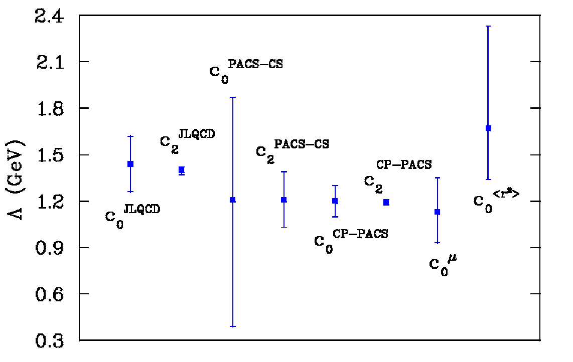
8.2 Future Studies and Further Developments
The research presented in this thesis encourages several avenues for further investigation. In the heavy-baryon formulation of chiral perturbation theory (PT), presented first for the renormalization of the mass of the nucleon in Chapter 4, the finite-volume corrections to the tadpole contribution are not evaluated. This is due to a technical subtlety associated with the large behaviour of the finite-volume correction, due to the coefficient occurring in Equations (4.16) through (4.18). The tadpole finite-volume corrections diverge as . Since it is known that the finite-volume corrections must converge [Bea04b], and lattice QCD simulations do not exhibit any divergence associated with large on a finite volume, higher-order terms, for example, those occurring at order , must act to reduce the estimated value of the finite-volume correction.
In the analysis of the renormalization flow of the nucleon mass, it was discovered that the scale dependence was weakened by working to a sufficiently high chiral order. It was also found, however, that the residual scale-dependence persisted as a significant component of the systematic uncertainty. For efficient propagation of this uncertainty, an interesting future direction would be to consider Bayesian methods of marginalization over the scale-dependence [SP09].
More generally, this research provides a strong basis for the investigation of baryon resonances by analysing lattice QCD simulations. Resonances of the nucleon, such as the Roper Resonance, are not well understood in terms of effective field theory. The structure and behaviour of the resonances lend themselves to a fruitful future area of research. Indeed, it is not possible to link the finite-volume results of lattice QCD to experiment without understanding their relation to the multi-particle states that dress the resonances. FRR EFT is particularly well-suited to exploring this important area of research.
8.3 Codetta
“[T]he collective efforts of numerous physicists have revealed some of nature’s best-kept secrets. And once revealed, these explanatory gems have opened vistas on a world we thought we knew, but whose splendor we had not even come close to imagining.” (Greene, B. 1999. The Elegant Universe p.386) [Gre99]
The dynamics of quantum chromodynamics provide a rich framework for the investigation of the properties of hadrons. In particular, low-energy effective field theory allows one to glean insights into the physical behaviour of subatomic particles and the structure of matter. By incorporating the fundamental symmetries of quantum chromodynamics into the action, chiral perturbation theory provides a robust method for the calculation of hadronic observables within the power-counting regime. In this thesis, finite-range regularized chiral effective field theory was used to develop a procedure for performing calculations beyond the power-counting regime, and handling any subsequent finite-range regularization scale-dependence. Using chiral effective field theory in conjunction with the non-perturbative approach of lattice quantum chromodynamics, chiral extrapolations; finite-volume effects; the consequences of dynamical chiral symmetry breaking on subatomic behaviour; the importance of strangeness; vacuum polarizations; and many other phenomena yield fruitful understanding into the inner workings of the universe.
Concluding Statement
Chiral effective field theory allows the identification of an intrinsic energy scale in the nucleon-pion interaction from lattice simulation results. An optimal finite-range regularization scale, obtained from analyzing the renormalization flow of the low-energy coefficients of the chiral expansion, allows successful extrapolations to be made to the chiral regime and to the infinite-volume limit. There is strong evidence to suggest that the optimal scale characterizes the intrinsic energy scale of the interaction between the pion and the nucleon.
The datum, the results and the rigorous theory integrate to form a strong argument. Chiral effective field theory extended beyond the power counting-regime allows the identification of an intrinsic energy scale, and leads to a robust method for chiral and infinite-volume extrapolations. This is the original contribution of this thesis.
“We have thus achieved the point where the theory may finally be compared with experience, and the road leading from formalism to concrete reality is at last complete.” (Omnès, R. 2002. Quantum Philosophy: Understanding and Interpreting Contemporary Science p.209) [Omn02]
Appendix A Conventions
A.1 Dirac and Pauli Spin Matrices
The Pauli matrices are usually chosen as such:
| (A.1) | ||||
| (A.2) | ||||
| (A.3) |
There are several conventions for the definition of the Dirac matrices (such as Weyl/Chiral or the Majorana Representation). Here is the Dirac Representation:
| (A.4) | ||||
| (A.5) | ||||
| (A.6) |
All representations of these matrices satisfy the requirement of Clifford Algebra due to the conditions imposed in the derivation of the Dirac Equation [Pes95].
| (A.7) | ||||
| (A.8) |
A.2 Gell-Mann Matrices
The generators of the Lie Group satisfy the commutator relations:
| (A.9) |
This, combined with the relevant Jacobi Indentities for the generators, defines the structure constants [Pes95]:
| (A.10) |
A.3 Spinor Fields
The equal-time canonical anti-commutation relations for Dirac spinor fields are:
| (A.11) | ||||
| (A.12) |
The fields take the form [Pes95]:
| (A.13) |
and the canonical anti-commutation relations expressed in terms of the Pauli-Jordan function:
| (A.14) |
The Grassmann algebra is defined by the anticommutation rule between Grassmann variables and a commutation rule with non-Grassmann numbers :
| (A.15) |
For Berezin integration over fermion spinor fields and , the follow rules are adopted:
| (A.16) | ||||
| (A.17) |
where the non-Grassmann constant is chosen, by convention, to be equal to and the function is defined on the Grassmann algebra. As a consequence of Equation (A.17), the Berezin integral over unity vanishes:
| (A.18) |
A.4 Meson and Baryon Field Definitions
The mixed-symmetric meson octet fields can be encoded in a traceless matrix of the form:
| (A.19) |
In the pions form the triplet representation which can be written by summing over the Pauli spin matrices in Appendix (A.1):
| (A.20) |
Using the convention for Clebsch-Gordan coefficients from Wang et al. [WLTY09a], the the mixed-symmetric baryon octet matrix has the form:
| (A.21) |
The maximally symmetric decuplet tensor (suppressing Lorentz indices) has elements defined by:
| (A.22) |
Appendix B Integration Techniques
B.1 Magnetic Quantities
B.1.1 Angular Components of Magnetic Moment Loop Integrals
In anticipation of applying finite-volume corrections to chiral loop integrals by comparing them to their respective summations on the lattice, the time-component of the integral is evaluated using Cauchy’s Integral Formula, and a integral remains for analysis, as in Chapters 4 through 6.
When calculating the magnetic moment in the heavy-baryon limit, without explicitly specifying a regularization scheme, the one-loop integral (corresponding to Figure 7.3) takes the following form:
| (B.1) |
It is useful to be able to simplify the angular part of the integral, formed by the cross product of external momentum direction with the loop momentum , into a numerical coefficient. In order for this to be valid in calculating finite-volume corrections, the simplification must hold in both integral and sum forms of the loop diagram. Evaluating the angular part of Equation (B.1) yields:
| (B.2) | ||||
| (B.3) | ||||
| (B.4) |
Now, this one-dimensional integral can be transformed into a three-dimensional integral simply by adding in a naïve solid angle component, using the identity: :
| (B.5) | ||||
| (B.6) |
Comparing Equations (B.1) and (B.6) shows that the objective has been achieved for the integral case. For finite volume sums, the result may not hold in general, and so must be checked independently. Define the following sum for box length :
| (B.7) |
Because is symmetrical in directions , it follows that:
| (B.8) | ||||
| (B.9) | ||||
| (B.10) |
Thus:
| (B.11) | ||||
| (B.12) |
which is the finite-volume equivalent of Equation (B.6).
B.1.2 Combinatorial Simplification
The calculation of the three-dimensional finite sum can be made more efficient computationally, by transforming it to a one-dimensional sum in terms of the new variable . It does, however, require calculation of the number of configurations of the squares of , and to obtain each value of , denoted . Thus, for an integrand :
| (B.13) |
where .
B.1.3 Sachs Magnetic Form Factors at Finite
Consider calculations involving the leading-order pion loop contributions to the magnetic form factor at finite , (allowing non-zero mass splitting ). The following integral can be made more easily calculable using spherical polar coordinates (using ):
| (B.14) | ||||
| (B.15) |
The integral can be further altered to remove the infinite integral under the change of variables . For arbitrary function :
| (B.16) |
Thus, defining (for convenience) , Equation (B.15) becomes:
| (B.17) |
B.2 Electric Charge Radius Integral Expansions
For the infinite-volume electric charge radius, the chiral loop integrals must be calculated for use with the chiral expansion of Equation (7.27). Each loop integrand is expanded out for small , and the derivative in the limit of vanishing is extracted. Using the notation of Chapter 7, and a dipole regulator, the one-loop contribution takes the following form:
| (B.18) | ||||
| (B.19) |
If a mass-splitting is included:
| (B.20) | ||||
| (B.21) |
Similarly, the tadpole contribution takes the following form:
| (B.22) | ||||
| (B.23) |
B.3 Finite Volume Corrections to Tadpole Amplitudes
Finite-volume corrections should vanish as becomes large, as observed in lattice quantum chromodynamics (lattice QCD) simpulations. This has also been observed, in turn, for each of the finite-volume corrections involved in the extrapolation of the nucleon mass to fourth-order. However, the tadpole finite-volume correction, , is different in that it is multiplied by a factor of , as evident in Equation (4.7). The product is not convergent for large . Figures B.2 and B.2 show the behaviour of the tadpole finite-volume correction for a fm box and a fm box, respectively.


The finite-volume estimate of , denoted , is not in general the same value as the infinite-volume . Thus the finite-volume correction of the tadpole cannot be written as simply the difference between the finite volume sum and the infinite volume integral, but must distinguish between and :
| (B.24) |
Since is by definition the coefficient of the term in the nucleon mass expansion, the renormalization of the residual coefficient by the contributions from the integrals , and , defined in Equations (4.3) through (4.8), can be written as follows:
| (B.25) | ||||
| (B.26) |
An analogous relation exists for the finite volume :
| (B.27) |
By simultaneously solving for and , the ratio can be calculated in principle, and the tadpole finite volume corrections are tractable. It should be noted however, that this does not resolve the problem of divergent behaviour for large .
Appendix C Lattice Simulation Results
| (GeV2) | (GeV) | |
|---|---|---|
| () | ||
| () | ||
| () | ||
| () | ||
| () | ||
| () |
| (GeV2) | (GeV) | |
|---|---|---|
| () | ||
| () | ||
| () | ||
| () | ||
| () |
| (GeV2) | (GeV) | (fm) | (fm) | |
|---|---|---|---|---|
| () | ||||
| () | ||||
| () | ||||
| () | ||||
| () | ||||
| () | ||||
| () | ||||
| () |
| (GeV2) | (GeV) | |
|---|---|---|
| (GeV2) | () | (fm) | (fm) | |
|---|---|---|---|---|
| () | ||||
| () | ||||
| () | ||||
| () | ||||
| () | ||||
| () | ||||
| () | ||||
| () | ||||
| () | ||||
| () |
| (GeV2) | (fm2) | (fm) | (fm) | |
|---|---|---|---|---|
| () | ||||
| () | ||||
| () | ||||
| () | ||||
| () | ||||
| () | ||||
| () |
Bibliography
- [A+05] P. Achard et al. Measurement of the running of the electromagnetic coupling at large momentum-transfer at LEP. Phys.Lett., B623:26–36, 2005.
- [A+09] S. Aoki et al. 2+1 Flavor Lattice QCD toward the Physical Point. Phys.Rev., D79:034503, 2009.
- [AAL+05] C. R. Allton, W. Armour, D. B. Leinweber, A. W. Thomas, and R. D. Young. Chiral and continuum extrapolation of partially-quenched lattice results. Phys. Lett., B628:125–130, 2005.
- [AAL+06] W. Armour, C. R. Allton, D. B. Leinweber, A. W. Thomas, and R. D. Young. Unified chiral analysis of the vector meson spectrum from lattice qcd. J. Phys., G32:971–992, 2006.
- [AK+02] A. Ali Khan et al. Light Hadron Spectroscopy with Two Flavors of Dynamical Quarks on the Lattice. Phys. Rev., D65:054505, 2002.
- [AK+04] A. Ali Khan et al. The nucleon mass in N(f) = 2 lattice QCD: Finite size effects from chiral perturbation theory. Nucl. Phys., B689:175–194, 2004.
- [BCF97] M. Booth, G. Chiladze, and A. F. Falk. Quenched chiral perturbation theory for vector mesons. Phys. Rev., D55:3092–3100, 1997.
- [Bea04a] Silas R. Beane. In search of the chiral regime. Nucl. Phys., B695:192–198, 2004.
- [Bea04b] Silas R. Beane. Nucleon masses and magnetic moments in a finite volume. Phys. Rev., D70:034507, 2004.
- [Ber08] Veronique Bernard. Chiral Perturbation Theory and Baryon Properties. Prog. Part. Nucl. Phys., 60:82–160, 2008.
- [BHLO02] B. Borasoy, B. R. Holstein, R. Lewis, and P. P. A. Ouimet. Long distance regularization in chiral perturbation theory with decuplet fields. Phys. Rev., D66:094020, 2002.
- [BHM04] Veronique Bernard, Thomas R. Hemmert, and Ulf-G. Meissner. Cutoff schemes in chiral perturbation theory and the quark mass expansion of the nucleon mass. Nucl. Phys., A732:149–170, 2004.
- [BM97] B. Borasoy and Ulf-G. Meissner. Chiral expansion of baryon masses and sigma terms. Annals Phys., 254:192–232, 1997.
- [BNS10] Oliver Bar, Silvia Necco, and Andrea Shindler. The epsilon regime with twisted mass Wilson fermions. JHEP, 1004:053, 2010.
- [Boh92] D. Bohm. Thought as a System. Routledge London and New York, 1992.
- [Bor07] Bugra Borasoy. Introduction to Chiral Perturbation Theory. pages 1–26, 2007.
- [CD71] T.P. Cheng and Roger F. Dashen. Is SU(2) x SU(2) a better symmetry than SU(3)? Phys.Rev.Lett., 26:594, 1971.
- [CJJ+74] A. Chodos, R. L. Jaffe, K. Johnson, Charles B. Thorn, and V. F. Weisskopf. A New Extended Model of Hadrons. Phys. Rev., D9:3471–3495, 1974.
- [Col85] S. Coleman. Aspects of Symmetry, Selected Erice Lectures. Cambridge University Press, 1985.
- [CR98] C. K. Chow and S. J. Rey. Quenched and partially quenched chiral perturbation theory for vector and tensor mesons. Nucl. Phys., B528:303–321, 1998.
- [DGH96] J. F. Donahue, E. Golowich, and B. R. Holstein. Dynamics of the Standard Model (Cambridge Monographs on Particle Physics, Nuclear Physics and Cosmology). Cambridge University Press, New Ed Edition, 1996.
- [Dir28a] P.A.M. Dirac. The Quantum theory of electron. 2. Proc.Roy.Soc.Lond., A118:351, 1928.
- [Dir28b] Paul A.M. Dirac. The Quantum theory of electron. Proc.Roy.Soc.Lond., A117:610–624, 1928.
- [DLL96] S. J. Dong, J. F. Lagae, and K. F. Liu. term , in nucleon, and scalar form factor — a lattice study. Phys. Rev., D54:5496–5500, 1996.
- [DSGS05] D. Djukanovic, M. R. Schindler, J. Gegelia, and S. Scherer. Improving the ultraviolet behavior in baryon chiral perturbation theory. Phys. Rev., D72:045002, 2005.
- [Fey39] R. P. Feynman. Forces in Molecules. Phys. Rev., 56:340–343, 1939.
- [FKOU95] M. Fukugita, Y. Kuramashi, M. Okawa, and A. Ukawa. Pion - nucleon sigma term in lattice qcd. Phys. Rev., D51:5319–5322, 1995.
- [G+99] S. Gusken et al. The Pion nucleon sigma term with dynamical Wilson fermions. Phys.Rev., D59:054504, 1999.
- [Gas81] J. Gasser. Hadron Masses and Sigma Commutator in the Light of Chiral Perturbation Theory. Annals Phys., 136:62, 1981.
- [Geo90] Howard Georgi. AN EFFECTIVE FIELD THEORY FOR HEAVY QUARKS AT LOW- ENERGIES. Phys. Lett., B240:447–450, 1990.
- [GHK64] G.S. Guralnik, C.R. Hagen, and T.W.B. Kibble. Global Conservation Laws and Massless Particles. Phys.Rev.Lett., 13:585–587, 1964.
- [GL88] J. Gasser and H. Leutwyler. Spontaneously Broken Symmetries: Effective Lagrangians at Finite Volume. Nucl.Phys., B307:763, 1988.
- [GLS91] J. Gasser, H. Leutwyler, and M.E. Sainio. Sigma term update. Phys.Lett., B253:252–259, 1991.
- [GM64] Murray Gell-Mann. A Schematic Model of Baryons and Mesons. Phys.Lett., 8:214–215, 1964.
- [GML60] Murray Gell-Mann and M Levy. The axial vector current in beta decay. Nuovo Cim., 16:705, 1960.
- [GMOR68] Murray Gell-Mann, R. J. Oakes, and B. Renner. Behavior of current divergences under SU(3) x SU(3). Phys. Rev., 175:2195–2199, 1968.
- [GN74] David J. Gross and Andre Neveu. Dynamical Symmetry Breaking in Asymptotically Free Field Theories. Phys.Rev., D10:3235, 1974.
- [Gre99] B. Greene. The Elegant Universe. Jonathan Cape London, 1999.
- [GSS88] J. Gasser, M. E. Sainio, and A. Svarc. Nucleons with Chiral Loops. Nucl. Phys., B307:779, 1988.
- [GT58] M. L. Goldberger and S. B. Treiman. Decay of the pi meson. Phys. Rev., 110:1178–1184, 1958.
- [Gue66] M. Guenin. On the interaction picture. Communications in Mathematical Physics, 3:120–132, 1966.
- [GW73a] D.J. Gross and Frank Wilczek. Asymptotically Free Gauge Theories. 1. Phys.Rev., D8:3633–3652, 1973.
- [GW73b] D.J. Gross and Frank Wilczek. Ultraviolet Behavior of Nonabelian Gauge Theories. Phys.Rev.Lett., 30:1343–1346, 1973.
- [GW74] D.J. Gross and Frank Wilczek. ASYMPTOTICALLY FREE GAUGE THEORIES. 2. Phys.Rev., D9:980–993, 1974.
- [Haa58] R. Haag. Quantum field theories with composite particles and asymptotic conditions. Phys. Rev., 112:669–673, 1958.
- [Han90] F. C. Hansen. Finite-size effects in spontaneously broken su(n) × su(n) theories. Nuclear Physics B, 345(2-3):685 – 708, 1990.
- [HL90] P. Hasenfratz and H. Leutwyler. Goldstone boson related finite size effects in field theory and critical phenomena with o(n) symmetry. Nuclear Physics B, 343(1):241 – 284, 1990.
- [HL91] F. C. Hansen and H. Leutwyler. Charge correlations and topological susceptibility in qcd. Nuclear Physics B, 350(1-2):201 – 227, 1991.
- [HLY10] J. M. M. Hall, D. B. Leinweber, and R. D. Young. Power Counting Regime of Chiral Effective Field Theory and Beyond. Phys. Rev., D82:034010, 2010.
- [HMRW06] A. Holl, P. Maris, C. D. Roberts, and S. V. Wright. Schwinger functions and light-quark bound states, and sigma terms. Nucl. Phys. Proc. Suppl., 161:87–94, 2006.
- [Höh83] G. Höhler. Pion nucleon scattering. Landolt-Börnstein, 9B2, ed. H. Schopper (Springer) Berlin, 1983.
- [Jen92] Elizabeth Ellen Jenkins. Baryon masses in chiral perturbation theory. Nucl. Phys., B368:190–203, 1992.
- [JLMS93] Elizabeth Ellen Jenkins, Michael E. Luke, Aneesh V. Manohar, and Martin J. Savage. Chiral perturbation theory analysis of the baryon magnetic moments. Phys. Lett., B302:482–490, 1993.
- [JM91a] Elizabeth Ellen Jenkins and Aneesh V. Manohar. Baryon chiral perturbation theory. 1991. Talk presented at the Workshop on Effective Field Theories of the Standard Model, Dobogoko, Hungary, Aug 1991.
- [JM91b] Elizabeth Ellen Jenkins and Aneesh V. Manohar. Baryon chiral perturbation theory using a heavy fermion Lagrangian. Phys. Lett., B255:558–562, 1991.
- [Joh78] K. Johnson. A FIELD THEORY LAGRANGIAN FOR THE MIT BAG MODEL. Phys. Lett., B78:259, 1978.
- [Koc82] R. Koch. Z. Phys., C15:161, 1982.
- [KP80] R. Koch and E. Pietarinen. Nucl. Phys., A336:331, 1980.
- [Leb95] Richard F. Lebed. Determination of SU(6) Clebsch-Gordan coefficients and baryon mass and electromagnetic moment relations. Phys. Rev., D51:5039–5052, 1995.
- [LS96] James N. Labrenz and Stephen R. Sharpe. Quenched chiral perturbation theory for baryons. Phys. Rev., D54:4595–4608, 1996.
- [LSSW96] M. Luscher, S. Sint, R. Sommer, and P. Weisz. Chiral symmetry and o(a) improvement in lattice qcd. Nucl. Phys., B478:365–400, 1996.
- [LTTW00] Derek Bruce Leinweber, Anthony William Thomas, Kazuo Tsushima, and Stewart Victor Wright. Baryon masses from lattice QCD: Beyond the perturbative chiral regime. Phys. Rev., D61:074502, 2000.
- [LTW00] Derek Bruce Leinweber, Anthony William Thomas, and Stewart Victor Wright. Lattice QCD calculations of the sigma commutator. Phys. Lett., B482:109–113, 2000.
- [LTY04] Derek Bruce Leinweber, Anthony William Thomas, and Ross Daniel Young. Physical nucleon properties from lattice QCD. Phys. Rev. Lett., 92:242002, 2004.
- [LTY05] D. B. Leinweber, A. W. Thomas, and R. D. Young. Extrapolation of lattice qcd results beyond the power- counting regime. Nucl. Phys., A755:59–70, 2005.
- [LTY06] D. B. Leinweber, A. W. Thomas, and R. D. Young. Power counting regime of chiral extrapolation and beyond. PoS, LAT2005:048, 2006.
- [Lub97] M. Lublinsky. g(omega rho pi) reexamined. Phys. Rev., D55:249–254, 1997.
- [MB99] Judith A. McGovern and Michael C. Birse. On the absence of fifth-order contributions to the nucleon mass in heavy-baryon chiral perturbation theory. Phys. Lett., B446:300–305, 1999.
- [MB06] Judith A. McGovern and Michael C. Birse. Convergence of the chiral expansion for the nucleon mass. Phys. Rev., D74:097501, 2006.
- [MG84] Aneesh Manohar and Howard Georgi. Chiral Quarks and the Nonrelativistic Quark Model. Nucl. Phys., B234:189, 1984.
- [MTT80] Gerald A. Miller, Anthony William Thomas, and S. Theberge. Pion - Nucleon Scattering in the Cloudy Bag Model. Phys. Lett., B91:192, 1980.
- [NK87] Ann E. Nelson and David B. Kaplan. Strange Condensate Realignment in Relativistic Heavy Ion Collisions. Phys.Lett., B192:193, 1987.
- [NN95] R. Narayanan and H. Neuberger. A construction of lattice chiral gauge theories. Nucl. Phys., B443:305–385, 1995.
- [O+08] H. Ohki et al. Nucleon sigma term and strange quark content from lattice QCD with exact chiral symmetry. Phys. Rev., D78:054502, 2008.
- [Omn02] R. Omnès. Quantum Philosophy: Understanding and Interpreting Contemporary Science. Princeton University Press, 2002.
- [Pes95] D. V. Peskin, M. E. Schroeder. An Introduction to Quantum Field Theory. Perseus Books Publishing L.L.C., 1995.
- [Pol73] H.David Politzer. Reliable Perturbative Results for Strong Interactions? Phys.Rev.Lett., 30:1346–1349, 1973.
- [Pro96] Serban Protopopescu. Observation of the Top Quark. Nuovo Cim., A109:755–769, 1996.
- [PSWA02] M.M. Pavan, I.I. Strakovsky, R.L. Workman, and R.A. Arndt. The Pion nucleon Sigma term is definitely large: Results from a G.W.U. analysis of pi nucleon scattering data. PiN Newslett., 16:110–115, 2002.
- [RCR10] H.L.L. Roberts, L. Chang, and C.D. Roberts. Impact of dynamical chiral symmetry breaking on meson structure and interactions. 2010.
- [RS80] M. Reed and B. Simon. Methods of Modern Mathematical Physics, Vol 1: Functional Analysis. Academic Press, 1980.
- [RW94] Craig D. Roberts and Anthony G. Williams. Dyson-Schwinger equations and their application to hadronic physics. Prog.Part.Nucl.Phys., 33:477–575, 1994.
- [SDGS07] M. R. Schindler, D. Djukanovic, J. Gegelia, and S. Scherer. Chiral expansion of the nucleon mass to order O(q**6). Phys. Lett., B649:390–393, 2007.
- [Sha97] Stephen R. Sharpe. Chiral perturbation theory and weak matrix elements. Nucl. Phys. Proc. Suppl., 53:181–198, 1997.
- [SP09] Matthias R. Schindler and Daniel R. Phillips. Bayesian Methods for Parameter Estimation in Effective Field Theories. Annals Phys., 324:682–708, 2009.
- [SS05] Stefan Scherer and Matthias R. Schindler. A Chiral perturbation theory primer. 2005.
- [SW85] B. Sheikholeslami and R. Wohlert. Improved continuum limit lattice action for qcd with wilson fermions. Nucl. Phys., B259:572, 1985.
- [tHV72] G. ’t Hooft and M. J. G. Veltman. Regularization and renormalization of gauge fields. Nucl. Phys., B44:189–213, 1972.
- [VW84] C. Vafa and Edward Witten. Restrictions on Symmetry Breaking in Vector-Like Gauge Theories. Nucl. Phys., B234:173, 1984.
- [Wei95] S. Weinberg. The Quantum Theory of Fields. Cambridge University Press, 1995.
- [Wil74] Kenneth G. Wilson. Confinement of Quarks. Phys.Rev., D10:2445–2459, 1974.
- [WL05] Andre Walker-Loud. Octet baryon masses in partially quenched chiral perturbation theory. Nucl. Phys., A747:476–507, 2005.
- [WLT00] Stewart Victor Wright, Derek Bruce Leinweber, and Anthony William Thomas. The sigma commutator from lattice QCD. Nucl. Phys., A680:137–140, 2000.
- [WLTY07] P. Wang, Derek Bruce Leinweber, Anthony William Thomas, and Ross Daniel Young. Chiral extrapolation of nucleon magnetic form factors. Phys. Rev., D75:073012, 2007.
- [WLTY09a] P. Wang, D.B. Leinweber, A.W. Thomas, and R.D. Young. Chiral extrapolation of octet-baryon charge radii. Phys.Rev., D79:094001, 2009.
- [WLTY09b] P. Wang, D.B. Leinweber, A.W. Thomas, and R.D. Young. Strange magnetic form factor of the proton at Q**2 = 0.23- GeV**2. Phys.Rev., C79:065202, 2009.
- [Y+06] W. M. Yao et al. Review of particle physics. J. Phys., G33:1–1232, 2006.
- [YHL09] Ross D. Young, Jonathan M. M. Hall, and Derek B. Leinweber. Towards selecting a finite-range regularization scale. 2009.
- [YLT03] R. D. Young, D. B. Leinweber, and A. W. Thomas. Convergence of chiral effective field theory. Prog. Part. Nucl. Phys., 50:399–417, 2003.
- [YT10a] R.D. Young and A.W. Thomas. Octet baryon masses and sigma terms from an SU(3) chiral extrapolation. Phys.Rev., D81:014503, 2010.
- [YT10b] Ross D. Young and Anthony W. Thomas. Recent results on nucleon sigma terms in lattice QCD. Nucl.Phys., A844:266C–271C, 2010.
- [Z+02] J. M. Zanotti et al. Hadron masses from novel fat-link fermion actions. Phys. Rev., D65:074507, 2002.