KP solitons, higher Bruhat and Tamari orders

Waves on a fluid surface show a very complex behavior in general. Only under special circumstances can we expect to observe a more regular pattern. For shallow water waves, the Kadomtsev-Petviashvili (KP) equation

$\displaystyle(-4\,u_{t}+u_{xxx}+6\,uu_{x})_{x}+3\,u_{yy}=0$

(where e.g. $u_{t}=\partial u/\partial t$) provides an approximation under the conditions that the wave dominantly travels in the $x$-direction, the wave length is long as compared with the water depth, and the effect of the nonlinearity is about the same order as that of dispersion.¹¹ 1 The physical form of this equation is obtained by suitable rescalings of $x,y,t$ and $u$, involving physical parameters. More precisely, this is the KP-II equation, but we will write KP, for short. It generalizes the famous Korteweg-deVries (KdV) equation, which describes waves moving in only one spatial dimension. Although the KdV equation is much better established as an approximation of the more general water wave equations, recent studies also confirm the physical relevance of KP [9].

In [2] we studied the soliton solutions of the KP equation in a tropical approximation, which reduces them to networks formed by line segments in the $xy$-plane, evolving in time $t$. A subclass corresponds to evolutions (in time $t$) in the set of (planar) rooted binary trees. At transition events, the binary tree type changes (through a tree that is not binary). It turned out that the time evolution is simply given by right rotation in a tree, and the solution evolves according to a maximal chain of a Tamari lattice [24, 25], see Figure 1.

In this realization of Tamari lattices, the underlying set consists of states of a physical system, here the tree-types of a soliton configuration in the $xy$-plane. The Tamari poset (partially ordered set) structure describes the possible ways in which these states are allowed to evolve in time, starting from an initial state (the top node) and ending in a final state (the bottom node).

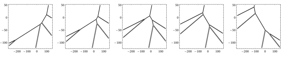
Figure 2 displays a solution evolving via a tree rotation, and further provides an idea how this can be understood in terms of an arrangement of planes in three-dimensional space-time (after idealizing line soliton branches to lines in the $xy$-plane, see Section 3).

In this work we show that the classification of possible evolutions of tree-shaped KP line solitons involves higher Bruhat orders [17, 18, 19, 30]. Moreover, we are led to associate with each higher Bruhat order a higher Tamari order via a surjection, in a way different from what has been considered previously. There is some evidence that our higher Tamari orders coincide with ‘higher Stasheff-Tamari posets’ introduced by Kapranov and Voevodsky [8] (also see [3]), but a closer comparison will not be undertaken in this work.

In Section 2, we briefly describe the general class of KP soliton solutions. In Section 3, we concentrate on the abovementioned subclass of tree-shaped solutions, in the tropical approximation, and somewhat improve results in [2]. Section 4 recalls results about higher Bruhat orders and extracts from the analysis of tree-shaped KP line solitons a reduction to higher Tamari orders. Section 7 proposes a hierarchy of monoids that expresses the hierarchical structure present in the KP soliton problem. This makes contact with simplex equations [29, 1, 6, 13] and provides us with an algebraic method to construct higher Bruhat and higher Tamari orders. Section 8 contains some additional remarks. Throughout this work, Hasse diagrams of posets will be displayed upside down (i.e. with the lowest element(s) at the top).

The line soliton solutions of the KP-II equation are parametrized by the totally non-negative Grassmannians $\mathrm{Gr}^{\geq}_{n,M+1}$ [9], which is easily recognized in the Wronskian form of the solutions. Translating the KP equation via

$\displaystyle u=2\,\log(\tau)_{xx}\,,$

into a bilinear equation in the variable $\tau$, these solutions are given by

$\displaystyle\tau=f_{1}\wedge f_{2}\wedge\cdots\wedge f_{n}\,,$

where

$\displaystyle f_{i}=\sum_{j=1}^{M+1}a_{ij}\;e_{j}\,,\qquad e_{j}=e^{\theta_{j}}\,,\qquad\theta_{j}=\sum_{r=1}^{M}p_{j}^{r}\;t^{(r)}+c_{j}\;.$

Here $t^{(r)}$, $r=1,\ldots,M$, are independent real variables that may be regarded as coordinates on $\mathbb{R}^{M}$, and we set $t^{(1)}=x$, $t^{(2)}=y$, $t^{(3)}=t$. The variables $t^{(r)}$, $r>3$, are the additional evolution variables that appear in the KP hierarchy, which extends the KP equation to an infinite set of compatible PDEs. Furthermore, $p_{j},c_{j},a_{ij}$ are real constants, and without restriction of generality we can and will assume that

$\displaystyle p_{1}<p_{2}<\cdots<p_{M+1}\;.$

The exterior product on the space of functions generated by the exponential functions $e_{j}$, $j=1,\ldots,M+1$, is defined by

$\displaystyle e_{i_{1}}\wedge\cdots\wedge e_{i_{m}}=\Delta(p_{i_{1}},\ldots,p_{i_{m}})\,e_{i_{1}}\cdots e_{i_{m}}\,,$

with the Vandermonde determinant

$\displaystyle\Delta(p_{i_{1}},\ldots,p_{i_{m}})=\left|\begin{array}[]{cccc}1&p_{i_{1}}&\cdots&p_{i_{1}}^{m-1}\\ 1&p_{i_{2}}&\cdots&p_{i_{2}}^{m-1}\\ \vdots&\vdots&\cdots&\vdots\\ 1&p_{i_{m}}&\cdots&p_{i_{m}}^{m-1}\end{array}\right|=\prod_{1\leq r<s\leq m}(p_{i_{s}}-p_{i_{r}})\;.$

Now we can express $\tau$ as

$\displaystyle\tau=\sum_{I\in{[M+1]\choose n}}A_{I}\,\Delta(p_{I})\,e_{I}\,,$

where $[m]=\{1,2,\ldots,m\}$, and ${[m]\choose n}$ denotes the set of $n$-element subsets of $[m]$. Numbering the elements of a subset $I=\{i_{1},\ldots,i_{n}\}$ such that $i_{1}<\cdots<i_{n}$, we set $\Delta(p_{I})=\Delta(p_{i_{1}},\ldots,p_{i_{n}})$. Finally, $A_{I}$ denotes the maximal minor with columns $i_{1},\ldots,i_{n}$ of the matrix

$\displaystyle A=\left(\begin{array}[]{ccc}a_{1,1}&\cdots&a_{1,M+1}\\ \vdots&\ddots&\vdots\\ a_{n,1}&\cdots&a_{n,M+1}\end{array}\right)\;.$

For regular (soliton) solutions, the Plücker coordinates $A_{I}$ have to be non-negative real numbers (and at least one has to be different from zero). In the following we concentrate on the subclass of solutions parametrized by $\mathrm{Gr}^{\geq}_{1,M+1}$, i.e.

$\displaystyle\tau=e_{1}+\cdots+e_{M+1}\,,$

(3)

where we absorbed the positive constants $a_{1,j}$ into the constants $c_{j}$. To good approximation, a general line soliton solution can be understood as a superimposition of solutions from the subclass (see [2]).

Let us fix $M\in\mathbb{N}$, constants $p_{1}<p_{2}<\cdots<p_{M+1}$ and $c_{i}$, $i=1,\ldots,M+1$. The behavior of $\tau\,:\,\mathbb{R}^{M}\to\mathbb{R}$, given by (3), is best understood in a tropical approximation of $\log(\tau)$. In a region where some phase, say $\theta_{i}$, dominates all others, i.e. $\theta_{i}>\theta_{j}$ for all $j\neq i$, we have

$\displaystyle\log(\tau)=\theta_{i}+\log\Big(1+\sum_{j=1\atop j\neq i}^{M+1}e^{-(\theta_{i}-\theta_{j})}\Big)\simeq\theta_{i}\;.$

As a consequence,

$\displaystyle\log(\tau)\simeq\max\{\theta_{1},\ldots,\theta_{M+1}\}\,,$

where the right hand side can be regarded as a tropical version of $\log(\tau)$. Sufficiently away from the boundary of a dominating-phase region, $\log(\tau)$ is linear in $x$, so that $u$ vanishes. A crucial observation is that a line soliton branch in the $xy$-plane, for fixed $t^{(r)}$, $r>2$, corresponds to a boundary line between two dominating-phase regions. Viewing it in space-time, by regarding $t$ as a coordinate of an additional dimension, or more generally in the extended space $\mathbb{R}^{M}$ by adding dimensions corresponding to the evolution variables $t^{(r)}$, $r=3,\ldots,M$, the boundary consists piecewise of affine hyperplanes. Let $\mathcal{U}_{i}$ denote the region where $\theta_{i}$ is not dominated by any other phase, i.e.

$\displaystyle\mathcal{U}_{i}=\{\mathbf{t}\in\mathbb{R}^{M}\,|\,\max\{\theta_{1},\ldots,\theta_{M+1}\}=\theta_{i}\}=\bigcap_{k\neq i}\{\mathbf{t}\in\mathbb{R}^{M}\,|\,\theta_{k}\leq\theta_{i}\}\;.$

(4)

In the tropical approximation, a description of KP line solitons amounts to an analysis of intersections of such regions, i.e.

$\displaystyle\mathcal{U}_{I}=\mathcal{U}_{i_{1}}\cap\cdots\cap\mathcal{U}_{i_{n}}\,,\quad I=\{i_{1},\ldots,i_{n}\}\in{\Omega\choose n}\,,\quad\Omega:=[M+1]=\{1,\ldots,M+1\}\;.$

This is a subset of the affine space

$\displaystyle\mathcal{P}_{I}=\{\mathbf{t}\in\mathbb{R}^{M}\,|\,\theta_{i_{1}}=\cdots=\theta_{i_{n}}\}\qquad\qquad n>1\,,$

which is easy to deal with (see below). It is more difficult to determine which parts of $\mathcal{P}_{I}$ are visible, i.e. belong to $\mathcal{U}_{I}$. Fixing the values of $t^{(r)}$, $r>2$, determines a line soliton segment in the $xy$-plane if $n=2$, and a meeting point of $n$ such segments if $n>2$.²² 2 For generic values of $t^{(r)}$, $r>2$, we see line soliton segments and meeting points of three segments in the $xy$-plane. Meeting points of more than three segments only occur for special values. In order to decide about visibility, i.e. whether a point of $\mathcal{P}_{I}$ lies in $\mathcal{U}_{I}$, a formula is needed to compare the values of all phases at this point, see (12) below.

Let us first look at $\mathcal{P}_{I}$ in more detail. Introducing a real auxiliary variable $t^{(0)}$, the equation $\theta_{i_{1}}=\cdots=\theta_{i_{n}}=-t^{(0)}$ results in the linear system³³ 3 We note that the full set of equations $t^{(0)}+p_{i}\,t^{(1)}+p_{i}^{2}\,t^{(2)}+\cdots+p_{i}^{M}\,t^{(M)}=-c_{i}$, $i=1,\ldots,M+1$, defines a cyclic hyperplane arrangement [30] in $\mathbb{R}^{M+1}$ with coordinates $t^{(0)},\ldots,t^{(M)}$.

$\displaystyle t^{(0)}+p_{i_{j}}\,t^{(1)}+p_{i_{j}}^{2}\,t^{(2)}+\cdots+p_{i_{j}}^{n-1}\,t^{(n-1)}=-\tilde{c}_{i_{j}}\,,\qquad j=1,\ldots,n\,,$

where

$\displaystyle\tilde{c}_{i_{j}}=c_{i_{j}}+p_{i_{j}}^{n}\,t^{(n)}+\cdots+p_{i_{j}}^{M}\,t^{(M)}\;.$

This fixes the first $n-1$ coordinates as linear functions of the remaining coordinates, $t_{I}^{(k)}=t_{I}^{(k)}(t^{(n)},\ldots,t^{(M)})$, $k=1,\ldots,n-1$. In particular, we obtain (also see [2], Appendix A)

	$\displaystyle t_{I}^{(n-1)}$	$\displaystyle=$	$\displaystyle-\sum_{r=1}^{M+1-n}h_{r}(p_{I})\,t^{(n+r-1)}-c_{I}$		(5)
		$\displaystyle=$	$\displaystyle-(p_{i_{1}}+\cdots+p_{i_{n}})\,t^{(n)}-\tilde{c}_{I}\,,$

where $h_{r}(p_{I})=h_{r}(p_{i_{1}},\ldots,p_{i_{n}})$ is the $r$-th complete symmetric polynomial [15] in the variables $p_{i_{1}},\ldots,p_{i_{n}}$, and

$\displaystyle c_{I}=\frac{1}{\Delta(p_{I})}\sum_{s=1}^{n}(-1)^{n-s}\,c_{i_{s}}\,\Delta(p_{I\setminus\{i_{s}\}})\,,\qquad\tilde{c}_{I}=\sum_{r=2}^{M+1-n}h_{r}(p_{I})\,t^{(n+r-1)}+c_{I}\;.$

We note that $\tilde{c}_{I}$ depends on $t^{(n+1)},\ldots,t^{(M)}$. Here are some immediate consequences:

• •

  Since obviously $\mathcal{P}_{I}\subset\mathcal{P}_{J}$ for $J\subset I$, on $\mathcal{P}_{I}$ we have

  $\displaystyle t_{I}^{(n-2)}=t_{I\setminus\{i_{n}\}}^{(n-2)}(t_{I}^{(n-1)},t^{(n)},\ldots,t^{(M)})\,,$

  and corresponding expressions for $t_{I}^{(r)}$, $r=1,\ldots,n-3$.

• •

  $\mathcal{P}_{\Omega}$ is a common point of all $\mathcal{P}_{I}$, $I\subset\Omega$. According to (5), on $\mathcal{P}_{\Omega}$ we have

  $\displaystyle t_{\Omega}^{(M)}=-c_{\Omega}\;.$

  Clearly, $\mathcal{P}_{\Omega}=\mathcal{U}_{\Omega}$, and is thus visible.

• •

  The hyperplane $\mathcal{P}_{\{i_{1},i_{2}\}}$ is given by

  $\displaystyle t^{(1)}_{\{i_{1},i_{2}\}}=-(p_{i_{1}}+p_{i_{2}})\,t^{(2)}-\tilde{c}_{\{i_{1},i_{2}\}}\,,$

  and we have

  $\displaystyle\theta_{i_{2}}-\theta_{i_{1}}=(p_{i_{2}}-p_{i_{1}})\,(t^{(1)}-t^{(1)}_{\{i_{1},i_{2}\}})\,,$

  (6)

  so that, for $i_{1}<i_{2}$,

  $\displaystyle t^{(1)}\lessgtr t^{(1)}_{\{i_{1},i_{2}\}}\quad\Longleftrightarrow\quad\theta_{i_{2}}\lessgtr\theta_{i_{1}}\;.$

  Together with (4), this implies in particular that each $\mathcal{U}_{i}$ is the intersection of half-spaces, and thus a closed convex set. None of these sets is empty since they all contain $\mathcal{U}_{\Omega}$. It follows in turn that each set $\mathcal{U}_{I}$ (with non-empty $I$) is non-empty, closed and convex (and thus in particular connected).

With the help of this important lemma, we obtain the following result.

The first chain in (3.2) is in lexicographic order, the second in reverse lexicographic order, with respect to the index sets. This makes contact with higher Bruhat orders, see Section 4. The following result is crucial for determining (non-)visible events.

For $k\leq l$, let $[k,l]$ denote the interval $\{k,k+1,\ldots,l\}$. We call an interval even (respectively odd) if its cardinality is even (respectively odd). Now we formulate a generalization of results in Example 3.4. The proof is by inspection of (12), which depends on the structure of $I$. We note that an even interval cannot influence the sign of the right hand side of (12).

In the following, $K$ denotes the set $\{k_{1},\ldots,k_{n+1}\}$, and will be assumed to be in linear order, so that $k_{1}<\cdots<k_{n+1}$. We split such a set into⁵⁵ 5 $\lceil n/2\rceil$ denotes the smallest integer greater than or equal to $n/2$, and $\lfloor n/2\rfloor$ the largest integer smaller than or equal to $n/2$.

	$\displaystyle K_{<}=\{k_{n-2r}\,|\,r=0,\ldots,\lceil n/2\rceil-1\}=\{k_{2-(n\,\mathrm{mod}\,2)},\ldots,k_{n}\}\,,$
	$\displaystyle K_{>}=\{k_{n-2r+1}\,|\,r=0,\ldots,\lfloor n/2\rfloor\}=\{k_{1+(n\,\mathrm{mod}\,2)},\ldots,k_{n+1}\}\;.$

Choosing a point $\mathbf{t}_{0}\in\mathcal{P}_{K}$ means fixing the free coordinates on $\mathcal{P}_{K}$ to values $t^{(n+1)}_{0},\ldots,t^{(M)}_{0}$. For each $k\in K$, it determines a line

$\displaystyle\{\mathbf{t}_{K\setminus\{k\}}(\lambda,t^{(n+1)}_{0},\ldots,t^{(M)}_{0})\,|\,\lambda\in\mathbb{R}\}\subset\mathcal{P}_{K\setminus\{k\}}\;.$

According to Proposition 3.9, Proposition 3.8 provides us with a method to determine all non-visible points, and thus also all visible points.

A point $\mathbf{t}_{0}\in\mathcal{P}_{I}$ is called generic if $\mathbf{t}_{0}\notin\mathcal{P}_{J}$ for every $J\subset\Omega$ , $J\not\subset I$.

Now we arrived at the following situation. From Proposition 3.2, we recall that

$\displaystyle\begin{array}[]{l}t^{(n-1)}_{K\setminus\{k_{n+1}\}}<t^{(n-1)}_{K\setminus\{k_{n-1}\}}<\cdots<t^{(n-1)}_{K\setminus\{k_{1+(n\,\mathrm{mod}\,2)}\}}\\[8.61108pt] t^{(n-1)}_{K\setminus\{k_{2-(n\,\mathrm{mod}\,2)}\}}<\cdots<t^{(n-1)}_{K\setminus\{k_{n-2}\}}<t^{(n-1)}_{K\setminus\{k_{n}\}}\end{array}\quad\mbox{for}\quad\begin{array}[]{l}t^{(n)}<t^{(n)}_{K}\\[8.61108pt] t^{(n)}>t^{(n)}_{K}\;.\end{array}$

For all $t^{(n-1)}_{K\setminus\{k_{i}\}}$ that are absent in the respective chain, there is no visible event in the respective half-space ($t^{(n)}<t^{(n)}_{K}$, respectively $t^{(n)}>t^{(n)}_{K}$). Let $\mathbf{t}_{0}\in\mathcal{P}_{K}$ be given by $t^{(n)}=t^{(n)}_{K}$ and fixing the higher variables to $t^{(n+1)}_{0},\ldots,t^{(M)}_{0}$. Let $\mathbf{t}_{0}$ be visible and generic, and $t^{(n-1)}_{K\setminus\{k_{i}\}}$ in one of the chains in (3). For $t^{(n)}$ close enough to $t^{(n)}_{K}$, and on the respective side according to (3), every event in $\mathcal{P}_{K\setminus\{k_{i}\}}$ with remaining coordinates $t^{(n)},t^{(n+1)}_{0},\ldots,t^{(M)}_{0}$ is visible.

We described line solitons as objects moving in the $xy$-plane (where $x=t^{(1)}$ and $y=t^{(2)}$). They evolve according to the KP equation (with evolution parameter $t=t^{(3)}$), the first equation of the KP hierarchy. A higher KP hierarchy equation has one of the parameters $t^{(r)}$, $r>3$, as its evolution parameter. We do not consider the corresponding evolutions in this work, but it turned out that these parameters are important in order to classify the various evolutions. We showed that solitons from a subclass have the form of rooted binary trees with leaves extending to infinity in the $xy$-plane and evolving by right rotation as time $t$ proceeds. They all start with the same asymptotic form as $t\sim-\infty$ and end with the same asymptotic form as $t\sim+\infty$. These are the maximal and minimal element, respectively, of a Tamari lattice, and any generic evolution thus corresponds to a maximal chain. For a soliton configuration with $M+1$ leaves, which chain is realized depends on the values of the parameters $t^{(r)}$, $r=1,\ldots,M$.

According to Proposition 3.2, a substantial role in the combinatorics underlying the tree-shaped line solitons is played by the order relations (3.2). They are at the roots of the generalization by Manin and Schechtman of the weak Bruhat order on the set of permutations of $[m]$ to ‘higher Bruhat orders’ [17, 18, 19], also see [30]. In the following subsection we recall some definitions and results mainly from [30]. In section 4.2 we introduce ‘higher Tamari orders’.

References

• [1] V. Bazhanov and Y. Stroganov, “Conditions of commutativity of transfer matrices on a multidimensional lattice”, Theor. Math. Phys. 52 (1982) 685–691.
• [2] A. Dimakis and F. Müller-Hoissen, “KP line solitons and Tamari lattices”, J. Phys. A: Math. Theor. 44 (2011) 025203.
• [3] P. Edelman and V. Reiner, “The higher Tamari posets”, Mathematika 43 (1996) 127–154.
• [4] S. Felsner and H. Weil, “A theorem on higher Bruhat orders”, Discr. Comput. Geom. 23 (2000) 121–127.
• [5] S. Felsner and G. Ziegler, “Zonotopes associated with higher Bruhat orders”, Discr. Math. 241 (2001) 301–312.
• [6] I. Frenkel and G. Moore, “Simplex equations and their solutions”, Commun. Math. Phys. 138 (1991) 259–271.
• [7] J. Hietarinta and F. Nijhoff, “The eight tetrahedron equations”, J. Math. Phys. 38 (1997) 3603–3615.
• [8] M. Kapranov and V. Voevodsky, “Combinatorial-geometric aspects of polycategory theory: pasting schemes and higher bruhat orders (list of results)”, Cahiers de topologie et géométrie différentielle catégoriques 32 (1991) 11–27.
• [9] Y. Kodama, “KP solitons in shallow water”, J. Phys. A: Math. Theor. 43 (2010) 434004.
• [10] I. Korepanov, “Tetrahedral Zamolodchikov algebras corresponding to Baxter’s LL-operators”, Comm. Math. Phys. 154 (1993) 85–97.
• [11]   , “The tetrahedron equation and algebraic geometry”, J. Math. Sci. 83 (1997) 85–92.
• [12] R. Lawrence, “Algebras and triangle relations”, J. Pure Appl. Alg. 100 (1995) 43–72.
• [13]   , “Yang-Baxter type equations and posets of maximal chains”, J. Comb. Theory, Ser. A 79 (1997) 68–104.
• [14] J.-L. Loday, “Dichotomy of the addition of natural numbers”, arXiv:1108.6238v1 [math.RA], to appear in the Tamari Memorial Festschrift.
• [15] I. Macdonald, Symmetric functions and Hall polynomials, 2nd ed., Oxford University Press, Oxford, 1995.
• [16] J. Maillet and F. Nijhoff, “Multidimensional latttice integrability and the simplex equations”, in Nonlinear Evolution Equations: Integrability and Spectral Methods, A. Degasperis, A. Fordy, and M. Lakshmanan, eds., Manchester University Press, 1990, 537–548.
• [17] Y. Manin and V. Schechtman, “Arrangements of real hyperplanes and Zamolodchikov equations”, in Group Theoretical Methods in Physics, M. Markov, V. Man’ko, and V. Dodonov, eds., Adv. Stud. Pure Math., vol. 17, VNU Science Press, 1986, 151–165.
• [18]   , “Higher Bruhat orders, related to the symmetric group”, Funct. Anal. Appl. 20 (1986) 148–150.
• [19]   , “Arrangements of hyperplanes, higher braid groups and higher Bruhat orders”, in Algebraic Number Theory – in honor of K. Iwasawa, J. Coates, R. Greenberg, B. Mazur, and I. Satake, eds., Adv. Stud. Pure Math., vol. 17, Academic Press, 1989, 289–308.
• [20] F. Michielsen and F. Nijhoff, “D-algebras, the D-simplex equations, and multidimensional integrability”, in Quantum Topology, L. Kauffman and R. Baadhio, eds., Series on Knots and Everything, vol. 3, World Scientific, 1993, 230–243.
• [21] J. Perk and H. Au-Yang, “Yang-Baxter equations”, in Encyclopedia of Mathematical Physics, J.-P. Françoise, G. Naber, and S. Tsou, eds., vol. 5, Elsevier Science, 2006, 465–473.
• [22] J. Rambau and V. Reiner, “A survey of the higher Stasheff-Tamari orders”, preprint, to appear in the Tamari Memorial Festschrift.
• [23] R. Street, “The algebra of oriented simplexes”, J. Pure Appl. Alg. 49 (1987) 283–335.
• [24] D. Tamari, “Monoides préordonnés et chaînes de Malcev”, Doctorat ès-Sciences Mathématiques Thèse de Mathématique, Paris, 1951.
• [25]   , “The algebra of bracketings and their enumeration”, Nieuw Arch. Wisk. 10 (1962) 131–146.
• [26] H. Thomas, “Maps between higher Bruhat orders and higher Stasheff-Tamari posets”, in FPSAC 15th Anniversary International Conference on Formal Power Series and Algebraic Combinatorics, K. Eriksson, A. Björner, and S. Linusson, eds., 2003.
• [27] M. Voevodski and M. Kapranov, “Free nn-categories generated by a cube, oriented matroids, and higher Bruhat orders”, Funct. Anal. Appl. 25 (1990) 50–52.
• [28] Wolfram Research, Inc., Mathematica 8.0, Wolfram Research, Inc., Champaign, Illinois, 2010.
• [29] A. Zamolodchikov, “Tetrahedron equations and the relativistic SS-matrix of straight-strings in 2+1-dimensions”, Commun. Math. Phys. 79 (1981) 489–505.
• [30] G. Ziegler, “Higher Bruhat orders and cyclic hyperplane arrangements”, Topology 32 (1993) 259–297.