Modular curvature for noncommutative two-toriThanks: The work of the first named author was partially supported by the National Science Foundation award no. DMS-0652164Thanks: The work of the second named author was partially supported by the National Science Foundation award no. DMS-0969672

Alain Connes Address: A. Connes: Collège de France
3, rue d’Ulm
Paris, F-75005 France
I.H.E.S. and Vanderbilt University Email address: alain@connes.org and Henri Moscovici Address: H. Moscovici: Department of mathematics, The Ohio State University, Columbus, OH 43210, USA Email address: henri@math.ohio-state.edu

Abstract.

In this paper we investigate the curvature of conformal deformations by noncommutative Weyl factors of a flat metric on a noncommutative 2-torus, by analyzing in the framework of spectral triples functionals associated to perturbed Dolbeault operators. The analogue of Gaussian curvature turns out to be a sum of two functions in the modular operator corresponding to the non-tracial weight defined by the conformal factor, applied to expressions involving the derivatives of the same factor. The first is a generating function for the Bernoulli numbers and is applied to the noncommutative Laplacian of the conformal factor, while the second is a two-variable function and is applied to a quadratic form in the first derivatives of the factor. Further outcomes of the paper include a variational proof of the Gauss-Bonnet theorem for noncommutative 2-tori, the modular analogue of Polyakov’s conformal anomaly formula for regularized determinants of Laplacians, a conceptual understanding of the modular curvature as gradient of the Ray-Singer analytic torsion, and the proof using operator positivity that the scale invariant version of the latter assumes its extreme value only at the flat metric.

Introduction

In noncommutative geometry the paradigm of a geometric space is given in spectral terms, by a Hilbert space ${\mathcal{H}}$ in which both the algebra ${\mathcal{A}}$ of coordinates and the analogue of the inverse line element $ds^{-1}$ are represented, the latter being embodied by an unbounded self-adjoint operator $D$ which plays the role of the Dirac operator. The local geometric invariants such as the Riemannian curvature are extracted from the functionals defined by the coefficients of heat kernel expansion

{\rm Tr}(ae^{-tD^{2}})\,\sim_{t\searrow 0}\,\sum_{n\geq 0}{\rm a}_{n}(a,D^{2})t^{\frac{-d+n}{2}}\,,\quad a\in{\mathcal{A}},

where $d$ is the dimension of the geometry. Equivalently, one may consider special values of the corresponding zeta functions. Thus, it is the high frequency behavior of the spectrum of $D$ coupled with the action of the algebra ${\mathcal{A}}$ in ${\mathcal{H}}$ which detects the local curvature of the geometry.

In this paper we implement the Riemannian aspect of this program in great depth on an archetypal example, that of the noncommutative two torus ${\rm T}^{2}_{\theta}$ , whose differential geometry as well as pseudo-differential operator calculus were first developed in [8]. To obtain a curved geometry from the flat one defined in [8], one introduces (cf. [7], [13]) a noncommutative Weyl conformal factor (or dilaton), which changes the metric by modifying the noncommutative volume form while keeping the same conformal structure. Both notions of volume form and of conformal structure are well understood in the general case (cf. [9, §VI]). We recall in §1 how one obtains the modified Dirac operator for the curved geometry obtained from a flat one by modifying the volume form.

The starting point is the computation of the value at $s=0$ of the zeta function ${\rm Tr}(a|D|^{-2s})$ for the $2$ -dimensional curved geometry associated to the dilaton $h$ , or equivalently of the coefficient ${\rm a}_{2}(a,D^{2})$ of the heat expansion. This computation was initiated in the late 1980’s (cf. [7]), and the specific result which proves the analogue of the Gauss–Bonnet formula was published in [13]. It was subsequently extended in [14] to the case of arbitrary values of the complex modulus $\tau$ (set to $\tau=i$ in [13]). In both these papers only the total integral of the curvature was needed, and this allowed one to make simplifications under the trace which are no longer possible when $a\neq 1$ , i.e. when one wants to fully compute the local expression for the functional $a\in{\mathcal{A}}\mapsto{\rm a}_{2}(a,D^{2})$ .

While the original computation of [7] was done entirely by hand, the technical obstacles encountered when dealing with the local computation were overcome by means of the general Rearrangement Lemma of §6.2, and the assistance of the computer. The latter is not indispensable, its main role being to facilitate and achieve in a safe way the routine task of collecting together the large number (around one thousand) of terms which arise when applying the generalized pseudo-differential calculus and the main algebraic lemma. The complete calculation of ${\rm a}_{2}(a,D^{2})$ was actually performed in 2009 and announced at several conferences (Oberwolfach 2009 and Vanderbilt 2011), as well as by internet posting (with some typographical errors). The same computation was independently done by F. Fathizadeh and M. Khalkhali in [15], and gave further confirmation to our result.

The main additional input of the present paper stems from the fact that we succeeded to express in terms of a closed formula the Ray-Singer log-determinant of $D^{2}$ , issue which was left open in [7]. The gradient of the log-determinant functional, or equivalently of the scale invariant version of it (cf. [18]), yields in turn a local curvature formula, which arises as a sum of two terms, each involving a function in the modular operator, of one and respectively two variables. Computing the gradient in two different ways leads to the proof of a deep internal consistency relation between these two distinct constituents, and at the same time elucidates the meaning of the intricate two operator-variable function.

We now briefly outline the contents of this paper, starting with the description of the local curvature functionals determined by the value at zero of the zeta functions affiliated with the modular spectral triples describing the curved geometry of noncommutative $2$ -tori. As in the case of the standard torus viewed as a complex curve, the total Laplacian associated to such a spectral triple splits into two components, one $\triangle_{\varphi}$ on functions and the other $\triangle^{(0,1)}_{\varphi}$ on $(0,1)$ -forms, the two operators being isospectral outside zero. The corresponding curvature formulas involve second order (outer) derivatives of the Weyl factor, and as a new and crucial ingredient they involve the modular operator $\Delta$ of the non-tracial weight $\varphi(a)=\varphi_{0}(ae^{-h})$ associated to the dilaton $h$ . For $\triangle_{\varphi}$ the result is of the form

{\rm a}_{2}(a,\triangle_{\varphi})=-\frac{\pi}{2\tau_{2}}\varphi_{0}(a\left(K_{0}(\nabla)(\triangle(h))+\frac{1}{2}H_{0}(\nabla_{1},\nabla_{2})(\square_{\Re}(h)\right),

(1)

where $\nabla=\log\Delta$ is the inner derivation implemented by $-h$ ,

\triangle(h)=\delta_{1}^{2}(h)+2\Re(\tau)\delta_{1}\delta_{2}(h)+|\tau|^{2}\delta_{2}^{2}(h),

$\square_{\Re}$ is the Dirichlet quadratic form

\square_{\Re}(\ell):=(\delta_{1}(\ell))^{2}+\Re(\tau)\left(\delta_{1}(\ell)\delta_{2}(\ell)+\delta_{2}(\ell)\delta_{1}(\ell)\right)+|\tau|^{2}(\delta_{2}(\ell))^{2}\,,

and $\nabla_{i},\,i=1,2$ , signifies that $\nabla$ is acting on the $i$ th factor. The operators $K_{0}(\nabla)$ and $H_{0}(\nabla_{1},\nabla_{2})$ are new ingredients, whose occurrence is a vivid manifestation of the genuinely non-unimodular nature of the conformal geometry of the noncommutative $2$ -torus. The functions $K_{0}(u)$ and $H_{0}(u,v)$ by which the modular derivatives act seem at first of a rather formidable nature, and of course beg for a conceptual understanding. Their expressions, arising from the computation, are as follows:

K_{0}(s)=\frac{-2+s\,{\rm coth}\left(\frac{s}{2}\right)}{s\,\sinh\left(\frac{s}{2}\right)}\,,

(2)

\displaystyle\begin{split}&\text{and}\,\qquad\qquad\qquad\qquad\qquad\,H_{0}(s,t)=\\ &\frac{t(s+t)\cosh(s)-s(s+t)\cosh(t)+(s-t)(s+t+\sinh(s)+\sinh(t)-\sinh(s+t))}{st(s+t)\sinh\left(\frac{s}{2}\right)\sinh\left(\frac{t}{2}\right)\sinh\left(\frac{s+t}{2}\right)^{2}}.\end{split}

(3)

One of our new results consists in giving an abstract proof of a functional relation between the functions $K_{0}$ and $H_{0}$ . More precisely, denoting

\tilde{K}_{0}(s)\,=\,4\frac{\sinh(s/2)}{s}K_{0}(s)\quad\text{and}\quad\tilde{H}_{0}(s,t)\,=\,4\frac{\sinh((s+t)/2)}{s+t}H_{0}(s,t),

we establish by an a priori argument the identity

-\frac{1}{2}\tilde{H}_{0}(s_{1},s_{2})=\frac{\tilde{K}_{0}(s_{2})-\tilde{K}_{0}(s_{1})}{s_{1}+s_{2}}+\frac{\tilde{K}_{0}(s_{1}+s_{2})-\tilde{K}_{0}(s_{2})}{s_{1}}-\frac{\tilde{K}_{0}(s_{1}+s_{2})-\tilde{K}_{0}(s_{1})}{s_{2}}

(4)

The function $\tilde{K}_{0}$ is (up to the factor $\frac{1}{8}$ ) the generating function of the Bernoulli numbers, i.e. one has

\frac{1}{8}\tilde{K}_{0}(u)=\sum_{1}^{\infty}\frac{B_{2n}}{(2n)!}u^{2n-2}\,.

(5)

Another main result consists in obtaining the following closed formula for the Ray-Singer determinant:

\log{\rm Det}^{\prime}(\triangle_{\varphi})=\log\varphi(1)+\log\left(4\pi^{2}\,|\eta(\tau)|^{4}\right)+\frac{\pi}{8\tau_{2}}\varphi_{0}\left(\tilde{K}_{0}(\nabla_{1})(\square_{\Re}(h))\right)

(6)

The a priori proof of the functional relation (3) is based on the computation of the gradient of the Ray-Singer determinant in two different ways. Using the left hand side of (6) one obtains a formula involving ${\rm a}_{2}(a,\triangle_{\varphi})$ , while using the right hand side of (6) gives a general expression as shown in Theorem 4.10 of §4.3.

As a third fundamental result of this paper, we establish the analogue of the classical result which asserts that in every conformal class the maximum value of the determinant of the Laplacian for metrics of a fixed area is uniquely attained at the constant curvature metric. This is the content of Theorem 4.6, whose proof relies on the positivity of the function $\tilde{K}_{0}$ . By (5), $\tilde{K}_{0}$ is a generating function for Bernoulli numbers, known to play a prominent role in the theory of characteristic classes of deformations, where it is used as a formal power series. It is quite striking that in the present context of a conformal (but not formal) deformation, $\tilde{K}_{0}$ appears no longer merely as a formal series but as an actual function, whose positivity plays a key role.

In marked contrast to the ordinary torus, for which ${\rm a}_{2}(a,\triangle_{\varphi})$ and ${\rm a}_{2}(a,\triangle^{(0,1)}_{\varphi})$ are both constant multiples of the scalar (or Gaussian) curvature, the local curvature expressions associated to the zeta functions of the two partial Laplacians differ substantially. The function $H_{1}(s,t)$ of two variables involved in the expression of ${\rm a}_{2}(a,\triangle^{(0,1)}_{\varphi})$ is related to $H_{0}(s,t)$ in a simple fashion, but a new term appears, in the form of an operator $S(\nabla_{1},\nabla_{2})$ applied to the skew quadratic form

\square_{\Im}(\ell):=i\,\Im(\tau)\left(\delta_{1}(\ell)\delta_{2}(\ell)-\delta_{2}(\ell)\delta_{1}(\ell)\right),\quad\ell=2h;

(7)

It could be useful to find a fully conceptual understanding of the meaning of this term.

Being isospectral outside zero, both partial Laplacians have the same Ray-Singer determinant. This gives rise to a single log-determinant functional, which represents in fact the analytic torsion of the underlying conformal structure. By analogy with the classical case, its gradient provides the appropriate notion of scalar curvature, and the corresponding evolution equation for the metric yields the natural analogue of Ricci flow. A different version of the latter has been proposed in [1].

1. Modular spectral triples for noncommutative $2$ -tori

The preliminary material gathered in this section is essentially borrowed from [7] in order to provide the necessary background for the present paper. It also serves as a first illustration of the distinctly non-unimodular feature of the conformal geometry of noncommutative $2$ -tori, which in particular validates the treatment of twisted spectral triples [12] as basic geometric structures.

1.1. Inner twisting in the even case

The modular spectral triples considered below can be understood as special cases of the following general construction. Let us start from an ordinary spectral triple $({\mathcal{A}},{\mathcal{H}},D)$ which we assume to be even (and we let $\gamma$ be the grading operator). Using the direct sum decomposition ${\mathcal{H}}={\mathcal{H}}^{+}\oplus{\mathcal{H}}^{-}$ the action of the algebra ${\mathcal{A}}$ , the grading operator and the operator $D$ take the form

a\mapsto\left(\begin{array}[]{cc}a&0\\ 0&a\\ \end{array}\right)\,,\ \ \gamma=\left(\begin{array}[]{cc}1&0\\ 0&-1\\ \end{array}\right)\,,\ \ D=\left(\begin{array}[]{cc}0&T^{*}\\ T&0\\ \end{array}\right)

(8)

were $T$ is an unbounded operator from its domain in ${\mathcal{H}}^{+}$ to ${\mathcal{H}}^{-}$ and $T^{*}$ is its adjoint. Let now $k\in{\mathcal{A}}$ be a positive invertible element. Since the commutator $[D,k]$ is bounded the multiplication by $k$ preserves the domain of $T$ and the following operator is self-adjoint

D_{(k,\gamma)}=\left(\begin{array}[]{cc}0&kT^{*}\\ Tk&0\\ \end{array}\right)

(9)

We use the notion of modular (or twisted) spectral triple in the sense of Definition 3.1 of [12]. Let us show that the perturbation $D_{(k,\gamma)}$ of $D$ defines a twisted spectral triple on ${\mathcal{A}}$ with respect to the inner automorphism $\sigma$ .

Lemma 1.1.

Let $\sigma(a)=kak^{-1}$ be the (non-unitary) inner automorphism of ${\mathcal{A}}$ associated to $k$ . The triple $({\mathcal{A}},{\mathcal{H}},D)$ is a $\sigma$ -twisted spectral triple.

Proof.

Let us compute the twisted commutator $D_{(k,\gamma)}a-\sigma(a)D_{(k,\gamma)}$ . One has

D_{(k,\gamma)}a-\sigma(a)D_{(k,\gamma)}=\left(\begin{array}[]{cc}0&kT^{*}a\\ Tka&0\\ \end{array}\right)-\left(\begin{array}[]{cc}0&kak^{-1}kT^{*}\\ kak^{-1}Tk&0\\ \end{array}\right)

The upper right element of the matrix gives

kT^{*}a-kak^{-1}kT^{*}=k[T^{*},a],

which is bounded since $[D,a]$ is bounded as well as $k$ . The lower left element of this matrix gives

Tka-kak^{-1}Tk=Tbk-bTk=[T,b]k,\ \ b=\sigma(a),

which is also bounded since $b=\sigma(a)\in{\mathcal{A}}$ .∎

Remark 1.2.

To display the dependence on the grading $\gamma$ one can use the following formula for the perturbation $D_{(k,\gamma)}$ of $D$

D_{(k,\gamma)}=k^{E}Dk^{E}\,,\ \ E=\frac{1+\gamma}{2}.

(10)

We shall now explain why it is this simple twisting procedure which is appearing naturally when one introduces a Weyl factor (dilaton) in the geometry of the noncommutative torus. We still need another general notion of transposed spectral triple.

1.2. Transposed spectral triple

Given a Hilbert space ${\mathcal{H}}$ let $\bar{\mathcal{H}}$ be the dual vector space. The transposition $T\mapsto T^{t}$ gives an antiisomorphism

{\mathcal{L}}({\mathcal{H}})\to{\mathcal{L}}(\bar{\mathcal{H}})^{\rm op},\ T\mapsto T^{t}

(11)

where ${\mathcal{L}}(\bar{\mathcal{H}})^{\rm op}$ is the opposite algebra of ${\mathcal{L}}(\bar{\mathcal{H}})$ . Thus one can associate to any spectral triple $({\mathcal{A}},{\mathcal{H}},D)$ the transposed spectral triple as follows.

Proposition 1.3.

Let $({\mathcal{A}},{\mathcal{H}},D)$ be a $\sigma$ -twisted spectral triple. Let ${\mathcal{A}}^{\rm op}$ be the opposite algebra and $D^{t}$ the transposed of the unbounded operator $D$ . Let $\sigma^{\prime}$ be the automorphism of ${\mathcal{A}}^{\rm op}$ given by

\sigma^{\prime}(a^{\rm op})=(\sigma^{-1}(a))^{\rm op}

(12)

Then the action of ${\mathcal{A}}^{\rm op}$ in $\bar{\mathcal{H}}$ transposed of the action of ${\mathcal{A}}$ in ${\mathcal{H}}$ defines a $\sigma^{\prime}$ -twisted spectral triple

({\mathcal{A}}^{\rm op},\bar{\mathcal{H}},D^{t})

(13)

Proof.

The boundedness of the twisted commutators $Da-\sigma(a)D$ implies the boundedness of the twisted commutators

D^{t}a^{t}-(\sigma^{-1}(a))^{t}D^{t}=-\left(D\sigma^{-1}(a)-aD\right)^{t}.

∎

Note that one can identify the dual vector space $\bar{\mathcal{H}}$ with the complex conjugate of ${\mathcal{H}}$ by the antilinear isometry $J_{\mathcal{H}}$

J_{\mathcal{H}}(\eta)(\xi)=\langle\xi,\eta\rangle\,,\quad~\forall\xi,\eta\in{\mathcal{H}}.

(14)

One then has the relation

T^{t}=J_{\mathcal{H}}T^{*}J_{\mathcal{H}}^{-1}\,,\quad~\forall T\in{\mathcal{L}}({\mathcal{H}}).

(15)

Definition 1.4.

Given a modular spectral triple $({\mathcal{A}},{\mathcal{H}},D)$ the transposed modular spectral triple is given by (13).

1.3. Notations for ${\rm T}^{2}_{\theta}$

Let us fix our notations for the noncommutative torus ${\rm T}^{2}_{\theta}$ . We let $\theta$ be an irrational real number and consider the (uniquely determined) $C^{*}$ -algebra $A_{\theta}\equiv C^{0}({\rm T}^{2}_{\theta})$ generated by two unitaries

U^{*}=U^{-1}\,,\qquad\ V^{*}=V^{-1}\,,

which satisfy the multiplicative commutation relation

VU=e^{2\pi i\theta}\,UV\,.

The $2$ -dimensional torus ${\rm T}^{2}=\left({\mathbb{R}}/2\pi{\mathbb{Z}}\right)^{2}$ acts on $A_{\theta}$ via the 2-parameter group of automorphisms $\{\alpha_{\rm r}\}$ , ${\rm r}\in{\mathbb{R}}^{2}$ , determined by

\alpha_{\rm r}(U^{n}\,V^{m})=e^{i(r_{1}n+r_{2}m)}U^{n}\,V^{m}\,,\qquad{\rm r}=(r_{1},r_{2})\in{\mathbb{R}}^{2}\,.

We denote by $A_{\theta}^{\infty}\equiv C^{\infty}({\rm T}^{2}_{\theta})$ the subalgebra of smooth elements for this action, i.e. consisting of those $x\in A_{\theta}$ such that the mapping

{\rm r}\in{\mathbb{R}}^{2}\,\mapsto\,\alpha_{\rm r}(x)\in A_{\theta}

is smooth. Expressed in terms of the coefficients of the element $a\in A_{\theta}$ ,

a=\sum_{(n,m)\in{\mathbb{Z}}^{2}}a(n,m)U^{n}V^{m}\,,

the smoothness condition amounts to their rapid decay, i.e. the requirement that the sequences $\{|n|^{p}\,|m|^{q}\,|a(n,m)|\}_{(n,m)\in{\mathbb{Z}}^{2}}$ be bounded for any $p,q>0$ .

The basic derivations representing the infinitesimal generators to the above group of automorphisms are given by the defining relations,

\begin{split}\delta_{1}(U)\,&=\,U\,,\quad\delta_{1}(V)=0\,,\\ \delta_{2}(U)\,&=\,0\,,\quad\delta_{2}(V)=\,V\,;\end{split}

(16)

they are the counterparts of the differential operators $\frac{1}{i}\partial/\partial x$ , $\frac{1}{i}\partial/\partial y$ acting on $C^{\infty}({\rm T}^{2})$ , and behave similarly with respect to the $\ast$ -involution:

\delta_{j}(a^{\ast})=\,-\delta_{j}(a)^{\ast}\,,\quad j=1,2\qquad\text{for all}\quad a\in A_{\theta}^{\infty}\,.

(17)

As $\theta$ was chosen irrational, there is a unique trace $\varphi_{0}$ on $A_{\theta}$ , determined by the orthogonality properties

\varphi_{0}(U^{n}\,V^{m})=0\quad\mbox{if}\quad(n,m)\neq(0,0)\,,\quad\mbox{and}\quad\varphi_{0}(1)=1\,,

(18)

and we denote by ${{\mathcal{H}}_{0}}$ the Hilbert space obtained from $A_{\theta}$ by completing with respect to the associated inner product

\langle a,b\rangle=\varphi_{0}(b^{*}a)\,,\qquad a,b\in A_{\theta}\,.

(19)

By construction the Hilbert space ${{\mathcal{H}}_{0}}$ is a bimodule over $A_{\theta}$ with

a.\xi.b:=a\xi b\,,\quad~\forall a,b\in{\mathcal{A}},\ \xi\in{\mathcal{H}}_{0}

(20)

and the trace property of $\varphi_{0}$ ensures that the right action of ${\mathcal{A}}$ is unitary.

The derivations $\delta_{1},\delta_{2}$ , viewed as unbounded operators on ${{\mathcal{H}}_{0}}$ , have unique self-adjoint extensions,

\delta_{j}^{\ast}\,=\,\delta_{j}\,,\quad j=1,2\,.

(21)

Furthermore, they obviously obey the integration-by-parts rule

\varphi_{0}(a\delta_{j}(b))+\varphi_{0}(\delta_{j}(a)b)\,=\,0\,,\qquad a,b\in A_{\theta}^{\infty}\,.

(22)

1.4. Conformal structures on ${\rm T}^{2}_{\theta}$

The conformal structures on the classical torus are best parameterized by a complex number $\tau\in{\mathbb{C}}$ , $\Im(\tau)>0$ modulo the natural action of $PSL(2,{\mathbb{Z}})$ by homographic transformations. To $\tau$ one associates the lattice $\Gamma={\mathbb{Z}}+\tau{\mathbb{Z}}\subset{\mathbb{C}}$ and the quotient complex structure on ${\rm T}^{2}\sim{\mathbb{C}}/\Gamma$ . The natural isomorphism of the $2$ -dimensional torus ${\rm T}^{2}=\left({\mathbb{R}}/2\pi{\mathbb{Z}}\right)^{2}$ (with real coordinates $(x,y)$ as above) with ${\mathbb{C}}/\Gamma$ is given by

(x,y)\in\left({\mathbb{R}}/2\pi{\mathbb{Z}}\right)^{2}\mapsto Z=\frac{1}{2\pi}(x+y\tau)\in{\mathbb{C}}/\Gamma

(23)

One thus gets

\left(\begin{array}[]{c}dZ\\ d\bar{Z}\\ \end{array}\right)=\frac{1}{2\pi}\left(\begin{array}[]{cc}1&\tau\\ 1&\bar{\tau}\\ \end{array}\right)\left(\begin{array}[]{c}dx\\ dy\\ \end{array}\right)

(24)

This gives $\partial_{Z}$ and $\partial_{\bar{Z}}$ as linear expressions in $\partial_{x}$ and $\partial_{y}$ and one finds up to the overall factor $\lambda=\frac{2\pi\bar{\tau}}{-\tau+\bar{\tau}}$ that

\partial_{Z}=\partial_{x}-\frac{1}{\bar{\tau}}\partial_{y}

(25)

Since replacing the modulus $\tau$ by $-\frac{1}{\tau}$ does not affect the complex structure this allows us to transfer the translation invariant complex structures of ${\rm T}^{2}$ to ${\rm T}^{2}_{\theta}$ . Throughout this paper we fix a complex number $\tau\in{\mathbb{C}}$ with $\Im(\tau)>0$ and consider the associated translation invariant complex structure, defined by the pair of derivations

\delta=\delta_{1}+\bar{\tau}\delta_{2}\,,\qquad\delta^{\ast}=\delta_{1}+\tau\delta_{2}\,;

(26)

representing the counterparts of the differential operators $\frac{1}{i}\left(\partial/\partial x+\bar{\tau}\partial/\partial y\right)$ , and $\frac{1}{i}\left(\partial/\partial x+\tau\partial/\partial y\right)$ acting on $C^{\infty}({\rm T}^{2})$ . Our conventions differ slightly from [7] in which the only case $\tau=i$ was covered but we prefer to follow the usual convention for the general case.

As explained in [9, §VI. 2], the conformal (or equivalently, complex) structures on a Riemann surface can be recast as solutions of a variational problem, for Polyakov action functionals, involving positive currents in the sense of Lelong that represent the fundamental class. Since Lelong positivity has a natural reformulation in terms of positivity in Hochschild cohomology, the same type of construction can be extended to noncommutative spaces with fundamental class.

In particular (cf. [9, §VI. 3]), for $A_{\theta}^{\infty}$ the information on the conformal structure corresponding to the modulus $\tau$ is encapsulated in the positive Hochschild $2$ -cocycle

\phi(a,b,c)\,=\,-\varphi_{0}(a\,\delta(b)\,\delta^{\ast}(c)),\quad a,b,c\in A_{\theta}^{\infty}\,,

(27)

which belongs to the intersection of the positive cone $Z_{+}^{2}(A_{\theta}^{\infty})$ in Hochschild cohomology with the hyperplane $\frac{(\bar{\tau}-\tau)}{2}\varphi_{2}+b({\rm Ker}B)$ , where $\varphi_{2}$ is the generator of $HC^{2}(A_{\theta}^{\infty})$ given by

\varphi_{2}(a,b,c)\,=\,\varphi_{0}\left(a\,(\delta_{1}(b)\,\delta_{2}(c)-\delta_{2}(b)\,\delta_{1}(c))\right),\quad a,b,c\in A_{\theta}^{\infty}\,.

(28)

There is a canonical procedure (see [9, §VI. 3, Prop. 11]) for quantizing the positive Hochschild cocycle $\phi$ thus obtained. As analogue of the space of $(1,0)$ -forms on the classical 2-torus one takes the unitary bimodule ${\mathcal{H}}^{(1,0)}$ over $A_{\theta}^{\infty}$ given by the Hilbert space completion of the universal derivation bimodule $\Omega^{1}(A_{\theta}^{\infty})$ of finite sums $\sum\,a\,d(b)$ , $a,b\in A_{\theta}^{\infty}$ , with respect to the inner product

\langle a\,d(b),a^{\prime}\,d(b^{\prime})\rangle=\varphi_{0}((a^{\prime})^{*}\,a\,\delta(b)\,\delta(b^{\prime})^{*})\,,\quad a,a^{\prime},b,b^{\prime}\in A_{\theta}^{\infty}\,.

(29)

Lemma 1.5.

The map $\psi:{\mathcal{H}}^{(1,0)}\to{\mathcal{H}}_{0}$ ,

{\mathcal{H}}^{(1,0)}\ni\sum ad(b)\mapsto\sum a\delta(b)\in{\mathcal{H}}_{0}

(30)

is a unitary $A_{\theta}^{\infty}$ -bimodule isomorphism of ${\mathcal{H}}^{(1,0)}$ with ${\mathcal{H}}_{0}$ .

Proof.

By definition of the inner product on ${\mathcal{H}}^{(1,0)}$ the operator is unitary and the derivation property of $\delta$ shows that it is an $A_{\theta}^{\infty}$ -bimodule map. It remains to check that it is surjective. One has $\delta(U)=(\delta_{1}+\bar{\tau}\delta_{2})(U)=U$ and thus $\psi(aU^{-1}\partial U)=a$ which gives the required surjectivity. ∎

When viewed as an unbounded operator from ${\mathcal{H}}_{0}$ to ${\mathcal{H}}^{(1,0)}$ , the operator $\delta$ will be called $\partial$ .

1.5. Conformal changes of metric

In order to implement conformal changes of metric, we consider the family of positive linear functionals parameterized by self-adjoint elements $h=h^{*}\in A_{\theta}^{\infty}$ , $\varphi=\varphi_{h}$ , defined by

\varphi(a)=\varphi_{0}(ae^{-h})\,,\quad a\in A_{\theta}\,.

(31)

Definition 1.6.

We shall call a positive linear functional $\varphi$ on $A_{\theta}$ as in (31) a conformal weight with Weyl factor $e^{-h}$ and dilaton $h$ . The normalized functional

\varphi_{n}(a)=\frac{\varphi_{0}(ae^{-h})}{\varphi_{0}(e^{-h})}\,,\quad a\in A_{\theta}\,.

(32)

is called the associated conformal state.

Each conformal weight $\varphi$ determines an inner product $\langle\ ,\ \rangle_{\varphi}$ on $A_{\theta}$ , namely

\langle a,b\rangle_{\varphi}=\varphi(b^{*}a)\,,\quad a,b\in A_{\theta}\,.

(33)

We let ${\mathcal{H}}_{\varphi}$ denote the Hilbert space completion of $A_{\theta}$ for the inner product $\langle\ ,\ \rangle_{\varphi}$ . It is a unitary left module on $A_{\theta}$ by construction. Note that, whereas for $\varphi_{0}$ we have the trace relation

\varphi_{0}(b^{*}a)=\varphi_{0}(ab^{*})\,,\quad a,b\in A_{\theta}\,,

the functional $\varphi$ satisfies instead

\varphi(ab)=\varphi(be^{-h}ae^{h})=\varphi(b\sigma_{i}\,(a))\,,\quad a\in A_{\theta}\,,

(34)

which is the KMS condition at $\beta=1$ for the 1-parameter group $\sigma_{t}$ , $t\in{\mathbb{R}}$ , of inner automorphisms

\sigma_{t}(x)=e^{ith}xe^{-ith}

Equivalently, $\sigma_{t}=\Delta^{-it}$ where the modular operator $\Delta$ , given by

\Delta(x)=e^{-h}xe^{h}\,,\qquad x\in A_{\theta}

is positive and fulfills

\langle\Delta^{1/2}x,\Delta^{1/2}x\rangle_{\varphi}=\langle x^{*},x^{*}\rangle_{\varphi}\,,\quad~\forall\,x\in A_{\theta}.

(35)

The infinitesimal generator of the $1$ -parameter group $\sigma_{t}$ is the inner derivation $-\nabla$ ,

-\nabla(x)=-\log\Delta(x)=[h,x]\,,\quad x\in A_{\theta}^{\infty}\,.

To correct the lack of unitarity of the action of $A_{\theta}$ on ${\mathcal{H}}_{\varphi}$ by right multiplication, one replaces it by the right action

a\in A_{\theta}\mapsto a^{\rm op}:=J_{\varphi}a^{*}J_{\varphi}\in{\mathcal{L}}({\mathcal{H}}_{\varphi}),

(36)

where $J_{\varphi}$ is the Tomita antilinear unitary of the GNS representation associated to $\varphi$ ; explicitly, with $k=e^{h/2}$ ,

J_{\varphi}(a)\,=\Delta^{1/2}(a^{\ast})=\,k^{-1}a^{\ast}k\,,\quad~\forall\,a\in A_{\theta}.

(37)

One thus gets

a^{\rm op}\xi=\xi k^{-1}ak\,,\quad~\forall a,\xi\in A_{\theta}^{\infty}.

(38)

The obtained unitary $A_{\theta}^{\infty}$ -bimodule is isomorphic to ${\mathcal{H}}_{0}$ ,

Lemma 1.7.

The right multiplication by $k$ ,

R_{k}a=ak\,,\quad~\forall\,a\in A_{\theta}

extends to an isometry $W:{\mathcal{H}}_{0}\rightarrow{\mathcal{H}}_{\varphi}$ and gives a unitary $A_{\theta}^{\infty}$ -bimodule isomorphism of ${\mathcal{H}}_{0}$ with ${\mathcal{H}}_{\varphi}$ .

Proof.

One has for any $a,b\in A_{\theta}$ ,

\displaystyle\langle R_{k}(a),R_{k}(b)\rangle_{\varphi}\,=\,\varphi_{0}((bk)^{*}(ak)k^{-2})\,=\,\varphi_{0}(b^{*}a)\,=\,\langle a,b\rangle.

This shows that $W$ is an isometry. By construction it intertwines the left module structures. Moreover one has, using (38),

W(\xi a)=\xi ak=\xi kk^{-1}ak=W(\xi)k^{-1}ak=a^{\rm op}W(\xi)\,,\quad~\forall a,\xi\in A_{\theta}^{\infty}.

This shows that $W$ intertwines the right module structures.∎

1.6. Modular spectral triples on ${\rm T}^{2}_{\theta}$

With the complex structure associated to $\tau\in{\mathbb{C}}$ , $\Im(\tau)>0$ fixed, the operator associated to the flat metric in the corresponding conformal class on ${\rm T}^{2}_{\theta}$ is given by

D=\left(\begin{array}[]{cc}0&\partial^{*}\\ \partial&0\\ \end{array}\right)\quad\text{acting on }\quad\tilde{{\mathcal{H}}}={\mathcal{H}}_{0}\oplus{\mathcal{H}}^{(1,0)}\,.

(39)

In other words, this is the natural ${\rm T}^{2}_{\theta}$ version of the $(\partial+\partial^{*})$ -operator, which is isospectral to the usual Spin_c Dirac operator on the ordinary torus ${\rm T}^{2}$ . The left and right actions for the unitary $A_{\theta}$ -bimodule structure of $\tilde{{\mathcal{H}}}$ both give spectral triples. One can take the transpose in the sense of Definition 1.4 of the spectral triple $(A_{\theta}^{\rm op},\tilde{{\mathcal{H}}},D)$ given by the right action of $A_{\theta}$ . This transposed triple is isomorphic to the spectral triple given by the left action of $A_{\theta}$ in $\bar{\mathcal{H}}={\mathcal{H}}_{0}\oplus{\mathcal{H}}^{(0,1)}$ and the operator

\bar{D}=\left(\begin{array}[]{cc}0&\bar{\partial}^{*}\\ \bar{\partial}&0\\ \end{array}\right)\quad\text{acting on }{\mathcal{H}}_{0}\oplus{\mathcal{H}}^{(0,1)}\,.

(40)

If one disregards the grading $\gamma$ the spectral triples $(A_{\theta},\tilde{{\mathcal{H}}},D)$ and $(A_{\theta},\bar{{\mathcal{H}}},\bar{D})$ are equivalent but this does not hold as graded spectral triples and in fact the equivalence reverses the grading. One can see this distinction even in the commutative case by looking at the equation

a[D,b]E=0\,,\ a,b\in{\mathcal{A}},\ \ E=\frac{1+\gamma}{2},

which is fulfilled when $b$ is antiholomorphic.

We now perform a non-trivial conformal change of metric on ${\rm T}^{2}_{\theta}$ . Let the conformal weight $\varphi$ be as above. The varying structure comes from the operator $\partial_{\varphi}$ which is given by $\partial$ on $A_{\theta}^{\infty}$ but is viewed as an unbounded operator from ${\mathcal{H}}_{\varphi}$ to ${\mathcal{H}}^{(1,0)}$ ,

\partial_{\varphi}:A_{\theta}^{\infty}\subset{\mathcal{H}}_{\varphi}\to{\mathcal{H}}^{(1,0)},\ \ \partial_{\varphi}(a)=\partial(a)\,,\quad~\forall a\in A_{\theta}^{\infty}.

(41)

In order to form the corresponding spectral triple we consider the operator

D_{\varphi}=\left(\begin{array}[]{cc}0&\partial_{\varphi}^{*}\\ \partial_{\varphi}&0\\ \end{array}\right)\quad\text{acting on }\quad\tilde{{\mathcal{H}}}_{\varphi}={\mathcal{H}}_{\varphi}\oplus{\mathcal{H}}^{(1,0)}\,,

(42)

where we view $\tilde{{\mathcal{H}}}_{\varphi}={\mathcal{H}}_{\varphi}\oplus{\mathcal{H}}^{(1,0)}$ both as a left module and a right module over $A_{\theta}^{\infty}$ . Lemmas (1.5) and (1.7) show that an $A_{\theta}^{\infty}$ -bimodule $\tilde{{\mathcal{H}}}_{\varphi}$ is isomorphic to ${\mathcal{H}}={\mathcal{H}}_{0}\oplus{\mathcal{H}}_{0}$ by the unitary map

\tilde{W}(\xi,\eta)=(W(\xi),\psi^{-1}\eta)\in{\mathcal{H}}_{\varphi}\oplus{\mathcal{H}}^{(1,0)}\,,\quad~\forall\xi,\eta\in{\mathcal{H}}_{0}.

(43)

Let $J$ denote the Tomita anti-unitary operator on ${\mathcal{H}}_{0}$ extending the star involution $a\mapsto a^{*}$ , $a\in A_{\theta}$ . We let

\tilde{J}=\left(\begin{array}[]{cc}J&0\\ 0&-J\\ \end{array}\right)

(44)

the direct sum of two copies of $\pm J$ acting in ${\mathcal{H}}_{0}\oplus{\mathcal{H}}_{0}$ .

Lemma 1.8.

Let $k=e^{h/2}$ , where $h=h^{\ast}\in A_{\theta}^{\infty}$ is the dilaton of the conformal weight $\varphi$ . We let $R_{k}$ denote the right multiplication by $k$ in ${\mathcal{H}}_{0}$ .

(i)

The operator $\tilde{W}^{*}D_{\varphi}\tilde{W}$ is equal to the self-adjoint unbounded operator

\tilde{W}^{*}D_{\varphi}\tilde{W}=\left(\begin{array}[]{cc}0&R_{k}\delta^{*}\\ \delta R_{k}&0\\ \end{array}\right)\,,\ \ \delta=\delta_{1}+\bar{\tau}\delta_{2}\,,\ \delta^{*}=\delta_{1}+\tau\delta_{2}.

(45)

(ii)

The operator $\tilde{J}\tilde{W}^{*}D_{\varphi}\tilde{W}\tilde{J}$ is equal to the self-adjoint unbounded operator

$\tilde{J}\tilde{W}^{*}D_{\varphi}\tilde{W}\tilde{J}=\left(\begin{array}[]{cc}0&k\delta\\ \delta^{*}k&0\\ \end{array}\right)$ (46)

Proof.

Let $\xi\in A_{\theta}^{\infty}\subset{\mathcal{H}}_{0}$ . One has $W(\xi)=\xi k=R_{k}\xi\in{\mathcal{H}}_{\varphi}$ and $\partial_{\varphi}W(\xi)=\partial\circ R_{k}\xi$ . Thus

\psi(\partial_{\varphi}W(\xi))=(\delta\circ R_{k})\xi

which gives the first statement. The second statement follows from the compatibility (17) of the star operation with the derivations $\delta_{j}$ . ∎

Corollary 1.9.

Let $k=e^{h/2}$ , with $h=h^{\ast}\in A_{\theta}^{\infty}$ the dilaton of the conformal weight $\varphi$ .

(i)

The left action of $A_{\theta}$ on $\tilde{{\mathcal{H}}}_{\varphi}$ together with the operator $D_{\varphi}$ yield a graded spectral triple $(A_{\theta},\tilde{{\mathcal{H}}}_{\varphi},D_{\varphi})$ .

(ii)

The right action $a\mapsto a^{\rm op}$ of $A_{\theta}$ on $\tilde{{\mathcal{H}}}_{\varphi}$ together with the operator $D_{\varphi}$ yield a graded twisted spectral triple $(A^{\rm op}_{\theta},\tilde{{\mathcal{H}}}_{\varphi},D_{\varphi})$ , with bounded twisted commutators

D_{\varphi}\,a^{\rm op}-(k^{-1}ak)^{\rm op}D_{\varphi}\in{\mathcal{L}}(\tilde{{\mathcal{H}}}_{\varphi})\,\,,\quad~\forall\,a\in A^{\infty}_{\theta}.

(47)

(iii)

The transposed of the modular spectral triple $(A^{\rm op}_{\theta},\tilde{{\mathcal{H}}}_{\varphi},D_{\varphi})$ is isomorphic to the perturbed spectral triple

(A_{\theta},{\mathcal{H}},{\bar{D}_{\varphi}}),\ {\bar{D}_{\varphi}}=\left(\begin{array}[]{cc}0&k\delta\\ \delta^{*}k&0\\ \end{array}\right)\sim(\bar{D})_{(k,\gamma)}\,.

(48)

Proof.

(i) In order to show that $[D_{\varphi},\,a]$ is bounded, it suffices to check that $[\partial_{\varphi},a]$ is bounded. In turn, the latter easily follows from the derivation property of $\partial_{\varphi}$ and the equivalence of the norms $\|.\|_{\varphi}$ and $\|.\|_{0}$ .

(ii) This follows from Lemma 1.1 and the third statement which we now prove.

(iii) This follows from the second statement of Lemma 1.8 using (15). ∎

By Corollary 1.9, the transposed of the modular spectral triple $(A^{\rm op}_{\theta},\tilde{{\mathcal{H}}}_{\varphi},D_{\varphi})$ is simply given by the left action of $A_{\theta}$ on ${\mathcal{H}}={\mathcal{H}}_{0}\oplus{\mathcal{H}}_{0}$ and the operator

{\bar{D}_{\varphi}}=\left(\begin{array}[]{cc}0&k\delta\\ \delta^{*}k&0\\ \end{array}\right)

(49)

Definition 1.10.

The modular spectral triple of weight $\varphi$ is

(A_{\theta}^{\infty},{\mathcal{H}},{\bar{D}_{\varphi}})

(50)

where ${\mathcal{H}}={\mathcal{H}}_{0}\oplus{\mathcal{H}}_{0}$ as a left $A_{\theta}^{\infty}$ -module and ${\bar{D}_{\varphi}}$ is given by (49).

1.7. Laplacians on ${\rm T}^{2}_{\theta}$

The spectral invariants of the modular spectral triple of weight $\varphi$ are obtained by computing zeta functions and heat expansions, i.e. traces of products of an element of $A_{\theta}$ (acting on the left) by a function of ${{\bar{D}_{\varphi}}}^{2}$ . Let $\triangle$ be the Dolbeault-Laplace operator for the flat metric,

\displaystyle\triangle\,=\,\delta\,\delta^{*}\,=\,\delta_{1}^{2}\,+\,2\Re(\tau)\delta_{1}\delta_{2}\,+\,|\tau|^{2}\delta_{2}^{2}\,

(51)

acting on functions on ${\rm T}^{2}_{\theta}$ .

Lemma 1.11.

Let $k=e^{h/2}$ , where $h=h^{\ast}\in A_{\theta}^{\infty}$ is the dilaton of the conformal weight $\varphi$ .

(i)

One has

{\bar{D}_{\varphi}}^{2}=\left(\begin{array}[]{cc}k\triangle k&0\\ 0&\triangle^{(0,1)}_{\varphi}\\ \end{array}\right)\,,\ \triangle=\delta\,\delta^{*},\ \triangle^{(0,1)}_{\varphi}=\delta^{*}k^{2}\delta

(52)

(ii)

The Laplacian on functions is anti-unitarily equivalent to $\triangle_{\varphi}=k\triangle k$ .
(ii)

The operator $\triangle^{(0,1)}_{\varphi}=\delta^{*}k^{2}\delta$ is anti-unitarily equivalent to the Laplacian $\triangle^{(1,0)}_{\varphi}$ on forms of type $(1,0)$ .

Proof.

This follows from Corollary 1.9.∎

Lemma 1.12.

Let $\varphi$ be a conformal weight with dilaton $h=h^{\ast}\in A_{\theta}^{\infty}$ . The zeta function of the Laplacian on functions is equal to the zeta functions of the operators $\triangle_{\varphi}$ , $\triangle^{(1,0)}_{\varphi}$ and $\triangle^{(0,1)}_{\varphi}$ :

\displaystyle\zeta_{\triangle_{\varphi}}(z)\,=\,\zeta_{\triangle^{(1,0)}_{\varphi}}(z)\,=\,\zeta_{\triangle^{(0,1)}_{\varphi}}(z)=\zeta_{k\triangle k}(z).

(53)

Proof.

The operators $\triangle_{\varphi}=k\triangle k$ and $\triangle^{(0,1)}_{\varphi}=\delta^{*}k^{2}\delta$ have the same spectrum outside $0$ , which proves the first equality in (53). The others follow from Lemma 1.11. ∎

2. Conformal invariants

2.1. Conformal index of a spectral triple

We digress a little to show that the notion of conformal index for a manifold, introduced in [2], admits a natural extension to the framework of noncommutative geometry.

Let $({\mathcal{A}},{\mathfrak{H}},D)$ be a $p$ -summable spectral triple, which has discrete dimension spectrum in the sense of [11]. Fix $h=h^{*}\in{\mathcal{A}}$ , and let

D_{sh}\,=\,e^{\frac{sh}{2}}\,D\,e^{\frac{sh}{2}},\qquad s\in{\mathbb{R}}.

(54)

Then

\displaystyle\frac{d}{ds}D_{sh}\,=\,\frac{1}{2}(hD_{s}+D_{s}h),

hence

\displaystyle\frac{d}{ds}D_{sh}^{2}

\displaystyle\,=\,\frac{1}{2}\left(hD^{2}_{sh}+2D_{s}hD_{s}+D^{2}_{sh}h\right)

Duhamel’s formula for the family $\triangle_{s}=tD_{sh}^{2}$ ,

\frac{de^{-\triangle_{s}}}{ds}\,=\,-\int_{0}^{1}e^{-u\triangle_{s}}\,\frac{d\triangle_{s}}{ds}\,e^{-(1-u)\triangle_{s}}\,du\,,

(55)

allows to write

	$\displaystyle\frac{d}{ds}{\rm Tr}\left(e^{-tD^{2}_{sh}}\right)$	$\displaystyle=-\frac{t}{2}\,{\rm Tr}\left((hD^{2}_{sh}+2D_{sh}hD_{sh}+D^{2}_{sh}h)e^{-tD^{2}_{sh}}\right)$			(56)
		$\displaystyle=-2t\,{\rm Tr}\left(h\,D^{2}_{sh}\,e^{-tD^{2}_{sh}}\right).$			(56)

Noting that

-\,{\rm Tr}\left(h\,D^{2}_{sh}\,e^{-tD^{2}_{sh}}\right)\,=\,\,\frac{d}{dt}{\rm Tr}\left(h\,e^{-tD^{2}_{sh}}\right),

one obtains the identity

\frac{d}{ds}{\rm Tr}\left(e^{-tD^{2}_{sh}}\right)\,=\,2t\,\frac{d}{dt}{\rm Tr}\left(h\,e^{-tD^{2}_{sh}}\right).

(57)

At this point we make an additional assumption, which stipulates the existence of small time asymptotic expansions of the form

{\rm Tr}\left(e^{-tD^{2}_{sh}}\right)\,\sim_{t\searrow 0}\,\sum_{j=0}^{\infty}{\rm a}_{j}(D^{2}_{sh})\,t^{\frac{j-p}{2}},

(58)

and more generally, for any $f\in{\mathcal{A}}$ ,

{\rm Tr}\left(f\,e^{-tD^{2}_{sh}}\right)\,\sim_{t\searrow 0}\,\sum_{j=0}^{\infty}{\rm a}_{j}(f,D^{2}_{sh})\,t^{\frac{j-p}{2}},

(59)

which moreover can be differentiated term-by-term with respect to $s\in[-1,1]$ .

Theorem 2.1.

Under the above assumptions the value of the zeta function at the origin $\zeta_{|D|}(0)$ is invariant under conformal deformations (54) of the spectral triple $({\mathcal{A}},{\mathfrak{H}},D)$ .

Proof.

Denote by $|D_{sh}|^{-1}$ the inverse of $|D_{sh}|(1-P_{sh})$ restricted to ${\rm Ker}(D_{sh})^{\perp}$ , where $P_{sh}$ stands for the orthogonal projection onto ${\rm Ker}(D_{sh})$ , and consider the zeta function

\displaystyle\zeta_{|D_{sh}|}(z)={\rm Tr}(|D_{sh}|^{-z}),\quad\Re z>p,

which is related to the theta function by the Mellin transform

\displaystyle\zeta_{|D_{sh}|}(2z)\,=\,\frac{1}{\Gamma(z)}\int_{0}^{\infty}t^{z-1}\,\left({\rm Tr}(e^{-tD^{2}_{sh}})-\dim{\rm Ker}D_{sh}\right)\,dt\,.

(60)

The asymptotic expansion (58) ensures that $\zeta_{|D_{sh}|}(z)$ has meromorphic continuation to $\mathbb{C}$ , with only simple poles. Furthermore, because of the pole of $\Gamma(z)$ at $z=0$ , $\zeta_{|D_{sh}|}(z)$ is holomorphic at $0$ , and its value at $0$ is

\displaystyle\zeta_{|D_{sh}|}(0)\,=\,{\rm a}_{p}(D^{2}_{sh})-\dim{\rm Ker}D_{sh}\,=\,{\rm a}_{p}(D^{2}_{sh})-\dim{\rm Ker}D.

(61)

Differentiating term-by-term the asymptotic expansion (58) and applying (57) yields the identities

\frac{d}{ds}{\rm a}_{j}(D^{2}_{sh})\,=\,(j-p)\,{\rm a}_{j}(h,D^{2}_{sh})\,,\quad j\in\mathbb{Z}^{+}.

(62)

In particular,

\frac{d}{ds}{\rm a}_{p}(D^{2}_{sh})\,=\,0\,,

hence

\zeta_{|D_{sh}|}(0)\,=\,{\rm a}_{p}(D^{2})-\dim{\rm Ker}D\,=\,\zeta_{|D|}(0).

(63)

∎

An instance where the above hypotheses are satisfied, and hence the result applies, is that of the dilaton field rescaling of the mass in the spectral action formalism for the standard model [6].

2.2. Conformal index for ${\rm T}^{2}_{\theta}$

More to the point, the pseudodifferential calculus for $C^{\ast}$ -dynamical systems [8], and especially the elliptic theory on noncommutative tori [9, §IV.6], show that the condition (59) is fulfilled in the case of ${\rm T}^{2}_{\theta}$ . In particular, all the Laplacians in §1.6 admit meromorphic zeta functions, which have simple poles and are regular at $0$ .

Theorem 2.2.

The value at the origin of the zeta function of the Laplacian on functions is a conformal invariant, i.e.

\displaystyle\zeta_{\triangle_{\varphi}}(0)\,=\,\zeta_{\triangle}(0),

(64)

for any conformal weight $\varphi$ on $A_{\theta}$ .

Proof.

In view of Lemma 1.11, one can replace the Laplacian on functions by $\triangle_{\varphi}=k\,\triangle\,k$ . Consider the family

\triangle_{sh}\,=\,e^{\frac{sh}{2}}\,\triangle\,e^{\frac{sh}{2}},\qquad s\in{\mathbb{R}}.

(65)

Since

\displaystyle\frac{d}{ds}\triangle_{sh}\,=\,\frac{1}{2}\left(h\triangle_{sh}+\triangle_{sh}h\right),

(66)

by using Duhamel’s formula as in (56), one sees

\displaystyle\frac{d}{ds}{\rm Tr}\left(e^{-t\triangle_{sh}}\right)=\,-t\,{\rm Tr}\left(h\,\triangle_{sh}\,e^{-t\triangle_{sh}}\right)\,=\,t\,\frac{d}{dt}{\rm Tr}\left(h\,e^{-t\triangle_{sh}}\right).

The variation formulas for the coefficients of the heat operator asymptotic expansion yield in this case the identities

\frac{d}{ds}{\rm a}_{j}(\triangle_{sh})\,=\,\frac{1}{2}(j-2)\,{\rm a}_{j}(h,\triangle_{sh})\,,\quad j\in\mathbb{Z}^{+}.

(67)

In particular, ${\rm a}_{2}(\triangle_{sh})={\rm a}_{2}(\triangle)$ , and the proof is achieved in the same way as that of Theorem 2.1. ∎

Remark 2.3.

This gives a non-computational proof to the Gauss-Bonnet theorem for the noncommutative $2$ -torus (cf. [7], [14]).

3. Zeta functions and local invariants

We now focus on the zeta function of the modular spectral triple of weight $\varphi$ , as in Definition 1.10, i.e. $(A_{\theta}^{\infty},{\mathcal{H}},{\bar{D}_{\varphi}})$ , in order to compute its local invariants. In order to state our first main result, i.e. Theorem 3.2, we shall first introduce several functions which play a key role in the statement of the basic formula.

Figure 1. Graph of the function

K

, even and negative with

K(0)=-\frac{1}{3}

3.1. Curvature functions

In the formulation of Theorem 3.2 there is an overall factor of $-\frac{\pi}{\tau_{2}}$ where $\tau_{2}=\Im(\tau)$ is the imaginary part of $\tau$ but the other functions involved are independent of $\tau$ and we list them below and analyze their elementary properties.

3.1.1. Functions of one variable

One always gets an expression of the form $K(\nabla)$ applied to

\triangle(\ell)=\delta_{1}^{2}(\ell)+2\Re(\tau)\delta_{1}\delta_{2}(\ell)+|\tau|^{2}\delta_{2}^{2}(\ell),\quad\ell=\log k.

For the first half of Laplacian, the function is

K_{0}(s)=\frac{2e^{s/2}\left(2+e^{s}(-2+s)+s\right)}{\left(-1+e^{s}\right)^{2}s}=\frac{-2+s\,{\rm coth}(s/2)}{s\,\sinh(s/2)}\,.

For the full Laplacian, it is

K(u)=\,\frac{\frac{1}{2}-\frac{\sinh(u/2)}{u}}{\sinh^{2}(u/4)}\,.

For the graded case

K_{\gamma}(u)=\,\frac{\frac{1}{2}+\frac{\sinh(u/2)}{u}}{\cosh^{2}(u/4)}\,.

Figure 2. Graph of the function

K_{\gamma}

, even and positive with

K_{\gamma}(0)=1

3.1.2. Functions of two variables

One always gets an expression of the form $H(\nabla_{1},\nabla_{2})$ applied to

\square_{\Re}(\ell):=(\delta_{1}(\ell))^{2}+\Re(\tau)\left(\delta_{1}(\ell)\delta_{2}(\ell)+\delta_{2}(\ell)\delta_{1}(\ell)\right)+|\tau|^{2}(\delta_{2}(\ell))^{2},\quad\ell=\log k.

(68)

The functions $H$ of two variables are:

For the first half of Laplacian

\displaystyle\begin{split}&H_{0}(s,t)=\\ &\frac{t(s+t)\cosh(s)-s(s+t)\cosh(t)+(s-t)(s+t+\sinh(s)+\sinh(t)-\sinh(s+t))}{st(s+t)\sinh\left(\frac{s}{2}\right)\sinh\left(\frac{t}{2}\right)\sinh\left(\frac{s+t}{2}\right)^{2}}\end{split}

(69)

For the full Laplacian, the formula of Theorem 3.2 involves $H_{0}+H_{1}$ where

H_{1}(s,t)=\cosh\left(\frac{s+t}{2}\right)H_{0}(s,t)

(70)

For the graded case, it involves $H_{0}-H_{1}$ .

3.1.3. Skew term

The additional skew term is of the form $S(\nabla_{1},\nabla_{2})$ applied to

\square_{\Im}(\ell):=i\,\Im(\tau)\left(\delta_{1}(\ell)\delta_{2}(\ell)-\delta_{2}(\ell)\delta_{1}(\ell)\right),\quad\ell=\log k.

(71)

It only appears in the second half of Laplacian. The function $S$ is

S(s,t)=\frac{(s+t-t\,\cosh(s)-s\,\cosh(t)-\sinh(s)-\sinh(t)+\sinh(s+t))}{s\,t\left(\sinh\left(\frac{s}{2}\right)\sinh\left(\frac{t}{2}\right)\sinh\left(\frac{s+t}{2}\right)\right)}

(72)

which is a symmetric function of $s$ and $t$ .

3.1.4. Elementary properties

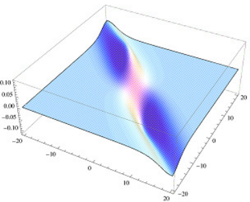
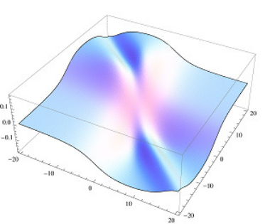
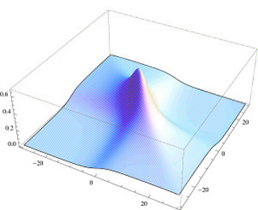
We now list the elementary properties of the modular curvature functions of two variables. (cf. Figures 3, 4, 5)

Lemma 3.1.

The functions $H_{0}(s,t)$ , $H_{1}(s,t)=\cosh\left(\frac{s+t}{2}\right)H_{0}(s,t)$ and $S(s,t)$ fulfill the following properties

(1)

They belong to $C^{\infty}_{0}({\mathbb{R}}^{2})$ .
(2)

$H_{j}(t,s)=-H_{j}(s,t)$ , $S(t,s)=S(s,t)$ and $S(s,t)\geq 0$ .
(3)

$H_{j}(-s,-t)=-H_{j}(s,t)$ , $S(-s,-t)=S(s,t)$ .

Proof.

The smoothness of $H_{0}$ is clear outside the three lines $L_{1}:s+t=0$ , $L_{2}:s=0$ and $L_{3}:t=0$ . Let $n(s,t)$ be the numerator of the fraction defining $H_{0}$ . Near the first line one gets the expansion

n(s,t)=\frac{1}{6}(-2s-s\cosh(s)+3\sinh(s))(s+t)^{3}+\frac{1}{12}(2-2\cosh(s)+s\sinh(s))(s+t)^{4}

+\frac{1}{120}(-2s-3s\cosh(s)+5\sinh(s))(s+t)^{5}+O(s+t)^{6}

which shows that as long as $(s,t)\neq(0,0)$ the function $H_{0}$ is smooth at $(s,t)\in L_{1}$ . The value of $H_{0}$ on $L_{1}$ is given by

H_{0}(s,-s)=-\frac{4\left(3-3e^{2s}+s+4e^{s}s+e^{2s}s\right)}{3\left(\left(-1+e^{s}\right)^{2}s^{2}\right)}

(73)

Refer to caption — Figure 3. Graph of the function $H_{0}$ .

Near the second line $L_{2}$ one gets the expansion

n(s,t)=\frac{1}{2}\left(4+t^{2}-4\cosh(t)+t\sinh(t)\right)s^{2}+\frac{1}{6}(2t+t\cosh(t)-3\sinh(t))s^{3}+O(s)^{4}

which gives the smoothness for $(s,t)$ on the second line (and the third similarly). One needs to look carefully at what happens at the crossing point $(s,t)=(0,0)$ . One finds that the Taylor expansion of $H_{0}$ at the point $(0,0)$ is of the form

H_{0}(s,t)=-\frac{s}{45}+\frac{t}{45}+\frac{s^{3}}{504}+\frac{s^{2}t}{840}-\frac{st^{2}}{840}-\frac{t^{3}}{504}-\frac{s^{3}t^{2}}{6720}+\frac{s^{2}t^{3}}{6720}

-\frac{47s^{4}t}{201600}+\frac{47st^{4}}{201600}-\frac{67s^{5}}{604800}+\frac{67t^{5}}{604800}+\ldots

Similarly we let $m(s,t)$ be the numerator of the fraction defining $S(s,t)$

m(s,t)=(s+t-t\,\cosh(s)-s\,\cosh(t)-\sinh(s)-\sinh(t)+\sinh(s+t))

and get the expansion near the line $L_{1}$ in the form

m(s,t)=(2-2\cosh(s)+s\sinh(s))(s+t)+\frac{1}{2}(-s\cosh(s)+\sinh(s))(s+t)^{2}

+\frac{1}{6}(1-\cosh(s)+s\sinh(s))(s+t)^{3}+O(s+t)^{4}

Near the second line $L_{2}$ one gets the expansion

m(s,t)=\frac{1}{2}(-t+\sinh(t))s^{2}+\frac{1}{6}(-1+\cosh(t))s^{3}+O[s]^{4}

The denominator of $S$ is

s\,t\,\sinh\left(\frac{s}{2}\right)\sinh\left(\frac{t}{2}\right)\sinh\left(\frac{s+t}{2}\right)

and this gives the smoothness outside the origin. At $(0,0)$ one has the Taylor expansion

S(s,t)=\frac{2}{3}-\frac{s^{2}}{45}-\frac{st}{30}-\frac{t^{2}}{45}+\frac{s^{4}}{1260}+\frac{s^{3}t}{504}+\frac{s^{2}t^{2}}{378}+\frac{st^{3}}{504}+\frac{t^{4}}{1260}+\ldots

We now look at the behavior at $\infty$ . It is enough to show that the function $H_{1}(s,t)=\cosh\left(\frac{s+t}{2}\right)H_{0}(s,t)$ tends to $0$ at $\infty$ . We write $H_{1}(s,t)$ as the fraction

\frac{t(s+t)\cosh(s)-s(s+t)\cosh(t)+(s-t)(s+t+\sinh(s)+\sinh(t)-\sinh(s+t))}{st(s+t)\sinh\left(\frac{s}{2}\right)\sinh\left(\frac{t}{2}\right){\rm tanh}\left(\frac{s+t}{2}\right)\sinh\left(\frac{s+t}{2}\right)}

(74)

First note the equality

\sup\{|s|,|t|,|s+t|\}=\frac{1}{2}\left(|s|+|t|+|s+t|\right)\,,\quad~\forall s,t\in{\mathbb{R}}.

(75)

which shows that away from the lines $L_{j}$ the numerator and denominator have the same exponential increase. Let $||(s,t)||_{1}=|s|+|t|$ . The maximum of $|H_{1}(s,t)|$ on the sphere $S_{a}=\{(s,t)\mid||(s,t)||_{1}=a\}$ is reached on the interval

I_{a}=\{(s,-a+s)\mid s\in[\frac{a}{2},a]\}

Away from the boundary of this interval one can approximate the denominator of $H_{1}$ by the product of the leading exponentials which gives

\frac{1}{8}e^{\frac{s}{2}-\frac{t}{2}+\frac{s+t}{2}}st(s+t)

Using this approximation and neglecting terms which are suppressed by an exponential one reduces the function $H_{1}(s,t)$ well inside the interval $I_{a}$ to the fraction

r(s,t)=-\frac{4((-1+t)t+s(1+t))}{st(s+t)}

On $I_{a}$ the function $r(s,t)$ reaches its minimum at $(s,t)=(\frac{a}{2}+v\sqrt{a},-\frac{a}{2}+v\sqrt{a})$ where $v\sim\frac{1}{\sqrt{2}}$ fulfills

1-2v^{2}-\frac{12v^{2}}{a}+\frac{8v^{3}}{\sqrt{a}}-\frac{8v^{4}}{a}=0

One finds in this way that the maximum of $|H_{1}(s,t)|$ on the sphere $S_{a}=\{(s,t)\mid||(s,t)||_{1}=a\}$ is of the order of $\frac{8}{a}$ . One needs to control the size of the function $H_{1}(s,t)$ in the neighborhood of the zeros of the denominator. The restriction of $H_{1}(s,t)$ to the anti-diagonal $t=-s$ is given by the odd function

H_{1}(s,-s)=(-\frac{4s}{3}-\frac{2}{3}s\cosh(s)+2\sinh(s))/s^{2}\sinh(s/2)^{2}

which is equivalent to $-\frac{4}{3}\frac{1}{s}$ when $s\to\pm\infty$ . The restriction of $H_{1}(s,t)$ to the axis $t=0$ is given by

H_{1}(s,0)=-\frac{(4+s^{2}-4\,\cosh(s)+s\,\sinh(s))\cosh(s/2)}{s^{2}\sinh(s/2)^{3}}

which is equivalent to $-\frac{2}{s}$ when $s\to\pm\infty$ .

The restriction of $S(s,t)$ to the anti-diagonal $t=-s$ is given by

\frac{4\left(-2+s\,\text{cotanh}(\frac{s}{2})\right)}{s^{2}}

which behaves like $\frac{4}{s}$ for $s\to\pm\infty$ and this gives the behavior of the maximum of $|S(s,t)|$ on the sphere $S_{a}=\{(s,t)\mid||(s,t)||_{1}=a\}$ . The minimum of $S(s,t)$ on the sphere $S_{a}$ is reached on the diagonal $s=t$ where the function reduces to

S(x,x)=\frac{4}{x^{2}}-\frac{4}{x\sinh(x)}\geq 0

The other properties can be checked in a straightforward manner. ∎

3.2. Local curvature functionals

With the above notation, we are now ready to express in local terms the value at the origin of the zeta functions of the modular spectral triple of weight $\varphi$

(A_{\theta}^{\infty},{\mathcal{H}},{\bar{D}_{\varphi}}).

For each $a\in A_{\theta}^{\infty}$ we consider the zeta function

\displaystyle\zeta_{\triangle_{\varphi}}(a,z)={\rm Tr}(a\,\triangle_{\varphi}^{-z}\,(1-P_{\varphi})),\quad\Re z>2,

(76)

where $P_{\varphi}$ stands for the orthogonal projection onto ${\rm Ker}\triangle_{\varphi}$ . It is related to the theta function by the Mellin transform

\displaystyle\zeta_{\triangle_{\varphi}}(a,z)\,=\,\frac{1}{\Gamma(z)}\int_{0}^{\infty}t^{z-1}\,\left({\rm Tr}(a\,e^{-t\triangle_{\varphi}})-{\rm Tr}(P_{\varphi}\,a\,P_{\varphi})\right)\,dt\,.

(77)

As in the untwisted case, cf. (61), its value at $0$ is related to the constant term in the asymptotic expansion (58), via

\displaystyle\zeta_{\triangle_{\varphi}}(a,0)\,=\,{\rm a}_{2}(a,\triangle_{\varphi})\,-\,{\rm Tr}(P_{\varphi}\,a\,P_{\varphi}).

(78)

The computation of the constant term ${\rm a}_{2}(a,\triangle_{\varphi})$ is quite formidable, as could be expected from the already laborious calculations performed in [7] and [14] in the untwisted case, i.e. $a=1$ . For the clarity of the exposition, we postpone giving the technical details until §6.

On the other hand, the additional term is very easy to compute. Indeed, ${\rm Ker}\triangle_{\varphi}={\rm Ker}(\delta k)$ is one dimensional and one has (with $\varphi_{n}$ the associated state)

{\rm Tr}(P_{\varphi}\,a\,P_{\varphi})=\varphi_{0}(ak^{-2})/\varphi_{0}(k^{-2})=\frac{\varphi(a)}{\varphi(1)}=\varphi_{n}(a)\,.

(79)

One deals in a similar manner with the Laplacian $\triangle^{(0,1)}_{\varphi}$ and one lets $P^{(0,1)}$ be the orthogonal projection on its one-dimensional kernel, ${\rm Ker}\triangle^{(0,1)}_{\varphi}={\rm Ker}(k\delta^{*})$ which is independent of $k$ , and consists of the constant multiples of the unit $1\in A_{\theta}$ , so that

{\rm Tr}(P^{(0,1)}\,a\,P^{(0,1)})=\varphi_{0}(a).

(80)

Theorem 3.2.

Let $\varphi$ be a conformal weight with dilaton $h=h^{\ast}\in A_{\theta}^{\infty}$ and let $k=e^{h/2}$ . The value at the origin of the zeta function associated to the modular spectral triple of weight $\varphi$ is given for any $a\in A_{\theta}^{\infty}$ by the expression

	$\displaystyle{\rm Tr}(a\|{\bar{D}_{\varphi}}\|^{-z})\big\|_{z=0}$	$\displaystyle=$	$\displaystyle-\frac{\pi}{\tau_{2}}\varphi_{0}(a\left(K(\nabla)(\triangle(\log k))+H(\nabla_{1},\nabla_{2})(\square_{\Re}(\log k)\right.)$		(81)
		$\displaystyle+$	$\displaystyle\left.S(\nabla_{1},\nabla_{2})(\square_{\Im}(\log k))\right)-\varphi_{n}(a)\,-\,\varphi_{0}(a)\,,$		(81)

where $H=H_{0}+H_{1}$ and for its graded version by

	$\displaystyle{\rm Tr}(\gamma a\|{\bar{D}_{\varphi}}\|^{-z})\big\|_{z=0}$	$\displaystyle=$	$\displaystyle-\frac{\pi}{\tau_{2}}\varphi_{0}(a\left(K_{\gamma}(\nabla)(\triangle(\log k))+H_{\gamma}(\nabla_{1},\nabla_{2})(\square_{\Re}(\log k)\right.)$		(82)
		$\displaystyle-$	$\displaystyle\left.S(\nabla_{1},\nabla_{2})(\square_{\Im}(\log k))\right)-\varphi_{n}(a)\,+\,\varphi_{0}(a).$		(82)

where $H_{\gamma}=H_{0}-H_{1}$ .

In order to check the normalization constants we compare this result with the classical formula for the value at $0$ of the zeta function of the Laplacian on a closed surface $\Sigma$

\zeta(0)+{\rm Card}\{j\mid\lambda_{j}=0\}=\frac{1}{12\pi}\int_{\Sigma}\,R\sqrt{g}d^{2}x=\frac{1}{6}\,\chi(\Sigma)\,,

(83)

where $R$ is the scalar curvature (normalized as being $1$ for the unit two sphere) and $\chi(\Sigma)$ the Euler-Poincaré characteristic. One double checks this formula for the unit two sphere, whose Laplacian spectrum is the set $\{n^{2}+n\mid n\in{\mathbb{Z}}_{+}\}$ where the eigenvalue $n^{2}+n$ has multiplicity $2n+1$ . One has

\sum_{{\mathbb{Z}}_{+}}(2n+1)e^{-t(n^{2}+n)}\sim\frac{1}{t}+\frac{1}{3}+O(t)

whose constant term $\frac{1}{3}$ agrees with the right hand side $\frac{1}{6}\,\chi(S^{2})$ of (83). In a local form one has

{\rm Tr}(a\Delta^{-z})\big|_{z=0}+{\rm Tr}(aP)=\frac{1}{12\pi}\int_{\Sigma}a\,R\sqrt{g}d^{2}x

(84)

where $P$ is the orthogonal projection on the kernel of the Laplacian. To compare this formula with Theorem 3.2 we take the half sum of (81) and (82) in the commutative case. This reduces to

{\rm Tr}(a\Delta^{-z})\big|_{z=0}+{\rm Tr}(aP)=-\frac{\pi}{\tau_{2}}\varphi_{0}(aK_{0}(0)\triangle(\log k))

(85)

One has $K_{0}(0)=\frac{1}{3}$ and $\varphi_{0}$ is the state associated to the volume form of the flat two torus with integral spectrum. To check the overall normalization we take $\tau=i$ so that $\tau_{2}=1$ . The torus has coordinates $x_{j}$ with period $2\pi$ , Riemannian metric $ds^{2}=dx_{1}^{2}+dx_{2}^{2}$ , and the spectrum of the Laplacian is the set $\{n^{2}+m^{2}\mid n,m\in{\mathbb{Z}}\}$ . Thus

\varphi_{0}(a)=\frac{1}{(2\pi)^{2}}\int adx_{1}dx_{2}\,,\ \ \triangle(f)=-(\partial_{1}^{2}+\partial_{2}^{2})f\,.

(86)

We now consider the Riemannian metric $g=k^{-2}(dx_{1}^{2}+dx_{2}^{2})$ . Its volume form is $\sqrt{g}d^{2}x=k^{-2}dx_{1}dx_{2}$ . The scalar curvature is

R=k^{2}(\partial_{1}^{2}+\partial_{2}^{2})\log k\,.

(87)

To check this, take the stereographic coordinates on the unit two sphere, so that the metric becomes $g=k^{-2}(dx_{1}^{2}+dx_{2}^{2})$ with $k=\frac{1}{2}(1+x_{1}^{2}+x_{2}^{2})$ . Then (87) gives $R=1$ as required. Thus (84) gives for arbitrary $k$ the local form

{\rm Tr}(a\Delta^{-z})\big|_{z=0}+{\rm Tr}(aP)=\frac{1}{12\pi}\int_{T^{2}}a\,(\partial_{1}^{2}+\partial_{2}^{2})(\log k)d^{2}x

(88)

and this agrees with the right hand side of (85) which is, using (86),

-\frac{\pi}{\tau_{2}}\varphi_{0}(aK_{0}(0)\triangle(\log k))=\pi\frac{1}{3}\varphi_{0}(a\,(\partial_{1}^{2}+\partial_{2}^{2})(\log k))=\frac{1}{12\pi}\int_{T^{2}}a\,(\partial_{1}^{2}+\partial_{2}^{2})(\log k)d^{2}x

The fact that the local curvature expressions, occurring in (81) on the one hand and those occurring in (82) on the other hand, are sharply different stands in stark contrast with the case of the ordinary torus. For the latter they reduce to

\displaystyle-K(0)\,\triangle(\log k)\,k^{2}\,=\,\frac{1}{6}\,\triangle(h)\,e^{h},\quad\text{resp.}\quad-K_{\gamma}(0)\,\triangle(\log k)\,k^{2}\,=\,-\frac{1}{2}\,\triangle(h)\,e^{h},

and thus are both constant multiples of the Gaussian curvature of the conformal metric.

4. Log-determinant functional and scalar curvature

In this section we develop the analogue of the Osgood-Phillips-Sarnak functional [18], which is a scale invariant version of the log-determinant of the Laplacian. We then compute its gradient, whose corresponding flow for Riemann surfaces exactly reproduces Hamilton’s Ricci flow [17], and therefore yields the appropriate analogue of the scalar curvature.

4.1. Variation of the log-determinant

The Ray-Singer zeta function regularization of the determinant of a Laplacian [19], as well as the related notion of analytic torsion [20], make perfect sense in the case of noncommutative $2$ -tori, due to the existence of the appropriate pseudodifferential calculus [8]. Thus,

\displaystyle\log{\rm Det}^{\prime}(\triangle_{\varphi})\,=\,-\zeta^{\prime}_{\triangle_{\varphi}}(0),\quad\text{resp.}\quad\log{\rm Det}^{\prime}(\triangle^{(0,1)}_{\varphi})\,=\,-\zeta^{\prime}_{\triangle^{(0,1)}_{\varphi}}(0),

are well-defined. Because $\triangle_{\varphi}=k\delta\delta^{*}k$ and $\triangle^{(0,1)}_{\varphi}=\delta^{*}k^{2}\delta$ have the same spectrum outside $0$ , and so the corresponding zeta functions coincide, the two log-determinants are in fact equal.

In order to compute the above determinant, let us consider again the $1$ -parameter family of Laplacians, cf. (65),

\triangle_{sh}:=\,k^{s}\,\triangle\,k^{s}\,=\,e^{\frac{sh}{2}}\,\triangle\,e^{\frac{sh}{2}},\qquad s\in{\mathbb{R}}.

Differentiating the corresponding family of zeta functions and taking into account (66) one obtains, for $\Re z>p\,$ ,

\displaystyle\begin{split}&\frac{d}{ds}\zeta_{\triangle_{sh}}(z)\,=\,\frac{1}{\Gamma(z)}\int_{0}^{\infty}t^{z}\,\frac{d}{dt}{\rm Tr}\left(he^{-t\triangle_{sh}}(1-P_{sh})\right)\,dt\\ &=\frac{1}{\Gamma(z)}\,t^{z}\,{\rm Tr}\left(he^{-t\triangle_{sh}}(1-P_{sh})\right)\bigg|_{0}^{\infty}\,-\,\frac{z}{\Gamma(z)}\int_{0}^{\infty}t^{z-1}\,{\rm Tr}\left(he^{-t\triangle_{sh}}(1-P_{sh})\right)\,dt\\ &=\,-\frac{z}{\Gamma(z)}\int_{0}^{\infty}t^{z-1}\,{\rm Tr}\left(he^{-t\triangle_{sh}}(1-P_{sh})\right)\,dt\,=:\,-z\,\zeta_{\triangle_{sh}}(h,z).\end{split}

By meromorphic continuation one obtains the identity

\displaystyle\frac{d}{ds}\zeta_{\triangle_{sh}}(z)\,=\,-z\,\zeta_{\triangle_{sh}}(h,z),\quad\forall\,z\in\mathbb{C},

(89)

and taking $\displaystyle\frac{d}{dz}\bigg|_{z=0}$ yields the variation formula

\displaystyle-\frac{d}{ds}\zeta^{\prime}_{\triangle_{sh}}(0)\,=\,\zeta_{\triangle_{sh}}(h,0).

(90)

Applying Theorem 3.2 to the conformal weights $\varphi_{s}$ with dilaton $sh$ , and retaining only the even part of the expression in the right hand side, yields

\displaystyle\begin{split}-\frac{d}{ds}\zeta^{\prime}_{\triangle_{sh}}(0)\,=-\frac{\pi}{\tau_{2}}\,&\,\varphi_{0}\left(h\big(sK_{0}(s\nabla)(\triangle(\frac{h}{2}))+s^{2}H_{0}(s\nabla_{1},s\nabla_{2})(\square_{\Re}(\frac{h}{2}))\big)\right)\\ &-\,\varphi_{n}(h),\end{split}

(91)

One has $\varphi_{n}(h)=-\frac{d}{ds}\log\varphi_{0}(e^{-sh})$ and so by integration along the interval $0\leq s\leq 1$ one obtains the following conformal variation formula.

Lemma 4.1.

Let $\varphi$ be a conformal weight with dilaton $h=h^{\ast}\in A_{\theta}^{\infty}$ . Then

	$\displaystyle\log{\rm Det}^{\prime}(\triangle_{\varphi})$	$\displaystyle=\,\log{\rm Det}^{\prime}\triangle\,+\,\log\varphi(1)$		(92)
		$\displaystyle-\frac{\pi}{\tau_{2}}\int_{0}^{1}\varphi_{0}\left(h\big(sK_{0}(s\nabla)(\triangle(\log k))+s^{2}H_{0}(s\nabla_{1},s\nabla_{2})(\square_{\Re}(\log k))\big)\right)ds$

We now show that this formula simplifies much further.

Lemma 4.2.

For $f(u)$ a function in Schwartz space one has

\varphi_{0}(hf(\nabla)(a))=f(0)\varphi_{0}(ha)\,,\quad~\forall a\in A_{\theta}^{\infty}.

(93)

Proof.

The derivation $\nabla$ is given by the commutator with $-h$ and $\sigma_{t}=\Delta^{-it}$ fixes $h$ and preserves the trace $\varphi_{0}$ . Thus writing $f$ as a Fourier transform

\varphi_{0}(hf(\nabla)(a))=\int g(t)\varphi_{0}(h\sigma_{t}(a))dt=\int g(t)\varphi_{0}(\sigma_{t}(ha))dt=f(0)\varphi_{0}(ha).

∎

We thus get that

\varphi_{0}\left(h\big(sK_{0}(s\nabla)(\triangle(\frac{h}{2})\right)=\frac{1}{2}K_{0}(0)s\varphi_{0}(h\triangle h)=\frac{s}{6}\varphi_{0}(h\triangle h)

and integrating from $0$ to $1$ we obtain, under the hypothesis of Lemma 4.1,

	$\displaystyle\log{\rm Det}^{\prime}(\triangle_{\varphi})$	$\displaystyle=\,\log{\rm Det}^{\prime}\triangle\,+\,\log\varphi(1)-\frac{\pi}{12\tau_{2}}\varphi_{0}(h\triangle h)$		(94)
		$\displaystyle-\frac{\pi}{\tau_{2}}\int_{0}^{1}\varphi_{0}\left(hs^{2}H_{0}(s\nabla_{1},s\nabla_{2})(\square_{\Re}(\log k))\right)ds$

Let us now simplify the last term of (94). By construction the expression $S=\square_{\Re}(\log k)$ can be expressed as a linear combination of squares of elements of $A_{\theta}^{\infty}$ . Thus we really need to understand the quadratic form

Q(x)=\int_{0}^{1}\varphi_{0}\left(hH_{0}(s\nabla_{1},s\nabla_{2})(xx)\right)s^{2}ds

(95)

where writing $H_{0}$ as a Fourier transform

H_{0}(u,v)=\int g(a,b)e^{-i(au+bv)}dadb

(96)

one has

H_{0}(s\nabla_{1},s\nabla_{2})(xx)=\int g(a,b)\sigma_{sa}(x)\sigma_{sb}(x)dadb.

Lemma 4.3.

Let $k(u,v)$ be a Schwartz function, such that $k(v,u)=-k(u,v)$ , then

\varphi_{0}(hk(\nabla_{1},\nabla_{2})(xx))=-\frac{1}{2}\varphi_{0}(\ell(\nabla)(x)x)

(97)

where the function $\ell$ is given by

\ell(u)=u\,k(u,-u)

(98)

Proof.

Let us define the function of two variables

w(a,b)=\varphi_{0}(h\sigma_{a}(x)\sigma_{b}(x))

(99)

so that, with $k(u,v)=\int g(a,b)e^{-i(au+bv)}dadb$ one has

\varphi_{0}(hk(\nabla_{1},\nabla_{2})(xx))=\int g(a,b)w(a,b)dadb

(100)

One has, using $\sigma_{c}(h)=h$ for all $c$ ,

•

$w(a+c,b+c)=w(a,b)$ for all $c$ .
•

$w(a,b)-w(b,a)=-\varphi_{0}(\nabla(\sigma_{a}(x))\sigma_{b}(x))$

where the last equality follows, using the trace property of $\varphi_{0}$ , from

\varphi_{0}(h\sigma_{a}(x)\sigma_{b}(x)-h\sigma_{b}(x)\sigma_{a}(x))=\varphi_{0}([h,\sigma_{a}(x)]\sigma_{b}(x))\,.

Thus one gets, using the antisymmetry of $k(u,v)$ and $g(a,b)$ ,

\varphi_{0}(hk(\nabla_{1},\nabla_{2})(xx))=-\frac{1}{2}\int g(a,b)\varphi_{0}(\nabla(\sigma_{a-b}(x))x)dadb

Moreover

k(u,-u)=\int g(a,b)e^{-i(au-bu)}dadb

and one gets

\varphi_{0}(hk(\nabla_{1},\nabla_{2})(xx))=-\frac{1}{2}\varphi_{0}(\nabla(k(\nabla,-\nabla)(x))x)

which is the required equality. ∎

We used the hypothesis that $k$ is a Schwartz function in order to use freely the Fourier transform but since the spectrum of the operator $\nabla$ is bounded this hypothesis is not needed as long as we deal with smooth functions. It follows using $k(u,v)=H_{0}(su,sv)$ that

\varphi_{0}(hH_{0}(s\nabla_{1},s\nabla_{2})(xx))=\frac{1}{s}\varphi_{0}(L_{0}(s\nabla)(x)x)

(101)

where the function $L_{0}$ is given by

L_{0}(u)=-\frac{1}{2}uH_{0}(u,-u)

(102)

We now need to compute the integral in the variable $s$ of (95).

Lemma 4.4.

Q(x)=\varphi_{0}(K_{2}(\nabla)(x)x)

(103)

where the function $K_{2}$ is given by

K_{2}(v)=\frac{1}{3}+\frac{4}{v^{2}}-\frac{2{\rm coth}(\frac{v}{2})}{v}

(104)

Proof.

One has, by (73),

L_{0}(u)=\frac{2}{3}-\frac{2{\rm coth}\left(\frac{u}{2}\right)}{u}+\sinh\left(\frac{u}{2}\right)^{-2}

Thus, using (101),

Q(x)=\int_{0}^{1}\varphi_{0}\left(hH_{0}(s\nabla_{1},s\nabla_{2})(xx)\right)s^{2}ds=\int_{0}^{1}\varphi_{0}(L_{0}(s\nabla)(x)x)sds

which gives (103) for

K_{2}(v)=\int_{0}^{1}L_{0}(sv)sds=v^{-2}\int_{0}^{v}uL_{0}(u)du,

and one checks that this agrees with (104) by showing that the derivative of $v^{2}K_{2}(v)$ is $vL_{0}(v)$ . ∎

We can thus simplify (94) and obtain, using $\log k=\frac{h}{2}$ ,

\log{\rm Det}^{\prime}(\triangle_{\varphi})=\,\log{\rm Det}^{\prime}\triangle\,+\,\log\varphi(1)-\frac{\pi}{12\tau_{2}}\varphi_{0}(h\triangle h)-\frac{\pi}{4\tau_{2}}\varphi_{0}\left(K_{2}(\nabla_{1})(\square_{\Re}(h))\right)

(105)

Remark 4.5.

Since $\triangle$ is isospectral to the Dolbeault-Laplacian on ${\rm T}^{2}$ whose spectrum is the set of $|n+m\tau|^{2}$ for $n,m\in{\mathbb{Z}}$ , $(n,m)\neq(0,0)$ , $\,\log{\rm Det}^{\prime}\triangle$ remains the same as for the ordinary $2$ -torus, and is computed by the Kronecker limit formula, as in [20, Theorem 4.1]; explicitly,

\displaystyle\log{\rm Det}^{\prime}\triangle\,=-\frac{d}{ds}\big|_{s=0}\sum_{(n,m)\neq(0,0)}|n+m\tau|^{-2s}=\,\log\left(4\pi^{2}\,|\eta(\tau)|^{4}\right),

where $\eta$ is the Dedekind eta function

\displaystyle\eta(\tau)\,=\,e^{\frac{\pi\,i}{12}\,\tau}\,\prod_{n>0}\left(1-e^{2\pi in\tau}\right).

Recalling that the logarithm of analytic torsion for a complex curve [20] is given by

\frac{1}{2}\sum_{q=0}^{1}(-1)^{q}\log{\rm Det}^{\prime}(\triangle^{(q,0)})\,=\,-\frac{1}{2}\log{\rm Det}^{\prime}(\triangle^{(1,0)}_{\varphi})\,,

it is perhaps not surprising that the Osgood-Phillips-Sarnak functional [18, §2.1] involves the negative of the log-determinant. By analogy, we define the translation invariant functional $F$ on the space of selfadjoint elements of $A^{\infty}_{\theta}$ by the formula

\displaystyle F(h):=\,-\log{\rm Det}^{\prime}(\triangle_{\varphi})+\log\varphi(1)\,=\,-\log{\rm Det}^{\prime}\left(e^{\frac{h}{2}}\triangle e^{\frac{h}{2}}\right)+\log\varphi_{0}(e^{-h}).

(106)

Its invariance under rescaling is due to the fact that $\zeta_{\triangle_{\varphi}}(0)=-1$ , cf. Theorem 2.2. Indeed, since $\quad\triangle_{h+c}=e^{c}\triangle_{h}$ for any $\,c\in{\mathbb{R}}$ , one has

\displaystyle\zeta_{\triangle_{h+c}}(z)\,=\,e^{-cz}\,\zeta_{\triangle_{h}}(z),

it follows that

\displaystyle\begin{split}F(h+c)&=\,\zeta^{\prime}_{\triangle_{h+c}}(0)\,+\,\log\varphi_{0}(e^{-h-c})\,=\,-c\,\zeta_{\triangle_{h}}(0)\,+\,\zeta^{\prime}_{\triangle_{h}}(0)\,\\ &\,+\log\varphi_{0}(e^{-c})\,+\,\log\varphi_{0}(e^{-h})\,=\,F(h).\end{split}

Theorem 4.6.

The functional $F(h)$ has the expression

F(h)=\,-\log\left(4\pi^{2}\,|\eta(\tau)|^{4}\right)+\frac{\pi}{4\tau_{2}}\varphi_{0}\left((K_{2}-\frac{1}{3})(\nabla_{1})(\square_{\Re}(h))\right).

(107)

One has $F(h)\geq F(0)$ for all $h$ and equality holds if and only if $h$ is a scalar.

Proof.

One obtains using (105) and the classical value for $h=0$

	$\displaystyle F(h)$	$\displaystyle=$	$\displaystyle\,-\log\left(4\pi^{2}\,\|\eta(\tau)\|^{4}\right)+\frac{\pi}{12\tau_{2}}\varphi_{0}(h\triangle h)$		(108)
		$\displaystyle+$	$\displaystyle\frac{\pi}{4\tau_{2}}\varphi_{0}\left(K_{2}(\nabla_{1})(\square_{\Re}(h))\right).$		(108)

Using integration-by-parts with respect to the derivation $\delta^{\ast}$ , one sees that

\displaystyle\varphi_{0}\big(h\,\triangle(h)\big)\,=\,\varphi_{0}\big(h\,\delta^{\ast}(\delta(h))\big)\,=\,-\varphi_{0}\big(\delta^{\ast}(h)\,\delta(h)\big)\,=\,\varphi_{0}\big(\delta(h)^{\ast}\,\delta(h)\big).

(109)

Note that the skew term

\varphi_{0}(-i\tau_{2}\delta_{2}(h)^{*}\delta_{1}(h)+i\tau_{2}\delta_{1}(h)^{*}\delta_{2}(h))=-i\tau_{2}\varphi_{0}([\delta_{1}(h),\delta_{2}(h)])=0

vanishes. Thus one has

\varphi_{0}\big(h\,\triangle(h)\big)=-\varphi_{0}(\square_{\Re}(h)).

(110)

This, together with (108) gives (107).

Figure 6. Graph of the function

\frac{1}{3}-K_{2}

, even and positive.

In the Hilbert space ${\mathcal{H}}_{0}$ with inner product (19), the operator $\nabla$ which is given by $a\mapsto-[h,a]$ is bounded and self-adjoint since

\langle\nabla(a),b\rangle=-\varphi_{0}(b^{*}[h,a])=\varphi_{0}((-[h,b])^{*}a)=\langle a,\nabla(b)\rangle

Since the function $\frac{1}{3}-K_{2}$ is even and strictly positive, it follows that the equality

\langle a,b\rangle_{k}=\langle(\frac{1}{3}-K_{2})(\nabla)(a),b\rangle

(111)

defines a non degenerate positive symmetric inner product on ${\mathcal{H}}_{0}$ . Now by (107), and the skew adjointness $\delta_{j}(h)^{*}=-\delta_{j}(h)$ one has

\varphi_{0}\left((K_{2}-\frac{1}{3})(\nabla_{1})(\square_{\Re}(h))\right)=\langle\delta_{1}(h),\delta_{1}(h)\rangle_{k}+2\Re(\tau)\langle\delta_{1}(h),\delta_{2}(h)\rangle_{k}+|\tau|^{2}\langle\delta_{2}(h),\delta_{2}(h)\rangle_{k}

and thus

F(h)=F(0)+\frac{\pi}{4\tau_{2}}\langle\delta(h),\delta(h)\rangle_{k}

(112)

This shows that $F(h)\geq F(0)$ and moreover the equality holds only if $\delta(h)=0$ which implies that $h$ is a constant. ∎

Remark 4.7.

Note that the first term in the right hand side of (108) matches the expression of the functional in the commutative case (cf. [18, §3]), while the second term is of a purely modular nature and is highly non-linear.

4.2. Gradient flow and scalar curvature

Identifying the tangent space to the dilatons with the selfadjoint elements of $A_{\theta}^{\infty}$ , and using the inner product given by $\varphi_{0}$ , we shall define the gradient of the functional $F$ by means of the Gâteaux differential:

\displaystyle\varphi_{0}(a\,{\rm grad}_{h}F)\,=\,\langle{\rm grad}_{h}F,a\rangle\,=\,\frac{d}{d\varepsilon}\big|_{\varepsilon=0}F(h+\varepsilon a),\qquad\forall\,a=a^{\ast}\in A_{\theta}^{\infty},

(113)

Theorem 4.8.

The gradient of $F$ is given by the expression

{\rm grad}_{h}F=\frac{\pi}{4\tau_{2}}\left(\tilde{K}_{0}(\nabla)(\triangle(h))+\frac{1}{2}\tilde{H}_{0}(\nabla_{1},\nabla_{2})(\square_{\Re}(h))\right)

(114)

where the functions $\tilde{K}_{0}$ and $\tilde{H}_{0}$ are directly related to $K_{0}$ , $K_{2}$ and $H_{0}$ by

\tilde{K}_{0}(s)=4\frac{\sinh(s/2)}{s}K_{0}(s)=-2\left(K_{2}(s)-\frac{1}{3}\right)

(115)

and

\tilde{H}_{0}(s,t))=4\frac{\sinh((s+t)/2)}{s+t}H_{0}(s,t).

(116)

Proof.

Consider the $1$ -parameter family of operators

{\tilde{\triangle}_{\varepsilon}}\,=\,e^{\frac{h+\varepsilon a}{2}}\,\triangle\,e^{\frac{h+\varepsilon a}{2}},\qquad\varepsilon>0.

The Duhamel (also the expansional) formula implies that

\displaystyle\frac{d}{d\varepsilon}\big|_{\varepsilon=0}e^{\frac{h+\varepsilon a}{2}}\,=\,\frac{1}{2}\,\int_{0}^{1}e^{\frac{uh}{2}}\,a\,e^{\frac{(1-u)h}{2}}\,du,

hence

\displaystyle\begin{split}\frac{d}{d\varepsilon}\big|_{\varepsilon=0}{\tilde{\triangle}_{\varepsilon}}\,=\,\frac{1}{2}\int_{0}^{1}e^{\frac{uh}{2}}\,a\,e^{-\frac{uh}{2}}\,du\,\triangle_{h}\,+\,\frac{1}{2}\triangle_{h}\,\int_{0}^{1}e^{-\frac{(1-u)h}{2}}\,a\,e^{\frac{(1-u)h}{2}}\,du.\end{split}

It follows that

\displaystyle\begin{split}&\frac{d}{d\varepsilon}\big|_{\varepsilon=0}{\rm Tr}\left(e^{-t{\tilde{\triangle}_{\varepsilon}}}\right)\,=\,-t\,{\rm Tr}\left(\frac{d}{d\varepsilon}\big|_{\varepsilon=0}({\tilde{\triangle}_{\varepsilon}})\,e^{-t\triangle_{h}}\right)\,=\\ &=\,-\frac{t}{2}\,{\rm Tr}\left(\int_{0}^{1}e^{\frac{uh}{2}}\,a\,e^{-\frac{uh}{2}}\,du\,\triangle_{h}\,e^{-t\triangle_{h}}\right)\,\,-\frac{t}{2}\,{\rm Tr}\left(\triangle_{h}\,\int_{0}^{1}e^{-\frac{(1-u)h}{2}}\,a\,e^{\frac{(1-u)h}{2}}\,du\,e^{-t\triangle_{h}}\right)\\ &=\,-\frac{t}{2}\,{\rm Tr}\left(\triangle_{h}\,e^{-t\triangle_{h}}\,\int_{0}^{1}e^{\frac{uh}{2}}\,a\,e^{-\frac{uh}{2}}\,du\right)\,-\,\frac{t}{2}\,{\rm Tr}\left(e^{-t\triangle_{h}}\,\triangle_{h}\,\int_{0}^{1}e^{-\frac{uh}{2}}\,a\,e^{\frac{uh}{2}}\,du\right)\\ &=\,-\frac{t}{2}\,{\rm Tr}\left(\triangle_{h}\,e^{-t\triangle_{h}}\,\int_{-1}^{1}e^{\frac{uh}{2}}\,a\,e^{-\frac{uh}{2}}\,du\right)\,=\,\frac{t}{2}\,\frac{d}{dt}\,{\rm Tr}\left(e^{-t\triangle_{h}}\,\int_{-1}^{1}e^{\frac{uh}{2}}\,a\,e^{-\frac{uh}{2}}\,du\right).\end{split}

(117)

Differentiating at $\varepsilon=0$ the $1$ -parameter family of the zeta functions

\displaystyle\zeta_{{\tilde{\triangle}_{\varepsilon}}}(z)={\rm Tr}\left((1-P_{\varepsilon}){\tilde{\triangle}_{\varepsilon}}^{-z}\right),\quad\Re z>p,

and taking into account the above identity, one obtains for $\Re z>p\,$ ,

\displaystyle\begin{split}\frac{d}{d\varepsilon}\big|_{\varepsilon=0}\zeta_{{\tilde{\triangle}_{\varepsilon}}}(z)&=\,\frac{1}{\Gamma(z)}\int_{0}^{\infty}t^{z-1}\,\frac{d}{d\varepsilon}\big|_{\varepsilon=0}{\rm Tr}\left(e^{-t{\tilde{\triangle}_{\varepsilon}}}(1-P_{\varepsilon})\right)\,dt\\ &=\,\frac{1}{\Gamma(z)}\int_{0}^{\infty}t^{z-1}\,\frac{d}{d\varepsilon}\big|_{\varepsilon=0}{\rm Tr}\left(e^{-t{\tilde{\triangle}_{\varepsilon}}}\right)\,dt\\ &=\,\frac{1}{2\,\Gamma(z)}\int_{0}^{\infty}t^{z}\,\frac{d}{dt}\,{\rm Tr}\left(e^{-t\triangle_{h}}\,\int_{-1}^{1}e^{\frac{uh}{2}}\,a\,e^{-\frac{uh}{2}}\,du\right)\,dt\\ &=\frac{1}{2\,\Gamma(z)}\,t^{z}\,{\rm Tr}\left(e^{-t\triangle_{h}}(1-P_{h})\,\int_{-1}^{1}e^{\frac{uh}{2}}\,a\,e^{-\frac{uh}{2}}\,du\right)\bigg|_{0}^{\infty}\\ &-\,\frac{z}{2\,\Gamma(z)}\int_{0}^{\infty}t^{z-1}\,{\rm Tr}\left(he^{-t\triangle_{h}}(1-P_{h})\int_{-1}^{1}e^{\frac{uh}{2}}\,a\,e^{-\frac{uh}{2}}\,du\right)\,dt\\ &=\,-\frac{z}{2\,\Gamma(z)}\int_{0}^{\infty}t^{z-1}\,{\rm Tr}\left(e^{-t\triangle_{h}}(1-P_{h})\int_{-1}^{1}e^{\frac{uh}{2}}\,a\,e^{-\frac{uh}{2}}\,du\right)\,dt\\ &=\,-\frac{z}{2}\,\zeta_{\triangle_{h}}\left(\int_{-1}^{1}e^{\frac{uh}{2}}\,a\,e^{-\frac{uh}{2}}\,du,\,z\right).\end{split}

Now taking the derivative $\displaystyle\frac{d}{dz}\bigg|_{z=0}$ gives

\displaystyle\begin{split}-\,\frac{d}{d\varepsilon}\bigg|_{\varepsilon=0}\zeta^{\prime}_{{\tilde{\triangle}_{\varepsilon}}}(0)&=\,\frac{1}{2}\,\zeta_{\triangle_{h}}\left(\int_{-1}^{1}e^{\frac{uh}{2}}\,a\,e^{-\frac{uh}{2}}\,du,\,0\right)\\ &=\frac{1}{2}\,{\rm a}_{2}\left(\int_{-1}^{1}e^{\frac{uh}{2}}\,a\,e^{-\frac{uh}{2}}\,du,\triangle_{h}\right)-\frac{1}{2}\,{\rm Tr}\left(P_{h}\int_{-1}^{1}e^{\frac{uh}{2}}\,a\,e^{-\frac{uh}{2}}\,du\right)\\ &=\frac{1}{2}\,{\rm a}_{2}\left(\int_{-1}^{1}e^{\frac{uh}{2}}\,a\,e^{-\frac{uh}{2}}\,du,\triangle_{h}\right)-\frac{1}{2}\,\frac{\varphi_{0}\left(\int_{-1}^{1}e^{\frac{uh}{2}}\,a\,e^{-\frac{uh}{2}}\,du\,e^{-h}\right)}{\varphi_{0}(e^{-h})}\\ &=\frac{1}{2}\,{\rm a}_{2}\left(\int_{-1}^{1}e^{\frac{uh}{2}}\,a\,e^{-\frac{uh}{2}}\,du,\triangle_{h}\right)-\,\frac{\varphi_{0}(ae^{-h})}{\varphi_{0}(e^{-h})}.\end{split}

The calculation of the derivative corresponding to the area term is very easy. Indeed, since $\varphi_{0}$ is a trace, one simply has

\displaystyle\frac{d}{d\varepsilon}\big|_{\varepsilon=0}\varphi_{0}(e^{-h-\varepsilon a})\,=\,-\varphi_{0}(ae^{-h}),

hence

\displaystyle\frac{d}{d\varepsilon}\big|_{\varepsilon=0}\log\varphi_{0}(e^{-h-\varepsilon a})=-\frac{\varphi_{0}(ae^{-h})}{\varphi_{0}(e^{-h})}.

Summing up and recalling that by its very definition, cf. (106),

\displaystyle F(h+\varepsilon a):\,=\,-\log{\rm Det}^{\prime}\left(e^{\frac{h+\varepsilon a}{2}}\triangle e^{\frac{h+\varepsilon a}{2}}\right)+\log\varphi_{0}(e^{-h-\varepsilon a}),

one concludes that

\displaystyle\varphi_{0}(a\,{\rm grad}_{h}F)\,=\,-\frac{1}{2}\,\,{\rm a}_{2}\left(\int_{-1}^{1}e^{\frac{uh}{2}}\,a\,e^{-\frac{uh}{2}}\,du,\,\triangle_{h}\right).

(118)

To obtain the claimed expression of the gradient we appeal to Theorem 3.2, move one of the exponential factors under the trace $\varphi_{0}$ , and get

{\rm grad}_{h}F\,=\frac{\pi}{2\tau_{2}}\int_{-1}^{1}e^{\frac{uh}{2}}\left(K_{0}(\nabla)(\triangle(\log k))+H_{0}(\nabla_{1},\nabla_{2})(\square_{\Re}(\log k)\right)e^{-\frac{uh}{2}}\,du

One has

\nabla(x)=-[h,x]\,,\ \ \int_{-1}^{1}e^{\frac{u\nabla}{2}}du=4\frac{\sinh(\nabla/2)}{\nabla}

thus the function $K_{0}$ gets multiplied by $4\sinh(s/2)/s$ and becomes

\tilde{K}_{0}(s)=4\frac{\sinh(s/2)}{s}K_{0}(s)=\frac{4\left(2+e^{s}(-2+s)+s\right)}{\left(-1+e^{s}\right)s^{2}}=4\left(\frac{{\rm coth}(s/2)}{s}-2s^{-2}\right)

similarly, one has

\int_{-1}^{1}e^{\frac{u(\nabla_{1}+\nabla_{2})}{2}}du=4\frac{\sinh((\nabla_{1}+\nabla_{2})/2)}{(\nabla_{1}+\nabla_{2})}

which gives (116). ∎

Remark 4.9.

One may wonder if there is a similar manner of using the local formula for $\triangle^{(0,1)}_{\varphi}$ of Theorem 3.2 to handle $\log{\rm Det}^{\prime}(\triangle^{(0,1)}_{\varphi})=-\zeta^{\prime}_{\triangle^{(0,1)}_{\varphi}}(0)$ . To this end, we start from the equality $\triangle^{(0,1)}_{\varphi}=\delta^{*}k^{2}\delta$ and the $1$ -parameter family

\triangle^{(0,1)}_{\epsilon}:=\,\delta^{*}\,\,e^{h+\varepsilon a}\,\delta,\qquad\epsilon\in{\mathbb{R}}.

Since

\displaystyle\frac{d}{d\varepsilon}\big|_{\varepsilon=0}e^{h+\varepsilon a}\,=\,\int_{0}^{1}e^{uh}\,a\,e^{(1-u)h}\,du,

one has

\displaystyle\begin{split}\frac{d}{d\varepsilon}\big|_{\varepsilon=0}\triangle^{(0,1)}_{\epsilon}\,=\,\int_{0}^{1}\delta^{\star}\,e^{uh}\,a\,e^{(1-u)h}\,\delta\,du.\end{split}

The Duhamel formula

\frac{d}{d\varepsilon}\big|_{\varepsilon=0}e^{-t\triangle^{(0,1)}_{\epsilon}}\,=\,-t\int_{0}^{1}e^{-vt\triangle^{(0,1)}_{\varphi}}\,\frac{d}{d\varepsilon}\big|_{\varepsilon=0}(\triangle^{(0,1)}_{\epsilon})\,e^{-(1-v)t\triangle^{(0,1)}_{\varphi}}\,dv.

implies

\displaystyle\begin{split}&\frac{d}{d\varepsilon}\big|_{\varepsilon=0}{\rm Tr}\left(e^{-t\triangle^{(0,1)}_{\epsilon}}\right)\,=\,-t\,{\rm Tr}\left(\frac{d}{d\varepsilon}\big|_{\varepsilon=0}(\triangle^{(0,1)}_{\epsilon})\,e^{-t\triangle^{(0,1)}_{\varphi}}\right)\,=\\ &=-t\int_{0}^{1}{\rm Tr}\left(\delta^{\star}\,e^{uh}\,a\,e^{(1-u)h}\,\delta\,e^{-t\triangle^{(0,1)}_{\varphi}}\right)\,du\,=\,-t\int_{0}^{1}{\rm Tr}\left(e^{uh}\,a\,e^{(1-u)h}\,\delta\,e^{-t\triangle^{(0,1)}_{\varphi}}\delta^{\star}\right)\,du\\ &=\,-t\int_{0}^{1}{\rm Tr}\left((e^{\frac{(2u-1)h}{2}}\,a\,e^{\frac{(1-2u)h}{2}})\,(e^{\frac{h}{2}}\,\delta\,e^{-t\triangle^{(0,1)}_{\varphi}}\delta^{\star}\,e^{\frac{h}{2}})\right)\,du\\ &=\,-\frac{t}{2}\int_{-1}^{1}{\rm Tr}\left((e^{\frac{vh}{2}}\,a\,e^{-\frac{vh}{2}})\,(e^{\frac{h}{2}}\,\delta\,e^{-t\triangle^{(0,1)}_{\varphi}}\delta^{\star}\,e^{\frac{h}{2}})\right)\,dv.\end{split}

Notice now that

\displaystyle e^{\frac{h}{2}}\,\delta\,e^{-t\triangle^{(0,1)}_{\varphi}}\delta^{\star}\,e^{\frac{h}{2}}\,=\,e^{-t\triangle_{\varphi}}\,\triangle_{\varphi},

reverting us to the expression (117), which involves the local formula for $\triangle_{\varphi}$ and not for $\triangle^{(0,1)}_{\varphi}$ . Thus, one ends up by merely recovering the same expression (114) of the gradient.

Replacing in the definition (113) the fixed inner product by the running one, one could alternatively define the gradient by means of the running inner product, as follows:

\displaystyle\langle{\rm Grad}_{h}F,a\rangle_{\varphi}\,=\,\varphi_{0}(a\,{\rm Grad}_{h}F\,e^{-h})\,=\,\frac{d}{d\varepsilon}\big|_{\varepsilon=0}F(h+\varepsilon a),\qquad\forall\,a=a^{\ast}\in A_{\theta}^{\infty}.

(119)

Then Theorem 4.8 gives

{\rm Grad}_{h}F\,=\,\frac{\pi}{4\tau_{2}}\left(\tilde{K}_{0}(\nabla)(\triangle(h))+\frac{1}{2}\tilde{H}_{0}(\nabla_{1},\nabla_{2})(\square_{\Re}(h))\right)\,e^{h}.

(120)

Based on the analogy with the standard torus (comp. [18, §3, (3.8)]), the right hand side

K_{\varphi}\,=\,\frac{\pi}{4\tau_{2}}\left(\tilde{K}_{0}(\nabla)(\triangle(h))+\frac{1}{2}\tilde{H}_{0}(\nabla_{1},\nabla_{2})(\square_{\Re}(h))\right)\,e^{h}

(121)

can be taken as the appropriate definition of the scalar curvature $K_{\varphi}$ of the conformal metric on the noncommutative torus associated to the given dilaton. The evolution equation for the conformal factor $-h$ becomes

\displaystyle\frac{\partial h}{\partial t}\,=\,K_{\varphi}.

(122)

Unlike the commutative case, the corresponding flow of inner products is not given by the same differential equation. Denoting by $g_{\varphi}$ the Hermitian form

\displaystyle g_{\varphi}(a,b):=\,\langle a,b\rangle_{\varphi}\,=\,\varphi(b^{\ast}a)\,=\,\varphi_{0}(b^{\ast}ae^{-h}),\quad\forall\,a,b\in A_{\theta},

one has

\displaystyle\begin{split}\frac{\partial g_{\varphi}(a,b)}{\partial t}&=\,\varphi_{0}\left(b^{\ast}a\frac{\partial e^{-h}}{\partial t}\right)\,=\,-\varphi_{0}\left(b^{\ast}a\int_{0}^{1}e^{-uh}\frac{\partial h}{\partial t}e^{(u-1)h}\,du\right)\\ &=\,-\varphi_{0}\left(b^{\ast}a\int_{0}^{1}e^{-uh}K_{\varphi}e^{uh}\,du\,e^{-h}\right)\,=\,-\langle a\int_{0}^{1}e^{-uh}K_{\varphi}e^{uh}\,du\,,b\rangle_{\varphi}\,.\end{split}

Denoting by $R_{\varphi}$ the resulting Hermitian form

\displaystyle R_{\varphi}(a,b)\,=\,\langle a\frac{e^{\nabla}-1}{\nabla}(K_{\varphi}),b\rangle_{\varphi}\,,\quad\forall\,a,b\in A_{\theta},

(123)

we conclude that the metric associated to $\varphi$ has evolution equation

\displaystyle\frac{\partial g_{\varphi}}{\partial t}\,=\,-R_{\varphi}.

(124)

Since the average curvature

\varphi(K_{\varphi})\,=\,\varphi_{0}({\rm grad}_{h}F)\,=\,\frac{d}{d\varepsilon}\big|_{\varepsilon=0}F(h+\varepsilon)\,=\,0,

the equation (124) is precisely the analogue of Hamilton’s Ricci flow [17] for the standard torus. This justifies viewing the Hermitian form $R_{\varphi}$ as the Ricci curvature of ${\rm T}^{2}_{\theta}$ endowed with the inner product $g_{\varphi}$ .

4.3. Functional relation between $\tilde{K}_{0}$ and $\tilde{H}_{0}$

We shall now explain how to perform the direct computation of the gradient of an expression of the form

\varphi_{0}\left(G(\nabla_{1})(\square_{\Re}(h))\right)

We shall then show how this, together with Theorem 4.8, implies the following relation between $\tilde{K}_{0}$ and $\tilde{H}_{0}$ ,

-\frac{1}{2}\tilde{H}_{0}(s_{1},s_{2})=\frac{\tilde{K}_{0}(s_{2})-\tilde{K}_{0}(s_{1})}{s_{1}+s_{2}}+\frac{\tilde{K}_{0}(s_{1}+s_{2})-\tilde{K}_{0}(s_{2})}{s_{1}}-\frac{\tilde{K}_{0}(s_{1}+s_{2})-\tilde{K}_{0}(s_{1})}{s_{2}}

(125)

This relation can then be checked directly and gives the following decomposition

-\frac{1}{8}\tilde{H}_{0}(s,t)=\frac{2(s-t)}{st(s+t)^{2}}

+\frac{{\rm coth}\left(\frac{s}{2}\right)}{st}-\frac{{\rm coth}\left(\frac{s}{2}\right)}{s(s+t)}-\frac{{\rm coth}\left(\frac{t}{2}\right)}{st}+\frac{{\rm coth}\left(\frac{t}{2}\right)}{t(s+t)}+\frac{{\rm coth}\left(\frac{s+t}{2}\right)}{s(s+t)}-\frac{{\rm coth}\left(\frac{s+t}{2}\right)}{t(s+t)}\,.

The fact that (125) can be proven on a priori ground gives a handle on the complicated two variable functions which appear in Theorem 3.2 since by (116) one can deduce the function $H_{0}$ from $\tilde{H}_{0}$ . Note moreover that the function $\frac{1}{8}\tilde{K}_{0}$ is the generating function for Bernoulli numbers since one has

\frac{1}{8}\tilde{K}_{0}(u)=\sum_{1}^{\infty}\frac{B_{2n}}{(2n)!}u^{2n-2}\,.

(126)

Theorem 4.10.

Let $G(u)$ be an even Schwartz function, then with

\Omega(h)=\varphi_{0}\left(G(\nabla_{1})(\square_{\Re}(h))\right)

(127)

one has

\frac{d}{d\varepsilon}\big|_{\varepsilon=0}\Omega(h+\epsilon a)\,=\,-2\varphi_{0}(aG(\nabla)(\triangle(h)))+\varphi_{0}(a\,\omega_{G}(\nabla_{1},\nabla_{2})(\square_{\Re}(h)))

(128)

where the function $\omega_{G}(s,t)$ is given by

\frac{1}{2}\omega_{G}(s_{1},s_{2})=\frac{G(s_{2})-G(s_{1})}{s_{1}+s_{2}}+\frac{G(s_{1}+s_{2})-G(s_{2})}{s_{1}}-\frac{G(s_{1}+s_{2})-G(s_{1})}{s_{2}}

(129)

Proof.

It is enough to prove the statement with $\square_{\Re}(h)$ replaced by $\delta(h)\delta(h)$ and $\triangle(h)$ by $\delta^{2}(h)$ where $\delta$ is a derivation equal to $\delta_{j}$ or $\delta_{1}+\delta_{2}$ . One has

\displaystyle\begin{split}&\frac{d}{d\varepsilon}\big|_{\varepsilon=0}\varphi_{0}\left(G(\nabla_{1})(\delta(h)\delta(h)\right)=\,\varphi_{0}\big(\frac{d}{d\varepsilon}\big|_{\varepsilon=0}G(\log\Delta_{h+\varepsilon a})(\delta(h))\,\delta(h)\big)\\ &+\varphi_{0}\big(G(\log\Delta_{h})(\delta(a))\,\delta(h)\big)+\varphi_{0}\big(G(\log\Delta_{h})(\delta(h))\,\delta(a)\big).\end{split}

The proof of Theorem 4.10 then follows from the equality between the last two terms and the following two general lemmas. ∎

Lemma 4.11.

Let $G(u)$ be an even Schwartz function, then for any $x,a\in A_{\theta}^{\infty}$ one has

\frac{d}{d\varepsilon}\big|_{\varepsilon=0}\varphi_{0}(G(\log\Delta_{h+\varepsilon a})(x)\,x)\,=\,\varphi_{0}(aH(\nabla_{1},\nabla_{2})(xx))

(130)

where the function $H(s,t)$ is given by

H(s_{1},s_{2})=2\frac{G(s_{2})-G(s_{1})}{s_{1}+s_{2}}

(131)

Proof.

Using the Fourier transform

G(v)=\int g(t)e^{-itv}dt

and the equality

\log\Delta_{h+\varepsilon a}=\log\Delta-\epsilon{\rm ad}_{a}\,,\ \ {\rm ad}_{a}(z)=[a,z]\,,\quad~\forall z\in A_{\theta}^{\infty},

we write

\displaystyle G(\log\Delta_{h+\varepsilon a})(x)\,=\,\int g(t)e^{-it\nabla+\epsilon it{\rm ad}_{a}}(x)dt.

Since

\displaystyle\frac{d}{d\varepsilon}\big|_{\varepsilon=0}e^{-it\nabla+\epsilon it{\rm ad}_{a}}\,=\,\int_{0}^{1}e^{-iut\nabla}\,it{\rm ad}_{a}\,e^{-i(1-u)t\nabla}\,du,

one obtains

\frac{d}{d\varepsilon}\big|_{\varepsilon=0}\varphi_{0}(G(\log\Delta_{h+\varepsilon a})(x)\,x)\,=\int g(t)\int_{0}^{1}\varphi_{0}\left(\sigma_{ut}(\,it{\rm ad}_{a}\,\sigma_{(1-u)t}(x))x\right)\,dudt

One has

\varphi_{0}\left(\sigma_{ut}(\,it{\rm ad}_{a}\,\sigma_{(1-u)t}(x))x\right)=it\varphi_{0}\left({\rm ad}_{a}(\sigma_{(1-u)t}(x))\sigma_{-ut}(x)\right)

=it\varphi_{0}\left(a(\sigma_{(1-u)t}(x)\sigma_{-ut}(x)-\sigma_{-ut}(x)\sigma_{(1-u)t}(x)\right),

which is of the form

\varphi_{0}(a\ell(\nabla_{1},\nabla_{2})(xx))\,,\ \ \ell(s_{1},s_{2})=e^{-is_{1}(1-u)t-is_{2}(-u)t}-e^{-is_{1}(-u)t-is_{2}(1-u)t}

and gives (130) for

H(s_{1},s_{2})=\int g(t)\int_{0}^{1}it\left(e^{-is_{1}(1-u)t-is_{2}(-u)t}-e^{-is_{1}(-u)t-is_{2}(1-u)t}\right)dtdu

which gives

H(s_{1},s_{2})=\int_{0}^{1}\big(G^{\prime}(-us_{1}+(1-u)s_{2})-G^{\prime}((1-u)s_{1}-us_{2})\big)du.

(132)

One then performs the integral to obtain (131). ∎

As a simple example we take $G(u)=u^{2}$ . In that case one has

\frac{d}{d\varepsilon}\big|_{\varepsilon=0}\varphi_{0}(G(\log\Delta_{h+\varepsilon a})(x)\,x)\,=-\frac{d}{d\varepsilon}\big|_{\varepsilon=0}\varphi_{0}([h+\epsilon a,x]^{2})

and the right hand side gives

-\frac{d}{d\varepsilon}\big|_{\varepsilon=0}\varphi_{0}([h+\epsilon a,x]^{2})=-2\varphi_{0}([a,x][h,x])=\varphi_{0}(aH(\nabla_{1},\nabla_{2})(xx))

with $H(s_{1},s_{2})=2s_{2}-2s_{1}$ .

Let us now consider the term

\varphi_{0}\big(G(\log\Delta_{h})(\delta(a))\,\delta(h)\big)\,.

We need to integrate by parts, which is achieved as follows.

Lemma 4.12.

Let $G(u)$ be a Schwartz function, then for any $a\in A_{\theta}^{\infty}$ one has

\varphi_{0}\big(G(\log\Delta_{h})(\delta(h))\,\delta(a)\big)\,=\,\varphi_{0}(aL(\nabla_{1},\nabla_{2})(\delta(h)\delta(h)))-\varphi_{0}(aG(\log\Delta_{h})\delta^{2}(h)),

(133)

where the function $L(s,t)$ is given by

L(s_{1},s_{2})=\frac{G(s_{1}+s_{2})-G(s_{2})}{s_{1}}-\frac{G(s_{1}+s_{2})-G(s_{1})}{s_{2}}

(134)

Proof.

One has for any $x\in A_{\theta}^{\infty}$ the equality

\delta(\sigma_{t}(x))-\sigma_{t}(\delta(x))=it\int_{0}^{1}\sigma_{ut}({\rm ad}_{\delta(h)}(\sigma_{(1-u)t}(x)))du

so that

\delta(\sigma_{t}(x))-\sigma_{t}(\delta(x))=it\int_{0}^{1}\left(\sigma_{ut}(\delta(h))\sigma_{t}(x)-\sigma_{t}(x)\sigma_{ut}(\delta(h))\right)du

and taking $x=\delta(h)$ we get,

\delta(\sigma_{t}(\delta(h)))-\sigma_{t}(\delta^{2}(h))=L_{t}(\nabla_{1},\nabla_{2})(\delta(h)\delta(h))

where

L_{t}(s_{1},s_{2})=\frac{1-e^{-its_{1}}}{s_{1}}e^{-its_{2}}-\frac{1-e^{-its_{2}}}{s_{2}}e^{-its_{1}}

Now writing $G(v)=\int e^{-itv}g(t)dt$ one gets

\delta(G(\log\Delta_{h})(\delta(h)))=G(\log\Delta_{h})(\delta^{2}(h))-L(\nabla_{1},\nabla_{2})(\delta(h)\delta(h))

(135)

where

L(s_{1},s_{2})=-\int\left(\frac{1-e^{-its_{1}}}{s_{1}}e^{-its_{2}}-\frac{1-e^{-its_{2}}}{s_{2}}e^{-its_{1}}\right)g(t)dt

which is the same as (134). One has, using integration by parts

\varphi_{0}\big(G(\log\Delta_{h})(\delta(h))\,\delta(a)\big)\,=-\varphi_{0}\big(\delta(G(\log\Delta_{h})(\delta(h)))\,a\big)

and using (135) one obtains (133). ∎

5. Further remarks

5.1. Explicit examples

As a concrete illustration, we shall compute the Ray-Singer determinant and the scalar curvature for a class of conformal factors which exhibit interesting geometric features and have no classical counterparts. These are the dilatons associated to self-adjoint idempotents, such as the Powers-Rieffel projections, which exist in abundance in $A_{\theta}^{\infty}$ . In order to describe them it will be convenient to identify the $C^{*}$ -subalgebra generated by $V$ with $C(S^{1})$ , or equivalently to represent the algebra $A_{\theta}$ as the crossed product of $C(S^{1})$ by the irrational rotation, so that

UfU^{*}=f_{\theta}\,,\quad~\forall f\in C(S^{1}),\ \ f_{\theta}(x)=f(x-\theta)\,,\quad~\forall x\in{\mathbb{R}}/(2\pi{\mathbb{Z}}),\ \ V(x)=e^{ix}.

A Powers-Rieffel projection [21] has the form

p=f_{-1}U^{*}+f_{0}+f_{1}U\,,\ \ f_{j}\in C^{\infty}(S^{1}),

(136)

where, assuming the functions $f_{j}$ , $j=-1,0,1$ , real valued, one has

		$\displaystyle f_{-1}(x)=f_{1}(x+\theta)\,,\ f_{1}(x)f_{1}(x-\theta)=0\,,\,f_{1}(x)(f_{0}(x)+f_{0}(x-\theta))=f_{1}(x),$
		$\displaystyle f_{0}(x)^{2}+f_{1}(x)^{2}+f_{1}(x+\theta)^{2}=f_{0}(x)\,,\quad~\forall x\in{\mathbb{R}}/(2\pi{\mathbb{Z}})\,;$		(137)

moreover, one can choose $f_{0}$ taking values in $[0,1]$ and such that

\displaystyle\varphi_{0}(p)\,=\,\frac{1}{2\pi}\int_{0}^{2\pi}f_{0}(x)\,dx\,=\,\theta.

(138)

We now fix a projection $p=p^{*}=p^{2}$ as above, and consider $1$ -parameter familiy of dilatons of the form

\displaystyle h\,\equiv\,h(s)\,:=\,s\,p\,+\,\rho(s)\,,\quad\text{with}\quad\rho(s)\,:=\,\log\left(1+(e^{-s}-1)\,\theta\right),\quad s\in{\mathbb{R}}\,.

(139)

The function $\rho$ is chosen so that the corresponding conformal weights

\varphi_{s}(x)\,:=\,\varphi_{0}\left(xe^{-s\,p-\rho(s)}\right)\,,\quad x\in A_{\theta}^{\infty}\,,

are actually states; indeed,

\displaystyle\varphi_{s}(1)\,=\,\varphi_{0}\left(e^{-s\,p-\rho(s)}\right)\,=\,e^{-\rho(s)}\left(1+(e^{-s}-1)\varphi_{0}(p)\right)\,=\,1.

(140)

Proposition 5.1.

With the above notation, the Ray-Singer determinant of the Laplacian $\,\triangle_{\varphi_{s}}$ , $\,s\in{\mathbb{R}}$ , is given by the following closed formula:

\log{\rm Det}^{\prime}(\triangle_{\varphi_{s}})\,=\,\log\left(4\pi^{2}\,|\eta(\tau)|^{4}\right)-\frac{\pi}{8\tau_{2}}\left(\alpha(p)+|\tau|^{2}\beta(p)\right)\,s^{2}\tilde{K}_{0}(s)\,,

(141)

where

\alpha(p)=\frac{1}{\pi}\int_{0}^{2\pi}f_{1}(x)^{2}dx\,,\quad\beta(p)=\frac{1}{2\pi}\int_{0}^{2\pi}\left(f^{\prime}_{0}(x)^{2}+2f^{\prime}_{1}(x)^{2}\right)dx\,.

(142)

Proof.

Since $p^{2}=p$ one gets

\delta_{j}(p)=p\delta_{j}(p)+\delta_{j}(p)p\,,\qquad j=1,2

(143)

and with $\nabla$ the derivation implemented by $-h$ one has

\nabla(p\delta_{j}(h))=-sp\delta_{j}(h)\,,\ \ \nabla(\delta_{j}(h)p)=s\delta_{j}(h)p

(144)

since

[-h,p\delta_{j}(h)]=-s\left(p^{2}\delta_{j}(h)-p\delta_{j}(h)p\right)=-sp\delta_{j}(h).

Thus the decomposition (143) gives $\delta_{j}(p)$ as a sum of eigenvectors for the eigenvalues $\pm s$ for the operator $\nabla$ . Since the function $\tilde{K}_{0}$ is even we thus get

\tilde{K}_{0}(\nabla_{1})(\delta_{j}(h)\delta_{j}(h))=\tilde{K}_{0}(s)\left(p\delta_{j}(h)+\delta_{j}(h)p\right)\delta_{j}(h)=s^{2}\tilde{K}_{0}(s)\delta_{j}(p)^{2}

and

\tilde{K}_{0}(\nabla_{1})(\square_{\Re}(h))=s^{2}\tilde{K}_{0}(s)\square_{\Re}(p)

(145)

Using our formula for the variation of the log-determinant, cf. (105), one obtains

\log{\rm Det}^{\prime}(\triangle_{\varphi})\,=\,\log\left(4\pi^{2}\,|\eta(\tau)|^{4}\right)+\frac{\pi}{8\tau_{2}}s^{2}\tilde{K}_{0}(s)\,\varphi_{0}(\square_{\Re}(h)).

(146)

One has

\displaystyle\begin{split}\varphi_{0}(\delta_{1}(p)^{2})&=-\frac{1}{2\pi}\int_{0}^{2\pi}\left(f_{1}(x)^{2}+f_{1}(x+\theta)^{2}\right)dx=-\frac{1}{\pi}\int_{0}^{2\pi}f_{1}(x)^{2}dx,\\ \varphi_{0}(\delta_{2}(p)^{2})&=-\frac{1}{2\pi}\int_{0}^{2\pi}\left(f^{\prime}_{0}(x)^{2}+f^{\prime}_{1}(x)^{2}+f^{\prime}_{1}(x+\theta)^{2}\right)\\ &=-\frac{1}{2\pi}\int_{0}^{2\pi}\left(f^{\prime}_{0}(x)^{2}+2f^{\prime}_{1}(x)^{2}\right)dx,\\ \varphi_{0}(\delta_{1}(p)\delta_{2}(p))&=-\frac{i}{2\pi}\int_{0}^{2\pi}\left(f_{1}(x)f^{\prime}_{1}(x)-f_{1}(x+\theta)f^{\prime}_{1}(x+\theta)\right)dx=0,\\ \varphi_{0}(\delta_{2}(p)\delta_{1}(p))&=\frac{i}{2\pi}\int_{0}^{2\pi}\left(f_{1}(x)f^{\prime}_{1}(x)-f_{1}(x+\theta)f^{\prime}_{1}(x+\theta)\right)dx=0.\end{split}

Thus, the formula (146) takes the form (141). ∎

Let us now compute the scalar curvature given by (121) for an arbitrary projection $p\in A_{\theta}^{\infty}$ . Since the normalization of the area plays no role in this local calculation, we now take $h=s\,p$ . One has

\triangle(h)=s\triangle(p)=s\left(p\triangle(p)p+p\triangle(p)(1-p)+(1-p)\triangle(p)p+(1-p)\triangle(p)(1-p)\right)

which gives a decomposition in eigenvectors for $\nabla$ with eigenvalues $0,-s,s,0$ . It follows that

\displaystyle\begin{split}\tilde{K}_{0}(\nabla)(\triangle(h))&=\,s\tilde{K}_{0}(s)(p\triangle(p)(1-p)+(1-p)\triangle(p)p)+s\tilde{K}_{0}(0)(p\triangle(p)p\\ &\,+(1-p)\triangle(p)(1-p))\end{split}

(147)

One has moreover using the decomposition (143) and the vanishing of $\tilde{H}_{0}(s,s)$ ,

\displaystyle\frac{1}{2}\tilde{H}_{0}(\nabla_{1},\nabla_{2})(\square_{\Re}(h))=\frac{1}{2}s^{2}\tilde{H}_{0}(s,-s)(1-2p)\square_{\Re}(p)\,.

(148)

Proposition 5.2.

Let $p=p^{*}=p^{2}$ be any projection, $h=s\,p$ , where $s\in{\mathbb{R}}$ , and $\varphi(x)=\varphi_{0}(xe^{-s\,p})$ the associated conformal weight. The scalar curvature is given by the formula

K_{\varphi}=\frac{\pi s}{4\tau_{2}}\left(\tilde{K}_{0}(s)\triangle(p)+\frac{s}{2}\partial_{s}\tilde{K}_{0}(s)\left(p\triangle(p)p+(1-p)\triangle(p)(1-p)\right)\right)e^{h}.

(149)

Proof.

The above discussion yields the formula

\displaystyle\begin{split}K_{\varphi}&=\frac{\pi s}{4\tau_{2}}\left(\tilde{K}_{0}(s)\left(p\triangle(p)(1-p)+(1-p)\triangle(p)p\right)\right.\\ &+\left.\frac{2}{3}\left(p\triangle(p)p+(1-p)\triangle(p)(1-p)\right)+\frac{s}{2}\tilde{H}_{0}(s,-s)(1-2p)\square_{\Re}(p)\right)e^{h}\end{split}

(150)

But since $p^{2}=p$ one has the relation

2\square_{\Re}(p)=(1-p)\triangle(p)-\triangle(p)p

(151)

which gives

2(1-2p)\square_{\Re}(p)=(1-p)\triangle(p)-(1-2p)\triangle(p)p=p\triangle(p)p+(1-p)\triangle(p)(1-p).

(152)

Now, one has the relation

\frac{s}{2}\tilde{H}_{0}(s,-s)=s\partial_{s}\tilde{K}_{0}(s)+2(\tilde{K}_{0}(s)-\tilde{K}_{0}(0)),

(153)

which is a special case of (125). We then use

\left(p\triangle(p)(1-p)+(1-p)\triangle(p)p\right)+\left(p\triangle(p)p+(1-p)\triangle(p)(1-p)\right)=\triangle(p)

and simplify (150) to

K_{\varphi}=\frac{\pi s}{4\tau_{2}}\left(\tilde{K}_{0}(s)\triangle(p)+\frac{s}{2}\partial_{s}\tilde{K}_{0}(s)\left(p\triangle(p)p+(1-p)\triangle(p)(1-p)\right)\right)e^{h}.

which is the required equality.∎

Note that each of the two separate terms $\,p\triangle(p)p+(1-e)\triangle(p)(1-p)$ and $\triangle(p)$ have vanishing integral under $\varphi_{0}$ , confirming the validity of the Gauss–Bonnet formula.

A more striking fact is the ‘bending’ along the ray of conformal factors $\,h_{s}=s\,p$ of the normalized scalar curvature

\displaystyle{\mathcal{K}}_{s}(p)\,:=\,K_{\varphi_{s}}\,e^{-h_{s}}\,.

(154)

Classically, the normalized curvature is given by the Laplacian of the conformal factor, and therefore it is homogeneous of degree $1$ in the scaling parameter. In our case though, because $p\in A^{\infty}_{\theta}$ is an idempotent, ${\mathcal{K}}_{s}(p)$ turns out to be bounded as a function of $\,s\in{\mathbb{R}}$ . Indeed,

\displaystyle{\mathcal{K}}_{s}(p)\,=\,\frac{\pi}{4\tau_{2}}\left(s\tilde{K}_{0}(s)\triangle(p)+\frac{s^{2}}{2}\partial_{s}\tilde{K}_{0}(s)\left(p\triangle(p)p+(1-p)\triangle(p)(1-p)\right)\right),

with the odd functions

\displaystyle\frac{1}{4}s\tilde{K}_{0}(s)=2\left(\frac{1}{e^{s}-1}-\frac{1}{s}\right)+1,\quad\frac{1}{8}s^{2}\partial_{s}\tilde{K}_{0}(s)=-\frac{se^{s}}{(e^{s}-1)^{2}}-\frac{1}{e^{s}-1}+\frac{2}{s}-\frac{1}{2}

evidently bounded. Moreover, one has

\displaystyle\lim_{s\rightarrow\pm\infty}{\mathcal{K}}_{s}(p)\,=\,\pm\frac{\pi}{\tau_{2}}\left(\triangle(p)\,-\,\frac{1}{2}\left(p\triangle(p)p+(1-p)\triangle(p)(1-p)\right)\right).

5.2. Intrinsic definition and normalization

In this section we explain how to reformulate the above scalar curvature in intrinsic terms involving only the even two-dimensional modular spectral triple $(A_{\theta}^{\infty},{\mathcal{H}},{\bar{D}_{\varphi}})$ . Let us first relate the weight $\varphi$ to the natural volume form associated to the modular spectral triple.

Lemma 5.3.

For any $a\in A_{\theta}$ one has

{\int\!\!\!\!\!\!-}a{\bar{D}_{\varphi}}^{-2}=\frac{2\pi}{\tau_{2}}\varphi(a)\,,\ \ {\int\!\!\!\!\!\!-}\gamma a{\bar{D}_{\varphi}}^{-2}=0.

(155)

Proof.

We shall show that

{\int\!\!\!\!\!\!-}Ea{\bar{D}_{\varphi}}^{-2}=\frac{\pi}{\tau_{2}}\varphi(a),\ \ E=\frac{1+\gamma}{2}.

(156)

Note that since the kernel of ${\bar{D}_{\varphi}}$ is finite dimensional we do not care about the lack of invertibility of ${\bar{D}_{\varphi}}$ and define arbitrarily ${\bar{D}_{\varphi}}^{-2}$ on the kernel, this does not affect the value of the residue. To prove (156) note that $E{\bar{D}_{\varphi}}^{2}E=k\triangle k$ and one gets

{\int\!\!\!\!\!\!-}Ea{\bar{D}_{\varphi}}^{-2}={\int\!\!\!\!\!\!-}ak^{-1}\triangle^{-1}k^{-1}={\int\!\!\!\!\!\!-}k^{-1}ak^{-1}\triangle^{-1}=\lambda\varphi_{0}(k^{-1}ak^{-1})=\lambda\varphi_{0}(ak^{-2})

where the constant $\lambda$ comes from the equality

{\int\!\!\!\!\!\!-}x\,\triangle^{-1}=\lambda\varphi_{0}(x)\,,\quad~\forall x\in A_{\theta}

which can be checked directly since both sides vanish on $U^{n}V^{m}$ for $(n,m)\neq(0,0)$ . To compute $\lambda$ one just needs the residue at $s=1$ of the zeta function

{\rm Tr}(\triangle^{-s})=\sum_{(n,m)\neq(0,0)}|n+m\tau|^{-2s}

which gives $\pi/\tau_{2}$ and proves (156). We shall not need the other part but it follows from the above.∎

Using the canonical volume form of the spectral triple instead of $\varphi$ in the definition of the scalar curvature (121) thus removes the unpleasant factor $\pi/\tau_{2}$ in the above formulas.

There is one more small adjustment needed to obtain an intrinsic definition; we have identified above the space of deformed modular spectral triples with the space of self-adjoint elements $h\in A_{\theta}^{\infty}$ and the tangent space at a point $h$ accordingly by linearity.

Remark 5.4.

In [10], Definition 1.147, the notion of scalar curvature functional was introduced for spectral triples $(A,{\mathcal{H}},D)$ of dimension $4$ by the equality

{\mathcal{R}}(a)\,=\,{\int\!\!\!\!\!\!-}aD^{-2}\,,\quad~\forall a\in A\,.

(157)

The same formula with $D^{-(n-2)}$ instead of $D^{-2}$ works in dimension $n$ when $n\neq 2$ with a suitable normalization. For $n=2$ the normalization factor has a pole and the analogue of (157) becomes,

{\mathcal{R}}(a)={\rm a}_{2}(a,D^{2})=\zeta_{D^{2}}(a,0)+{\rm Tr}(Pa)\,,\quad~\forall a\in A\,,

(158)

where $P$ is the orthogonal projection on the kernel of $D$ . What the present development shows in particular is that in the even case the above general definition should be refined by using the chiral expression:

{\mathcal{R}}_{\gamma}(a)\,=\,{\int\!\!\!\!\!\!-}EaD^{-2}\,,\quad\text{where}\quad\ E=\frac{1+\gamma}{2}.

A number of the above results extend naturally to the general case of dimension two, and relate the variation under inner twisting of the Ray-Singer torsion of modular spectral triples to their chiral scalar curvature.

6. Symbolic calculations

The computation follows the same lines as [13]. The case of the operator $k\triangle k$ is treated at the symbol level as in [13]. We first give the analogue of Lemma 6.1 of [13] for the operator $\triangle^{(0,1)}_{\varphi}=\delta^{*}k^{2}\delta$ .

Lemma 6.1.

– The operator $\triangle^{(0,1)}_{\varphi}$ has symbol $\sigma(\triangle^{(0,1)}_{\varphi})=a_{2}(\xi)+a_{1}(\xi)+a_{0}(\xi)$ where,

a_{2}=a_{2}(\xi)=k^{2}\left(\xi_{1}^{2}+2\Re(\tau)\xi_{1}\xi_{2}+|\tau|^{2}\xi_{2}^{2}\right)

a_{1}=a_{1}(\xi)=\left(k\delta_{1}(k)+\delta_{1}(k)k+\tau(k\delta_{2}(k)+\delta_{2}(k)k)\right)\left(\xi_{1}+\bar{\tau}\xi_{2}\right)

a_{0}=a_{0}(\xi)=0.

Proof.

This follows from the derivation property of $\delta^{*}=\delta_{1}+\tau\delta_{2}$ which gives

\delta^{*}k^{2}\delta=k^{2}\delta^{*}\delta+\delta^{*}(k^{2})\delta,

which is the decomposition of the operator as a sum of homogeneous terms. ∎

In general we recall the product formula within the algebra of symbols, where with $\sigma(P)=\rho$ , $\sigma(Q)=\rho^{\prime}$ , one has

\sigma(PQ)\sim\sum_{\ell_{j}\geq 0}(1/(\ell_{1}!\,\ell_{2}!)\,[\partial_{1}^{\ell_{1}}\,\partial_{2}^{\ell_{2}}(\rho(\xi))\,\delta_{1}^{\ell_{1}}\,\delta_{2}^{\ell_{2}}(\rho^{\prime}(\xi))]\,.

One then proceeds as in [13] for the inductive calculation of the inverse of the symbol of $\triangle^{(0,1)}_{\varphi}-\lambda$ , using $\lambda$ as a symbol of order two and

b_{0}=b_{0}(\xi)=(k^{2}(\xi_{1}^{2}+2\Re(\tau)\xi_{1}\xi_{2}+|\tau|^{2}\xi_{2}^{2})-\lambda)^{-1}

(159)

and computing to order $-3$ in $\xi$ the product $b_{0}\cdot((a_{2}-\lambda)+a_{1}+a_{0})$ . By singling out terms of the appropriate degree $-1$ in $\xi$ , one obtains

b_{1}=-(b_{0}\,a_{1}\,b_{0}+\partial_{i}(b_{0})\,\delta_{i}(a_{2})\,b_{0})\,.

(160)

Note that $b_{0}$ appears on the right in this formula, and we refer to [13] for detailed explanations. In a similar fashion, collecting terms of degree $-2$ in $\xi$ one obtains

	$\displaystyle b_{2}$	$\displaystyle=$	$\displaystyle-(b_{0}\,a_{0}\,b_{0}+b_{1}\,a_{1}\,b_{0}+\partial_{i}(b_{0})\,\delta_{i}(a_{1})\,b_{0}$		(161)
		$\displaystyle+$	$\displaystyle\partial_{i}(b_{1})\,\delta_{i}(a_{2})\,b_{0}+(1/2)\,\partial_{i}\,\partial_{j}(b_{0})\,\delta_{i}\,\delta_{j}(a_{2})\,b_{0})\,.$		(161)

The resulting formula for $b_{2}$ is quite long and the next step is to perform the integration $\alpha(\lambda)=\int b_{2}(\xi,\lambda)d^{2}\xi$ . Note, before starting, that by homogeneity of symbols one has

b_{2}(v\xi,v^{2}\lambda)=v^{-4}b_{2}(\xi,\lambda)

and we thus know that $\alpha(\lambda)$ is homogeneous of degree $-1$ in $\lambda$ since

\int b_{2}(\xi,u\lambda)d^{2}\xi=u^{-2}\int b_{2}(u^{-1/2}\xi,\lambda)d^{2}\xi=u^{-1}\int b_{2}(\xi^{\prime},\lambda)d^{2}\xi^{\prime}\,.

Moreover the next step in order to obtain the constant term in the heat expansion is to do an integral in the variable $\lambda$ of the form

\frac{1}{2\pi i}\int_{C}e^{-t\lambda}\alpha(\lambda)d\lambda

where the contour $C$ around the positive real axis is chosen in such a way that

\frac{1}{2\pi i}\int_{C}e^{-t\lambda}\frac{1}{s-\lambda}d\lambda=e^{-ts}\,.

Applying this equality for $s=0$ one gets that

\frac{1}{2\pi i}\int_{C}e^{-t\lambda}\alpha(\lambda)d\lambda=\alpha(-1)\,.

Thus we can already simplify and fix $\lambda=-1$ before we perform the integration in $d^{2}\xi=d\xi_{1}d\xi_{2}$ . To start this integration we follow [14] and perform the change of variables, using $\tau_{1}=\Re(\tau)$ and $\tau_{2}=\Im(\tau)$ ,

\xi_{1}=r{{\rm cos}}(\theta)-r\frac{\tau_{1}}{\tau_{2}}{{\rm sin}}(\theta)\,,\ \ \xi_{2}=\frac{r\,{{\rm sin}}(\theta)}{\tau_{2}}

The Jacobian of the change of coordinates is $\frac{r}{\tau_{2}}$ . Moreover after changing variables one gets

\xi_{1}^{2}+2\Re(\tau)\xi_{1}\xi_{2}+|\tau|^{2}\xi_{2}^{2}=r^{2}.

One performs the integration in the angular variable $\theta$ first and the terms one obtains can be organized in the form

-\frac{2\pi r}{\tau_{2}}\left(T_{0}+\tau_{1}T_{1,0}+\tau_{2}T_{0,1}+|\tau|^{2}T_{2}\right)b_{0}

(162)

where one will note the overall multiplication on the right by $b_{0}$ which for our purpose cannot be moved in front as was done in [13].

The obtained terms are, except for this nuance, similar to those of [13] and [14], but for the operator $\triangle^{(0,1)}_{\varphi}$ there is a non-trivial term $T_{0,1}$ which is given by

$T_{0,1}=ir^{2}b_{0}k\delta_{1}(k)b_{0}k\delta_{2}(k)+ir^{2}b_{0}k\delta_{1}(k)b_{0}\delta_{2}(k)k-ir^{4}b_{0}k\delta_{1}(k)k^{2}b_{0}^{2}k\delta_{2}(k)\\ -ir^{4}b_{0}k\delta_{1}(k)k^{2}b_{0}^{2}\delta_{2}(k)k-ir^{2}b_{0}k\delta_{2}(k)b_{0}k\delta_{1}(k)-ir^{2}b_{0}k\delta_{2}(k)b_{0}\delta_{1}(k)k\\ +ir^{4}b_{0}k\delta_{2}(k)k^{2}b_{0}^{2}k\delta_{1}(k)+ir^{4}b_{0}k\delta_{2}(k)k^{2}b_{0}^{2}\delta_{1}(k)k+ir^{2}b_{0}\delta_{1}(k)kb_{0}k\delta_{2}(k)\\ +ir^{2}b_{0}\delta_{1}(k)kb_{0}\delta_{2}(k)k-ir^{4}b_{0}\delta_{1}(k)kk^{2}b_{0}^{2}k\delta_{2}(k)-ir^{4}b_{0}\delta_{1}(k)kk^{2}b_{0}^{2}\delta_{2}(k)k\\ -ir^{2}b_{0}\delta_{2}(k)kb_{0}k\delta_{1}(k)-ir^{2}b_{0}\delta_{2}(k)kb_{0}\delta_{1}(k)k+ir^{4}b_{0}\delta_{2}(k)kk^{2}b_{0}^{2}k\delta_{1}(k)\\ +ir^{4}b_{0}\delta_{2}(k)kk^{2}b_{0}^{2}\delta_{1}(k)k.$

One finds that the terms $T_{0}$ and $T_{2}$ are equal and given by

$T_{0}=T_{2}=-2r^{2}k^{2}b_{0}^{2}k\delta_{1}^{2}(k)-4r^{2}k^{2}b_{0}^{2}\delta_{1}(k)\delta_{1}(k)-2r^{2}k^{2}b_{0}^{2}\delta_{1}^{2}(k)k\\ +2r^{4}k^{4}b_{0}^{3}k\delta_{1}^{2}(k)+4r^{4}k^{4}b_{0}^{3}\delta_{1}(k)\delta_{1}(k)+2r^{4}k^{4}b_{0}^{3}\delta_{1}^{2}(k)k-r^{2}b_{0}k\delta_{1}(k)b_{0}k\delta_{1}(k)\\ -r^{2}b_{0}k\delta_{1}(k)b_{0}\delta_{1}(k)k+r^{4}b_{0}k\delta_{1}(k)k^{2}b_{0}^{2}k\delta_{1}(k)+r^{4}b_{0}k\delta_{1}(k)k^{2}b_{0}^{2}\delta_{1}(k)k\\ -r^{2}b_{0}\delta_{1}(k)kb_{0}k\delta_{1}(k)-r^{2}b_{0}\delta_{1}(k)kb_{0}\delta_{1}(k)k+r^{4}b_{0}\delta_{1}(k)kk^{2}b_{0}^{2}k\delta_{1}(k)\\ +r^{4}b_{0}\delta_{1}(k)kk^{2}b_{0}^{2}\delta_{1}(k)k+6r^{4}k^{2}b_{0}^{2}k\delta_{1}(k)b_{0}k\delta_{1}(k)+6r^{4}k^{2}b_{0}^{2}k\delta_{1}(k)b_{0}\delta_{1}(k)k\\ -2r^{6}k^{2}b_{0}^{2}k\delta_{1}(k)k^{2}b_{0}^{2}k\delta_{1}(k)-2r^{6}k^{2}b_{0}^{2}k\delta_{1}(k)k^{2}b_{0}^{2}\delta_{1}(k)k+6r^{4}k^{2}b_{0}^{2}\delta_{1}(k)kb_{0}k\delta_{1}(k)\\ +6r^{4}k^{2}b_{0}^{2}\delta_{1}(k)kb_{0}\delta_{1}(k)k-2r^{6}k^{2}b_{0}^{2}\delta_{1}(k)kk^{2}b_{0}^{2}k\delta_{1}(k)-2r^{6}k^{2}b_{0}^{2}\delta_{1}(k)kk^{2}b_{0}^{2}\delta_{1}(k)k\\ -4r^{6}k^{4}b_{0}^{3}k\delta_{1}(k)b_{0}k\delta_{1}(k)-4r^{6}k^{4}b_{0}^{3}k\delta_{1}(k)b_{0}\delta_{1}(k)k-4r^{6}k^{4}b_{0}^{3}\delta_{1}(k)kb_{0}k\delta_{1}(k)\\ -4r^{6}k^{4}b_{0}^{3}\delta_{1}(k)kb_{0}\delta_{1}(k)k.$

The term $T_{1,0}$ is more complicated and we give it for completeness, it is of the form

T_{1,0}=r^{2}T_{1,0}^{(2)}+r^{4}T_{1,0}^{(4)}+r^{6}T_{1,0}^{(6)}

where

$T_{1,0}^{(2)}=-4k^{2}b_{0}^{2}k\delta_{1}\delta_{2}(k)-4k^{2}b_{0}^{2}\delta_{1}(k)\delta_{2}(k)-4k^{2}b_{0}^{2}\delta_{2}(k)\delta_{1}(k)-4k^{2}b_{0}^{2}\delta_{1}\delta_{2}(k)k\\ -b_{0}k\delta_{1}(k)b_{0}k\delta_{2}(k)-b_{0}k\delta_{1}(k)b_{0}\delta_{2}(k)k-b_{0}k\delta_{2}(k)b_{0}k\delta_{1}(k)-b_{0}k\delta_{2}(k)b_{0}\delta_{1}(k)k\\ -b_{0}\delta_{1}(k)kb_{0}k\delta_{2}(k)-b_{0}\delta_{1}(k)kb_{0}\delta_{2}(k)k-b_{0}\delta_{2}(k)kb_{0}k\delta_{1}(k)-b_{0}\delta_{2}(k)kb_{0}\delta_{1}(k)k.$

$T_{1,0}^{(4)}=4k^{4}b_{0}^{3}k\delta_{1}\delta_{2}(k)+4k^{4}b_{0}^{3}\delta_{1}(k)\delta_{2}(k)+4k^{4}b_{0}^{3}\delta_{2}(k)\delta_{1}(k)+4k^{4}b_{0}^{3}\delta_{1}\delta_{2}(k)k\\ +b_{0}k\delta_{1}(k)k^{2}b_{0}^{2}k\delta_{2}(k)+b_{0}k\delta_{1}(k)k^{2}b_{0}^{2}\delta_{2}(k)k+b_{0}k\delta_{2}(k)k^{2}b_{0}^{2}k\delta_{1}(k)+b_{0}k\delta_{2}(k)k^{2}b_{0}^{2}\delta_{1}(k)k\\ +b_{0}\delta_{1}(k)kk^{2}b_{0}^{2}k\delta_{2}(k)+b_{0}\delta_{1}(k)kk^{2}b_{0}^{2}\delta_{2}(k)k+b_{0}\delta_{2}(k)kk^{2}b_{0}^{2}k\delta_{1}(k)+b_{0}\delta_{2}(k)kk^{2}b_{0}^{2}\delta_{1}(k)k\\ +6k^{2}b_{0}^{2}k\delta_{1}(k)b_{0}k\delta_{2}(k)+6k^{2}b_{0}^{2}k\delta_{1}(k)b_{0}\delta_{2}(k)k+6k^{2}b_{0}^{2}k\delta_{2}(k)b_{0}k\delta_{1}(k)+6k^{2}b_{0}^{2}k\delta_{2}(k)b_{0}\delta_{1}(k)k\\ +6k^{2}b_{0}^{2}\delta_{1}(k)kb_{0}k\delta_{2}(k)+6k^{2}b_{0}^{2}\delta_{1}(k)kb_{0}\delta_{2}(k)k+6k^{2}b_{0}^{2}\delta_{2}(k)kb_{0}k\delta_{1}(k)+6k^{2}b_{0}^{2}\delta_{2}(k)kb_{0}\delta_{1}(k)k.$

$T_{1,0}^{(6)}=-2k^{2}b_{0}^{2}k\delta_{1}(k)k^{2}b_{0}^{2}k\delta_{2}(k)-2k^{2}b_{0}^{2}k\delta_{1}(k)k^{2}b_{0}^{2}\delta_{2}(k)k-2k^{2}b_{0}^{2}k\delta_{2}(k)k^{2}b_{0}^{2}k\delta_{1}(k)\\ -2k^{2}b_{0}^{2}k\delta_{2}(k)k^{2}b_{0}^{2}\delta_{1}(k)k-2k^{2}b_{0}^{2}\delta_{1}(k)kk^{2}b_{0}^{2}k\delta_{2}(k)-2k^{2}b_{0}^{2}\delta_{1}(k)kk^{2}b_{0}^{2}\delta_{2}(k)k\\ -2k^{2}b_{0}^{2}\delta_{2}(k)kk^{2}b_{0}^{2}k\delta_{1}(k)-2k^{2}b_{0}^{2}\delta_{2}(k)kk^{2}b_{0}^{2}\delta_{1}(k)k-4k^{4}b_{0}^{3}k\delta_{1}(k)b_{0}k\delta_{2}(k)\\ -4k^{4}b_{0}^{3}k\delta_{1}(k)b_{0}\delta_{2}(k)k-4k^{4}b_{0}^{3}k\delta_{2}(k)b_{0}k\delta_{1}(k)-4k^{4}b_{0}^{3}k\delta_{2}(k)b_{0}\delta_{1}(k)k\\ -4k^{4}b_{0}^{3}\delta_{1}(k)kb_{0}k\delta_{2}(k)-4k^{4}b_{0}^{3}\delta_{1}(k)kb_{0}\delta_{2}(k)k-4k^{4}b_{0}^{3}\delta_{2}(k)kb_{0}k\delta_{1}(k)\\ -4k^{4}b_{0}^{3}\delta_{2}(k)kb_{0}\delta_{1}(k)k.$

We check that the coefficient $T^{(j)}$ of $r^{j}$ in the term $T$ is non-zero only for even $j$ and that the total power of $b_{0}$ involved in $T^{(2s)}$ is $s+1$ . Thus for $rTb_{0}$ as in (162) we get that the general form is a sum

rT^{(2s)}b_{0}=\sum b_{0}^{-m_{0}}\rho_{1}b_{0}^{-m_{1}}\cdots\rho_{\ell}b_{0}^{-m_{\ell}}r^{2(\sum m_{j}-2)+1}

(163)

In order to put all these terms in a canonical form one moves the powers of $k$ to the left using the commutation of $k$ with $b_{0}$ and the rule

ak^{n}=k^{n}\Delta^{n/2}(a)\,,\quad~\forall a\in A_{\theta}^{\infty}.

(164)

Thus for instance the first term of $T_{1,0}^{(6)}$ which is $-2k^{2}b_{0}^{2}k\delta_{1}(k)k^{2}b_{0}^{2}k\delta_{2}(k)$ is rewritten as

-2k^{2}b_{0}^{2}k\delta_{1}(k)k^{2}b_{0}^{2}k\delta_{2}(k)=-2k^{6}b_{0}^{2}\Delta^{3/2}(\delta_{1}(k))b_{0}^{2}\delta_{2}(k)

For such terms which are quadratic in the $\delta_{j}(k)$ we can use the simple formula

\delta_{j}(k)=kf(\Delta)\left(\delta_{j}(\log(k))\right)\,,\ \ f(u)=\frac{2\left(-1+\sqrt{u}\right)}{\log(u)}

(165)

which is justified below in §6.1. Thus the above term can be written as

-2k^{6}b_{0}^{2}\Delta^{3/2}(\delta_{1}(k))b_{0}^{2}\delta_{2}(k)=-2k^{7}b_{0}^{2}\Delta^{2}(\delta_{1}(k))b_{0}^{2}f(\Delta)\left(\delta_{2}(\log(k))\right)

=-2k^{8}b_{0}^{2}\Delta^{2}f(\Delta)\left(\delta_{1}(\log(k))\right)b_{0}^{2}f(\Delta)\left(\delta_{2}(\log(k))\right)

Besides terms which are quadratic in the $\delta_{j}(k)$ we also get terms which involve second derivatives of $k$ . Thus for instance the first term of $T_{1,0}^{(2)}$ gives

4k^{4}b_{0}^{3}k\delta_{1}\delta_{2}(k)=4k^{5}b_{0}^{3}\delta_{1}\delta_{2}(k)

For the terms which involve second derivatives of $k$ we need to carefully reexpress them in terms of second derivatives of $\log k$ as we now explain.

6.1. Expansional

We write the modular automorphism in the form

\Delta(x)=e^{-h}xe^{h}=k^{-2}x\,k^{2}\,,\ \ k=e^{\frac{h}{2}}

so that one has the permutation rule

x\,k=k\,\Delta^{\frac{1}{2}}(x)

The expansional formula can be written as

e^{A+B}=\sum_{n}\int_{\sum s_{j}=1,\,s_{j}\geq 0}e^{s_{0}A}Be^{s_{1}A}\ldots Be^{s_{n}A}\prod ds_{j}

We take $A=\log k$ and for $B$ the term one gets by expanding $\alpha_{t_{1},t_{2}}(A)$ around $t_{j}=0$ , i.e. using purely imaginary arguments $t_{j}$ ,

B=t_{1}\delta_{1}(\log k)+t_{2}\delta_{2}(\log k)+\frac{1}{2}t_{1}^{2}\delta_{1}^{2}(\log k)+\frac{1}{2}t_{2}^{2}\delta_{2}^{2}(\log k)+t_{1}t_{2}\delta_{1}\delta_{2}(\log k)+\cdots

One has a similar expansion for $\alpha_{t_{1},t_{2}}(k)$ which shows that e.g. $\delta_{1}^{2}(k)$ is obtained from the coefficient of $\frac{1}{2}t_{1}^{2}$ in $e^{A+B}$ . More precisely one writes $e^{A+B}$ as

e^{A+B}=e^{A}\left(1+\int_{0}^{1}e^{(-1+s_{0})A}Be^{(1-s_{0})A}ds_{0}\right.

\left.+\int_{0}^{1}\int_{0}^{1-s_{0}}e^{(-1+s_{0})A}Be^{((1-s_{0})-(1-s_{0}-s_{1}))A}Be^{(1-s_{0}-s_{1})A}ds_{1}ds_{0}+\cdots\right)

=k\left(1+\int_{0}^{1}\Delta^{\frac{u}{2}}(B)du+\int_{0}^{1}\int_{0}^{u}\Delta^{\frac{u}{2}}(B)\Delta^{\frac{v}{2}}(B)dvdu+\cdots\right)

where in the second integral one lets $u=1-s_{0}$ which varies from $0$ to $1$ and $v=1-s_{0}-s_{1}$ which varies from $0$ to $u$ . In terms of the derivations $\nabla_{j}=\log\Delta^{(j)}$ this gives the formula

k^{-1}\delta_{1}^{2}(k)=f(\nabla)\delta_{1}^{2}(\log k)+2g(\nabla_{1},\nabla_{2})\delta_{1}(\log k)\delta_{1}(\log k)

(166)

where one has

f(s)=\int_{0}^{1}e^{us/2}du=\frac{2\left(-1+e^{s/2}\right)}{s}

(167)

and

g(s,t)=\int_{0}^{1}\int_{0}^{u}e^{us/2}e^{vt/2}dvdu=\frac{4\left(e^{\frac{s+t}{2}}s+t-e^{s/2}(s+t)\right)}{st(s+t)}

(168)

Note the coefficient $2$ in front of $g$ since $\delta_{1}^{2}(k)$ is obtained from the coefficient of $\frac{1}{2}t_{1}^{2}$ in $e^{A+B}$ .

6.2. Rearrangement Lemma

In order to perform the integration in the radial variable $r$ one needs a more general lemma than Lemma 6.2 of [13]. Note that only even powers of $r$ appear in the expressions for the terms $T$ but since one needs to multiply by the Jacobian of the change of coordinates, the integration in $r$ only involves odd powers of $r$ . Thus it is natural to let $u=r^{2}$ so that $du=2rdr$ .

Lemma 6.2.

– For every element $\rho_{j}$ of $A_{\theta}^{\infty}$ and every integers $m_{j}>0$ one has,

			$\displaystyle\int_{0}^{\infty}(k^{2}\,u+1)^{-m_{0}}\rho_{1}(k^{2}\,u+1)^{-m_{1}}\cdots\rho_{\ell}(k^{2}\,u+1)^{-m_{\ell}}u^{\sum m_{j}-2}du$		(169)
		$\displaystyle=$	$\displaystyle k^{-2(\sum m_{j}-1)}\,F_{m_{0},m_{1},\ldots,m_{\ell}}(\Delta_{(1)},\Delta_{(2)},\ldots,\Delta_{(\ell)})(\rho_{1}\rho_{2}\ldots\rho_{\ell})\,,$		(169)

where the function $F_{m_{0},m_{1},\ldots,m_{\ell}}(u_{1},u_{2},\ldots,u_{\ell})$ is

			$\displaystyle\quad\ F_{m_{0},m_{1},\ldots,m_{\ell}}(u_{1},u_{2},\ldots,u_{\ell})$		(170)
		$\displaystyle=$	$\displaystyle\int_{0}^{\infty}(u+1)^{-m_{0}}\prod_{1}^{\ell}(u\prod_{1}^{j}u_{h}+1)^{-m_{j}}u^{\sum m_{j}-2}du$		(170)

and $\Delta_{(i)}$ signifies that $\Delta$ acts on the $i$ -th factor.

Proof.

Let $G_{n}$ be the inverse Fourier transform of the function

t\mapsto(e^{t/2}+e^{-t/2})^{-n}

One has

G_{1}(s)=\frac{1}{e^{-\pi s}+e^{\pi s}}\,\ G_{2}(s)=\frac{s}{-e^{-\pi s}+e^{\pi s}}\,,\ G_{3}(s)=\frac{1+4s^{2}}{8\left(e^{-\pi s}+e^{\pi s}\right)}

G_{4}(s)=\frac{s\left(1+s^{2}\right)}{6\left(-e^{-\pi s}+e^{\pi s}\right)}\,,\ G_{5}(s)=\frac{9+40s^{2}+16s^{4}}{384\left(e^{-\pi s}+e^{\pi s}\right)}

and more generally

G_{n}(s)=\frac{P_{n}(s)}{e^{\pi s}-(-1)^{n}e^{-\pi s}}

The role of the polynomials $P_{n}$ which appear in the numerator is to compensate for the zeros of the denominator in larger and larger strips. Thus the imaginary part of the first singularity of $G_{n}$ is $\frac{n}{2}$ . The inverse Fourier transform of the function, defined for $\alpha\in]0,n[$ by

H_{n,\alpha}(t)=e^{(n-\alpha)t}(e^{t}+1)^{-n}

is $G_{n,\alpha}(s)=G_{n}(s-i(\frac{n}{2}-\alpha))$ so that

H_{n,\alpha}(t)=\int_{-\infty}^{\infty}G_{n}(s-i(\frac{n}{2}-\alpha))e^{-ist}ds

(171)

We now perform in the left hand side of (169) the change of variables $u=e^{s}$ , with $k=e^{f/2}$ , and obtain

J=\int_{-\infty}^{\infty}(e^{(s+f)}+1)^{-m_{0}}\rho_{1}(e^{(s+f)}+1)^{-m_{1}}\cdots\rho_{\ell}(e^{(s+f)}+1)^{-m_{\ell}}e^{(\sum m_{j}-1)s}ds

We now choose positive real numbers $\alpha_{j}>0$ such that $\sum\alpha_{j}=1$ and replace each term $(e^{(s+f)}+1)^{-m_{j}}$ by $e^{(m_{j}-\alpha_{j})(s+f)}(e^{(s+f)}+1)^{-m_{j}}$ . This is fine for the $s$ variable since it accounts for the term $e^{(\sum m_{j}-1)s}$ , but taking care of the $\rho_{j}$ one gets

J=e^{-(\sum m_{j}-1)f}\int_{-\infty}^{\infty}H_{m_{0},\alpha_{0}}(s+f)\Delta^{\beta_{1}}(\rho_{1})H_{m_{1},\alpha_{1}}(s+f)\cdots\Delta^{\beta_{\ell}}(\rho_{\ell})H_{m_{\ell},\alpha_{\ell}}(s+f)ds

where

\beta_{j}=-\sum_{j}^{\ell}(m_{i}-\alpha_{i})

(172)

We set $\rho^{\prime}_{j}=\Delta^{\beta_{j}}(\rho_{j})$ . Using (171) we can then write $J$ as an integral of terms of the form

e^{-(\sum m_{j}-1)f}H_{m_{0},\alpha_{0}}(s+f)\rho^{\prime}_{1}e^{-i(s+f)t_{1}}\rho^{\prime}_{2}\cdots e^{-i(s+f)t_{\ell-1}}\rho^{\prime}_{\ell}e^{-i(s+f)t_{\ell}}

(173)

with respect to the measure given by

\prod_{1}^{\ell}G_{m_{j},\alpha_{j}}(t_{j})dt_{j}ds

The term (163) can be written as

e^{-(\sum m_{j}-1)f}H_{m_{0},\alpha_{0}}(s+f)e^{-i(\sum_{1}^{\ell}t_{j})(s+f)}\prod\Delta^{-i\sum_{h}^{\ell}t_{j}}(\rho^{\prime}_{h})

One has

\int_{-\infty}^{\infty}H_{m_{0},\alpha_{0}}(s+f)e^{-i(\sum_{1}^{\ell}t_{j})(s+f)}ds=2\pi G_{m_{0},\alpha_{0}}(-\sum_{1}^{\ell}t_{j})

Thus one obtains

J=2\pi e^{-(\sum m_{j}-1)f}\int\prod\Delta^{-i\sum_{h}^{\ell}t_{j}}(\rho^{\prime}_{h})G_{m_{0},\alpha_{0}}(-\sum_{1}^{\ell}t_{j})\prod_{1}^{\ell}G_{m_{j},\alpha_{j}}(t_{j})dt_{j}

We now replace $\rho^{\prime}_{j}=\Delta^{\beta_{j}}(\rho_{j})$ and replace the term

\Delta^{-i\sum_{h}^{\ell}t_{j}}(\rho^{\prime}_{h})=\Delta^{-i\sum_{h}^{\ell}t_{j}+\beta_{h}}(\rho_{h})

u_{h}^{-i\sum_{h}^{\ell}t_{j}+\beta_{h}}

and we are dealing with the scalar function of $\ell$ variables

			$\displaystyle F_{m_{0},m_{1},\ldots,m_{\ell}}(u_{1},u_{2},\ldots,u_{\ell})$		(174)
		$\displaystyle=$	$\displaystyle 2\pi\int\prod u_{h}^{-i\sum_{h}^{\ell}t_{j}+\beta_{h}}G_{m_{0},\alpha_{0}}(-\sum_{1}^{\ell}t_{j})\prod_{1}^{\ell}G_{m_{j},\alpha_{j}}(t_{j})dt_{j}$		(174)

We can now write

2\pi G_{m_{0},\alpha_{0}}(-\sum_{1}^{\ell}t_{j})=\int_{-\infty}^{\infty}H_{m_{0},\alpha_{0}}(s)e^{-i(\sum_{1}^{\ell}t_{j})s}ds

With $u_{h}=e^{s_{h}}$ we can perform the integral in $t_{j}$ one gets that the coefficient of $t_{j}$ in the exponent is $-is-i\sum_{1}^{j}s_{h}$ so that the integral in $t_{j}$ gives the Fourier transform of $G_{m_{j},\alpha_{j}}$ at $s+\sum_{1}^{j}s_{h}$ . This is

e^{(m_{j}-\alpha_{j})(s+\sum_{1}^{j}s_{h})}(e^{s+\sum_{1}^{j}s_{h}}+1)^{-m_{j}}=e^{(m_{j}-\alpha_{j})s}(\prod_{1}^{j}u_{h})^{(m_{j}-\alpha_{j})}(e^{s}\prod_{1}^{j}u_{h}+1)^{-m_{j}}

In the product of these terms from $j=1$ to $j=\ell$ one gets $u_{h}$ with the exponent $\sum_{h}^{\ell}(m_{j}-\alpha_{j})$ . Thus this cancels the term $u_{h}^{\beta_{h}}$ . We thus get

			$\displaystyle F_{m_{0},m_{1},\ldots,m_{\ell}}(u_{1},u_{2},\ldots,u_{\ell})$		(175)
		$\displaystyle=$	$\displaystyle\int_{-\infty}^{\infty}(e^{s}+1)^{-m_{0}}\prod_{1}^{\ell}(e^{s}\prod_{1}^{j}u_{h}+1)^{-m_{j}}e^{(\sum m_{j}-1)s}ds$		(175)

which proves the required equality. ∎

One has by construction

F_{m_{0},m_{1},\ldots,m_{\ell}}(u_{1},u_{2},\ldots,u_{\ell})=H_{m_{0},m_{1},\ldots,m_{\ell}}(u_{1},u_{1}u_{2},\ldots,u_{1}\cdots u_{\ell})

where

			$\displaystyle\quad\ H_{m_{0},m_{1},\ldots,m_{\ell}}(u_{1},u_{2},\ldots,u_{\ell})$		(176)
		$\displaystyle=$	$\displaystyle\int_{0}^{\infty}(u+1)^{-m_{0}}\prod_{1}^{\ell}(uu_{h}+1)^{-m_{j}}u^{\sum m_{j}-2}du$		(176)

The first few functions of two variables that we shall use are given as follows

$\displaystyle H_{1,1,1}(a,b)$	$\displaystyle=$	$\displaystyle\frac{(-1+b)\text{Log}(a)-(-1+a)\text{Log}(b)}{(-1+a)(-1+b)(-a+b)}$
$\displaystyle H_{1,2,1}(a,b)$	$\displaystyle=$	$\displaystyle\frac{(-1+b)((-1+a)(a-b)+a(1-2a+b)\text{Log}(a))+(-1+a)^{2}a\text{Log}(b)}{(-1+a)^{2}a(a-b)^{2}(-1+b)}$
$\displaystyle H_{2,1,1}(a,b)$	$\displaystyle=$	$\displaystyle\frac{(-1+b)^{2}\text{Log}(a)+(-1+a)((a-b)(-1+b)-(-1+a)\text{Log}(b))}{(-1+a)^{2}(a-b)(-1+b)^{2}}$
$\displaystyle H_{2,2,1}(a,b)$	$\displaystyle=$	$\displaystyle\frac{(-1+b)\left((-1+a)(a-b)\left(1+a^{2}-(1+a)b\right)+a(-1+3a-2b)(-1+b)\text{Log}(a)\right)-(-1+a)^{3}a\text{Log}(b)}{(-1+a)^{3}a(a-b)^{2}(-1+b)^{2}}$
$\displaystyle H_{3,1,1}(a,b)$	$\displaystyle=$	$\displaystyle\frac{(-1+a)(5+a(-3+b)-3b)(a-b)(-1+b)-2(-1+b)^{3}\text{Log}(a)+2(-1+a)^{3}\text{Log}(b)}{2(-1+a)^{3}(a-b)(-1+b)^{3}}$

References

[1] T. A. Bhuyain, M. Marcolli, The Ricci flow on noncommutative two-tori, arXiv:1107.4788.
[2] T. P. Branson, B. Ørsted, Conformal indices of Riemannian manifolds, Compositio Math. 60 (1986), 261–293.
[3] T. P. Branson, B. Ørsted, Conformal geometry and global invariants, Differential Geom. Appl. 1 (1991), 279–308.
[4] T. P. Branson, B. Ørsted, Explicit functional determinants in four dimensions, Proc. Amer. Math. Soc. 113 (1991), 669–682.
[5] A. Chamseddine, A. Connes, The Spectral action principle, Comm. Math. Phys. 186 (1997), 731–750.
[6] A. Chamseddine, A. Connes, Scale invariance in the spectral action, J. Math. Phys. 47, 063504 (2006).
[7] P. B. Cohen, A. Connes Conformal geometry of the irrational rotation algebra, Preprint MPI/92-93.
[8] A. Connes, $C^{*}$ -algèbres et géométrie différentielle, C.R. Acad. Sc. Paris, 290 (1980), Série A, 599-604.
[9] A. Connes, Noncommutative geometry, Academic Press, 1994.
[10] A. Connes, M. Marcolli, Noncommutative Geometry, Quantum Fields, and Motives, Colloquium Publications, Vol.55, American Mathematical Society, 2008.
[11] A. Connes, H. Moscovici, The local index formula in noncommutative geometry, Geom. Funct. Anal. 5 (1995), 174-243.
[12] A. Connes, H. Moscovici, Type III and spectral triples, Traces in Geometry, Number Theory and Quantum Fields, Aspects of Mathematics E 38, Vieweg Verlag 2008, pp. 57–71; http://www.arxiv.org/abs/math.OA/0609703.
[13] A. Connes, P. B. Tretkoff The Gauss-Bonnet Theorem for the noncommutative two torus, Noncommutative Geometry, Arithmetic, and Related Topics, Johns Hopkins University press, Proceedings of the Twenty-First Meeting of the Japan-U.S. Mathematics Institute edited by Caterina Consani and Alain Connes (2011); arXiv:0910.0188.
[14] F. Fathizadeh, M. Khalkhali, The Gauss-Bonnet theorem for noncommutative two tori with a general conformal structure, arXiv:1005.4947v2; to appear in Journal of Noncommutative Geometry.
[15] F. Fathizadeh, M. Khalkhali, Scalar curvature for noncommutative two-torus, arXiv:1110.3511.
[16] P. Gilkey, Invariance Theory, the Heat Equation and the Atiyah-Singer Index Theorem, Publish or Perish Inc., Wilmington, 1984.
[17] R. Hamilton, The Ricci flow on surfaces, Mathematics and general relativity, Contemp. Math., 71, 237–262, Amer. Math. Soc., Providence, RI, 1988.
[18] B. Osgood, R. Phillips, P. Sarnak, Extremals of determinants of Laplacians, J. Funct. Anal. 80 (1988), 148-211.
[19] D. B. Ray, I. M. Singer, $R$ -torsion and the Laplacian on Riemannian manifolds, Adv. Math. 7 (1971), 145-210.
[20] D. B. Ray, I. M. Singer, Analytic torsion for complex manifolds, Ann. of Math. 98 (1973), 154-177.
[21] M. A. Rieffel, $C^{\ast}$ -algebras associated with irrational rotations, Pacific J. Math., 93 (1981), 415–429.

Modular curvature for noncommutative two-toriThanks: The work of the first named author was partially supported by the National Science Foundation award no. DMS-0652164Thanks: The work of the second named author was partially supported by the National Science Foundation award no. DMS-0969672

Abstract.

Introduction

1. Modular spectral triples for noncommutative 22-tori

1.1. Inner twisting in the even case

Lemma 1.1.

Proof.

Remark 1.2.

1.2. Transposed spectral triple

Proposition 1.3.

Proof.

Definition 1.4.

1.3. Notations for Tθ2{\rm T}^{2}_{\theta}

1.4. Conformal structures on Tθ2{\rm T}^{2}_{\theta}

Lemma 1.5.

Proof.

1.5. Conformal changes of metric

Definition 1.6.

Lemma 1.7.

Proof.

1.6. Modular spectral triples on Tθ2{\rm T}^{2}_{\theta}

Lemma 1.8.

Proof.

Corollary 1.9.

Proof.

Definition 1.10.

1.7. Laplacians on Tθ2{\rm T}^{2}_{\theta}

Lemma 1.11.

Proof.

Lemma 1.12.

Proof.

2. Conformal invariants

2.1. Conformal index of a spectral triple

Theorem 2.1.

Proof.

2.2. Conformal index for Tθ2{\rm T}^{2}_{\theta}

Theorem 2.2.

Proof.

Remark 2.3.

3. Zeta functions and local invariants

3.1. Curvature functions

3.1.1. Functions of one variable

3.1.2. Functions of two variables

3.1.3. Skew term

3.1.4. Elementary properties

Lemma 3.1.

Proof.

3.2. Local curvature functionals

Theorem 3.2.

4. Log-determinant functional and scalar curvature

4.1. Variation of the log-determinant

Lemma 4.1.

Lemma 4.2.

Proof.

Lemma 4.3.

Proof.

Lemma 4.4.

Proof.

Remark 4.5.

Theorem 4.6.

Proof.

Remark 4.7.

4.2. Gradient flow and scalar curvature

Theorem 4.8.

Proof.

Remark 4.9.

4.3. Functional relation between K~0\tilde{K}_{0} and H~0\tilde{H}_{0}

Theorem 4.10.

Proof.

Lemma 4.11.

Proof.

Lemma 4.12.

Proof.

5. Further remarks

5.1. Explicit examples

Proposition 5.1.

Proof.

Proposition 5.2.

Proof.

5.2. Intrinsic definition and normalization

1. Modular spectral triples for noncommutative $2$ -tori

1.3. Notations for ${\rm T}^{2}_{\theta}$

1.4. Conformal structures on ${\rm T}^{2}_{\theta}$

1.6. Modular spectral triples on ${\rm T}^{2}_{\theta}$

1.7. Laplacians on ${\rm T}^{2}_{\theta}$

2.2. Conformal index for ${\rm T}^{2}_{\theta}$

4.3. Functional relation between $\tilde{K}_{0}$ and $\tilde{H}_{0}$