Observational constraints on a Yang-Mills condensate dark energy model

The discovery of the current accelerating expansion of the Universe via the observations of the SNIa [1] with follow-ups [2], further supported by the observations on CMB [3, 4] and on large scale structure (LSS) [5], has brought a most challenging problem on both cosmology and physics. An abundance of literature has been devoted to the issue. To interpret the cosmic acceleration, one may either go beyond the general relativity (GR) and seek an alternative, such as the effective gravity [6], or stay within the framework of GR and simply attribute the acceleration to some mysterious dark energy (DE) as the driving source. A positive cosmological constant $\Lambda$ is the simplest candidate of DE, but it is plagued with the coincidence problem [7]. Various dynamic models have been proposed address this issue [8]. One class of models is based upon some scalar field, such as quintessence [9], k-essence [10], phantom [11], quintom [12], etc. In our previous works [13, 14, 15, 16], we have developed a vector field type of dynamic DE model, in which the renormalization-group improved effective Yang-Mills Condensate (YMC) [18] serves as the dynamical DE. This has bee highly motivated by the great success of Yang-Mills fields as a corner-stone of particle physics, which mediate interactions between fundamental particles and define the vacuum structure. It has been demonstrated that YMC DE model has the following properties desired for a dynamical model: being able to solve the coincidence problem naturally, giving an equation of state (EoS) $w$ that cross $-1$ smoothly in the coupling case, having the dynamic stability, and alleviating the high-redshift cosmic age problem. Moreover, these properties are retained by YMC models even with the increase of order of quantum corrections, i.e, all 1-loop [14], 2-loop [15], and 3-loop [16] models have exhibited the same dynamical behavior. For a detailed description of the 1-loop YMC dark energy model, including its theoretical basis and the dynamics, see Ref.[14]. Other models using spin-1 fields as a candidate for the dark energy can be found in Refs.[17].

Any DE model has to be confronted with observations. Recently, there are some significant updates in the observations of SNIa and CMB. The Union SNe Ia compilation [19] enlarged by the CfA3 sample [20] has been recently updated, including a few SNe Ia of high redshifts, and contains 557 SNe Ia, forming the Union2 compilation [21]. Not only the number of SNe is substantially increased, but also the range of redsifts is extended, crucial for determining the evolution of dynamical dark energy. Besides, the 7-year data of Wilkinson Microwave Anisotropy Probe (WMAP) has given an improved determination of cosmological parameters [22], in combination with the latest distance measurements [23] of the Baryon Acoustic Oscillations (BAO) [24] in the distribution of galaxies of SDDS and 2dFGRS. Motivated by these, it is natural for us to expand our work [16] to further constrain the YMC model with these observational datasets. In this work, we shall carry out a statistical analysis, utilizing the combination of SNIa, CMB, and LSS data, to constrain 1-loop YMC model for both non-coupling and coupling cases. The examination is much more refined than the previous work [16] in performing statistics. Furthermore, employing the Bayesian information criterion(BIC) [27] as well as the Akaike Information criterion(AIC) [28], we shall also perform extra statistical examinations for models with different number of parameters. The resulting statistics shows that, comparing with the $\Lambda$CDM model, the YMC model is still a robust dynamical dark energy model. The unit system with $c=\hbar=1$ is used in this paper.

We consider a spatially flat ($k=0$) Robertson-Walker (RW) universe, whose expansion is determined by the Friedmann equations

$$H^{2}=\frac{8\pi G}{3}(\rho_{y}+\rho_{m}),$$

(1)

$$\frac{\ddot{a}}{a}=-\frac{4\pi G}{3}(\rho_{y}+3p_{y}+\rho_{m}),$$

(2)

where $H=\frac{\dot{a}}{a}$, $\rho_{y}$ and $\rho_{m}$ are the energy density of the YMC and the matter (including both baryons and dark matter), respectively, $p_{y}$ is the pressure of the YMC. For simplicity, the radiation component is neglected since its contribution is very small in the matter dominated era under consideration. The energy density $\rho_{y}$ and the pressure $p_{y}$ of the 1-loop YMC are given by [29, 13]

$$\rho_{y}=\frac{1}{2}b\kappa^{2}(y+1)e^{y},$$

(3)

$$p_{y}=\frac{1}{2}b\kappa^{2}(\frac{1}{3}y-1)e^{y},$$

(4)

where $\kappa$ is the renormalization scale of dimension of squared mass, $b=\frac{22}{3(4\pi)^{2}}$ for the gauge group $SU(2)$ without fermions, $y\equiv\ln|E^{2}/\kappa^{2}|$ with $E^{2}$ being the squared electric field of YM condensate [18]. When one requires that $\rho_{y}$ be the dynamical dark energy and its value at $z=0$ be equal to $\sim 0.73\rho_{c}$, one finds $\kappa^{1/2}\simeq 5\times 10^{-3}$ eV [14]. The equation of state (EoS) for the YMC is

$$w=\frac{p_{y}}{\rho_{y}}=\frac{y-3}{3y+3}.$$

(5)

The dynamical evolutions of the YMC dark energy and the matter are given by

$$\dot{\rho}_{y}+3\frac{\dot{a}}{a}(\rho_{y}+p_{y})=-\Gamma\rho_{y},$$

(6)

$$\dot{\rho}_{m}+3\frac{\dot{a}}{a}\rho_{m}=\Gamma\rho_{y},$$

(7)

where $\Gamma$ is a model parameter, representing phenomenologically the coupling between the YMC and the matter components. For $\Gamma>0$, the interaction term $\Gamma\rho_{y}$ is the transfer rate of the YMC energy into matter, whereas $\Gamma<0$ means that the matter transfers energy into the YMC. For computing convenience, Eqs.(1), (6) and (7) can be recast into:

$$(\frac{\dot{a}}{a})^{2}=\frac{4\pi Gb\kappa^{2}}{3}h^{2},$$

(8)

$$\frac{dx}{dN}=\gamma\frac{(1+y)e^{y}}{h}-3x,$$

(9)

$$\frac{dy}{dN}=-\gamma\frac{1+y}{(2+y)h}-\frac{4y}{2+y},$$

(10)

where $x\equiv\rho_{m}/\frac{1}{2}b\kappa^{2}$, $N\equiv\ln a(t)$, $h\equiv\sqrt{(1+y)e^{y}+x}$, and $\gamma\equiv\Gamma/\sqrt{4\pi Gb\kappa^{2}/3}$.

The set of dynamic equations is completely determined by the initial values $x_{i}$ and $y_{i}$ for the noncoupling case, plus $\gamma$ in the coupling case. In actual computation, the initial condition can be taken at a redshift $z_{i}=1092$. For a given $\gamma$, each set of ($x_{i}$, $y_{i}$) yields a corresponding set ($x_{0}$, $y_{0}$) at $z=0$ as the outcome from solving the dynamic equations, and hence EoS $w_{0}=(y_{0}-3)/(3y_{0}+3)$ and the matter fraction $\Omega_{m0}=x_{0}/(x_{0}+(y_{0}+1)e^{y_{0}})$. This point of our treatment differs from those models like XCDM [30], where $w_{X}$ or $\Omega_{m0}$ in some model, was put in by hand as parameters, instead of following from dynamic equations. It should also be mentioned that we will not do statistical examination with the Hubble parameter $H_{0}=100$ h km sec^-1Mpc^-1 in this paper, ($x_{0}$, $y_{0}$) can be taken as two independently adjusted parameters for the statistical examination.

Below, we confront the YMC model with the latest observational distance modulus $\mu_{obs}(z_{i})$ data of 557 SNIa [21], the BAO measurement from the Sloan Digital Sky Survey (SDSS) [23] and the shift parameter of CMB updated by the 7-year WMAP observations [22]. The theoretical distance modulus is defined as

$$\mu_{th}(z)\equiv 5\log_{10}D_{L}(z)+\mu_{0}$$

(11)

where

$$\mu_{0}\equiv 42.38-5\log_{10}h,$$

(12)

and

$$D_{L}(z)=(1+z)\int_{0}^{z}\frac{dz^{\prime}}{E(z^{\prime})}$$

(13)

is the luminosity distance in a spatially flat Universe, actually independent of the Hubble constant $H_{0}$. For our model,

$$E(z)=\sqrt{\Omega_{m0}\frac{\rho_{m}(z)}{\rho_{m}(0)}+(1-\Omega_{m0})\frac{\rho_{y}(z)}{\rho_{y}(0)}},$$

(14)

which depends upon the adjusted parameters ($\Omega_{m0}$ , $w_{0}$, $\gamma$). Here $E(z)$ is an implicit function for YMC through $\rho_{m}(z)$ and $\rho_{y}(z)$ as the solution from the dynamical equations (8)-(10). In doing the statistical examination in the following, an ensemble of the solutions of the equations are generated, each of which correspond to a point in the grid of ($\Omega_{m0}$ , $w_{0}$, $\gamma$). This requires much more computing time than the models like XCDM with an expression for $E(z)$ containing parameters explicitly [30, 31].

Note that, to reveal the possible dynamical property of dark energy, we choose the EoS $w_{0}$ as free parameter, which is of dynamical nature and reflects the second order time derivative $\ddot{a}(t)$. This is pertinent since the Union2 dataset provides SN Ia with higher redshifts, better for constraining the evolutional property of a DE model. For examining a dynamical DE model, this has the advantage to the choice of the Hubble parameter $h$ in Ref.[16]. More importantly, the constraints on cosmological parameters by the BAO measurement from SDSS and 2dF Galaxy Redshift Survey (2dFGRS) has an intrinsic degeneracy with ($\Omega_{m0},h$). Therefore, one can not arrive at reliable estimate for both $\Omega_{m0}$ and $h$ simultaneously [23, 24]. As a matter of fact, if one would want to determine $h$ with sufficient accuracy, one has to go beyond and to employ some extra data, such as the HST’s key project [25] and SDSS for the history of the Hubble parameter [26], etc.

For the SNIa data, the corresponding $\chi^{2}$ estimator is constructed as:

$$\chi^{2}_{SN}({\bf p};\mu_{0})=\sum_{i=1}^{557}\frac{[\mu_{obs}(z_{i})-\mu_{th}(z_{i})]^{2}}{\sigma_{i}^{2}},$$

(15)

where $\bf p$ stands for a set of parameters, such as ($\Omega_{m0}$, $w_{0}$, $\gamma$), $\mu_{obs}(z_{i})$ is the observed value of distance modulus for the $i$th supernova, and $\sigma_{i}$ is the corresponding $1\sigma$ error that can be found via Ref.[21]. The nuisance parameter $\mu_{0}$ can be analytically marginalized over [31], so that one actually minimizes $\chi^{2}_{SN}(\bf{p})$ instead of $\chi^{2}_{SN}({\bf p};\mu_{0})$. The minimization with respect to $\mu_{0}$ can be made simply by expanding the $\chi^{2}$ of Eq. (15) with respect to $\mu_{0}$ as

$$\chi^{2}_{SN}({\bf p})=A({\bf p})-2\mu_{0}B({\bf p})+\mu_{0}^{2}C,$$

(16)

where

$$A({\bf p})=\sum\limits_{i=1}^{557}{[\mu_{obs}(z_{i})-\mu_{th}(z_{i};\mu_{0}=0,{\bf p})]^{2}\over\sigma_{i}^{2}},$$

(17)

$$B({\bf p})=\sum\limits_{i=1}^{557}{\mu_{obs}(z_{i})-\mu_{th}(z_{i};\mu_{0}=0,{\bf p})\over\sigma_{i}^{2}},$$

(18)

$$C=\sum\limits_{i=1}^{557}{1\over\sigma_{i}^{2}}.$$

(19)

Evidently, Eq.(16), as well as (15), has a minimum for $\mu_{0}=B/C$ at

$$\tilde{\chi}^{2}_{SN}({\bf p})=A({\bf p})-{B({\bf p})^{2}\over C}.$$

(20)

Since $\chi^{2}_{SN,min}=\tilde{\chi}^{2}_{SN,min}$, instead of minimizing $\chi^{2}_{SN}$ one can minimize $\tilde{\chi}^{2}_{SN}$, which is now independent of the nuisance parameter $\mu_{0}$. Notice that this analytical marginalization over $\mu_{0}$ means that the Hubble parameter $h$ is effectively marginalized over.

Next, the distance parameter $A$ of the measurement of the BAO peak in the distribution of SDSS luminous red galaxies is defined as [24]

$$A\equiv\Omega_{m}^{1/2}E(z_{b})^{-1/3}\left[\frac{1}{z_{b}}\int_{0}^{z_{b}}\frac{dz}{E(z)}\right]^{2/3}$$

(21)

with $z_{b}=0.35$, the redshift at which the acoustic scale has been measured. The observations [24] give

$$A_{obs}=0.469(n_{s}/0.98)^{-0.35}\pm 0.017,$$

(22)

where $n_{s}$ is the primordial spectral index and WMAP7 data [22] yields the updated value $n_{s}=0.963$, while it was $n_{s}=0.960$ by WMAP5 [4]. The corresponding $\chi^{2}$ of BAO is given by

$$\chi_{BAO}^{2}=\frac{(A-A_{obs})^{2}}{\sigma_{A}^{2}},$$

(23)

where $\sigma_{A}=0.017$.

Finally, the shift parameter $R$ from CMB is defined as

$$R\equiv\Omega_{m0}^{1/2}\int_{0}^{z_{rec}}\frac{dz}{E(z)}$$

(24)

with $z_{rec}$ being the redshift of recombination. WMAP7 [22] gives $z_{rec}=1091.3\pm 0.91$ and $R_{obs}=1.725\pm 0.018$, while it was $z_{rec}=1090.0\pm 0.93$ and $R_{obs}=1.710\pm 0.019$ by WMAP5 [4]. The $\chi^{2}$ of CMB is

$$\chi_{CMB}^{2}=\frac{(R-R_{obs})^{2}}{\sigma_{R}^{2}},$$

(25)

with $\sigma_{R}=0.018$. As usual, assuming these three sets data of observations are mutual independent, and the measurement errors for each set are Gaussian with the likelihood function of the form

$${\cal{L}}\propto e^{-\chi^{2}/2}.$$

(26)

The three sets data are combined by multiplying the likelihoods, and the combined $\chi^{2}$ is given by

$$\chi^{2}=\tilde{\chi}^{2}_{SN}+\chi_{BAO}^{2}+\chi_{CMB}^{2}.$$

(27)

Variations of values of the parameters ($\Omega_{m0}$, $w_{0}$, $\gamma$) yield respective values of $\chi^{2}$. A minimal $\chi^{2}$ has been found, corresponding to a maximal ${\cal{L}}$, which would be favored by the observations.

For the non-coupling $\gamma=0$ case, there are two parameters $\Omega_{m0}$ and $w_{0}$. In our present computation of the confidence level of $\Omega_{m0}$, the procedure goes as: First we compute $\chi^{2}(\Omega_{m0},w_{0})$ and the Likelihood $\cal L=\cal L$ $(\Omega_{m0},w_{0})$ as functions of both $\Omega_{m0}$ and $w_{0}$, from which, by a standard searching procedure, follows the resulting minimum $\chi^{2}_{\rm min}=542.870$ at $\Omega_{m0}=0.2701$ and $w_{0}=-0.9945$. Next we integrate $\cal L$ $(\Omega_{m0},w_{0})$ over $w_{0}$ and derive the Likelihood $\cal L$ $(\Omega_{m0})$ as a function of only $\Omega_{m0}$. The prior cut off $w_{0}=(-0.9999,-0.90115)$ is assumed here. Then we compute the confidence level of $\Omega_{m0}$ based upon the function $\cal L$ $(\Omega_{m0})$. The result is that $\Omega_{m0}=0.2701^{+0.0153}_{-0.0121}$ at $68.3\%$ CL(Confidence Level), $\Omega_{m0}=0.2701^{+0.0297}_{-0.0250}$ at $95.4\%$ CL. Since the non-coupling YMC model always has $w_{0}\geq-1$ [14], it is found that the likelihood function ${\cal{L}}(w_{0})$ is mainly distributed in a narrow range close to $w_{0}=-1$, so that the computation of CL can only be done for an upper bound of $w_{0}$. The result is that $w_{0}<-0.9773$ at $68.3\%$ CL, and $w_{0}<-0.9579$ at $95.4\%$ CL. The prior cut off $\Omega_{m0}=(0.2001,0.3501)$ is assumed here. Figure 1 shows the details of the C.L. curves in the $(\Omega_{m0},w_{0})$ plane. We remark that, in obtaining the values of C.L. for a $\Omega_{m0}$ (or $w_{0}$) at the maximum of ${\cal{L}}$, the integration over $w_{0}$ (or $\Omega_{m0}$, respectively) has been carried out.

To make a comparison with the $\Lambda$CDM model as a sort of referring model, we have also done the computing and fitting of the $\Lambda$CDM model to the same observational data as above, yielding $\chi^{2}_{min}$ = 542.919 at $\Omega_{m0}=0.2701$. The confidence levels are the following: $\Omega_{m0}=0.2701^{+0.0140}_{-0.0135}$ at $68.3\%$ CL, $\Omega_{m0}=0.2701^{+0.0283}_{-0.0264}$ at $95.4\%$ CL. We present the corresponding $\chi^{2}$ and likelihood ${\cal{L}}\propto e^{-\chi^{2}/2}$ in figure 3.

Based on the $\chi^{2}$ estimator only, one would draw a conclusion that the non-coupling YMC model is more favored in confronting this set of observations, as it has a slightly smaller $\chi^{2}_{min}$ than the $\Lambda$CDM model. A similar result was obtained for non-coupling YMC model at 3-loop for an earlier dataset of the 182 SNIa +CMB+BAO [16]. This kind of better performance of YMC is due to its dynamical nature, say, its $w(z)$ being a function of $z$, instead of a constant $-1$ as in $\Lambda$CDM. In this regards, more observational data at high redshifts are desired to distinguish various DE models with different evolutionary behavior, by using certain diagnosis, such as the Statefinder and $Om$ [32].

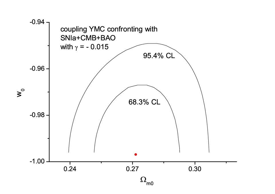
For the coupling model, there are three independently adjusted parameters $\gamma$, $\Omega_{m0}$ and $w_{0}$. In order to search for possible DE models in an extended domain, in particular, we will allow the coupling $\gamma$ to take negative values. For each fixed value of $\gamma$, we minimize $\chi^{2}$ with $\Omega_{m0}$ and $w_{0}$. We have done ten different values of $\gamma$, and the resulting values of $\chi^{2}_{min}$ for the corresponding sets of ($\gamma$, $\Omega_{m0}$ $w_{0}$) are listed in Table 1. It is seen that, as a function of $\gamma$, the minimum $\chi^{2}_{min}=542.790$ is attained at $\gamma=-0.015$, $\Omega_{m0}=0.2715$ and $w_{0}=-0.9969$. This $\chi^{2}_{min}$ is slightly smaller than that of the non-coupling and of the $\Lambda$CDM models. Table 1 also tells that, although the $\chi^{2}_{min}$ depends on $\gamma$, the dependence is not very strong.

Our previous work [16] did not search for the minimal $\chi^{2}$ with respect to the parameter $\gamma$ since it calculated only three different values of $\gamma$.

Figure 2 shows the C.L. curves with $\gamma=-0.015$ in the $(\Omega_{m0},w_{0})$ plane.

Thus the YMC model with a negative coupling $\gamma<0$ does a bit better than the latter two models in confronting the updated observations. We remark that this conclusion was partly hinted in the 3-loop YMC model, where the consideration was confined only to the limited region of $\gamma>0$ [16]. Note that $\gamma<0$ means a situation in which the matter is transferring energy into the YMC, and EoS $w_{0}$ will not cross over $-1$ [14]. Besides, in the far future when the scale factor is hundreds times the present one, the matter density $\rho_{m}$ will turn into negative, which would be a non-physical region. Thus, the model of a negative coupling is phenomenological and can not be infinitely extended into far future. In regards to the issue of coupling, we notice that a positive interaction is preferred in a study of dynamics of galaxy clusters with a coupling between dark energy and dark matter [33].

The $\chi^{2}$ analysis is effective in searching for the best-fit values of parameters within a given model. But for models with different number of parameters, one would expect $\chi^{2}_{min}$ decreases as the number of free model parameters increase. For model comparisons in this case, one can use other kinds of criteria for model selection, such as BIC [27], AIC [28], and $\chi^{2}_{min}/dof$ with the degree of freedom $dof=N-k$, whereas $N$ and $k$ are the number of data points and the dimension (number of independently adjusted parameters) of the statistical model, respectively. The BIC is defined as $BIC\equiv-2\ln{\cal L}_{max}+k\ln N\,$, where ${\cal L}_{max}$ is the maximum likelihood. In the Gaussian case, $\chi^{2}_{min}=-2\ln{\cal L}_{max}+constant$, so that the difference in BIC is given by $\Delta{\rm BIC}=\Delta\chi^{2}_{min}+\Delta k\ln N$. The AIC is defined as $AIC\equiv-2\ln{\cal L}_{max}+2k\,$, and the difference in AIC is given by $\Delta{\rm AIC}=\Delta\chi^{2}_{min}+2\Delta k$. We present the results for these three criteria in Table 2, which imply that the $\Lambda CDM$ is still favored due to its simplicity, whereas the coupling model is ranked last as it has most parameters.

In summary, using the $\chi^{2}$ analysis alone in confronting to the updated observational data of 557 SNIa +CMB+BAO, we find that the non-coupling YMC is favored over $\Lambda$CDM, and the coupling YMC with a negative $\gamma$ is the most favored. Taking into account of the dimension of a statistical model, $\Lambda$CDM is still simplest. Overall, YMC is as robust as $\Lambda$CDM. More observational data at higher redshifts in future are much desired to shed light on the issue of dark energy.

ACKNOWLEDGMENT: Y. Zhang’s research work has been supported by the CNSF No.11073018, SRFDP, and CAS. We would like to thank W. Zhao for many helpful discussions.

References

- [1] A. G. Riess et al., Astron. J. 116, 1009 (1998); A. G. Riess et al., Astron. J. 117, 707 (1999); A. G. Riess et al., Astrophys. J. 607, 665 (2004); S. Perlmutter et al., Nature 391, 51 (1998); S. Perlmutter et al., Astrophys. J. 517, 565 (1999); M. G. Peter et al., Astrophys. J. 509, 74 (1998); B. Schmidt, P.et al., Astrophys. J. 507, 46 (1998).
- [2] J. L. Tonry et al., Astrophys. J. 594, 1 (2003); R. A. Knop et al., Astrophys. J. 598, 102 (2003); J. B. Brian et al., Astrophys. J. 602, 571 (2004); S. Nobili et al., Astrophys. J. 700, 1415 (2009); P. Astier et al., Astron. Astrophys. 447, 31 (2006); W. M. Wood-Vasey et al., Astrophys. J. 666, 694 (2007); J. Guy et al., Astron. Astrophys. 523, A7 (2010); A. H. Jon et al., Astron. J. 136, 2306 (2008); K. Richard et al., Astrophys. J. Suppl. Ser. 185, 32 (2009); A. G. Riess et al., Astrophys. J. 659, 98 (2007);
- [3] C. L. Bennett et al., Astrophys. J. Suppl. Ser. 148, 1 (2003); D. N. Spergel et al., Astrophys. J. Suppl. Ser. 170, 377 (2007).
- [4] J. Dunkley et al., Astrophys. J. Suppl. Ser. 180, 306 (2009); E. Komatsu et al., Astrophys. J. Suppl. Ser. 180, 330 (2009).
- [5] N. A. Bahcall, J. P. Ostriker, S. Perlmutter, and P. J. Steinhardt, Science 284, 1481 (1999); M. Tegmark et al., Phys. Rev. D 69, 103501 (2004); M. Tegmark et al., Phys. Rev. D 74, 123507 (2006); C. P. Adrian et al., Astrophys. J. 607, 655 (2004); W. J. Percivalet al., Astrophys. J. 657, 51 (2007); B. A. Reid et al., Mon. Not. Roy. Astron. Soc. 404, 60 (2010).
- [6] L. Parker and A. Raval, Phys. Rev. D 60, 063512 (1999); L. Parker and D. A. T. Vanzella, Phys. Rev. D 69, 104009 (2004).
- [7] S. Weinberg, Arxiv :astro-ph/0005265, (2000); S. M. Carroll, Living Rev. Relativity. 4, 1 (2001); P. J. E. Peebles and B. Ratra, Rev. Mod. Phys. 75, 559 (2003).
- [8] T. Padmanabhan, Phys. Rept. 380, 235 (2003); E. J. Copeland, M. Sami, and S. Tsujikawa, Int.J.Mod.Phys.D 15, 1753 (2006).
- [9] B. Ratra and P. J. E. Peebles, Phys. Rev. D 37, 3406 (1988); P. J. E. Peebles and B. Ratra, Astrophys. J. 325, L17 (1988); C. Wetterich, Nuclear Physics B 302, 668 (1988); C. Wetterich, Astron. Astrophys. 301, 321 (1995); R. R. Caldwell, R. Dave, and P. J. Steinhardt, Phys. Rev. Lett. 80, 1582 (1998); I. Zlatev, L. Wang, and P. J. Steinhardt, Phys. Rev. Lett. 82, 896 (1999).
- [10] C. Armendariz-Picon, V. Mukhanov, and P. J. Steinhardt, Phys. Rev. D 63, 103510 (2001); C. Armendariz-Picon, V. Mukhanov, and P. J. Steinhardt, Phys. Rev. Lett. 85, 4438 (2000); T. Chiba, T. Okabe, and M. Yamaguchi, Phys. Rev. D 62, 023511 (2000).
- [11] R. R. Caldwell, Physics Letters B 545, 23 (2002); S. M. Carroll, M. Hoffman, and M. Trodden, Phys. Rev. D 68, 023509 (2003); R. R. Caldwell, M. Kamionkowski, and N. N. Weinberg, Phys. Rev. Lett. 91, 071301 (2003).
- [12] W. Hu, Phys. Rev. D 71, 047301 (2005); B. Feng, X. Wang, and X. Zhang, Phys.Lett. B 607, 35 (2005); W. Zhao and Y. Zhang, Phys. Rev. D 73, 123509 (2006); M. L. Tong, Y. Zhang, and Z. W. Fu, Class.Quant.Grav. 055006, 28 (2011).
- [13] Y. Zhang, General Relativity and Gravitation 34, 2155 (2002); Y. Zhang, General Relativity and Gravitation 35, 689 (2003); Y. Zhang, Chin. Phys. Lett. 20, 1899 (2003); Y. Zhang, Chin. Phys. Lett. 21, 1183 (2004); W. Zhao and Y. Zhang, Phys.Lett. B 640, 69 (2006); W. Zhao and Y. Zhang, Class.Quant.Grav. 23, 3405 (2006).
- [14] Y. Zhang, T. Y. Xia, and W. Zhao, Class.Quant.Grav. 24, 3309 (2007); W. Zhao, Int.J.Mod.Phys.D 18, 1331 (2009).
- [15] T. Y. Xia and Y. Zhang, Phys.Lett. B 656, 19 (2007).
- [16] S. Wang, Y. Zhang, and T. Y. Xia, J. Cosmol. Astropart. Phys. 10, 037 (2008); S. Wang and Y. Zhang, Phys.Lett. B 669, 201 (2008).
- [17] E.Elizalde, J.Lidsey, S.Norjiri, and S.Ordintsov, Phys.Lett.B 574, 1 (2003); C. G. Boehmer, T. Harko, Eur.Phys.J.C50, 423 (2007); F. A. Membiela, M. Bellini, NuovoCim.B123, 241 (2008); J. B. Jimenez, A. L. Maroto, JCAP 0903:016, (2009); D. V. Gal’tsov, arXiv:0901.0115.
- [18] S. L. Adler, Phys. Rev. D 23, 2905 (1981); S. L. Adler, Nuclear Physics B 217, 381 (1983); S. L. Adler and T. Piran, Rev. Mod. Phys. 56, 1 (1984).
- [19] M. Kowalski et al., Astrophys. J. 686, 749 (2008).
- [20] M. Hicken et al., Astrophys. J. 700, 1097 (2009).
- [21] R. Amanullah and et al., Astrophys. J. 716, 712 (2010).For The Supernova Cosmology Project, The numerical data of the full sample are available at http://supernova.lbl.gov/Union
- [22] E. Komatsu and et al., Astrophys. J. Supp. Ser. 192, 18 (2011).
- [23] W. J. Percival et al., Mon. Not. Roy. Astron. Soc. 401, 2148 (2010); W. J. Percival et al., Mon. Not. Roy. Astron. Soc. 381, 1053 (2007); W. J. Percival et al., Mon. Not. Roy. Astron. Soc. 337, 1068 (2002).
- [24] D. J. Eisenstein et al., Astrophys. J. 633, 560 (2005); W. J. Percival, Astrophys. J. 657, 51 (2007).
- [25] A. G. Riess et al., Astrophys. J. Supp. Ser.183, 109 (2009); Astrophys. J. 699, 539 (2009).
- [26] Gaztanaga E, Cabr¨¦A and Hui L, Mon. Not. Roy. Astron. Soc.399 1663 (2009).
- [27] G. Schwarz, Ann. Stat. 6, 461 (1978).
- [28] H. Akaike, IEEE Trans. Automatic Control 19, 716 (1974).
- [29] Y. Zhang, Phys.Lett. B 340, 18 (1994); Y. Zhang, Class.Quant.Grav. 13, 2145 (1996); Y. Zhang, Chin. Phys. Lett. 14, 237 (1997); Y. Zhang, Chin. Phys. Lett. 15, 622 (1998); Y. Zhang, Communications in Theoretical Physics 30, 237 (1998); Y. Zhang, Chin. Phys. Lett. 19, 1569 (2002).
- [30] W. Hao, J. Cosmol. Astropart. Phys. 1008:020, (2010).
- [31] S. Nesseris and L. Perivolaropoulos, Phys. Rev. D 72, 123519 (2005).
- [32] V. Sahni, T. Saini, A. Starobinsky, and U. Alam, JETP Letters 77, 201 (2003); U. Alam, V. Sahni, T. Deep Saini, and A. A. Starobinsky, Mon. Not. Roy. Astron. Soc. 344, 1057 (2003); V. Sahni, A. Shafieloo, and A. A. Starobinsky, Phys. Rev. D 78, 103502 (2008); M. L. Tong, Y. Zhang, and T. Y. Xia, Int.J.Mod.Phys.D 18, 797 (2009); M. L. Tong and Y. Zhang, Phys. Rev. D 80, 023503 (2009); W. Zhao, Int.J.Mod.Phys.D 17, 1245 (2008); M. Tong and H. Noh, Eur. Phys. J. C 71, 1586 (2011).
- [33] E. Abdalla, L. R. Abramo, J. C. C de Souza, Phys. Rev. D 82, 023508 (2010).