Asymmetric spatial structure of zero modes for birefringent Dirac fermions

It is well known that the Dirac Hamiltonian with topologically non-trivial mass terms allows for zero energy modes.[1, 2, 3, 4, 5, 6, 7, 8, 9] If there is a single zero energy mode, then this leads to the non-trivial phenomenon of quantum number fractionalization, e.g. charge as has been experimentally confirmed in one dimension in polyacetylene.[2, 10] More recently, there has been much interest in zero modes that can arise from topological defects in systems whose low energy excitations can be described using Dirac fermions.[11, 12, 13, 14, 15, 16, 17, 18, 19] Such modes are being studied intensely due to the possibility of their application in quantum computation.[20, 21, 22, 23]

In all of these examples, the zero modes arise as a consequence of a topological defect in the mass term of the Dirac Hamiltonian. We consider here the recently introduced model of birefringent fermions [24] and introduce a momentum space vortex in addition to a standard mass vortex. The low energy theory of birefringent fermions consists of four component massless fermions with two separate Fermi velocities $v_{0}(1\pm\beta)$ controlled by the parameter $0\leq\beta\leq 1$. Writing the low energy theory in Dirac form, the parameter $\beta$ multiplies terms in the kinetic energy not present in the regular Dirac Hamiltonian.

Our main result is that when there is an appropriate vortex (anti-vortex) in $\beta$ in addition to a mass vortex (anti-vortex) of the type introduced in Ref. 6 then the ratio of the characteristic lengthscales of the zero mode solutions in the presence of either a vortex or an anti-vortex may be tuned arbitrarily by $\beta$. Specifically, we find that finite $\beta$ breaks the symmetry present when $\beta=0$ between the zero mode solutions in the presence of a mass vortex and a mass anti-vortex. The zero mode solution in the presence of a vortex becomes more extended while with an underlying anti-vortex it becomes more localized. In the limit $\beta=0$ the model we consider displays the same physics as that discussed in Ref. 6. The type of vortex we consider here may also be of interest in a variety of systems whose low energy excitations can be described as Weyl fermions with multiple Fermi velocities, which have recently been the focus of a number of publications.[25, 26, 27, 28, 29, 30]

This paper is structured as follows. In Sec. II we recall the model of birefringent Dirac fermions and describe the vortex that we are considering. In Sec. III we find the zero energy modes associated with this vortex, and study a tight-binding lattice model to illustrate this physics numerically in Sec. IV. In Sec. V we discuss our results and conclude.

The model of birefringent fermions introduced in Ref. 24 has the feature that there are massless fermions near the Dirac points, but with two distinct Fermi velocities. This model may be obtained as the low-energy theory associated with spinless fermions at half filling in a particular tight binding model on a square lattice with a four site unit cell illustrated in Fig. 1.

The dispersion relation reads as

where $J_{\pm}=J_{0}(1\pm\beta)$, with $0\leq\beta\leq 1$. This dispersion leads to four equivalent Dirac points at the corners of the Brillouin zone: ${\mathbf{K}}_{\pm,\pm}=\left(\pm\frac{\pi}{2},\pm\frac{\pi}{2}\right)$. Labelling the four sites in the unit cell as $A$, $B$, $C$, and $D$ we can write the low energy theory in the form:

where $\psi_{k}^{T}=(c_{Ak},c_{Bk},c_{Ck},c_{Dk}),$ with $c_{Ik}$ a fermionic annihilation operator for a fermion with momentum $k$ which resides on sites $I=A,B,C,$ or $D$, and (setting $2J_{0}=1$)

We use a non-standard representation of the gamma matrices in which $\gamma_{0}=\sigma_{3}\otimes\sigma_{3}$, $\gamma_{1}=\sigma_{2}\otimes I_{2}$, $\gamma_{2}=\sigma_{3}\otimes\sigma_{2}$, $\gamma_{3}=-\sigma_{1}\otimes I_{2}$, and $\gamma_{5}=\gamma_{0}\gamma_{1}\gamma_{2}\gamma_{3}=-\sigma_{3}\otimes\sigma_{1}$. The matrices $\gamma_{0}$, $\gamma_{1}$, $\gamma_{2}$, $\gamma_{3}$ and $\gamma_{5}$ satisfy the Clifford algebra $\gamma_{\mu}\gamma_{\nu}+\gamma_{\nu}\gamma_{\mu}=2\delta_{\mu\nu}$.[31] The representation of the gamma matrices is four dimensional, which is the minimal dimension for a time-reversal invariant system of spinless Dirac fermions in two dimensions on a lattice.[32] By way of comparison, in graphene, the minimal representation is constructed with two sublattice degrees of freedom and two inequivalent Dirac points. In the present problem, on the other hand, there are four equivalent Dirac points, but the unit cell is comprised of four lattice points. The two Dirac cones with Fermi velocities $1\pm\beta$ suggest the problem may be written as a direct sum of two copies of two component massless Dirac fermions or Weyl fermions. [This possibility was recently considered and it was shown that one cannot have a Weyl fermion in this present scenario.[32]] The realization of Weyl fermions in a two dimensional lattice without broken time reversal symmetry is also prohibited by Nielsen-Ninomiya theorem.[33, 34] However in the limit $\beta=1$ there are two flat bands at zero energy and a two component Weyl fermion. Such a possibility was previously discussed in other contexts[35, 36] – nevertheless the Nielsen-Ninomiya theorem is respected there as well.

We now search for zero energy modes that satisfy $H_{m,\beta}\Psi=0$. The existence of a unitary operator, $\gamma_{0}$, such that $\{H_{m,\beta},\gamma_{0}\}=0$, ensures the spectral symmetry of the energy eigenstates of $H_{m,\beta}$. Moreover, one may find an anti-unitary operator $M=UK$, where $U$ is unitary and $K$ is the complex conjugation operator, which anticommutes with the Hamiltonian.[14] Noting that $\{i\gamma_{0}\gamma_{1},\gamma_{5},i\gamma_{0}\gamma_{3}\}$ are real and $\{i\gamma_{0}\gamma_{2},\gamma_{3},i\gamma_{0}\gamma_{5}\}$ are imaginary one finds $U=-i\gamma_{2}\gamma_{3}=\sigma_{1}\otimes\sigma_{3}$, in the “graphene representation”. A zero energy mode of $H_{\beta,m}$ must also, therefore be an eigenstate of $M$, which for the state $\Psi_{0}^{T}=(\psi_{1},\psi_{2},\psi_{3},\psi_{4})$ leads to the constraint $\psi_{1}=\pm\psi_{3}^{*}$, $\psi_{2}=\mp\psi_{4}^{*}$. The symmetry of the energy spectrum about zero implies that the zero energy mode should be robust against any weak local perturbation.

For further ease of calculation we redefine the components of $\Psi$ as $\Psi\to e^{\frac{i\pi}{4}\gamma_{0}}\Psi$ so that the eigenvalue equations for the zero energy mode take the form

where $\partial_{z}=\partial_{x}-i\partial_{y}=e^{-i\theta}\left(\partial_{r}-\frac{i}{r}\partial_{\theta}\right)$ and $\partial_{\bar{z}}=\partial_{x}+i\partial_{y}=e^{i\theta}\left(\partial_{r}+\frac{i}{r}\partial_{\theta}\right)$. $\Psi$ must be an eigenvector of $M$ as well as $H$, and choosing $\Psi$ to have eigenvalue -1 implies $\psi_{3}=-\psi_{1}^{*}$ and $\psi_{4}=\psi_{2}^{*}$ (we will discuss the choice that $M$ has eigenvalue $+1$ below). Under this constraint Eqs. (7) - (10) lead to only two independent equations:

To solve these equations we make use of an ansatz introduced in a different context by Ghaemi and Wilczek,[43] focusing first on Eq. (11). We make the ansatz

where $\phi_{2}$ and $\phi_{4}$ are real. In order to have a consistent solution, we must have that $v_{m}=v_{\beta}-1$. There is still some freedom in the choice of $l$ and $n$, depending on which terms are grouped together from Eq. (11) after the use of the ansatz in Eq. (13). The choice that allows either $l=n$ or $l\neq n$ and guarantees that the solution is single-valued is:

in which case we have the condition $l+n=2-v_{\beta}$. We now consider the asymptotic behavior of the solution of this equation at large and small $r$. In the large $r$ limit $\beta(r)\to\beta_{0}$ and $m(r)\to m_{0}$, and we can ignore $1/r$ terms. This leads to the solution as $r\to\infty$

where

is the inverse of the characteristic length scale for the zero mode in the presence of an anti-vortex and $A$ is a normalization constant. At small $r$, $\beta(r)\to 0$ and $m(r)\to 0$, in which case

In order that solution be normalizable near the origin, we require $l$, $n$ $\leq 0$, which implies $v_{\beta}\geq 2$.

We now consider the two cases $v_{\beta}$ odd and even separately. If $v_{\beta}$ is even, i.e. $v_{\beta}=2p$ for some integer $p$, then to satisfy Eqs. (14) and (15) subject to $l$, $n$ $\leq 0$ and $l+n=2-v_{\beta}=2(1-p)$ requires $p\geq 1$. There will be a solution with $l=n$ and $(2p-2)$ solutions with $l\neq n$. As far as the original equation we were trying to solve, Eq. (11), is concerned, solutions with $l\leftrightarrow n$ are equivalent, so there are in fact only $p-1$ solutions of Eq. (11) with $l\neq n$, and a total of $p$ zero mode solutions when $v_{\beta}=2p$ (which implies $v_{m}=2p-1$). When $v_{\beta}$ is odd, we can apply a similar analysis and find that for $v_{\beta}=2p+1$ (i.e. $v_{m}=2p$), then there are $p$ zero mode solutions. Hence to have a single zero mode with $M$ eigenvalue $-1$, we can either have $v_{\beta}=2$, $v_{m}=1$, or $v_{\beta}=3$, $v_{m}=2$.

In our solution above we assumed that the eigenvalue of $M$ is $-1$. If, on the other hand, we try to obtain a solution which is an eigenvector of $M$ with eigenvalue $+1$, then we find that we must have $v_{\beta}\geq 2$ and $v_{m}=v_{\beta}-1$, as before, and that there is no normalizable solution when $v_{\beta}=2$. However, there can be normalizable solutions when $v_{\beta}>2$, and in particular there is one normalizable solution when $v_{\beta}=3$, so that there are a total of $2$ normalizable zero modes (as would be expected from $v_{m}=2$ by the usual index theorem[3, 4]). We consider the situation with $v_{\beta}=2$, $v_{m}=1$ numerically in Sec. IV. It should be noted that the fact that the solution we obtained from Eqs. (11) and (12) has eigenvalue $-1$ for $M$ is not significant. We could have equally well found a normalizable solution with eigenvalue $+1$ and no normalizable solution with $-1$ when $v_{\beta}=2$ had we made a different redefinition of the fields before Eqs. (7) to (10), e.g. $\Psi\to e^{-\frac{i\pi}{4}\gamma_{0}}\Psi$.

We can also see that the mass anti-vortex is required in order to have normalizable solutions. If we set $m_{0}=0$, then we have an anti-vortex defect in the kinetic energy alone. At large distance, the solutions asymptote to a constant value as $r\to\infty$

leading to a non-normalizable solution. Note that additionally, when $m_{0}=0$ there is no gap in the spectrum. When $v_{\beta}>0$, there are no non-zero normalizable solutions for $\psi_{1}$.

Next we consider vortex configurations in $\beta$ and $m$, corresponding to negative integer values of $v_{\beta}$ and $v_{m}$, which will illustrate how the $\beta$ term modifies the usual solution to the mass vortex.[6] In this case, $\psi_{2}$ has no normalizable solutions. Nevertheless, one can obtain the zero energy mode by using the ansatz

and $\psi_{3}=-\psi_{1}^{*}$, associated with the $-1$ eigenvalue of $M$. The coupled differential equations for the zero mode then read as

Even though in the vicinity of the origin $\phi_{1}$ and $\phi_{3}$ behave identically to $\phi_{2}$ and $\phi_{4}$ respectively in Eq. (17), at large distances ($r\rightarrow\infty$)

where

is the inverse of the characteristic lengthscale for the zero mode in the presence of a vortex, and $B$ is a normalization constant. The lengthscale for the decay of the zero mode differs in this case from the lengthscale we found for the anti-vortex solution. The norm of the zero modes with $+1$ eigenvalue of $M$ in this situation grow with the system size when $v_{\beta}=-2$, $v_{m}=-1$.

In the limit $\beta_{0}=0$, the characteristic length scales for vortex and anti-vortex are the same, since the Hamiltonian associated with those two distinct topological defects are unitarily equivalent to each other. Namely, the vortex Hamiltonian may be obtained from the anti-vortex one via a unitary rotation by $\gamma_{5}$ in Eq. (6). However, this unitary equivalence breaks down for a birefringent Dirac Hamiltonian, leading to the distinct length scales found in Eqs. (16) and (22).

It is useful to present the zero modes in terms of the original spinor components $\psi_{k}$. In the presence of an anti-vortex the zero mode reads as $\psi^{T}_{0}=\left(0,\psi_{2},0,\psi^{*}_{2}\right)$. After unitary rotation by $U=U^{\dagger}_{1}U^{\dagger}_{2}U^{\dagger}_{3}$ one finds that the amplitudes of the zero energy mode with an underlying anti-vortex is finite only on the $B$ and $C$ sublattices. When there is an underlying vortex, the zero modes acquire a finite expectation value on the $A$ and $D$ sublattices. This can also be seen by noting that both the vortex and anti-vortex Hamiltonians anticommute with $\gamma_{0}$. Therefore the zero energy subspace ${\cal H}_{0}$ is invariant under $\gamma_{0}$ and it acts like an identity matrix in ${\cal H}_{0}$. Therefore all the zero energy states must be an eigenstate of $\gamma_{0}$ with eigenvalue $+1$ or $-1$. Since $\gamma_{0}=\sigma_{3}\otimes\sigma_{3}\equiv{\rm Diag}(1,-1,-1,1)$, the amplitude of the zero modes can be finite either on the $B$ and $C$ sublattices (anti-vortex) or $A$ and $D$ sublattices (vortex) in accordance with our explicit calculation.

The results we obtained regarding the zero modes in Sec. III are for a continuum theory. Previous studies[8, 44] have found that zero modes that are predicted from a continuum calculation are present in the spectrum of appropriate tight-binding models on a lattice. Given the complicated form of the vortex configuration we considered here, we check that the results we have obtained in the continuum limit carry over to the lattice. To do this we considered the lattice model introduced in Ref. 24 and introduced a $Z_{4}$ vortex (anti-vortex) with vorticity 2 in $\beta$ and a $Z_{4}$ vortex (anti-vortex) in $m$, as illustrated in Fig. 2 for antivortices in $\beta$ and $m$ centered on an A site.

We diagonalized the Hamiltonian on an $L\times L$ lattice and considered topological defects centered on A, B, C and D sites. We chose a vortex (anti-vortex) in both $\beta$ and $m$ with step-function spatial profile $f(r)\propto\theta(r-r_{0})$, with $r_{0}=3$ lattice spacings. Our results were qualitatively similar with topological defects centred on different sites, and we mainly display data for configurations of the type shown in Fig. 2 in which there is a topological defect centered on an A site. The spectrum as a function of system size is shown in Fig. 3 for $m_{0}=0.25$, $\beta_{0}=0.25$ for a topological defect centered on an A site. We see that there are two states which converge to zero energy, and a series of non-zero energy states in the gap – the continuum levels are visible at the top and bottom of the energy range. We can also see that there are small differences in the spectrum when there are vortex and anti-vortex configurations of the hopping.

Even though there is only one vortex (anti-vortex) on the lattice, there are two zero modes in the numerical spectrum as is expected for a finite size system with open boundary conditions.[44] The probability density of these states is localized at the centre of the lattice on the vortex (anti-vortex) and at the edge of the system. The integrated charge density averaged over all four possible locations of the topological defect (A, B, C or D) for the zero energy modes is illustrated in Fig. 4. We compare the cases $m_{0}=0.25$ and $\beta_{0}=0$ and $m_{0}=0.25$ and $\beta_{0}=0.75$, and it is quite evident that there is precisely half a charge localized around the centre of the system. The profiles also are in qualitative agreement with the spatial dependences derived in Sec. III. The antivortex solution with $\beta_{0}=0.75$ is considerably more localised than the vortex solution with the same $\beta_{0}$ and the solution when $\beta_{0}=0$, both at small $r$ and at larger $r\gtrsim 3r_{0}$ (see the inset to Fig. 4).

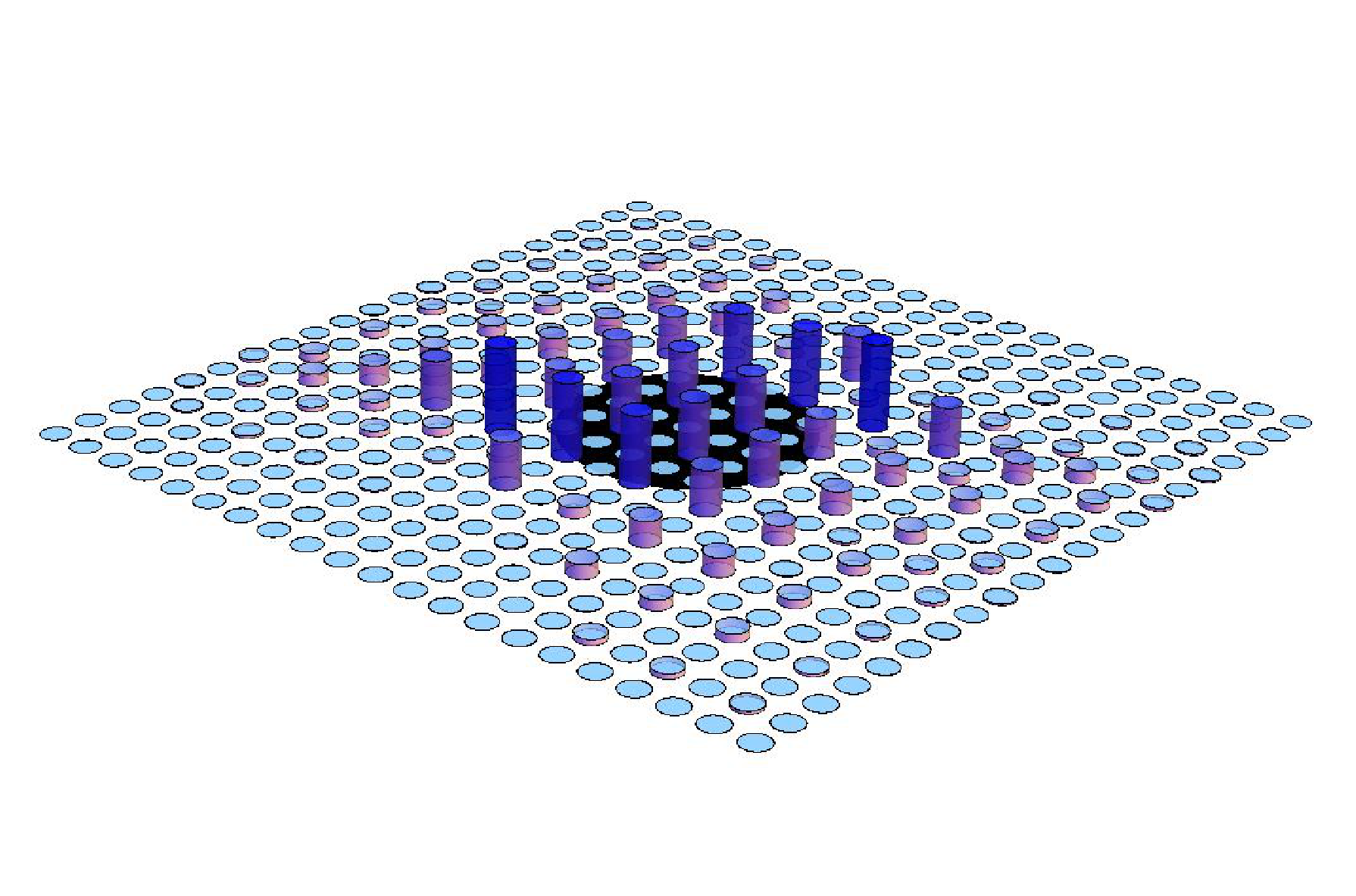
A feature of our analytical results is that the vortex and antivortex solutions have support on different sublattices. This is also borne out in our numerical results. We show the charge density for a vortex with $m_{0}=0.25$ and $\beta_{0}=0.75$ in Fig. 5 in which there is support for the state only on A and D sites, as deduced in Sec. III. We also confirmed that the state in the presence of an anti-vortex only has support on B and C sites.

In this paper we have studied the zero modes of birefringent Dirac fermions arising when there is an unusual vortex configuration which involves the kinetic energy as well as a mass term. This situation differs from the usual one in which there is fractionalization of non-interacting fermions in one or two dimensions due to a toplogical defect in some mass term.[45] In order to have a normalizable single-valued solution, there is a constraint on the allowed vorticity of the vortex (anti-vortex) in $\beta$ in that it winds one more time (in the same sense) as the vortex (anti-vortex) in $m$.

The effect of the topological defect in $\beta$ that we consider is to differentiate the spatial profiles of the zero modes associated with vortex and anti-vortex zero modes. The presence of the toplogical defect in the kinetic energy in addition to the mass leads to the unusual situation in which the length scale associated with the localized state at a vortex differs from the length scale associated with a state centered on an anti-vortex: the ratio of the two characteristic length scales is $(1+\beta_{0})/(1-\beta_{0})$ and so can be made arbitrarily large. The role of the vortex and the anti-vortex can be interchanged by changing the sign of $\beta$. As we emphasised in Sec. III the introduction of $\beta$ breaks the chiral symmetry that relates the vortex and antivortex Hamiltonians, allowing the possibility of differing zero mode solutions. It should be noted that the topological defect in $\beta$ does not affect the fractionalization associated with the topological defects, only the relevant lengthscales. We demonstrated this feature qualitatively through diagonalizing a lattice model and comparing the integrated charge density for the cases of $\beta_{0}=0$ and finite $\beta_{0}$.

The results we have obtained here have interest in a broader context than the particular problem we studied. Our work gives an example of a physical property that systems which exhibit birefringent massless fermionic excitations[26, 27, 28, 29, 30] can have that are unavailable for regular Dirac fermions (an other such example is birefringent Klein tunnelling[27]). The unusual occurrence of zero modes with different lengthscales (but not with associated fractionalization) was noted by two of us in Ref. 24 in the context of zero modes for birefringent Dirac fermions in the presence of a domain wall in a $\gamma_{0}$ mass term, and may be a generic feature of zero modes in birefringent Dirac systems. A situation in which there are two zero modes (hence there is no fractionalization) associated with a topological defect, but each has a differing lengthscale was also recently discussed by one of us in the context of graphene.[47]

The authors acknowledge helpful discussions with Claudio Chamon, Igor Herbut, Nazanin Komeilizadeh, Chi-Ken Lu and Joseph Thywissen. We acknowledge support from NSERC.

References

- [1] R. Jackiw and C. Rebbi, Phys. Rev. D 13, 3398 (1976).
- [2] W. P. Su, J. R. Schrieffer, and A. J. Heeger, Phys. Rev. Lett. 42, 1698 (1979); Phys. Rev. B 22, 2099 (1980).
- [3] R. Jackiw and P. Rossi, Nucl. Phys. B 190, 681 (1981).
- [4] E. J. Weinberg, Phys. Rev. D 24, 2669 (1981).
- [5] N. Read and D. Green, Phys. Rev. B 61, 10267 (2000).
- [6] C.-Y. Hou, C. Chamon, and C. Mudry, Phys. Rev. Lett. 98, 186809 (2007); C. Chamon, C.-Y. Hou, R. Jackiw, C. Mudry, S.-Y. Pi, and G. Semenoff, Phys. Rev. B 77, 235431 (2008).
- [7] R. Jackiw and S.-Y. Pi, Phys. Rev. Lett. 98, 266402 (2007); Phys. Rev. B 78, 132104 (2008).
- [8] B. Seradjeh, C. Weeks, and M. Franz, Phys. Rev. B 77, 033104 (2008).
- [9] B. Seradjeh, Nucl. Phys. B 805, 182 (2008).
- [10] N. Suzuki, M. Ozaki, S. Etemad, A. J. Heeger, and A. G. MacDiarmid, Phys. Rev. Lett. 45, 1209 (1980).
- [11] I. F. Herbut, Phys. Rev. Lett. 99, 206404 (2007); I. F. Herbut, Phys. Rev. B 81, 205429 (2010).
- [12] C. Chamon, R. Jackiw, Y. Nishida, S.-Y. Pi, and L. Santos, Phys. Rev. B 81, 224515 (2010).
- [13] Y. Nishida, L. Santos, and C. Chamon, Phys. Rev. B 82, 144513 (2010).
- [14] I. F. Herbut and C.-K. Lu, Phys. Rev. B 82, 125402 (2010).
- [15] C.-K. Lu and I. F. Herbut, Phys. Rev. B 82, 144505 (2010).
- [16] P. Hosur, P. Ghaemi, R. S. K. Mong, and A. Vishwanath, Phys. Rev. Lett. 107, 097001 (2011).
- [17] G. Möller, N. R. Cooper, and V. Gurarie, Phys. Rev. B 83, 014513 (2011).
- [18] G. Goldstein and C. Chamon, arXiv:1108.1734v2.
- [19] I. F. Herbut, Phys. Rev. B 85, 085304 (2012).
- [20] L. Fu and C. L. Kane, Phys. Rev. Lett. 100, 096407 (2008); F. Wilczek, Nature Phys. 5, 614 (2009); J. C. Y. Teo and C. L. Kane, Phys. Rev. Lett. 104, 046401 (2010).
- [21] A. R. Akhmerov, Phys. Rev. B 82, 020509(R) (2010).
- [22] D. A. Ivanov, Phys. Rev. Lett. 86, 268 (2001).
- [23] C. Nayak, S. H. Simon, A. Stern, M. Freedman, and S. Das Sarma, Rev. Mod. Phys. 80, 1083 (2008).
- [24] M. P. Kennett, N. Komeilizadeh, K. Kaveh, and P. M. Smith, Phys. Rev. A 83, 053636 (2011).
- [25] D. Bercioux, D. F. Urban, H. Grabert, and W. Häusler, Phys. Rev. A 80, 063603 (2009).
- [26] H. Watanabe, Y. Hatsugai, and H. Aoki, e-print arXiv:1009.1959.
- [27] Z. Lan, N. Goldman, A. Bermudez, W. Lu, and P. Ohberg, Phys. Rev. B 84, 165115 (2011).
- [28] Z. Lan, A. Celi, W. Lu, P. Ohberg, and M. Lewenstein, Phys. Rev. Lett. 107, 253001 (2011).
- [29] N. Goldman, D. F. Urban, and D. Bercioux, Phys. Rev. A 83, 063601 (2011).
- [30] B. Dóra, J. Kailasvuori, and R. Moessner, Phys. Rev. B 84, 195422 (2011).
- [31] Note that in Ref. 24 a Minkowski rather than Euclidean metric was used, which corresponds to slightly modified expressions for .
- [32] I. F. Herbut, Phys. Rev. B 83, 245445 (2011).
- [33] H. B. Nielsen and M. Ninomiya, Nucl. Phys. 185, 20 (1981).
- [34] F. D. M. Haldane, Phys. Rev. Lett. 61, 2015 (1988).
- [35] E. Dagotto, E. Fradkin, A. Moreo, Phys. Lett. 172, 383 (1986).
- [36] R. Shen, L. B. Shao, B. Wang, and D. Y. Xing, Phys. Rev. B 81, 041410(R) (2010); V. Apaja, M. Hyrkäs, and M. Manninen, Phys. Rev. A 82, 041402(R) (2010).
- [37] I. F. Herbut, V. Juričić, and B. Roy, Phys. Rev. B 79, 085116 (2009); B. Roy and I .F. Herbut 82, 035429 (2010).
- [38] E. Schonbrun and R. Piestun, Opt. Eng. 45, 028001 (2006).
- [39] W. S. Bakr, J. I. Gillen, A. Peng, S. Fölling, and M. Greiner, Nature 462, 74 (2009).
- [40] M. Aidelsburger, M. Atala, S. Nascimbène, S. Trotzky, Y.-A. Chen, I. Bloch, Phys. Rev. Lett. 107, 255301 (2011).
- [41] L. Tarruell, D. Greif, T. Uehlinger, G. Jotzu, and T. Esslinger, Nature 483, 302 (2012).
- [42] K. K. Gomes, W. Mar, W. Ko, F. Guinea, and H. C. Manoharan, Nature 483, 306 (2012).
- [43] P. Ghaemi and F. Wilczek, Phys. Scrip. T 146, 014019 (2012).
- [44] C. Chamon, C.-Y. Hou, R. Jackiw, C. Mudry, S.-Y. Pi, and A. P. Schnyder, Phys. Rev. Lett. 100, 110405 (2008).
- [45] There has been some study of momentum space vortices in the context of pseudospin magnetism in graphene,[46] but there has been no discussion of fractionalization in such a case.
- [46] H. Min, G. Borghi, M. Polini, and A.-H. MacDonald, Phys. Rev. B 77, 041407(R) (2008).
- [47] B. Roy, arXiv:1110.2584.