A fast direct solver for structured linear systems by recursive skeletonization Thanks: This work was supported in part by the National Science Foundation under grant DGE-0333389, by the U.S. Department of Energy under contract DEFG0288ER25053, and by the Air Force Office of Scientific Research under NSSEFF Program Award FA9550-10-1-0180.

Our treatment in this section follows that of [17]. Let $J=(1,2,\dots,N)$ be the index vector of a matrix $A\in\mathbb{C}^{N\times N}$. We assume that a tree structure $\tau$ is imposed on $J$ which is $\lambda+1$ levels deep. At level $l$, we assume that there are $p_{l}$ nodes, with each such node $J^{(l)}_{i}$ corresponding to a contiguous subsequence of $J$ such that

We denote the finest level as level $1$ and the coarsest level as level $\lambda+1$ (which consists of a single block). Each node $J^{(l)}_{i}$ at level $l>1$ has a finite number of children at level $l-1$ whose concatenation yields the indices in $J^{(l)}_{i}$ (Fig. 1).

The matrix $A$ is hierarchically block separable [17] if it is block separable at each level of the hierarchy defined by $\tau$. In other words, it is structured in the sense of the present paper if, on each level of $\tau$, the off-diagonal block rows and columns are low-rank (Fig. 2).

Such matrices arise, for example, when discretizing integral equations with non-oscillatory kernels (up to a specified precision).

Example 1. Consider the integral operator

where

is the Green’s function for the 2D Laplace equation, and the domain of integration is a square $B$ in the plane. This is a 2D volume integral operator. Suppose now that we discretize (4) on a $\sqrt{N}\times\sqrt{N}$ grid:

(This is not a high-order quadrature but that is really a separate issue.) Let us superimpose on $B$ a quadtree of depth $\lambda+1$, where $B$ is the root node (level $\lambda+1$). Level $\lambda$ is obtained from level $\lambda+1$ by subdividing the box $B$ into four equal squares and reordering the points $x_{i}$ so that each child holds a contiguous set of indices. This procedure is carried out until level $1$ is reached, reordering the nodes at each level so that the points contained in every node at every level correspond to a contiguous set of indices. It is clear that, with this ordering, the matrix corresponding to (6) is hierarchically block separable, since the interactions between nonadjacent boxes at every level are low-rank to any specified precision (from standard multipole estimates [22]). Adjacent boxes are low-rank for a more subtle reason (see §4 and Fig. 7).

Example 2. Suppose now that we wish to solve an interior Dirichlet problem for the Laplace equation in a simply connected 3D domain $\Omega$ with boundary $\partial\Omega$:

Potential theory [24] suggests that we seek a solution in the form of a double-layer potential

where

is the Green’s function for the 3D Laplace equation, $\nu_{y}$ is the unit outer normal at $y\in\partial\Omega$, and $\sigma$ is an unknown surface density. Letting $x$ approach the boundary, this gives rise to the second-kind Fredholm equation

Using a standard collocation scheme based on piecewise constant densities over a triangulated surface, we enclose $\partial\Omega$ in a box $B$ and bin sort the triangle centroids using an octree where, as in the previous example, we reorder the nodes so that each box in the hierarchy contains contiguous indices. It can be shown that the resulting matrix is also hierarchically block separable (see §4 and [21]).

We turn now to a discussion of the ID, the compression algorithm that we will use to compute low-rank approximations of off-diagonal blocks. A useful feature of the ID is that it is able to compute the rank of a matrix on the fly, since the exact ranks of the blocks are difficult to ascertain a priori—that is to say, the ID is rank-revealing.

Many decompositions exist for low-rank matrix approximation, including the singular value decomposition, which is well-known to be optimal [20]. Here, we consider instead the ID [10, 32, 48], which produces a near-optimal representation that is more useful for our purposes as it permits an efficient scheme for multilevel compression when used in a hierarchical setting.

Clearly, the ID compresses the column space of $A$; to compress the row space, simply apply the ID to $A^{\mathsf{T}}$, which produces an analogous representation $A=\tilde{P}\tilde{B}$, where $\tilde{P}\in\mathbb{C}^{m\times k}$ and $\tilde{B}\in\mathbb{C}^{k\times n}$.

Reasonably efficient schemes for constructing an ID exist [10, 32, 48]. By combining such schemes with methods for estimating the approximation error, we can compute an ID to any relative precision $\epsilon>0$ by adaptively determining the required rank $k$ [32]. This is the sense in which we will use the ID.

While previous related work [21, 35] used the deterministic $\mathcal{O}(kmn)$ algorithm of [10], we employ here the latest compression technology based on random sampling, which typically requires only $\mathcal{O}(mn\log k+k^{2}n)$ operations [32, 48].

Let $A\in\mathbb{C}^{N\times N}$ be a matrix with $p\times p$ blocks, structured in the sense of §2.1, and $\epsilon>0$ a target relative precision. We first outline a one-level matrix compression scheme:

1. 1.

   For $i=1,\dots,p$, use the ID to compress the row space of the $i$th off-diagonal block row to precision $\epsilon$. Let $L_{i}$ denote the corresponding row projection matrix.

2. 2.

   Similarly, for $j=1,\dots,p$, use the ID to compress the column space of the $j$th off-diagonal block column to precision $\epsilon$. Let $R_{j}$ denote the corresponding column projection matrix.

3. 3.

   Approximate the off-diagonal blocks of $A$ by $A_{ij}\approx L_{i}S_{ij}R_{j}$ for $i\neq j$, where $S_{ij}$ is the submatrix of $A_{ij}$ defined by the row and column skeletons associated with $L_{i}$ and $R_{j}$, respectively.

This yields precisely the matrix structure discussed in §2, following (1). The one-level scheme is illustrated graphically in Fig. 3.

The multilevel algorithm is now just a simple extension based on the observation that by ascending one level in the index tree and regrouping blocks accordingly, we can compress the skeleton matrix $S$ in (2) in exactly the same form, leading to a procedure that we naturally call recursive skeletonization (Fig. 4).

The full algorithm may be specified as follows:

1. 1.

   Starting at the leaves of the tree, extract the diagonal blocks and perform one level of compression of the off-diagonal blocks.

2. 2.

   Move up one level in the tree and regroup the matrix blocks according to the tree structure. Terminate if the new level is the root; otherwise, extract the diagonal blocks, recompress the off-diagonal blocks, and repeat.

The result is a telescoping representation

where the superscript indexes the compression level $l=1,\dots,\lambda$.

Example 3. As a demonstration of the multilevel compression technique, consider the matrix defined by $N=8192$ points uniformly distributed in the unit square, interacting via the 2D Laplace Green’s function (5) and sorted according to a quadtree ordering. The sequence of skeletons remaining after each level of compression to $\epsilon=10^{-3}$ is shown in Fig. 5, from which we see that compression creates a sparsification of the sources which, in a geometric setting, leaves skeletons along the boundaries of each block.

The computational cost of the algorithm described in the previous section is dominated by the fact that each step is global: that is, compressing the row or column space for each block requires accessing all other blocks in that row or column. If no further knowledge of the matrix is available, this is indeed necessary. However, as noted by [10, 21, 35, 37], this global work can often be replaced by a local one, resulting in considerable savings.

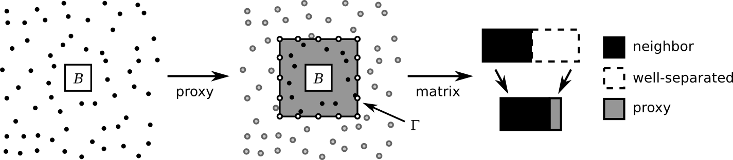
A sufficient condition for this acceleration is that the matrix correspond to evaluating a potential field for which some form of Green’s identities hold. It is easiest to present the main ideas in the context of Laplace’s equation. For this, consider Fig. 6, which depicts a set of sources in the plane. We assume that block index $i$ corresponds to the sources in the central square $B$. The $i$th off-diagonal block row then corresponds to the interactions of all points outside $B$ with all points inside $B$. We can separate this into contributions from the near neighbors of $B$, which are local, and the distant sources, which lie outside the near-neighbor domain, whose boundary is denoted by $\Gamma$. But any field induced by the distant sources induces a harmonic function inside $\Gamma$ and can therefore be replicated by a charge density on $\Gamma$ itself. Thus, rather than using the detailed structure of the distant points, the row (incoming) skeletons for $B$ can be extracted by considering just the combination of the near-neighbor sources and an artifical set of charges placed on $\Gamma$, which we refer to as a proxy surface. Likewise, the column (outgoing) skeletons for $B$ can be determined by considering only the near neighbors and the proxy surface. If the potential field is correct on the proxy surface, it will be correct at all more distant points (again via some variant of Green’s theorem).

The interaction rank between $\Gamma$ and $B$ is constant (depending on the desired precision) from standard multipole estimates [22, 23]. In summary, the number of points required to discretize $\Gamma$ is constant, and the dimension of the matrix to compress against for the block corresponding to $B$ is essentially just the number of points in the physically neighboring blocks.

Similar arguments hold for other kernels of potential theory including the heat, Helmholtz, Yukawa, Stokes, and elasticity kernels, though care must be taken for oscillatory problems which could require a combination of single and double layer potentials to avoid spurious resonances in the representation for the exterior.

The compressed representation (11) admits an obvious fast algorithm for computing the matrix-vector product $\mathbf{y}=A\mathbf{x}$. As shown in [17], one simply applies the matrices in (11) from right to left. Like the FMM, this procedure can be thought of as occurring in two passes:

1. 1.

   An upward pass, corresponding to the sequential application of the column projection matrices $R^{(l)}$, which hierarchically compress the input data $\mathbf{x}$ to the column (outgoing) skeleton subspace.

2. 2.

   A downward pass, corresponding to the sequential application of the row projection matrices $L^{(l)}$, which hierarchically project onto the row (incoming) skeleton subspace and, from there, back onto the output elements $\mathbf{y}$.

The representation (11) also permits a fast algorithm for the direct inversion of nonsingular matrices. The one-level scheme was discussed in §2. In the multilevel scheme, the system $S\mathbf{z}=\mathbf{y}$ in (3) is itself expanded in the same form, leading to the sparse embedding

To understand the consequences of this sparse representation, it is instructive to consider the special case in which the row and column skeleton dimensions are identical for each block, say $k$, so that the total row and column skeleton dimensions are $K\equiv K_{\mathrm{r}}=K_{\mathrm{c}}=pk$. Then, studying (3) first and assuming that $D$ is invertible, block elimination of $\mathbf{x}$ and $\mathbf{y}$ yields

where $\Lambda=(RD^{-1}L)^{-1}\in\mathbb{C}^{K\times K}$ is block diagonal. Back substitution then yields

In other words, the matrix inverse is

where

and

are all block diagonal, and

is dense. Note that $\mathcal{S}$ is equal to the skeleton matrix $S$ with its diagonal blocks filled in. Thus, (13) is a compressed representation of $A^{-1}$ with minimal fill-in over the original compressed representation (2) of $A$. In the multilevel setting, one carries out the above factorization recursively, since $\mathcal{S}$ can now be inverted in the same manner:

This point of view is elaborated in [17].

In the general case, the preceding procedure may fail if $D$ happens to be singular and (more generally) may be numerically unstable if care is not taken to stabilize the block elimination scheme using some sort of pivoting. Thus, rather than using the “hand-rolled” Gaussian elimination scheme of [16, 17, 35] to compute the telescoping inverse (14), we rely instead on the existence of high-quality sparse direct solver software. More precisely, we simply supply UMFPACK with the sparse representation (12) and let it compute the corresponding factorization. Numerical results show that the performance is similar to that expected from (14).

From §2.2, the cost of computing a rank-$k$ ID of an $m\times n$ matrix is $\mathcal{O}(mn\log k+k^{2}n)$. We will only consider the case of proxy compression, for which $m=\mathcal{O}(n_{l})$ for a block at level $l$, so the total cost is

The cost of applying $D^{(l)}$ is $\mathcal{O}(p_{l}n_{l}^{2})$, while that of applying $L^{(l)}$ or $R^{(l)}$ is $\mathcal{O}(p_{l}k_{l}n_{l})$. Combined with the $\mathcal{O}((p_{\lambda}k_{\lambda})^{2})$ cost of applying $S$, the total cost is

We turn now to the analysis of the cost of factorization using (14). At each level $l$, the cost of constructing $D^{-1}$ and $\Lambda$ is $\mathcal{O}(p_{l}n_{l}^{3})$, after which forming $\mathcal{D}^{(l)}$, $\mathcal{L}^{(l)}$, and $\mathcal{R}^{(l)}$ all require $\mathcal{O}(p_{l}n_{l}^{2})$ operations; at the final level, the cost of constructing and inverting $\mathcal{S}$ is $\mathcal{O}((p_{\lambda}k_{\lambda})^{3})$. Thus, the total cost is

which has complexity (15).

Finally, we note that the dimensions of $\mathcal{D}^{(l)}$, $\mathcal{L}^{(l)}$, $\mathcal{R}^{(l)}$, and $\mathcal{S}^{-1}$ are the same as those of $D^{(l)}$, $L^{(l)}$, $R^{(l)}$, and $S$, respectively. Thus, the total cost of applying the inverse, denoted by $T_{\mathrm{sv}}$, has the same complexity as $T_{\mathrm{mv}}$, namely (16).

In our UMFPACK-based approach, the estimation of cost is a rather complicated task, and we do not attempt to carry out a detailed analysis of its performance. Suffice it to say, there is a one-to-one correspondence between the “hand-rolled” Gaussian elimination approach and one possible elimination scheme in UMFPACK. Since that solver is highly optimized, the asymptotic cost should be the same (or better). For some matrices, it is possible that straight Gaussian elimination may be unstable without pivoting, while UMFPACK will carry out a backward-stable scheme. This is a distinct advantage of the sparse matrix approach although the complexity and fill-in analysis then becomes more involved.

An important issue in direct solvers, of course, is that of storage requirements. In the present setting the relevant matrices are the compressed sparse representation (12) and the factorization computed within UMFPACK. This will be (16) for the forward operator and, in the absence of pivoting, for the sparse factorization as well. If pivoting is required, the analysis is more complex as it involves some matrix fill-in and is postponed to future work.

We first consider the use of recursive skeletonization as a generalized FMM for the rapid computation of matrix-vector products.

In this section, we study the behavior of our algorithm as a fast direct solver. More specifically, we considered the interior Dirichlet problem for the Laplace and Helmholtz equations in 2D and 3D, recast as a second-kind boundary integral equation using the double-layer representation (8). Contour integrals in 2D were discretized using the trapezoidal rule, while surface integrals in 3D were discretized using Gaussian quadrature on flat triangles. In each case, we took as boundary data the field generated by an exterior point source; the error was assessed by comparing the field evaluated using the numerical solution via (8) against the exact field due to that source at an interior location. As a benchmark, we also solved each system directly using LAPACK/ATLAS, as well as iteratively using GMRES with matrix-vector products accelerated by the FMM.

References

- [1] P. R. Amestoy, I. S. Duff, J.-Y. L’Excellent, and J. Koster, A fully asynchronous multifrontal solver using distributed dynamic scheduling, SIAM J. Matrix Anal. Appl., 23 (2001), pp. 15–41.
- [2] E. Anderson, Z. Bai, C. Bischof, S. Blackford, J. Demmel, J. Dongarra, J. D. Croz, A. Greenbaum, S. Hammarling, A. McKenney, and D. Sorensen, LAPACK Users’ Guide, Society for Industrial and Applied Mathematics, Philadelphia, PA, USA, 3rd ed., 1999.
- [3] P. Beroza, D. R. Fredkin, M. Y. Okamura, and G. Feher, Protonation of interacting residues in a protein by a Monte Carlo method: Application to lysozyme and the photosynthetic reaction center of Rhodobacter sphaeroides, Proc. Natl. Acad. Sci. USA, 88 (1991), pp. 5804–5808.
- [4] J. Bremer, A fast direct solver for the integral equations of scattering theory on planar curves with corners, J. Comput. Phys., 231 (2012), pp. 1879–1899.
- [5] D. A. Case, T. E. Cheatham, T. Darden, H. Gohlke, R. Luo, K. M. Merz, A. Onufriev, C. Simmerling, B. Wang, and R. J. Woods, The Amber biomolecular simulation programs, J. Comput. Chem., 26 (2005), pp. 1668–1688.
- [6] S. Chandrasekaran, P. Dewilde, M. Gu, W. Lyons, and T. Pals, A fast solver for HSS representations via sparse matrices, SIAM J. Matrix Anal. Appl., 29 (2006), pp. 67–81.
- [7] S. Chandrasekaran, M. Gu, and T. Pals, A fast decomposition solver for hierarchically semiseparable representations, SIAM J. Matrix Anal. Appl., 28 (2006), pp. 603–622.
- [8] Y. Chen, A fast, direct algorithm for the Lippmann-Schwinger integral equation in two dimensions, Adv. Comput. Math., 16 (2002), pp. 175–190.
- [9] H. Cheng, W. Y. Crutchfield, Z. Gimbutas, L. F. Greengard, J. F. Ethridge, J. Huang, V. Rokhlin, N. Yarvin, and J. Zhao, A wideband fast multipole method for the Helmholtz equation in three dimensions, J. Comput. Phys., 216 (2006), pp. 300–325.
- [10] H. Cheng, Z. Gimbutas, P.-G. Martinsson, and V. Rokhlin, On the compression of low rank matrices, SIAM J. Sci. Comput., 26 (2005), pp. 1389–1404.
- [11] W. C. Chew, J.-M. Jin, E. Michielssen, and J. Song, Fast and Efficient Algorithms in Computational Electromagnetics, Artech House, Boston, MA, USA, 2001.
- [12] T. A. Davis, Algorithm 832: UMFPACK v4.3—an unsymmetric-pattern multifrontal method, ACM Trans. Math. Softw., 30 (2004), pp. 196–199.
- [13] T. A. Davis and I. S. Duff, An unsymmetric-pattern multifrontal method for sparse LU factorization, SIAM J. Matrix Anal. Appl., 18 (1997), pp. 140–158.
- [14] T. J. Dolinsky, J. E. Nielsen, J. A. McCammon, and N. A. Baker, PDB2PQR: an automated pipeline for the setup of Poisson-Boltzmann electrostatics calculations, Nucleic Acids Res., 32 (2004), pp. W665–W667.
- [15] H. R. Drew, R. M. Wing, T. Takano, C. Broka, S. Tanaka, K. Itakura, and R. E. Dickerson, Structure of a B-DNA dodecamer: conformation and dynamics, Proc. Natl. Acad. Sci. USA, 78 (1981), pp. 2179–2183.
- [16] A. Gillman, Fast Direct Solvers for Elliptic Partial Differential Equations, Ph.D. thesis, Department of Applied Mathematics, University of Colorado at Boulder, 2011.
- [17] A. Gillman, P. Young, and P.G. Martinsson, A direct solver with complexity for integral equations on one-dimensional domains, Front. Math. China, 7 (2012), pp. 217–247.
- [18] Z. Gimbutas and L. Greengard, FMMLIB: fast multipole methods for electrostatics, elastostatics, and low frequency acoustic modeling, in preparation.
- [19] Z. Gimbutas and V. Rokhlin, A generalized fast multipole method for nonoscillatory kernels, SIAM J. Sci. Comput., 24 (2003), pp. 796–817.
- [20] G. H. Golub and C. F. van Loan, Matrix Computations, The Johns Hopkins University Press, Baltimore, MD, USA, 3rd ed., 1996.
- [21] L. Greengard, D. Gueyffier, P.-G. Martinsson, and V. Rokhlin, Fast direct solvers for integral equations in complex three-dimensional domains, Acta Numer., 18 (2009), pp. 243–275.
- [22] L. Greengard and V. Rokhlin, A fast algorithm for particle simulations, J. Comput. Phys., 73 (1987), pp. 325–348.
- [23] L. Greengard and V. Rokhlin, A new version of the fast multipole method for the Laplace equation in three dimensions, Acta Numer., 6 (1997), pp. 229–269.
- [24] R. B. Guenther and J. W. Lee, Partial Differential Equations of Mathematical Physics and Integral Equations, Prentice-Hall, Englewood Cliffs, NJ, USA, 1988.
- [25] A. Gupta, WSMP: Watson Sparse Matrix Package. Part II—direct solution of general sparse systems, Technical report RC 21888, IBM T. J. Watson Research Center, 2000.
- [26] W. Hackbusch, A sparse matrix arithmetic based on -matrices. Part I: Introduction to -matrices, Computing, 62 (1999), pp. 89–108.
- [27] W. Hackbusch and S. Börm, Data-sparse approximation by adaptive -matrices, Computing, 69 (2002), pp. 1–35.
- [28] W. Hackbusch and B. N. Khoromskij, A sparse -matrix arithmetic. Part II: Application to multi-dimensional problems, Computing, 64 (2000), pp. 21–47.
- [29] W. W. Hager, Updating the inverse of a matrix, SIAM Rev., 31 (1989), pp. 221–239.
- [30] S. Kapur and V. Rokhlin, High-order corrected trapezoidal quadrature rules for singular functions, SIAM J. Numer. Anal., 34 (1997), pp. 1331–1356.
- [31] X. S. Li, An overview of SuperLU: algorithms, implementation, and user interface, ACM Trans. Math. Softw., 31 (2005), pp. 302–325.
- [32] E. Liberty, F. Woolfe, P.-G. Martinsson, V. Rokhlin, and M. Tygert, Randomized algorithms for the low-rank approximation of matrices, Proc. Natl. Acad. Sci. USA, 104 (2007), pp. 20167–20172.
- [33] Y. Liu, Fast Multipole Boundary Element Method: Theory and Applications in Engineering, Cambridge University Press, New York, NY, USA, 2009.
- [34] P.-G. Martinsson, Fast evaluation of electro-static interactions in multi-phase dielectric media, J. Comput. Phys., 211 (2006), pp. 289–299.
- [35] P.-G. Martinsson and V. Rokhlin, A fast direct solver for boundary integral equations in two dimensions, J. Comput. Phys., 205 (2005), pp. 1–23.
- [36] P.-G. Martinsson and V. Rokhlin, An accelerated kernel-independent fast multipole method in one dimension, SIAM J. Sci. Comput., 29 (2007), pp. 1160–1178.
- [37] P.-G. Martinsson and V. Rokhlin, A fast direct solver for scattering problems involving elongated structures, J. Comput. Phys., 221 (2007), pp. 288–302.
- [38] N. Nishimura, Fast multipole accelerated boundary integral equation methods, Appl. Mech. Rev., 55 (2002), pp. 299–324.
- [39] T. P. Pals, Multipole for Scattering Computations: Spectral Discretization, Stabilization, Fast Solvers, Ph.D. thesis, Department of Electrical and Computer Engineering, University of California, Santa Barbara, 2004.
- [40] V. Rokhlin, Rapid solution of integral equations of scattering theory in two dimensions, J. Comput. Phys., 86 (1990), pp. 414–439.
- [41] Y. Saad and M. H. Schultz, GMRES: A generalized minimal residual algorithm for solving nonsymmetric linear systems, SIAM J. Sci. Stat. Comput., 7 (1986), pp. 856–869.
- [42] M. F. Sanner, A. J. Olson, and J.-C. Spehner, Reduced surface: An efficient way to compute molecular surfaces, Biopolymers, 38 (1996), pp. 305–320.
- [43] O. Schenk and K. Gärtner, Solving unsymmetric sparse systems of linear equations with PARDISO, Future Gener. Comput. Syst., 20 (2004), pp. 475–487.
- [44] H. A. van der Vorst, Bi-CGSTAB: A fast and smoothly converging variant of Bi-CG for the solution of nonsymmetric linear systems, SIAM J. Sci. Stat. Comput., 13 (1992), pp. 631–644.
- [45] J.-G. Wei, Z. Peng, and J.-F. Lee, A fast direct matrix solver for surface integral equation methods for electromagnetic wave problems in , in Proceedings of the 27th International Review of Progress in Applied Computational Electromagnetics, Williamsburg, VA, USA, 2011, pp. 121–126.
- [46] R. C. Whaley, A. Petitet, and J. J. Dongarra, Automated empirical optimization of software and the ATLAS project, Parallel Comput., 27 (2001), pp. 3–35.
- [47] E. Winebrand and A. Boag, A multilevel fast direct solver for EM scattering from quasi-planar objects, in Proceedings of the International Conference on Electromagnetics in Advanced Applications, Torino, Italy, 2009, pp. 640–643.
- [48] F. Woolfe, E. Liberty, V. Rokhlin, and M. Tygert, A fast randomized algorithm for the approximation of matrices, Appl. Comput. Harmon. Anal., 25 (2008), pp. 335–366.
- [49] J. Xia, S. Chandrasekaran, M. Gu, and X. S. Li, Superfast multifrontal method for large structured linear systems of equations, SIAM J. Matrix Anal. Appl., 31 (2009), pp. 1382–1411.
- [50] L. Ying, G. Biros, and D. Zorin, A kernel-independent adaptive fast multipole algorithm in two and three dimensions, J. Comput. Phys., 196 (2004), pp. 591–626.