Formation, dynamics and stability of coreless vortex dipoles in phase-separated binary condensates
Abstract
We study the motion of the Gaussian obstacle potential created by blue detuned laser beam through a phase-separated binary condensate in pancake-shaped traps. For the velocity of the obstacle above a critical velocity, we observe the generation of vortex dipoles in the outer component which can penetrate the inner component. This is equivalent to finite, although small, transport of outer component across the inner component. In the inner component, the same method can lead to the formation of coreless vortex dipoles.
I Introduction
Generation of vortex dipoles in dilute Bose-Einstein condensates (BECs) when a superfluid moves past an obstacle with a velocity greater than a critical velocity (speed of sound locally) has been established by various numerical studies [1]-[5]. It has been established, both theoretically and numerically, that even the flow of the BEC below bulk sound speed can result in the flow velocity greater than the local sound speed at the equator of the obstacle. It implies that the critical velocity for the creation of vortex-antivortex pairs is lower than the bulk sound speed. Above this critical speed vortex-antivortex pairs are created periodically, resulting in an oscillatory drag force. This is due to the phase difference between the main flow and stationary wake behind the obstacle. Whenever this phase difference grows to a vortex-antivortex pair is created. Recently, Neely et al. [6] observed the generation of vortex dipoles in a pancake-shaped 87Rb condensate, when the condensate was moved past a Gaussian obstacle, created by blue-detuned laser beam, above critical velocity. Real time dynamics of single vortex line and vortex dipoles has also been studied experimentally [7]. The flow of the miscible binary and spinor condensates across a Gaussian obstacle potential has also been investigated theoretically in Refs.[8, 9, 10]. Vortex dipoles or vortex rings are also produced as one of the the decay products of dark solitons (a notch or density depression in the condensate with a phase slip of across it), due to the onset of a transverse instability in 2D and 3D geometries, namely snake instability. The decay of dark soliton into vortex rings has already been observed experimentally [11, 12]. In this context, it should be noted that motion of the obstacle across a 1D BEC generates grey solitons [13, 14, 15]. The snake instability is also responsible for the decay of ring soliton into a necklace of vortex dipoles [16].
In the present work, we study the flow of phase-separated binary condensates across a Gaussian obstacle numerically. We consider two experimentally realizable binary condensates: the first of these has 85Rb and 87Rb and the second has the two hyperfine states of 87Rb as the two constituent species. In both these condensates, one of the scattering length can be tuned by using magnetic Feshbach resonances [17, 18]. This allows us to choose the tunable scattering lengths values suitable for generation of coreless vortex dipoles. We observe the generation of vortex dipoles for the flow velocity greater than the critical velocity. In our simulations while moving the obstacle, its strength is continuously decreased. We consider two cases: (a) the obstacle laser potential, initially in the outer component, is moved towards the center, and (b) the obstacle laser potential, initially in the inner component, moves towards the interface of the binary condensate. With the successful realization of vortex dipoles in single component condensates using obstacle potential [6], the present studies give more than enough reasons to extend these experimental studies to binary condensates.
II Binary condensates and vortex dipoles
II.1 Meanfield description of binary condensates
The dynamics of binary condensate at K can be very well described by a set of coupled GP equations
| (1) |
in mean field approximation, where is the species index. Here , where is the mass and is the -wave scattering length, is the intra-species interaction, , where is the reduced mass and is the inter-species scattering length, is the inter-species interaction, and is the trapping potential experienced by th species. In the present work, we consider binary condensate consisting either of 85Rb and 87Rb for which . Furthermore, we also consider identical trapping potential for both the species, the total potential is then th species
| (2) |
where is the potential created by blue detuned laser beam, and and are anisotropy parameters. To rewrite the coupled GP equations in scaled units, define the oscillator length of the trapping potential
| (3) |
and consider as the unit of energy. We then divide the Eq.(1) by and apply the transformations
| (4) |
The transformed coupled GP equation in scaled units is
| (5) |
where , , and . From here on, we will represent the scaled quantities without tilde unless stated otherwise.
In pancake-shaped (highly oblate) traps, trapping frequency along axial direction is much greater than the radial directions, i.e., ; in which case Eq.(5) can be reduced to two dimensional form by substituting [19]. Here , the ground state wave function in axial direction. The reduced two dimensional form of coupled GP equation in pan-cake shaped traps is
| (6) | |||
where and . In the present work, we consider so that the ground state of the binary condensate is phase-separated. The ground states of the binary condensates in the phase separated domain have been studied in Refs.[20]-[27] In pancake-shaped traps the binary condensates has cylindrical interface separating the two components [26].
II.2 Vortex dipole trajectory in a single component condensate
The total velocity field experienced by each vortex in vortex dipole is the vector sum of two component fields. One of these fields is the velocity field generated on each vortex due to inhomogeneous nature of the condensate in the trapping potential. This inhomogeneity generated velocity field is responsible for the rotation of an off center vortex around the trap center [29, 28]. In addition to this, each vortex creates a velocity field varying inversely with the distance from its center, which is experienced by the other vortex of vortex dipole. If and are the locations of the positively and negatively charged vortices of the vortex dipole, respectively, then the total velocity field experienced by the positively charged vortex of the vortex dipole
| (7) |
where is the rotational frequency of a vortex with charge in the condensate. In terms of component velocities, the previous equation can be written as
| (8) |
This coupled set of differential equations describes the trajectory of the positively charged vortex of the vortex dipole. In the present work, we move the obstacle along -axis, leading to the generation of vortex dipole located symmetrically about -axis. Since is small (and positive) for the positively charged vortex of the vortex dipole at the instant of generation, one can neglect in first equation of coupled Eqs.8 to obtain
| (9) |
Eqs.9 imply that vortex initially to the left of the origin moves towards origin with increasing speed along positive -axis but decreasing speed along negative -axis. At , and beyond this vortex moves away from origin with decreasing speed along -axis but increasing speed along positive -axis. Near the origin , then the velocity of the vortex can be approximated as
| (10) |
In this case the velocity of the vortex is mainly induced one, and it moves with induced velocity towards positive direction. On the other hand if is too large, one can neglect term in Eq.8 to obtain
| (11) |
In this case, the velocity of the vortex is mainly due to the inhomogeneous nature of the condensate, resulting in the rotation with frequency . The transition between vortex induced velocity to inhomogeneity induced velocity occurs when , i.e., velocity along x-axis changes sign. From Eqs.8, it occurs at .
III Obstacle modified condensate density
In the phase separated domain of binary condensates, the species with lower repulsion energy forms a core and the other species forms a shell around it. For convenience, we identify the former and later as the first and second species, respectively. With this labelling, interaction energies and for equal populations this implies . There is large difference of the local coherence length when . This results in different density modifications for the two species when an obstacle beam is applied. The dynamics is most sensitive to the coherence length difference while the obstacle is crossing the interface layer of the binary condensate.
To analyze the density perturbations in presence of the obstacle beam, let be the radius of the inner species or the interface boundary. And, let be the radial extent of the outer species. In the absence of the obstacle beam, the chemical potential of first species is . Here, the second term is correction arising from the presence of the second species. The chemical potential of the second species is . Both of these are in scaled units. We consider the obstacle beam initially () located at and traversing towards the center with velocity . As it moves, its intensity is ramped down at the rate . The location of the beam at a later time is
| (12) |
and intensity of the beam is
| (13) |
where is the initial intensity of the obstacle beam. At the starting point, the total potential and the density of the outer species is zero around the center of the obstacle beam as is shown in Fig. 1(a).
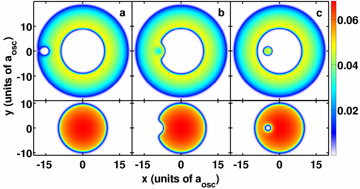
However, as it traverses the condensates with decreasing intensity, at some later time , . Density is then finite within the obstacle. For compact notations, hereafter we drop the explicit notation of time dependence while writing and .
III.1 Density modification at interface
As the obstacle beam approaches the interface, the intensity is weak to expel out the outer species. However, when the beam enters the inner species with any finite intensity , it is sufficient to make zero around the beam [see Fig. 1(a)]. The interface is modified and equipotential curve of the interface is
| (14) |
Around the center of the obstacle beam, , and the obstacle potential is
| (15) |
Hence from Eq.(14) the equipotential curve in the neighborhood of the obstacle beam is
| (16) |
where
Equipotential curve in the vicinity of the obstacle is thus modified into a circle with center at () and radius . In our numerical calculations, the Gaussian obstacle potential is quite narrow and . Retaining only the leading order terms in , the center is approximately located at and radius is
| (17) |
Sufficiently away from the obstacle and the obstacle potential is negligible. The equipotential curve then remains unchanged, . Thus an approximate piecewise expression of the equipotential curve is
This curve defines the interface geometry of the inner species in the TF approximation. Surface effects, however, smoothen the density profile around the meeting point of the two regions as is shown in Fig. 1(b). The obstacle beam is repulsive and expels the condensate around it such that bulk density is regained over a distance of one healing length.
III.2 Fully immersed obstacle beam
A critical requirement to form coreless vortices is complete immersion of the obstacle beam within . Based on the previous discussions, as the beam approaches the origin, the last point of contact between the beam and interface at lies along -axis. To determine the condition when complete immersion occurs, consider the total potential along -axis
| (18) | |||||
where, the Gaussian beam potential is considered upto the second order term. The expression is appropriate in the neighborhood of the beam and has one local minima and maxima each. There is also a global minima, however, it is not the correct solution as it lies in the domain where . Correct global minima is the one located at and associated with the harmonic potential. The obstacle is considered well immersed when the local minima is located at the interfacial radius . The local minima is a root of the polynomial
| (19) |
obtained from the condition . Here,
For the trapping potential parameters considered in the present work, all the three roots are real. The root corresponding to local minima is
| (20) |
where
and is a function of time as the obstacle potential is time dependent. However, for compact notations, like in and , hereafter we drop the explicit notation of time dependence while writing . Value of is real when it satisfies certain conditions [30] and these are met for the experimentally realizable parameters. The obstacle is then completely immersed when and let denote the time at which this condition is satisfied. Once the obstacle beam is well inside the inner species, within the beam is zero but is nonzero. It then forms a second interface layer, assisted by the obstacle beam, which embeds a bubble of the within . Recollect, the first interface layer is located at and it is where encloses . The second interface, unlike the one at , is a deformed-ellipse and label it as . It touches -axis at two points and is the one farther from the origin. From TF-approximation, the density of within is
| (21) |
where the subscript is to indicate the density is within . At , is in equilibrium with the bulk of , and let the number of atoms in the be , which can be calculated from .
Except for deviations arising from mean field energy, the second interface closely follows an equipotential surface. From the conditions of pressure balance at two interfaces
| (22) |
The first equation is valid all along the interface at . However, the second is derived at , but to a good approximation the condition is valid along as it is close to an equipotential surface. The density of the first species at (,0) is
| (23) |
Similarly density of second species at at (,0) is
| (24) |
Inside , where the obstacle potential is dominant, decays exponentially. Along the -axis
| (25) |
where, is the distance of the point measured from . Similarly the density of the second species just outside is
| (26) |
where is distance from but away from the obstacle beam, and is the penetration depth of the second species. In these expressions the penetration depth is
| (27) |
Based on the densities at the interface region, we can incorporate the interspecies interaction and calculate the effective potential of each species.
III.3 Obstacle assisted bubble
At a time after the obstacle is immersed in , the location and amplitude of the obstacle potential are
| (28) | |||||
| (29) |
Equilibrium TF within the obstacle potential at this instant of time is
| (30) |
This, however, is higher than the density distribution at , that is as the potential is lower. This is on account of two factors: first, the amplitude of the obstacle potential decreases with time; and second, the harmonic oscillator potential is lower at . The number of atoms, however, does not change from the value at unless there is a strong Josephson current. Density is thus below the equilibrium value once the obstacle beam is well within . This creates a stable bubble of assisted or trapped within the beam and is transported through the .
Departure of from the equilibrium is not the only density evolution within the beam. There is a progressive change of as the beam moves deeper into . At time , when the obstacle is completely immersed in the effective potential, experienced by , is larger than . So, is zero within the beam. However, if the rate of ramping is such that at a later time , while the beam is still within , there is a finite within the beam.
| (31) |
As the growth of is in its nascent stage, Eq. (30)is still applicable. Since for the condensate, in TF approximation both and can not be simultaneously non-zero. At the same time, is forbidden to migrate to the bulk due to the generated potential barrier in the region between interfaces and . To accommodate both and within the beam, the shape of interface is transformed to increase . So that is zero in certain regions within the beam where the condition is satisfied. This mechanism is responsible for obstacle assisted transport of across .
III.4 Obstacle induced density instability
The harmonic potential increases once the obstacle crosses origin, but the obstacle potential continues to decrease. A fine balance is achieved if
| (32) |
the dynamical rate of change of obstacle potential, is same in magnitude and opposite to the rate of change of the harmonic potential . It is, however, difficult to satisfy this condition across the entire obstacle potential as the Gaussian beam has has different profile than the oscillator trapping potential. But, the parameters may be tuned so that the condition is satisfied at the center of the beam, then
| (33) |
In the present case is a constant and the condition in Eq. (33) is satisfied only when the beam is at a specific point , then
| (34) |
Before reaching , the potential within the beam decreases, but increases after crossing it. At some point beyond , the total potential experienced by bubble can become greater than , resulting in an unstable bubble.
IV Stability of coreless vortex dipole
To analyze the energetic stability of coreless vortex dipoles in phase-separated binary condensates, we adopt the following ansatz for the wave function of inner and outer species
| (35) |
where is the location of the vortex dipole. With this choice of ansatz, the vortex dipole in the inner species is a normal vortex dipole. For simplicity of analysis, consider the trapping potential is purely harmonic, i.e.
| (36) |
Normalization yields the following constraints on and
| (37) |
and reduces the number of unknowns to two and . The energy of the binary condensate using the ansatz in Eq. (35) is
| (38) | |||||
In the same way, we can also determine the chemical potentials of the two species in terms of the same parameters. The stationary points of the energy function are the solutions of the coupled equations and . These equations are solvable analytically, but the solutions are lengthy and cumbersome. The solution of particular interest is the vortex dipole located along the -axis (). This is consistent with the observation that, regardless of the orientation, from the symmetry the axis passing through vortex dipole can be considered as the -axis. A rotation transformation is sufficient to achieve this. For the case considered, the energy extrema conditions simplify to equations
| (39) | |||||
For the sake of illustration, consider, , , , , , , , and . Call this set of parameters as parameters set b. The stationary points corresponding to minimum energy for this parameters set are .
IV.1 Coreless vortex dipole
To compare the energy of this normal vortex dipole with that coreless vortex dipole, consider that the cores of the vortices at and are filled with outer species. We approximate the cores as circular with a radius of , the coherence length of the inner species. We approximate the density profiles of the outer species within the cores with the TF distribution
| (40) |
where is the radial distance from the core of each vortex and antivortex. The above expression for is renormalized to obtain the modified value of , which in turn enables us to calculate the energy for the coreless vortex dipole. To obtain the analytic expression for energy, we integrate over the whole real space without excluding the core regions. The modified value of after the normalization is
| (41) |
With this approximation, the number of atoms of outer species embedded within the cores is
| (42) |
These contribute to the total energy through the potential and intra-species interaction energies. The energy contribution from the cores is then
| (43) | |||||
The total energy of the binary condensate with coreless vortex is
| (44) |
where is defined by Eqs. (38) and (41). For the parameter set b, the energy per particle [] is which is smaller than the value of obtained from Eqs. (37) and (38). This implies that coreless vortex dipole is energetically more favorable than normal vortex dipole with the percentage energy difference of .
The Gaussian form of the ansatz imposes limitations on the domain of applicability. But, the ansatz provide qualitative information on the stability coreless vortex dipoles. To relate to experimental realizations, consider 85Rb-87Rb binary condensate with , , and as the scattering length values and as the number of atoms. Here is tunable with magnetic Feshbach resonance [31]. With this set of parameters, the stationary state of 85Rb-87Rb binary condensate is just phase-separated. The trapping potential and obstacle laser potential parameters are same as those considered in Ref.[6], that is Hz, , , , and m. Hereafter we term this set of scattering lengths, number of atoms, and trapping potentials as set a. For this parameter set, in absence of the obstacle potential, the stationary point of minimum energy is . And, the difference in the energies per particle of the binary condensate with normal and coreless vortex dipoles is .
IV.2 TF approximation single vortex
As mentioned earlier, the applicability of the variational antsatz is limited to the weakly interacting domain. Experiments, however, mostly explore domains other than weakly interacting. To analyze stability in this domain, we resort to the TF approximation.
IV.2.1 Normal vortex
To simplify the analysis, consider a normal vortex located at the center of the inner species. For a normal vortex, the wave functions of the first or inner species in TF approximation is
| (45) |
Similarly, the wave function of the second or outer species is
| (46) |
here , , , and are the trapping potential, radius of the interface between inner and outer species, radial extent of outer species, and coherence length of inner species, respectively. The chemical potentials and are parameters of the calculations and obtained from inverting the normalization condition
| (47) | |||||
| (48) |
The total energy of the vortex with a normal vortex located at origin is
| (49) | |||||
The energy can be minimized under the constraint that and satisfy Eqs. (47-48) to completely determine the stationary state of binary condensate with a normal vortex at the origin.
IV.2.2 Coreless Vortex
For a coreless vortex, the wave functions of the two species in TF approximation are
| (50) | |||||
| (51) |
Normalizing the wave functions gives the constraint equations in terms of and as
| (52) | |||||
From the expressions, we can calculate the total energy of the system. It is a complicated expression which we refrain from writing. For the present case, it is perhaps sufficient to say, it is possible to obtain an analytical but cumbersome expression of total energy.
For the parameter set a with , binary condensate with the coreless vortex has lower energy than the one with normal vortex. This is evident from Fig.2 where the variation of total energy is shown as a function of .
However, the stability vanishes if one considers , , in set a. It is then the normal vortex which is energetically stable. This is evident form Fig.3.
These results are in very good agreement with numerical results. This TF analysis, albeit, is for single vortex clearly illustrates that depending upon the interaction parameters, a phase-separated binary condensate can either support coreless or normal vortex. It must be emphasized, the energy, chemical potentials, and interface radius obtained from the TF approximation are in very good agreement with numerical solution of coupled GP equations. For example, the numerical value of energy corresponding to Fig.3 is very close to the value from TF approximation.
IV.3 TF approximation with vortex dipole
We use the TF approximation to examine the stability of coreless vortices in the strongly interacting domain.
IV.3.1 Normal vortex dipole
Assume the vortex affects the density of the condensate only within the core regions. We then adopt the following ansatz for binary condensate with a normal vortex dipole at .
| (53) | |||||
| (54) |
The vortex dipole contributes mainly through the kinetic energy of , which may be approximated with the value of single species condensate given in Ref.[32]
| (55) |
Using these ansatz the number of atoms are
| (56) |
In a similar way, we can evaluate the energy of the entire condensate.
IV.3.2 Coreless vortex dipole
For coreless vortex dipole, we adopt the ansatz
| (57) | |||||
| (58) |
Using these ansatz the modified expressions for is
| (59) | |||||
We can also calculate the total energy of the system. The important change in is the inclusion of interface interaction energy . It arises from the interface interactions at the cores of the vortex and antivortex. Based on Ref. [21],
| (60) |
where is the pressure on the circumference of the cores and
| (61) |
As in the previous section, energy can be minimized with the constraint of the fixed number of atoms. For the parameters set a without obstacle potential, the coreless vortex dipole has lower energy than the normal vortex dipole and is shown in Fig. 4 for the vortex dipole located at .
For , , and rest of the parameters same as in parameter set a, condensate with the normal vortex dipole has lower energy than the one with coreless vortex dipole (see Fig. 5). These results are again in good agreement with the numerical results.
V Numerical results
For the numerical calculations, we again resort to experimentally realizable system and paramteres. We again work with the 85Rb-87Rb mixture and parameter set a introduced earlier. Recall, the values of paramteres in this set are , , and , Hz, , , , and m. As mentioned earlier, is tunable with magnetic Feshback resonance [31].
The transport of within the region of influence of is crucial to generate coreless vortices. As enters , it nudges and creates an interstice, which is occupied by . This is an outcome of the difference in coherence lengths (). The smaller of ensures that it recovers bulk value over shorter distances. It implies that it is comparatively more difficult to displace the than . As the obstacle reaches the interface with diminished strength, it is unable to displace , but not for due larger . This results in an inward protrusion of the interface, which detaches from the interface at a later time. For detachment to occur, it should be energetically favorable. The difference in coupled with ensures that the interstitial filling of is energetically lower, in other words energetically favorable. This is easily confirmed with imaginary time propagation of GP equation to obtain the stationary state geometry of the binary condensate with located inside as is shown in Fig. 1(c).
V.1 Motion of towards interface
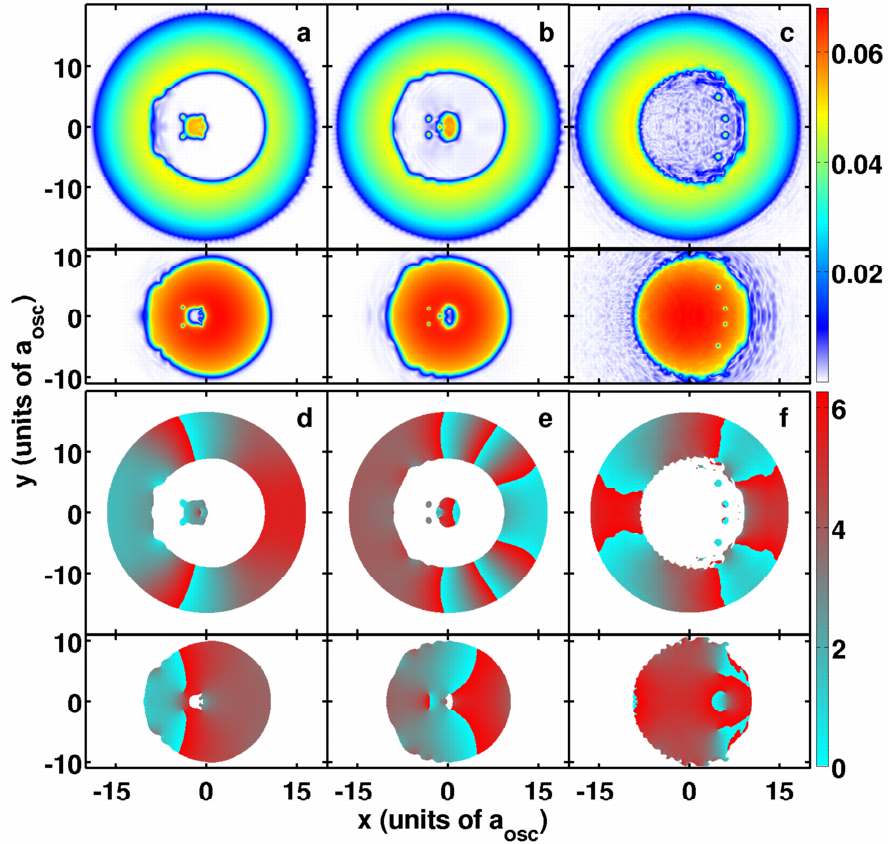
We first consider the motion of , initially located in the towards the interface. For this case, we consider 85Rb-87Rb binary condensate with parameter set a and of . The is initially located at and moves with the speed of m/s. It progressively decreases in strength and vanishes at . The obstacle creates a normal vortex dipole as it traverses . And, as approaches the interface, it transports the vortex dipole. Further motion of in the generates coreless vortices in the inner component. The formation of the coreless vortex dipole is shown in Fig. 6. The plots in the figure show both the density and phase distribution. From the phase plot, it is clear that the phase singularity of the vortex is associated with . And, from the density plot it is evident that the vortex-antivortex cores are filled with . One effect which precedes the seeding of coreless vortex is the indentation of the inner interface after it cleaves when the is fully immersed in . This may be explained in terms of the dynamical evolution around and analyzed in two different ways.
V.1.1 Inertia of
Just after the interface cleaves, when the is set into motion at , the due to inertia, does not follow initially. As a result at , neglecting the back flow of , outer species (along -axis) at is approximately same
| (62) |
here is time taken by the outer species to redistribute itself according to the displaced obstacle potential. As a result over a length , the density of inner species in TF approximation is
| (63) |
Hence inner flows into the above domain and replaces . The circular symmetry of coupled with motion along -axis ensures that the aforementioned process starts along -axis earlier; also the replacement of by takes place at the much faster speed as compared to the speed of the obstacle. This leads to creation of dimple on the inner interface.
V.1.2 Pressure balance
Let and be the location of the obstacle just after the interface cleaves and approximately circular inner interface centered around with radius , respectively. After time , let and be the location of the obstacle and inner interface, respectively. Assuming that has same radius as , i.e. , the points of intersection of and are
| (64) |
Thus the region defined as
| (65) |
with area
| (66) |
lies within but outside . Let and be the pressures exerted by inner and outer species on the left arc of region, respectively. The potential experienced by along the left arc of , which is approximately equal to harmonic trapping potential, does not change as the obstacle is moving away from this region, and so does the . The potential experienced by over , which is equal to sum total of harmonic trapping and obstacle potentials, decreases as the obstacle moves from to . In fact, as one moves from , where , to the along a curve with same sign of curvature as bounding arcs of region, the potential experienced by decreases. This leads to the redistribution of , i.e. it moves to the regions with weaker trapping potential. The redistribution will lead to which decreases as one moves along the aforementioned curve. This will lead to indentation of the inner interface. In our simulations, when the obstacle is moved, along -axis, from a point near the center towards the outer interface, indentation is suppressed. It confirms that this mechanism indeed aids the indentation of the interface.
V.2 Obstacle motion towards edge
In this case, we start with the stationary state solution of 85Rb-87Rb binary condensate for the parameters set a with obstacle laser potential maxima located at . The static solution in this case is shown in first column of Fig.7, which has roughly doughnut shaped density distribution of the outer species along with non-zero density in the circle of influence of the obstacle.
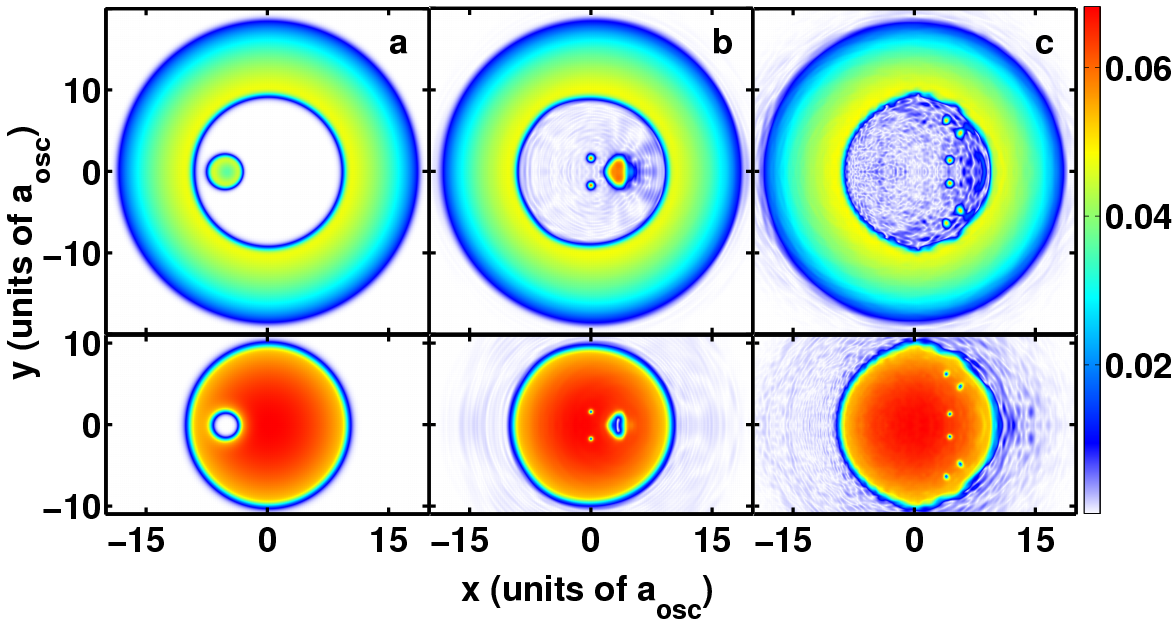
Such density distributions are prerequisite to create coreless vortices in the inner species. The obstacle is moved with a uniform speed of m/s, progressively decreases in strength, and finally becomes zero at . With this velocity, we observe the creation of triply charged coreless vortex dipole as is shown in last column of Fig.7. Singly and doubly charged vortex dipoles can be generated by moving the obstacle potential at lower velocities. For example, Fig.8 shows the singly charged coreless vortex dipole and the trajectory followed by it for the 85Rb-87Rb binary condensate with parameters set a. The obstacle laser potential moves from at to with the speed of m/s.

|
|
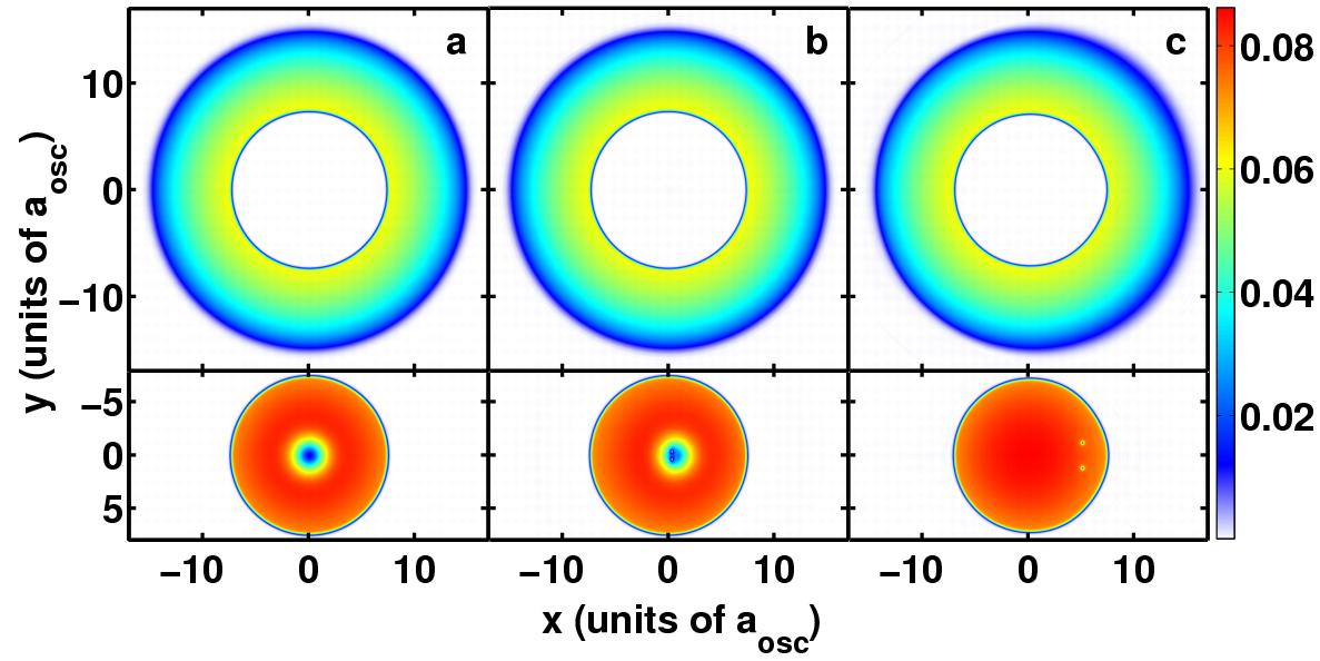
We also considered the 85Rb-87Rb with , , and the rest of the parameters same as those in parameter set a. The obstacle laser potential is initially located at origin . The stationary solution in this case is strongly phase separated (), and the circular region of influence of obstacle potential is devoid of atoms of outer component as is shown in first column of Fig.9. In our simulation, the obstacle potential potential traverses a distance of along x-axis with a speed of m/s. We observe that the vortex dipole generated in the inner component is a normal vortex dipole with empty core. This is consistent with the TF results shown in Fig. 5.
VI Conclusions
We have studied the motion of the Gaussian obstacle potential through a phase-separated binary condensate in pan-cake shaped traps. The motion of the obstacle leads to the generation of either coreless or normal vortex dipole depending upon the interaction parameters. The interaction parameters suitable for coreless vortex dipole can also be employed to have obstacle assisted transport of one species across another. We have used both a variational ansatz based method, applicable when , and TF approximation based method, applicable when , to analyze the energetic stability of coreless versus normal vortices. Our studies show that using Feshback resonances to tune one of the scattering length, e.g. scattering length of 85Rb in 85Rb-87Rb, it should be experimentally possible to create coreless vortices in phase-separated binary condensates.
Acknowledgements.
We thank S. A. Silotri, B. K. Mani, and S. Chattopadhyay for very useful discussions. The numerical computations reported in the paper were done on the 3 TFLOPs cluster at PRL. The work of PM forms a part of Department of Science and Technology (DST), Government of India sponsored research project.References
- [1] T. Frisch, Y. Pomeau, and S. Rica, Phys. Rev. Lett. 69, 1644 (1992).
- [2] T. Winiecki, J. F. McCann, and C. S. Adams, Phys. Rev. Lett. 82, 5186 (1999).
- [3] B. Jackson, J. F. McCann, and C. S. Adams, Phys. Rev. Lett. 80, 3903 (1998).
- [4] T. Winiecki et al., J. Phys. B 33, 4069 (2000).
- [5] C. Raman et al., Phys. Rev. Lett. 83, 2502 (1999). R. Onofrio et al., Phys. Rev. Lett. 85, 2228 (2000).
- [6] T. W. Neely, E. C. Samson, A. S. Bradley, M. J. Davis, and B. P. Anderson, Phys. Rev. Lett. 104, 160401 (2010).
- [7] D. V. Freilich, D. M. Bianchi, A. M. Kaufman, T. K. Langin, and D. S. Hall, Science 329, 1182 (2010).
- [8] H. Susanto, P. G. Kevrekidis, R. Carretero-Gonzalez, B. A. Malomed, D. J. Frantzeskakis, and A. R. Bishop, Phys. Rev. A 75, 055601 (2007).
- [9] Yu. G. Gladush, A. M. Kamchatnov, Z. Shi, P. G. Kevrekidis, D. J. Frantzeskakis, and B. A. Malomed, Phys. Rev. A 79, 033623 (2009).
- [10] A. S. Rodrigues, P. G. Kevrekidis, R. Carretero-Gonzalez, D. J. Frantzeskakis, P. Schmelcher, T. J. Alexander, and Yu. S. Kivshar, Phys. Rev. A 79, 043603 (2009).
- [11] B. P. Anderson, P. C. Haljan, C. A. Regal, D. L. Feder, L. A. Collins, C. W. Clark, and E. A. Cornell, Phys. Rev. Lett. 86, 2926 (2001).
- [12] Z. Dutton, M. Budde, C. Slowe, and L. V. Hau, Science 293, 663 (2001).
- [13] V. Hakim, Phys. Rev. E 55, 2835 (1997).
- [14] A. Radouani, Phys. Rev A 68, 043620 (2003); A. Radouani, Phys. Rev A 70, 013602 (2004).
- [15] R. Carretero-Gonzaleza, P. G. Kevrekidis, D. Frantzeskakis, B. A. Malomedd, S. Nandib, and A. R. Bishop, Mathematics and Computers in Simulation 74, 361 (2007).
- [16] G. Theocharis, D. J. Frantzeskakis, P. G. Kevrekidis, B. A. Malomed, and Y. S. Kivshar Phys. Rev. Lett. 90, 120403 (2003).
- [17] S. B. Papp, J. M. Pino, and C. E. Wieman, Phys. Rev. Lett. 101, 040402 (2008).
- [18] S. Tojo, Y. Taguchi, Y. Masuyama, T. Hayashi, H. Saito, and T. Hirano, Phys. Rev. A 82, 033609 (2010).
- [19] P. Muruganandam and S. K. Adhikari, Comp. Phys. Comm. 180, 1888 (2009).
- [20] Tin-Lun Ho, and V. B. Shenoy, Phys. Rev. Lett. 77, 3276 (1996).
- [21] E. Timmermans, Phys. Rev. Lett. 81, 5718 (1998).
- [22] P. Ao, and S. T. Chui, Phys. Rev. A 58, 4836 (1998).
- [23] R. A. Barankov, Phys. Rev. A 66, 013612 (2002).
- [24] B. Van Schaeybroeck, Phys. Rev. A 78, 023624 (2008).
- [25] M. Trippenbach, K. Goral, K. Rzazewski, B. Malomed, and Y. B. Band J. Phys. B 33, 4017 (2000).
- [26] S. Gautam and D Angom, J. Phys. B: At. Mol. Opt. Phys. 43, 095302 (2010).
- [27] S Gautam and D Angom, J. Phys. B: At. Mol. Opt. Phys. 44 025302 (2011).
- [28] A. A. Svidzinsky and A. L. Fetter, Phys. Rev. Lett. 84, 5919 (2000).
- [29] B. Jackson, J. .F. McCann, and C. .S. Adams Phys. Rev. A 61, 013604 (1999).
- [30] E. W. Weisstein, ”Cubic Formula.” From MathWorld–A Wolfram Web Resource.
- [31] S. L. Cornish, N. R. Claussen, J. L. Roberts, E. A. Cornell, and C. E. Wieman, Phys. Rev. Lett. 85, 1795 (2000).
- [32] Q. Zhou and H. Zhai, Phys. Rev. A 70, 043619 (2004).