Compressive and Noncompressive Power Spectral Density Estimation from Periodic Nonuniform Samples
Abstract
This paper presents a novel power spectral density estimation technique for band-limited, wide-sense stationary signals from sub-Nyquist sampled data. The technique employs multi-coset sampling and incorporates the advantages of compressed sensing (CS) when the power spectrum is sparse, but applies to sparse and nonsparse power spectra alike. The estimates are consistent piecewise constant approximations whose resolutions (width of the piecewise constant segments) are controlled by the periodicity of the multi-coset sampling. We show that compressive estimates exhibit better tradeoffs among the estimator’s resolution, system complexity, and average sampling rate compared to their noncompressive counterparts. For suitable sampling patterns, noncompressive estimates are obtained as least squares solutions. Because of the non-negativity of power spectra, compressive estimates can be computed by seeking non-negative least squares solutions (provided appropriate sampling patterns exist) instead of using standard CS recovery algorithms. This flexibility suggests a reduction in computational overhead for systems estimating both sparse and nonsparse power spectra because one algorithm can be used to compute both compressive and noncompressive estimates.
1 Introduction
Compressed sensing (CS) is a data acquisition strategy that exploits the sparsity or compressibility of a signal [1, 2, 3, 4]. Typically, a signal is defined to be sparse if its representation in an orthogonal basis contains only a few nonzero coefficients and is compressible if it can be well approximated by a sparse signal. In its simplest setting, CS proposes to sample a sparse discrete signal by acquiring inner product measurements , , where are the rows of a measurement matrix . In matrix notation, . Remarkably, CS asserts that can be accurately (if not exactly) reconstructed from the measurements even when the linear system of equations is underdetermined, provided satisfies certain conditions. When CS is applied to the problem of sampling continuous-time signals, it has been shown that the undersampling of finite length vectors translates into sub-Nyquist sampling rates, where CS provides the theoretical justification and tools to reconstruct the signal despite the spectral aliasing that can occur [5, 6, 7, 8].
In this paper, we study the problem of estimating the power spectral density (PSD) of a wide-sense stationary (WSS) random process within the context of a sub-Nyquist nonuniform periodic sampling strategy known as multi-coset (MC) sampling[9, 10, 11, 12, 13, 14, 15]. Because of its nonuniform periodic nature, MC sampling is closely related to CS,11 1 In fact, it can be formulated as a CS sampling strategy. and consequently, the proposed estimator easily incorporates and exploits CS theory. The estimator however applies broadly, and in particular, applies to cases where the PSD is not sparse.
For a fixed time interval and for a suitable positive integer , MC samplers sample an input signal at the time instants for , , where the time offsets are distinct, non-negative integers less than (). The strategy is depicted in Fig. 1. The sampling times are known collectively as the multi-coset sampling pattern and the sets are cosets of . Because is fixed throughout the paper, we simply refer to as the multi-coset sampling pattern instead of the actual sampling times. MC samplers are parameterized by , and and exhibit an average sampling rate of Hz. They are most easily implemented as multichannel systems as shown in Fig. 1 where channel shifts by seconds and then samples uniformly at Hz.
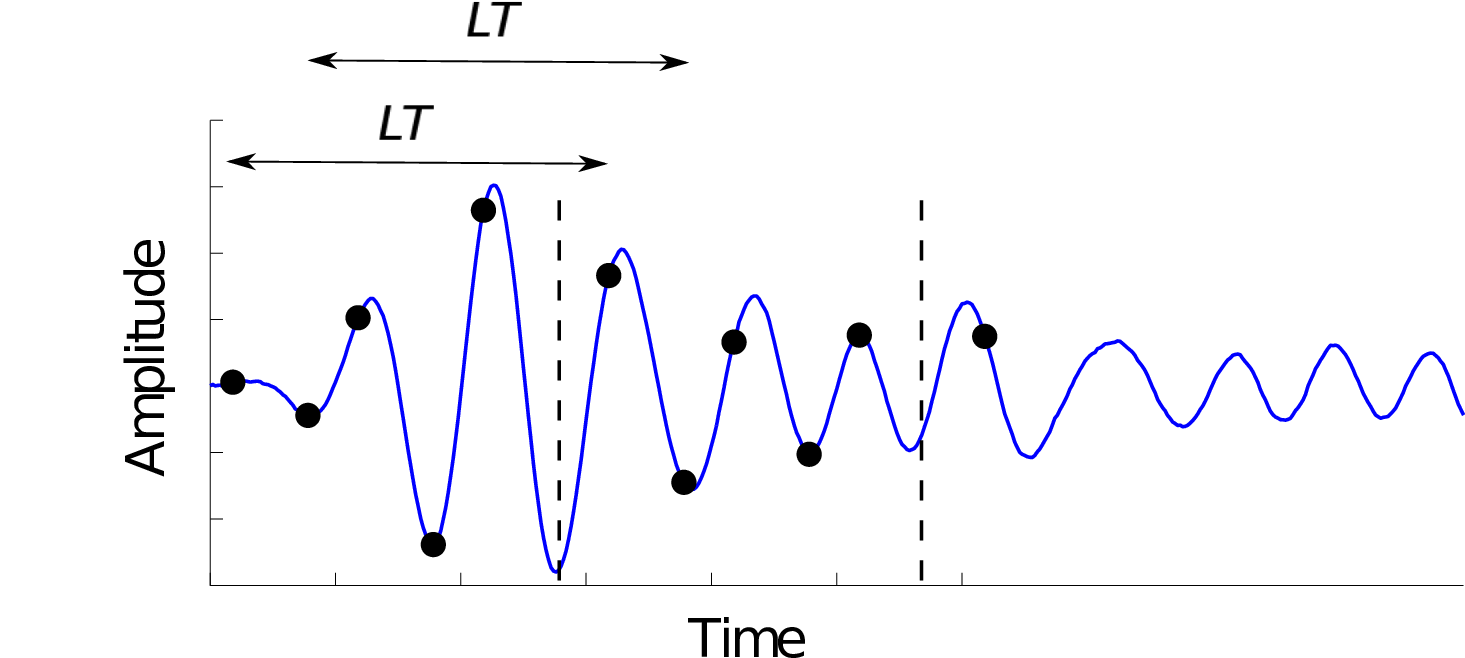

Here, we assume a multichannel MC sampler and propose a novel nonparametric PSD estimator based on the MC samples. The method estimates the average power within specific subbands of a WSS random process. Hence it produces piecewise constant estimates that are in contrast to those supported on a discrete frequency grid, e.g., the periodogram implemented using the discrete Fourier transform (DFT). Moreover, the estimator does not use passband filters to isolate subband signal components. Rather the estimator uses the spectral aliasing that occurs in each channel to underpin the formation of a linear system of equations whose solution is the PSD estimate of interest (see Section 2 for details).
We categorize the solutions to this linear system as either compressive or noncompressive depending upon whether CS is employed in the recovery of the estimate. Compressive estimates result from the application of CS theory and pertain to situations where the underlying power spectrum is sparse and the linear system of equations is underdetermined. Noncompressive estimates pertain to cases where the linear system is overdetermined (or determined) with the power spectrum’s sparsity being irrelevant. In both cases, the uniqueness of the recovered estimates depends on the choice of the sampling pattern (not all sampling patterns lead to unique solutions). Because of the special structure of the linear system, we show that in some cases compressive estimates can be computed using a non-negative least squares (NNLS) approach. This result is advantageous because in these cases it eliminates the necessity of using two separate algorithms to compute compressive and noncompressive estimates. (Note noncompressive estimates are normally computed as least squares solutions but can also be computed using NNLS; see Section 3.2 for details).
The proposed method also indicates the regions within the parameter space that allow for compressive and noncompressive estimates, and it illustrates the associated tradeoffs among quantities related to these parameters such as the estimator’s resolution or the number of MC channels. By comparing these tradeoffs one can gauge the benefit of appling CS theory in cases where the PSD is sparse. Perhaps surprisingly, the advantage of a compressive versus a noncompressive estimate is not simply an improved sampling rate, but rather improved tradeoffs [16]. For example, for a fixed spectral resolution, a compressive estimate might achieve the same accuracy as a noncompressive estimate but with a smaller number of channels. In addition, we show that both compressive and noncompressive estimates are statistically consistent and show that the noncompressive estimate is asymptotically efficient.
1.1 Related work
There is a growing literature in applying CS and other sub-Nyquist techniques to power spectrum estimation, most notably in the field of cognitive radios where there is a need to find underutilized bandwidth in a crowded spectrum [17, 18, 19, 20, 21, 22] Most pertinent to the present discussion, however, is the work of Ariananda, Leus and Tian [19, 20, 18]. These papers also address the problem of PSD estimation from sub-Nyquist samples specifically incorporating CS-based sampling systems (including MC sampling). Notwithstanding similar goals and approaches, the estimator proposed here differs in two significant aspects. First, their method estimates the cross-correlations of the MC sample sequences and then recovers an estimate of the auto-correlation sequence of the input random process (from which they form a periodogram estimate of the PSD). In contrast, the method described here directly recovers a piecewise constant estimate from the MC cross-correlation estimates. The main difference being that Araiananda et al. estimate samples of the PSD whereas we estimate the average power within subbands. An implication of this difference is that the method of Ariananda et al. is more computationally expensive: their method requires the formation of a large matrix in the construction of their measurement matrix; in contrast, we do not require the construction of this large matrix for our smaller measurement matrix. Second, we treat the compressive case and address the statistical nature of our estimator (specifically taking into account the finite availability of data), while Ariananda et al. do not.
1.2 Main contribution
In short, the paper’s main contribution is the development of a new nonparametric, statistically consistent, piecewise constant PSD estimator based on sub-Nyquist MC samples. When the underlying PSD is sparse, it seemlessly incorporates CS theory, letting the resulting compressive estimator exhibit better parametric tradeoffs compared to their noncompressive counterparts. Moreover, when a suitable sampling pattern exists, a NNLS approach can be used to compute compressive estimates, suggesting a possible savings in computational overhead for systems estimating sparse and nonsparse power spectra.
2 A PSD approximation from multi-coset samples
In this section, we derive a piecewise constant PSD approximation assuming full knowledge of the MC sequences. This approximation serves as the motivation and model for the noncompressive and compressive estimators derived in Sections 3. In Section 4, we present three examples illustrating the character and properties of the estimators.
2.1 PSD approximation
Let be a real, zero-mean, WSS random process with autocorrelation function , . The Fourier transform (FT) of is the PSD of [23].
The PSD quantifies the power in any given spectral band of and is a second order description of the random process. Because is real and symmetric, is also real and symmetric. Throughout the paper, we assume is a band-limited process, meaning that vanishes for rad/s [23, p. 376]. For the MC sampling, we set thereby referencing the average system sampling rate to the Nyquist rate .
To estimate using MC samples, we examine the cross-correlations of the output sequences . Let and denote two channels indices, then
| (1) |
where the third step follows from the wide-sense stationarity of and the substitution . From (1), we see that the cross-correlation function is equivalent to shifting the auto-correlation function by and then uniformly sampling it at Hz. These operations imply the following discrete time Fourier transform (DTFT) pair for and ,
| (2) | ||||
where the relation follows from the shifting and sampling properties of the DTFT [24, p. 98, 117]. The summation limits are finite for a given because is assumed band-limited. (Here we also assume is even.)
The phase shift in (2) arises from the time shifts introduced in the individual channels. For our purposes, however, this phase shift needs to be removed. This can be accomplished by shifting the sequences by an amount equal to, but opposite, the initial delays (see Fig. 2). Mathematically, this step can be expressed as
| (3) |
where denotes convolution and , are the impulse responses of ideal fractional delay filters [25]. These filters are “fractional” in the sense that the time shifts are a fraction of the sampling period . For simplicity, we assume ideal fractional delay filters throughout the paper. We note however that there is a large literature concerning the design and analysis of digital fractional delay filters (see [25] and the references wherein) ranging from highly accurate and computationally expensive filters to less accurate and computationally inexpensive ones. The choice of design is largely application dependent and a detailed analysis of the impact of imperfect fractional delay filters and is beyond the scope of this paper.

By examining the cross-correlation functions , we see that the fractional delays indeed delay by seconds.
| (4) | ||||
| (5) |
where the second step follows from (3), , and denotes the impulse of an ideal fractional delay filter with delay seconds.
Equation (5) also implies that the DTFT of is the DTFT of multiplied by . Thus, by multiplying the frequency domain component in (2) by , we obtain the following inverse DTFT relation
| (6) |
Evaluating both sides of this equation at produces a linear system of equations over the set of all pairs of channels:
| (7) |
This linear system is the basis for our estimator. For a given , equals the average power of the process in the spectral subband . Hence the set forms a piecewise constant approximation to . Its resolution equals the width of the piecewise constant segments ( Hz) and is inversely proportional to , the parameter determining the period of the nonuniform samples. Larger implies finer resolution; smaller implies coarser resolution. The left hand side of (7) is a weighted sum of the total average power of . In Section 3, we propose a statistical estimator based on this approximation that uses only a finite number of multi-coset samples. Like the approximation , the estimator is piecewise constant and thus does not estimate PSD amplitudes at specific frequencies like standard parametric techniques or periodiogram estimates implemented using the DFT.
Letting index the combinations22 2 In actuality, the total number of pairs is , but each of the cases where contributes a row of ones to . Thus to avoid the row dependency, only a single row of ones is included in . of pairs , we can express (7) in matrix notation,
| (8) |
where , and
| (9) |
for , , and . The number of equations in this linear system can be doubled by separating and into their real and imagery parts:
| (10) |
where and have dimensions and , respectively.
To calculate the PSD approximation, one would compute the set of cross-correlation values for all pairs and solve (10) for . Here we briefly consider two types of solutions, deferring a more detailed discussion until after the estimator is presented in Section 3 (see in particular Sections 3.2 and 3.3). First, we consider least squares solutions when is full rank (rank ) and (10) is overdetermined. Such solutions are referred to as noncompressive. Second, we consider CS solutions when (10) is underdetermined and is sparse in the sense that only a few of its entries are nonzero. These solutions are termed compressive.
The existence of a unique least squares solution depends on the (column) rank of which in turn depends on the sampling pattern . In particular, a sampling pattern must be chosen such that has rank (implying that , or equivalently, that the number of rows of is greater than or equal to the number of columns). In Section 3.2, we discuss two methods for constructing sampling patterns that produce full rank , but given such a sampling pattern, the unique least squares solution is
| (11) |
where denotes the norm, equals the pseudoinverse of , and the subscript NC indicates that the approximation is noncompressive. If and is nonsingular, we simply have .
Now, suppose is spectrally sparse, i.e., suppose its support has Lebesgue measure that is small relative to the overall bandwidth. In addition, suppose such that (10) is an underdetermined linear system of equations. Then from a CS perspective, is the sparse vector of interest that is to be recovered from the linear measurements , and is a (subsampled Fourier) measurement matrix. The vector is sparse because its entries represent the average power of in the subbands and is presumed to be sparse. In this situation, a host of CS recovery algorithms may be used to compute compressive approximations provided an appropriate sampling pattern and a sufficient number of measurements for a given level of sparsity (see e.g., [26, 27, 28]). For example, for a suitable sampling pattern, the convex optimization problem
| (12) |
would yield a compressive approximation if measurements were acquired [29], where denotes the norm and denotes the number of nonzero entries in . In Section 3.3, we further exploit the structure of this linear system and advocate an algorithm that does not require an explicit sparsity constraint in the recovery procedure.
3 Proposed multi-coset PSD estimator
The above PSD approximation is predicated on full knowledge of the output sequences , or equivalently, on having access to an infinite amount of data (an infinite number of multi-coset samples). In this section, we derive and characterize an estimator based on (8) that explicitly accounts for the finite availability of data.
3.1 PSD estimation
Again, let by a real, band-limited, zero-mean WSS random process with PSD . We observe over a finite duration interval and hence model the observed signal as a windowed version of :
| (13) |
where
| (14) |
The MC samples of the windowed process are
| (15) | ||||
for and , where equals the number of samples acquired per channel during the second observation interval. (Here is assumed to be an integer.) The fractionally delayed samples are (c.f. (3))
| (16) |
where again signifies the number of samples33 3 A perfect fractional delay filter has an infinite impulse response and thus the sequence has, strictly speaking, infinite duration. However, in (16) we only consider output samples , . We do not include another windowing operation because will be finite for any practical, realizable filter..
Let and denote the indices of two channels. Then, given and , the cross-correlation function can be estimated by the sample correlation
| (17) |
for . Mimicking the standard derivation of a periodogram (see e.g. [30, p.321]), we find the DTFT of to be
| (18) |
where and are the DTFT of and respectively. The transform may be further decomposed in terms of and where
| (19) | ||||
Specifically, for , we have from (15) and (16) that
| (20) | ||||
Because is time limited, it cannot, strictly speaking, be band-limited. However, for sufficiently long windows it is reasonable to assume that the vast majority of the energy of lies within the band , i.e., it is reasonable to assume that with sufficiently long windows is essentially band-limited to the same band as . With this assumption, one period of is well approximated by the finite summation,
| (21) |
Substituting (21) for in (18) (along with a corresponding expression for ) and evaluating the inverse DTFT at zero yields
| (22) |
where is shorthand notation for .
We observe that for , the integrands, , are periodogram estimates of disjoint subbands of , and the corresponding integrals
| (23) |
are estimates of the power within these subbands. The set thus constitutes a piecewise constant estimate of at resolution .
In contrast, the cross terms in (22) (i.e., terms for which ) asymptotically approach zero as , or equivalently , grows large. To see this, rewrite the integrand in (22) as
| (24) | ||||
where is the FT of the rectangular window , is the FT of appropriately defined (see [23, p. 416]), and
As , approaches a delta function [31, p. 280]; however because of the factors , the integrals approach zero as for .
Because of this fact, we choose to approximate using only the terms in (22)
| (25) |
Letting index all pairs , we arrive at an empirical counterpart to (8)
| (26) |
where
| (27) |
for , , and . Similar to (10), we can double the number of equations by separating the real and imagery parts of and :
| (28) |
where and is defined in (10). In this equation, is the PSD estimator we wish to solve for.
3.2 Noncompressive solutions (overdetermined case)
A unique least squares solution to (28) exists if has full column rank, i.e., . Full rank implies , or that the system is overdetermined (here we treat a determined system as a special case of the overdetermined one). In this case, a noncompressive estimate can computed using the pseudoinverse
| (29) |
where is the pseudoinverse of . A solution of this type is noncompressive because it does not rely on CS theory, and in particular, it does not require to be sparse.
For a fixed , a full rank requires (i) choosing large enough such that and (ii) choosing a sampling pattern such that . The first condition is required since implies , regardless of the sampling pattern. The second condition is necessary since there exists sampling patterns that lead to having a non-empty nullspace even if , meaning that the least squares solution is no longer unique. Section 3.4 discusses the tradeoff between and imposed by the first condition assuming the second condition is met. Here we address the second condition.
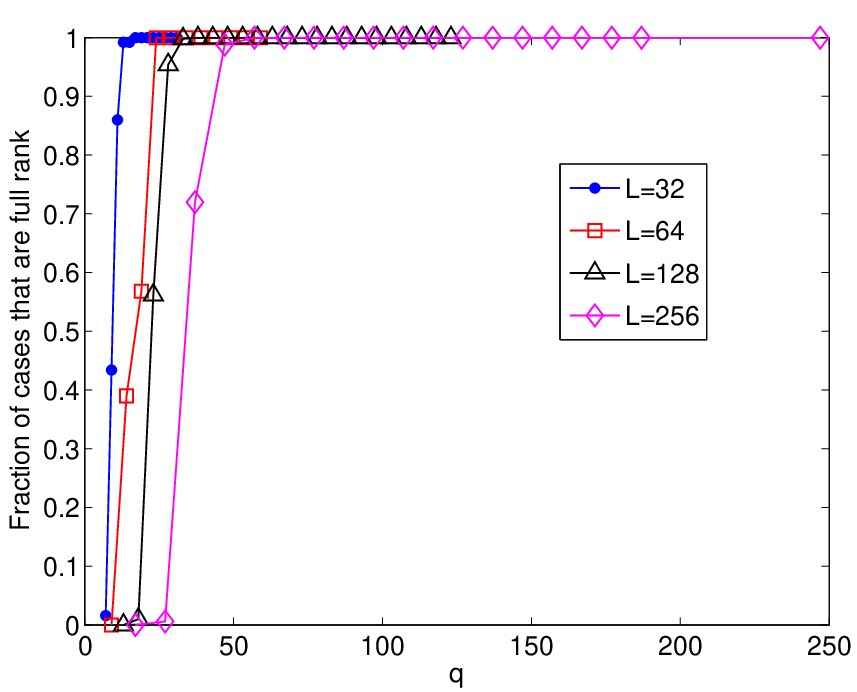
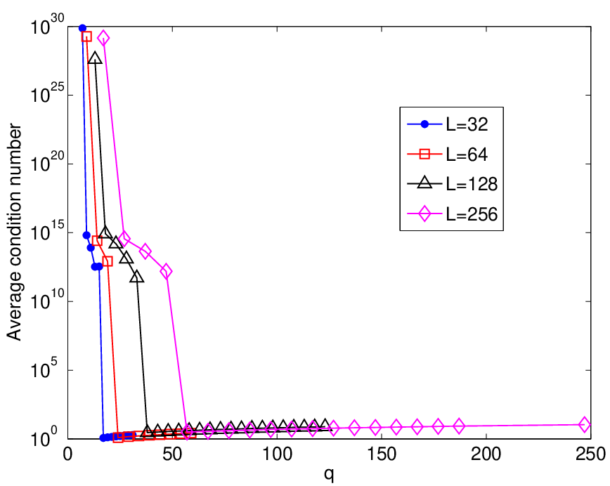
Fig. 3 offers empirical evidence suggesting that generating a sampling pattern uniformly at random from can be a simple and effective way of constructing a full rank , provided the ratio of its dimensions is small enough. The plots show the results from four trials corresponding to four different values of . For each trial, was fixed and was allowed to range from its minimum value—the smallest integer value satisying —to its maximum value . For each pair, 500 sampling patterns (of length ) were generated and the fraction of those that produced full rank are recorded in the left hand plot. The right hand plot displays the average condition number of in each case. Both plots suggest that after some threshold point random sampling patterns consistently produce well-conditioned and full rank matrices for the noncompressive problem. For the four cases shown, the threshold occurs when the ratio roughly equals 0.12, but a formal treatment of this phenomenon is beyond the scope of this paper.
For larger ratios (still falling within the noncompressive problem), full rank can sometimes be constructed by choosing the sampling pattern to be a Golomb ruler [32]. Golomb rulers are integer sets whose difference sets contain unique elements. The cardinality of the integer set is the ruler’s order and the largest difference between two integers is its length. The idea is that the integers represent marks on an imaginary ruler and the elements of the difference set are all the lengths that can be measured by the ruler. The goal in the study of Golomb rulers is to find the minimum length rulers for a given order. In the present context, however, we are only interested in using already tabulated rulers. For example, for and , one can take the minimum-length order-10 ruler to be the sampling pattern
Note that the ruler’s length, 55, is less than as it should be for MC sampling. This pattern yields a full rank with condition number whereas in Fig. 3 random patterns never produced a full rank matrix out of 500 test cases. The implication of this improvement is somewhat limited however because there are relatively few known (up to order 26) minimum length Golomb rulers. For instance with , the minimum value is 33, but there are no known minimum length Golomb rulers with orders greater than 26. When applicable, Golomb ruler sampling patterns can be an effective means to obtain a full rank when the ratio is near the threshold value. Note also that Ariananda et al. advocate the use of Golomb rulers in their study of multi-coset PSD estimation, but they used it to ensure the rank of a binary matrix [20].
3.3 Compressive solutions (underdetermined and sparse case)
When (28) is underdetermined and the sampling pattern is chosen uniformly at random from , is a randomly subsampled DFT matrix which is a well-known type of CS measurement matrix. Thus a number of CS recovery algorithms (e.g., [26, 27, 28]) will solve (28), provided is sparse and the number of CS measurements (length of ) is sufficient. However, because (28) has special structure, the usual CS recovery algorithms may be replaced by a non-negative least squares approach. This claim rests on the following result of Donoho and Tanner [33] (see also [34]):
Corollary 1 ([33], Corollary 1.4 and 1.5).
Assume is even and for , let be the partial DFT matrix ()
Let be a non-negative -sparse vector, i.e., let have at most nonzero positive entries. Then given the linear measurements , any approach that solves the linear system and maintains nonnegativity will correctly recover the -sparse solution , provided .
The corollary says that when is -sparse and non-negative, one needs only Fourier measurements to uniquely recover it. Moreover, the theorem states that can be recovered using any algorithm that produces a nonnegative solution to . The fact that a dimensional -sparse vector can be recovered from only Fourier measurments is an archetypical CS result. However, in contrast to typical CS recovery strategies, signal recovery in this case does not require explicit use of a sparsity constraint like minimization (see for example (12)). The reason is that this result is a specific case of a more general phenomenon in the recovery of sparse nonnegative vectors for underdetermined linear system of equations. In essence, it is known that if the row span of a measurement matrix intersects the positive orthant and if the vector to be recovered is nonnegative then the solution to the underdetermined linear system is a singleton, provided the vector of interest is sparse enough [35, 36] (see also [37]). This finding is key since it implies that compressive PSD estimates can be obtained in a manner similar to noncompressive estimates, i.e., they can be obtained using NNLS (more about this point in a moment).
The application of Corollary 1 to (28) is straightforward. The required matrix is a permuted version of provided the sampling pattern is chosen such that the set of differences form the consecutive sequence . In particular, can be constructed from as
| (30) |
The value for is chosen such that , i.e., such that the number of measurements (length of ) is greater than twice the sparsity.
One strategy to construct a sampling pattern that forms the difference set is to again use Golomb rulers. Most Golomb rulers do not produce a difference set that is a consequence sequence up to its length, but because differences do not repeat for Golomb rulers, they tend to furnish nearly consecutive sequences. For example, the order-7 minimum length ruler produces the difference set:
| (31) |
which nearly forms the consecutive sequence , missing only the elements . In Section 4.2, we present an example that uses this sampling pattern to successfully recover a 16-sparse vector . If an appropriate Golomb ruler (sampling pattern) does not exist for a given and , one can use other CS recovery approaches (e.g., minimization, CoSaMP [27], or iterative hard thesholding [28]) with a randomly generated sampling pattern.
The non-negativity requirement of Corollary 1 for is met asymptotically as . This claim can be inferred from Section 3 where it is shown that the entries of approach integrated periodogram estimates, which are non-negative by construction (see (22) through (25)). For PSD estimation, the non-negativity requirement is natural since by definition power spectra are non-negative.
When Corollary 1 can be applied, we compute compressive estimates using NNLS:
| (32) |
which is an optimization problem that can be solved via a linear program. Choosing a NNLS approach for compressive estimates is advantageous because noncompressive estimates can also be computed using a NNLS algorithm (and is perhaps preferred since can be negative; see Fig. 8).
3.4 Tradeoffs in noncompressive case
Given a sampling pattern that produces a full column rank , the relation establishes a tradeoff between and (Fig. 4) and tradeoffs among other related quantities (Fig. 5). For example, it establishes a tradeoff between system complexity and the estimate’s resolution, where here system complexity is simply taken to be the number of channels . As the left hand plot in Fig. 5 shows, finer resolution (smaller ) comes at the price of higher system complexity. As a concrete example, consider a WSS signal band-limited to 1 GHz and a desired resolution of 5 MHz, implying . A noncompressive solution would then require at least 21 channels; however, if a resolution of 15 MHz suffices, the number of channels could be reduced to 13 (see Fig. 5).
If one has the the freedom to choose and , the ratio can be driven to zero even while maintaining the inequality . This means that noncompressive estimates can theoretically be computed at arbitrarily low sampling rates and at finer and finer resolutions (see right hand plot of Fig. 5). Estimation at arbitrarily low sampling rates is a property shared with exisiting alias-free PSD estimators [38, 39, 40, 41, 42] that are based on random sampling where the set of sampling instances are (typically) realizations of a stochastic point process (e.g., a Poisson point process). Arbitrarily low sampling rates and arbitrarily fine resolutions, however, require arbitrarily high numbers of channels and arbitrarily long signal acquisition times. Thus in practical noncompresive situations, an appropriate balance needs to be struck between and that satisfies the requirements of a given application. Section 4.1 provides evidence of this tradeoff in a specific example.


3.5 Improved tradeoffs in compressive case
With sufficient sparsity, (28) can be uniquely solved even if it is underdetermined, i.e., even if [1, 3, 4]. This means that compressive estimates can be computed with better tradeoffs compared to noncompressive ones, i.e., for a given , a compressive estimate can be recovered with a smaller than what is possible for a noncompressive estimate, or conversely, for a given , a compressive estimate can be recovered with a larger .
The degree of the gain depends on the level of sparsity of at a specific resolution . Let denote the sparsity (number of nonzero elements) of at resolution . Then according to Corollary 1, a compressive estimate can be computed with or more Fourier measurements. Because the number of measurements in (28) equals (length of ), the need for measurements sets a minimum . Since compressive estimates pertain to underdetermined linear systems, the condition sets a maximum . To apply Corollary 1, however, a sampling pattern of length must exist that produces the set of differences . If sampling pattern does not exist for the minimum value, larger values must be considered. Thus, for a compressive estimate, the value of depends on the sparsity of (for a given ) and on the availability ability of an appropriate sampling pattern. We discuss specific examples in the next paragraph. Note that if an alternative CS recovery algorithm is used to solve (28) instead of applying Corollary 1, larger values will be needed for a given (and ) because these algorithms required larger numbers of measurements.
We illustrate the improved tradeoffs in two scenarios each of which are based on the presumption that is a 16-sparse vector at resolution (). The results are graphically shown in Fig. 4. As described above, the light shaded regions represent the pairs for which noncompressive estimates can be computed44 4 Again, the ability to compute a noncompressive estimate for a valid pair also depends on whether a suitable sampling pattern can be found., and are bordered by the curve . The darked shaded regions in each panel represent the pairs for which compressive estimates can be computed. The difference between the compressive regions on the left and right plots is that the region on the left presumes changes with and the one on the right presumes is independent of , i.e., it remains constant as varies. In the left hand plot, we assume doubles every time doubles. Thus, in comparison to the initial presumption at , we assume at which implies a mimimum . This behavior models the situation where the active subbands of at resolution contain energy at every frequency within the subband, so as the subbands are subdivided, increases. The scenario on the right reflects the situation where the active subbands only contain energy at one specific frequency, so remains constant as increases.
To judge the implications of these tradeoffs, we examine the associated tradeoffs among system complexity (), resolution (), and average system sampling rate () in Fig. 5. As above, the compressive regions are drawn under the presumption that for . The plots, however, are only for the case where is independent of . Intuitively, this represents a best case scenario in terms of “CS gain” over the noncompressive case (best possible improvements in for a fixed and in for a fixed ). The left hand panel shows system complexity as a function of resolution where GHz. The right hand panel plots resolution versus system sampling rate. The plots show that for this particular scenario, a CS approach can have appreciable benefits when the underlying PSD is sparse. For example, in Section 3.4 we stated that the recovery of with a resolution of 15 MHz required a 13 channel MC sampler for a noncompressive estimator. However, for a 16-sparse vector , a compressive estimate with the same resolution can be recovered with only channels, a reduction of almost 1/2. This gain is depicted in Fig. 5 as the shift from point (2) to point (3). The same reduction factor can also be seen in average system sampling rate (right hand plot of Fig. 5).
These improved tradeoffs may or may not effect the error in the recovered estimate. If is held fixed and is sparse, then as described above, can be reduced to the smallest integer such that (according to Corollary 1). This reduction in reduces the overall system sampling rate; however, the error in the recovered compressive estimate is not significantly different from the error in a corresponding noncompressive estimate because CS theory guarantees accurate (if not exact) recovery of . Now, if is held fixed and is increased, the sampling rate of each channel decreases. Thus, if the observation interval is fixed, the correlation estimates become worse (in the sense that their error is larger) because less and less samples are used to compute . In this case, CS still allows the recovery of an estimate, but its quality is declining as increases. To maintain accuracy, one must increase the observation interval and collect more samples per channel.
3.6 Consistency of the noncompressive estimator
To simplify notation, we examine the bias and variance of the least squares solution to instead of the solution of the expanded version . The analysis is equivalent in either case. Assuming is full rank, the noncompressive solution is
where denotes Hermitian transpose and is shorthand notation for the pseudoinverse.
Bias. The bias of is the amount its expected value differs from . Taking the expectation, we have . One element of equals
| (33) | ||||
| (34) | ||||
| (35) | ||||
where, as in (27), is an index for the pair , the second equality follows from (16) and (17), and is a discrete rectangular window
It is straightforward to show that
| (36) |
By substituting this expression back into (35), it is clear that is a biased estimate for finite ; however asympotically, is unbiased since
| (37) | ||||
| (38) | ||||
| (39) |
implies as .
Variance. The covariance matrix of is
| (40) |
where is the covariance matrix of . The diagonal elements of (40) are the variances of the elements of :
| (41) |
where . Note that in (41) we have dropped the subscript in our notation for the elements of . To show that as , we proceed to upper bound (41) with a sequence in that approaches zero as .
First, we note that the inequality [43, p. 336] implies
| (42) |
Second, for the correlation estimate it is well-known [30, p. 320] that55 5 The reason for the approximation in (43) is that this expression is derived assuming that and are jointly Gaussian; however, the result applies to other distributions as well [30].
| (43) |
Hence, if is square-summable, approaches zero as . Bound (41) by
| (44) |
Then from (42) and (43), we conclude that , and thus , approach zero as .
The noncompressive estimator is thus statistically consistent since it is asymptotically unbiased and since its variance decreases to zero as . Incidentally, if is a zero-mean Gaussian WSS random process, is also asymptotically efficient [43, p. 471], meaning that the variance of the limit distribution of achieves the Cramér-Rao bound. As we show in the Appendix, asymptotic efficiency follows from the fact that is a maximum likelihood estimate of .
3.7 Consistency of the compressive estimator
A detailed analysis of the compressive estimator’s consistency is beyond the scope of this paper because it depends on the specific CS recovery algorithm is employed. Nevertheless, compressive estimates are consistent in the sense that ideally sparse vectors can be exactly recovered by some CS recovery algorithms, and thus the consistency of (as shown above) implies the consistency of .
4 Examples
4.1 Estimating MA spectra with lines
Consider sampling a (nonsparse) moving average power spectrum with spectral lines using a 50 channel MC sampler (). The process is generated by passing white noise (with unit variance) through a filter with transfer function and then adding the two sinusoidal components, and . Fig. 6(a) shows the true PSD. Fig. 6(b) and Fig. 6(c) show two resulting noncompressive estimates for different values of , the number of MC samples per channel. For comparison, a coarse resolution approximation of the true PSD is overlaid on the estimates. Because is consistent, its mean squared error with respect to this coarse resolution approximation decreases to zero as . This is depicted in Fig. 6(c). Fig. 7 further illustrates the consistency of within the context of this example for various values. In each case, the average squared error monotonically decreases as increases.


4.2 Sparse multiband power spectra
Suppose a real WSS random process has a sparse multiband power spectrum band-limited to GHz ( GHz). Suppose also that we are interested in a PSD estimate having a resolution of about 15 MHz. To satisfy this requirement we choose which gives a resolution of 15.625 MHz. Suppose also that the sparse PSD is composed of two active bands, each with an approximate bandwidth of 30 MHz. Being conservative, we thus expect to be a 16-sparse vector (including positive and negative frequencies with each active band taking up 4 adjacent subbands).


The PSD can be estimated in either a noncompressive or a compressive manner. Choosing , leads to an overdetermined system in (21) () and a noncompressive estimate. Fig. 8(a) shows the resulting noncompressive estimate with a normalized square error of . The error is calculated with respect to a coarse Welch estimate, i.e., it has the same resolution as the noncompressive estimate. The Welch estimate is based on uniform Nyquist rate samples and is computed with no overlap. The sampling pattern was chosen uniformly at random from the set and it was verified that had full rank. The fractional delays were implemented by interpolating the MC sequences to the Nyquist rate, shifting them by the appropriate delays, and then subsampling them to the original rate. Each channel collected 1000 MC samples and the average system sampling rate was about 1/6 of the Nyquist rate.
According to Corollary 1, the number of measurements required to recover a 16-sparse vector needs to be greater than or equal to 32. This implies that needs to be at least 7 because the number of measurements in (28) equals and for this quantity is less than 32. In addition, Corollary 1 requires that the sampling pattern produces the set of differences for a 16-sparse signal. Fortunately, a Golomb ruler of order 7 () exists that produces the necessary difference set. Fig. 8(b) shows the resultant compressive estimate (normalized squared error ). The reduction in the number of channels from 13 to 7, in going from the noncompressive to the compressive estimator, reduces the complexity of the sampler, or equivalently, halves the average system sampling rate.
Fig. 8(c) displays the same compressive estimate as in Fig. 8(b) except that it is computed with 10000 samples per channel instead of 1000. The normalized squared error is . In contrast to this figure, Fig. 8(d) shows the minimum () norm least squares solution computed by the pseudoinverse. As one would expect, this solution is far from the true PSD and does not improve with more samples.
4.3 Spectral sensing for cognitive radio
To opportunistically use their resources, cognitive radios must be able to dynamically sense underutilized portions of the radio spectrum. Towards this end, methods and algorithms have recently been proposed to sense the largest possible bandwidth while sampling at the lowest possible rate [19]. Some of these methods have taken advantage of CS, but the following example shows that a noncompressive estimator can monitor large bandwidths at low sampling rates (although, as explained above, CS will allow better tradeoffs with a compressive estimator).
This example is only a caricature of the actual problem that must be solved to realize a practical cognitive radio system. Let be a MA random process generated from filtering white Gaussian noise with a notch filter. The filter notches the spectrum such that it has approximately two MHz stop bands within an overall band of GHz ( GHz). Fig. 9 shows two noncompressive estimates and compares them to a Welch estimate of the same resolution and calculated using Nyquist samples. The left plot sets and and the right plot sets and , meaning that the resolution of left hand estimate is half the resolution of the right hand estimate (half as fine) and that the sampling rate per channel on the left is twice that of the right (31.25 MHz vs 15.625 MHz) In each case, however, the overall average system sampling rate is the same (781.25 MHz). The noncompressive estimate on the left is formed with 4096 MC samples per channel, the one on the right with 2096 samples. Both plots suggest that spectral holes could be detected simply by thresholding the estimates and hence noncompressive estimators may provide a way to monitor large bandwidths at low sampling rates.


5 Conclusion
In this paper, we derived and analyzed a consistent, MC based PSD estimator that produces both compressive and noncompressive estimates at sub-Nyquist sampling rates. The estimator does not estimate the power spectrum on a discrete grid of frequencies but instead computes average power within a given set of subbands. Compressive estimates leverage the sparsity of the spectrum and exhibit better tradeoffs among the estimator’s resolution, complexity, and average sampling rate compared to noncompressive estimates. Given suitable sampling patterns, both compressive and noncompressive estimates can be recovered using NNLS, thus avoiding the overhead of computing the estimates in different ways. The estimator is consistent and has wide applicability; it is especially attractive in wideband applications where high sampling rates are costly or difficult to implement.
6 Appendix
To show that is asymptotically efficient, we show that it is a maximum likelihood estimator (MLE) because MLEs are known to be asymptotically efficient [43, p. 472].
Define to be the th snapshot of samples across all the channels of a MC sampler:
| (45) |
The entries of are the nonuniform samples collected within one period ( seconds) of the MC sampling sequence. The upper triangular portion of the sample correlation matrix are the elements of :
| (46) | ||||
| (47) |
Suppose is zero-mean WSS Gaussian random process. Then each snapshot is an i.i.d. realization of a jointly Gaussian random vector with correlation matrix . Taking to be the parameter of interest, the log-likelihood function given the data is [44, 45]
| (48) |
The maximum likelihood estimate of can be found by taking the gradient of with respect to and setting the result equal to zero.
| (49) |
Solving for reveals that the maximum likelihood estimate of equals the sample correlation , or in other words, the entries in are maximum likelihood estimates of for all combinations of pairs .
References
- [1] E. Candes, J. Romberg, and T. Tao, “Robust uncertainty principles: Exact signal reconstruction from highly incomplete frequency information,” IEEE Trans. Info. Th., vol. 52, no. 2, pp. 489–509, Feb. 2006.
- [2] E. Candes and T. Tao, “Near-optimal signal recovery from random projections:Universal encoding strategies?,” IEEE Trans. Info. Th., vol. 52, no. 12, pp. 5406–5425, Dec. 2006.
- [3] D. Donoho, “Compressed sensing,” IEEE Trans. Info. Th., vol. 52, no. 4, pp. 1289–1306, Apr 2006.
- [4] E.J. Candes and M.B. Wakin, “An introduction to compressive sampling,” IEEE Signal Processing Mag., vol. 25, no. 2, pp. 21–30, Mar 2008.
- [5] J. Romberg, “Compressive sensing by random convolution,” SIAM J. Imaging Sci., vol. 2, no. 4, pp. 1098–1128, 2009.
- [6] J. Tropp, J. Laska, M. Duarte, J. Romberg, and R. Baraniuk, “Beyond Nyquist: Efficient sampling of sparse bandlimited signals,” IEEE Trans. Info. Th., vol. 56, no. 1, pp. 520–544, 2010.
- [7] M. Mishali and Y.C. Eldar, “From theory to practice: Sub-Nyquist sampling of sparse wideband analog signals,” IEEE J. Sel. Topics Sig. Process., vol. 4, no. 2, pp. 375 –391, 2010.
- [8] M. A. Lexa, M. E. Davies, and J. S. Thompson, “Reconciling compressive sampling systems for spectrally sparse continuous-time signals,” Signal Processing, IEEE Transactions on, vol. 60, no. 1, pp. 155 –171, Jan. 2012.
- [9] P. Feng and Y. Bresler, “Spectrum-blind minimum-rate sampling and reconstruction of multiband signals,” Proc. IEEE Inter. Conf. on Acoustics, Speech, and Signal Processing, vol. 3, pp. 1688–1691, May 1996.
- [10] Ping Feng, Universal Minimum-Rate Sampling and Spectrum-Blind Reconstruction for Multiband Signals, Ph.D., University of Illinois at Urbana-Champaign, 1997.
- [11] R. Venkataramani and Y. Bresler, “Perfect reconstruction formulas and bounds on aliasing error in sub-Nyquist nonuniform sampling of multiband signals,” IEEE Trans. Info. Th., vol. 46, no. 6, pp. 2173–2183, Sep 2000.
- [12] Y. Bresler, “Spectrum-blind sampling and compressive sensing for continuous-index signals,” IEEE Info. Th. and Appl. Workshop, pp. 547–554, Jan 2008.
- [13] M. Mishali and Y. Eldar, “Blind multiband signal reconstruction: Compressed sensing for analog signals,” IEEE Trans. Signal Processing, vol. 57, no. 3, pp. 993–1009, 2009.
- [14] Cormac Herley and Ping Wah Wong, “Minimum rate sampling and reconstruction of signals with arbitrary frequency support,” IEEE Trans. Info. Th., vol. 45, no. 5, pp. 1555–1564, Jul. 1999.
- [15] P.P. Vaidyanathan and Vincent C. Liu, “Efficient reconstruction of band-limited sequences from nonuniformly decimated versions by use of polyphase filter banks,” IEEE Trans. Acoust., Speech and Signal Processing, vol. 38, no. 11, pp. 1927–1936, Nov. 1990.
- [16] M.A. Lexa, M.E. Davies, and J.S. Thompson, “Compressive spectral estimation can lead to improved resolution/complexity tradeoffs,” in 4th Workshop on Signal Processing with Adaptive Sparse Structured Representations, Jun 2011, p. 72.
- [17] Z. Tian and G.B. Giannakis, “Compressed sensing for wideband cognitive radios,” in Proc. IEEE Inter. Conf. on Acoustics, Speech, and Signal Processing, 2007, vol. 4, pp. 1357–1360.
- [18] Geert Leus and Dyonisius Dony Ariananda, “Power spectrum blind sampling,” IEEE Signal Processing Letters, pp. 443–450, Aug. 2011.
- [19] Dyonisius Dony Ariananda and Geert Leus, “Wideband power spectrum sensing using sub-Nyquist sampling,” in Proc. IEEE Inter. Workshop on Sig. Processing Advances in Wireless Comm., Jun 2011.
- [20] D.D. Ariananda, G. Leus, and Z. Tian, “Multi-coset sampling for power spectrum blind sensing,” in Digital Signal Processing (DSP), 2011 17th International Conference on, Jul. 2011, pp. 1 –8.
- [21] Petre Stoica, Prabhu Babu, and Jian Li, “New method of sparse parameter estimation in separable models and its use for spectral analysis of irregularly sampled data,” IEEE Trans. Signal Processing, vol. 59, no. 1, pp. 35–47, 2011.
- [22] Petre Stoica, Prabhu Babu, and Jian Li, “SPICE: A sparse covariance-based estimation method for array processing,” IEEE Trans. Signal Processing, vol. 59, no. 2, pp. 629–638, 2011.
- [23] A. Papoulis, Probability, Random Variables, and Stochastic Processes, McGraw Hill, New York, 3 edition, 1991.
- [24] Richard Roberts and Clifford Mullis, Digital Signal Processing, Addison-Wesley Publishing Co., Inc., 1987.
- [25] T.I. Laakso, V. Valimaki, M. Karjalainen, and U.K. Laine, “Splitting the unit delay: Tools for fractional delay filter design,” IEEE Signal Processing Mag., vol. 13, no. 1, pp. 30–60, Jan 1996.
- [26] E. Cande’s, J. Romberg, and T. Tao, “Stable signal recovery from incomplete and inaccurate measurements,” Commun. Pure Appl. Math., vol. 59, no. 8, pp. 1207–1223, 2006.
- [27] D. Needell and J. Tropp, “COSAMP: Iterative signal recovery from incomplete and inaccurate samples,” Appl. Computational Harm. Anal., vol. 26, pp. 301–321, 2008.
- [28] T. Blumensath and M. Davies, “Interative hard thresholding for compressed sensing,” Appl. Comput. Harmon. Anal., vol. 27, no. 3, pp. 265–274, 2009.
- [29] Mark Rudelson and Roman Vershynin, “On sparse reconstruction from Fourier and Gausssian measurments,” Communications on Pure and Applied Mathematices, vol. 61, no. 8, pp. 1025–1045, Aug. 2008.
- [30] D.H. Johnson and D.E. Dudgeon, Array Signal Processing: Concepts and Techniques, Prentice Hall, Upper Saddle River, NJ, 1993.
- [31] Athanasios Papoulis, The Fourier Integral and Its Applications, McGraw-Hill, Inc., 1962.
- [32] Konstantinos Drakakis, “A review of the available construction methods for Golomb rulers,” Advances in Mathematics of Communications, vol. 3, no. 3, pp. 235–250, Aug. 2009.
- [33] David L. Donoho and Jared Tanner, “Counting the faces of randomly-projected hypercubes and orthants, with applications,” Discrete and Computational Geometry, vol. 43, no. 3, pp. 522–541, 2010.
- [34] David L. Donoho and Jared Tanner, “Counting the faces of randomly-projected hypercubes and orthants, with applications,” [Online] arXiv:0807.3590v1 [math.MG], 2008.
- [35] A.M. Bruckstein, M. Elad, and M. Zibulevsky, “On the uniqueness of nonnegative sparse solutions to underdetermined systems of equations,” IEEE Trans. Info. Th., vol. 54, no. 11, pp. 4813–4820, 2008.
- [36] Martin Slawski and Matthias Hein, “Robust sparse recovery with non-negativity constraints,” in 4th Workshop on Signal Processing with Adaptive Sparse Structured Representations, Jun 2011, p. 30.
- [37] David L. Donoho and Jared Tanner, “Sparse nonnegative solution of underdetermined linear equations by linear programming,” Proc. Nat. Acad. Sci. USA, vol. 102, no. 27, pp. 9446–9451, 2005.
- [38] Bashar I. Ahmad and Andrzej Tarczynski, “Reliable wideband multichannel spectrum sensing using randomized sampling schemes,” Signal Processing, vol. 90, pp. 2232–2242, 2010.
- [39] Andrzej Tarczynski and Dongdong Qu, “Optimal random sampling for spectrum estimation in DASP applications,” Int. J. Appl. Math. Comput. Sci., vol. 15, no. 4, pp. 463–469, 2005.
- [40] E. Masry, “Poisson sampling and spectral estimation of continuous-time processes,” IEEE Trans. Info. Th., vol. 24, no. 2, pp. 173 – 183, Mar 1978.
- [41] E. Masry, “Alias-free sampling: An alternative conceptualization and its applications,” IEEE Trans. Info. Th., vol. 24, no. 3, pp. 317–324, May 1978.
- [42] F. Beutler, “Alias-free randomly timed sampling of stochastic processes,” Information Theory, IEEE Transactions on, vol. 16, no. 2, pp. 147 – 152, Mar 1970.
- [43] George Casella and Roger L. Berger, Statistical Inference, Duxbury, 2002.
- [44] C.T. Mullis and Louis L. Scharf, Modern Spectral Estimation, chapter Quadratic Estimators of the Power Spectrum, pp. 1–57, Houghton-Mifflin, 1990.
- [45] L.L. Scharf, Statistical Signal Processing: Detection, Estimation, and Time Series Analysis, Addison-Wesley Publishing Co., Reading, MA, 1991.