The model in polar coordinates at nonzero temperature
Abstract
We study the restoration of spontaneously broken symmetry at nonzero temperature in the framework of the model using polar coordinates. We apply the CJT formalism to calculate the masses and the condensate in the double-bubble approximation, both with and without a term that explicitly breaks the symmetry. We find that, in the case with explicitly broken symmetry, the mass of the angular degree of freedom becomes tachyonic above a temperature of about MeV. Taking the term that explicitly breaks the symmetry to be infinitesimally small, we find that the Goldstone theorem is respected below the critical temperature. However, this limit cannot be performed for temperatures above the phase transition. We find that, no matter whether we break the symmetry explicitly or not, there is no region of temperature in which the radial and the angular degree of freedom become degenerate in mass. These results hold also when the mass of the radial mode is sent to infinity.
pacs
11.10.Wx,12.39.Fe,11.30.RdMUSO Collaboration
CLEO Collaboration
I Introduction
The model is of great importance for the theory of critical phenomena [1] and has been intensely studied in different theoretical frameworks [2, 3, 4, 5, 6, 7, 8, 9]. Using a mass term with a ‘wrong’ sign, the symmetry is spontaneously broken to in the vacuum. At sufficiently high temperature , the symmetry is restored. The case has been profusely investigated because of its application to the chiral phase transition in quantum chromodynamics (QCD) [10, 11, 12, 13, 14, 15]. QCD has a chiral symmetry (where is the number of quark flavors) which is spontaneously broken to in the vacuum. The group is locally isomorphic to , and is locally isomorphic to . Therefore, using the universality hypothesis, the model can be considered as an effective theory for the restoration of chiral symmetry in QCD with two quark flavors.
Most studies of symmetry restoration within the model [10, 11, 12, 14, 15] have been performed in Cartesian coordinates, . Then, when the symmetry is spontaneously broken, the first coordinate is usually selected to assume a non-vanishing vacuum expectation value , , and the remaining coordinates are taken to be the Goldstone modes arising from spontaneous symmetry breaking. However, in the absence of explicit symmetry-breaking terms, the effective potential is of the well-known ‘Mexican hat’-type, with any state on the circle being energetically degenerate with the vacuum state . Therefore, the Goldstone modes actually correspond to angular variables when moving along the circle , and the massive degree of freedom corresponds to the radial degree of freedom when trying to ‘climb’ the rim of the hat.
This observation constitutes the main motivation for the present paper where we study symmetry restoration within the model in polar coordinates. For the sake of simplicity, we shall concentrate on the case , because the transition from Cartesian to polar coordinates is particularly simple in this case. Nevertheless, the conceptual issues are the same in this case as for . In a certain sense, the case corresponds to QCD with one flavor in the absence of the axial anomaly. For , the (most simple) anomaly term would introduce a linear term in the massive degree of freedom, corresponding to an explicit symmetry breaking term. This is different from the two-flavor case, i.e., , which corresponds to the case of maximal anomaly or maximal breaking. Due to the similarities with the chiral symmetry of QCD and its breaking and restoration at nonzero , in the following we shall also refer to the transition in the model as ‘chiral transition’. The order parameter for the transition, , will be called ‘chiral condensate’, and the two degrees of freedom (the ‘chiral partners’) are referred to as the meson and the pion. The so-called ‘chiral limit’ is the case where explicit symmetry-breaking terms are sent to zero, in which case the pion becomes a true Goldstone boson.
Another motivation for our work is that, if we send the mass of the radial degree of freedom (the meson) to infinity, we just obtain the leading-order Lagrangian of chiral perturbation theory () [16, 17, 18], with the Goldstone boson (the pion) as angular degree of freedom. In our simplified framework of the model, it is then possible to perform a test of the validity of angular variables at nonzero .
The transition from Cartesian to polar coordinates represents a change of the representation of the same theory. Obviously, physical quantities should be independent from the adopted representation. This fact is ensured by the so-called -matrix equivalence theorem [19] which states that the elements of the -matrix do not change when performing a transformation of the fields. However, for actual calculations one must use a certain approximation scheme. Then, the results obtained in one representation are not necessarily equal to those obtained in another representation [20]. In this work we shall explicitly show that, by using the CJT formalism in the double-bubble approximation [21], quantities computed in polar coordinates are actually quite different from those evaluated in the standard Cartesian coordinates.
Our results are the following: (i) for explicit symmetry breaking, the pion mass becomes tachyonic at high , signalizing a breakdown of the CJT formalism in the double-bubble approximation. (ii) When the explicit symmetry-breaking term is sent to zero (which, in analogy to the case , we refer to as the chiral limit), the Goldstone boson (pion) remains massless at each in polar coordinates, thus satisfying the Goldstone theorem. This is contrary to Cartesian coordinates where a nonzero value of the pion mass is obtained as soon as the temperature is switched on, see e.g. Ref. [12]. However, due to singular terms in the equations for the masses and the condensate, and because the order parameter above the phase transition, the model becomes ill-defined. (iii) Both with and without explicit symmetry breaking, there is no region of temperature in which the chiral partners become degenerate in mass. (iv) Similar results hold also in the nonlinear limit, i.e., when the radial excitation becomes infinitely heavy.
The reason why polar coordinates are problematic at high can be traced back to the decreasing value of the chiral condensate : in fact, in polar coordinates there are interaction terms proportional to inverse powers of , which render the application of the CJT formalism (or any other resummation scheme) problematic when is too small. In order to circumvent this problem one can perform a slightly different transformation to polar coordinates, in which the polar coordinates are not defined with respect to the origin of the Cartesian coordinates [22]. In this way a smooth limit from Cartesian to polar coordinates is realized, in which all the results of Cartesian coordinates can be reobtained. Interestingly, it is possible to investigate these issues also in the very simple situation of a free Lagrangian, see Sec. IV for details. In the Cartesian representation the results for thermodynamical quantities, such as the pressure, are exact in this case. The deviations of the results in the polar representation from the Cartesian one explicitly show the limitations of polar coordinates.
A further issue of polar coordinates is the fact that the Jacobian associated with the field transformation is not unity: an additional term emerges in the transformation of the interaction measure, which is potentially relevant in the context of quantum field theory. We discuss in detail why it is justified to neglect its contribution for our conclusions. For this purpose, we rely on perturbative cancellations between Jacobian contributions and certain divergences (which will be shown in detail in Appendix C), we discuss the vanishing of the Jacobian contributions in the dimensional regularization scheme, and we study a different field representation in terms of polar variables, in which the Jacobian is indeed unity. In all cases we studied, the qualitative picture does not change and the same conceptual issue of diverging interaction terms in the high-temperature region exists also in this case.
The paper is organized as follows: In Sec. II we write the model in terms of polar coordinates and discuss the subtleties concerning this coordinate transformation. In Sec. III we apply the CJT formalism and present the numerical results. The simple case of a free Lagrangian is discussed in Sec. IV. In Sec. V the alternative representation with unit Jacobian is discussed. Finally, we give our conclusions and an outlook in Sec. VI. Our units are ; the metric tensor is .
II The model in polar coordinates
II.1 Tree level, zero temperature
The model in Cartesian coordinates , including an explicit symmetry breaking term , is described by the Lagrangian
| (1) |
As usual, we consider the shift where is a constant. At zero temperature the minimization of the potential leads to the minimum satisfying the following equation:
| (2) |
When the symmetry of the Lagrangian (1) under transformations is exact. For and the global minimum is realized for , i.e., the ground state breaks the symmetry spontaneously. The vacuum expectation value is referred to as ‘chiral condensate’ in our model. In the vacuum, the numerical value for is chosen to be the pion decay constant, MeV. When an additional explicit breaking of chiral symmetry is realized.
By shifting the fields around their values at the global minimum, one obtains the zero-temperature tree-level masses and as
| (3) |
It is clear that for , i.e., this particle represents the Goldstone boson emerging from the spontaneous breaking of chiral symmetry.
We now introduce polar coordinates through the transformation
| (4) |
leading to
| (5) |
Just as above, one shifts the field as . At zero temperature the minimization of the potential leads to the same Eq. (2) for the minimum . Also the zero-temperature tree-level masses and coincide with the expressions of Eq. (3):
| (6) |
In order to extract , we have expanded the cosine in Eq. (5).
II.2 Mathematical issues using polar coordinates: The Jacobian and the integration intervals
Denoting and taking into account that the Jacobian of the transformation in Eq. (4) is , the partition function can be rewritten as
| (7) |
where periodic boundary conditions are understood: , etc. The suffix means that the Lagrangians are considered in Euclidean space.
The r.h.s. of Eq. (7) describes the partition function in polar coordinates. Due to the fact that the Jacobian is not unity and that both fields and do not vary between the question arises if we can apply the usual Feynman rules to the Lagrangian .
One can rewrite the contribution of the Jacobian as
| (8) |
where is an infinite constant of dimension energy4. (In discretized Euclidean space-time is the lattice spacing in time and the lattice spacing in spatial direction.) In the following, we also use the notations
| (9) |
It is evident that the term in the exponent of Eq. (8) induces a divergent contribution to the effective action requiring regularization. In the framework of dimensional regularization the contribution of the Jacobian vanishes in virtue of Veltman’s rule [23], see also the explicit perturbative analyses performed in Refs. [24, 22, 9]. Since the transformation to polar coordinates turns a renormalizable Lagrangian into a non-renormalizable one, one expects a perturbative cancellation of divergent contributions from the non-renormalizable term appearing in Eq. (5) with the divergent contributions from the Jacobian. Indeed, it was shown in Ref. [9] that divergent contributions, , arising from the momentum-dependent interaction term, exactly cancel the vertices from the Jacobian order by order in a perturbative loop expansion. Using a power-counting argument, we demonstrate explicitly in Appendix C how this cancellation works for the CJT effective potential. However, it turns out that the cancellation does not occur for a truncation of the CJT effective potential at a given loop order (e.g. in Hartree approximation where only double-bubble diagrams are included), but only when higher-order loop contributions are taken into account (see Appendix C). We nevertheless omit contributions , assuming that the aforementioned cancellation has happened before studying a particular truncation of the effective potential. Therefore, we neglect the Jacobian from the beginning, independent of the renormalization scheme, and simultaneously omit terms arising from the momentum-dependent vertices [in our study this only concerns the first term appearing in Eq. (71)].
Apart from this general argument why to omit the Jacobian, we explicitly verified that the relevant features of our results are the same independent of the renormalization scheme (trivial regularization, counter-term regularization, or dimensional regularization scheme). In addition, in Sec. V we introduce polar coordinates in a slightly modified manner which corresponds to a unit Jacobian. Again, our conclusions remain unchanged.
We now turn to the extension of the range of integration over the fields and . The possibility to extend the angular integration interval, , originates from the periodicity of the integrand. This point is subtle since it is in general not possible to split a path integral over the interval into the sum of two path integrals over the intervals and , respectively. For potentials of the form and for -periodic potentials (as in the present case) one can show that extending the range of integration simply yields a countably infinite overall constant which can be absorbed into a normalization constant [25]. The extension in the direction from to can be achieved with the help of a modified Heaviside step function defined in such a way that its contribution vanishes in dimensional regularization [25].
Besides the divergences which cancel order by order in perturbation theory, one encounters the standard UV divergences in loop integrals, see Appendix A. In many-body resummation schemes, the cancellation of these divergences is subtle and commonly requires additional counter terms compared to those encountered in perturbation theory [26]. Unfortunately, we were not able to identify these counter terms in the polar coordinate representation, but we shall assume that they exist and cancel the above mentioned standard divergences.
II.3 Shift of the potential
In this section we show how to circumvent the problems arising from the fact that polar coordinates are ill-defined at the origin. Inspired by Ref. [22], we first shift the potential along the -axis by an arbitrary amount . In this way the global minimum realized at the critical temperature (and above) is not located at , but at . After the shift, the Lagrangian (1) reads
| (10) |
When performing the transformation to polar coordinates, Eq. (4), we obtain
| (11) |
Note that obviously from Eq. (5), thus the study of Sec. II.1 can be regarded as a special case of this more general treatment. After performing a Taylor expansion of the trigonometric functions about and shifting , we can easily determine the additional tree-level contributions to the masses and the interaction vertices.
III Results at nonzero
In this section we present the results at nonzero temperature for the model described by the Lagrangian for different cases.
For reasons of simplicity, numerical results in Secs. III.1 – III.4 were obtained using the so-called trivial regularization: the vacuum part of the integrals is simply set to zero, for details see Appendix A. For a discussion of the alternative counter-term regularization and dimensional regularization schemes we refer to Sec. III.6.
III.1 ,
In this case the system is described by the Lagrangian (5) in Sec. II.1. The effective potential in the CJT formalism reads
| (12) |
where denotes the classical potential and the inverse tree-level propagators read
| (13) |
At nonzero the condensate and the masses become -dependent functions
| (14) |
and the dressed propagators are given by
| (15) |
where is a wave-function renormalization factor for the pion.
The term in Eq. (12) is the contribution of all 2PI vacuum graphs, denotes the connected 1-point function in the presence of a source, and denotes the full connected 2-point function in the presence of the source. In general, consists of infinitely many diagrams, which prohibits an explicit calculation of . In practice, one therefore has to restrict oneself to certain classes of diagrams. We shall use the so-called Hartree approximation where only double-bubble diagrams are taken into account:
By extremizing the effective potential in Eq. (12) we obtain the following equations:
| (16) | |||
| (17) | |||
| (18) | |||
| (19) |
where denotes, in general, an extremum. At the masses coincide with their tree-level values in Eq. (3) and . Furthermore,
| (20) |
| (21) |
| (22) |
The following numerical values are used at zero temperature: MeV, MeV, and MeV.

The numerical results for the masses, the condensate, and pressure can be found in the upper row of Fig. 1. The results for polar coordinates are also compared to the standard results obtained in Cartesian coordinates. One observes that in general the results in polar coordinates differ substantially from those in Cartesian coordinates, except for the pressure at low temperatures, where the agreement between solid and dashed curves is seen to be quite good. Moreover, although the condensate decreases sharply at a temperature MeV, indicating the onset of chiral symmetry restoration, the pion mass does not become degenerate with the mass for high . On the contrary, above a temperature MeV (where the curves in Fig. 1 terminate) it becomes tachyonic, signalizing a breakdown of the model for large . This fact shows a limitation of the application of angular variables at nonzero temperature, at least in the Hartree approximation.
The effective potential is shown in Fig. 2 for different temperatures. There is a region around the origin where the effective potential is not defined since no real-valued solutions exist. Due to the singular terms with inverse powers of there is no extremum at the origin. At low temperature there is only a global minimum at a large value . At a certain temperature a second minimum and a maximum (both at smaller values of ) occur. At MeV the effective potential assumes the same value at both minima, indicating a first-order phase transition. Above this temperature, the global minimum moves closer and closer to the origin, but never becomes zero. Above MeV no real solutions to the system of equations exist at the global minimum.
The reason why no real solution exists above is due to the fact that the pion mass becomes imaginary, and therefore the system is not stable. In order to see this in more detail, we show the function at in Fig. 3 (solid line). We observe that has an imaginary part below a value MeV. At the imaginary part vanishes and becomes a positive definite, real- (but multi-)valued function of . At , the value coincides with at the global minimum of the effective potential. The solid line above is the solution for which has to be used to plot the effective potential. Using the lower branch instead would lead to a discontinuous jump of the effective potential near MeV. Below the point is located such that the extremum , i.e., real solutions at the global minimum exist. With increasing temperature approaches and finally hits the ill-defined region for .


III.2 ,
In this section we study the case where the explicit symmetry breaking parameter is set to zero, . Equations (16)–(19) simplify to
| (23) | |||
| (24) |
Here, we have used Eq. (64) from Appendix A and the fact that to eliminate the pion tadpole term in Eq. (18). The numerical results for the masses, the condensate, and the pressure as functions of temperature are shown in the lower row of Fig. 1. Note that indicates that the Goldstone theorem is fulfilled at each below the chiral phase transition. This is a property which does not hold in Cartesian coordinates, see for instance the lower left panel of Fig. 1. Unfortunately, also above the transition, indicating that the chiral partners do not become degenerate in the chirally restored phase where .
The effective potential (relative to its value at its global minimum) for different temperatures is shown in Fig. 4. For temperatures in the transition region, one clearly observes the features of a first-order phase transition, i.e., three minima separated by two maxima.

III.3 ,
The chiral limit, i.e., , does not exist, since for arbitrarily small, but nonzero values of , the effective potential has no extremum near the origin . We have confirmed this numerically by taking successively smaller values of (compare discussion of Fig. 6). The reason for this non-analyticity of the chiral limit are the inverse powers of in Eqs. (16)–(19). When setting from the beginning, this problem does not exist because the singular terms are eliminated right away. Therefore, we conclude that the model cannot describe the chirally restored phase and is limited to the chirally broken phase. Again, polar coordinates have demonstrated a limited range of applicability. Interestingly, this problem does not exist in Cartesian coordinates where taking the limit is not problematic in the chirally restored phase.
III.4 ,
As argued in Refs. [22, 9], the non-analyticity at the origin encountered in the previous subsections can be eliminated by introducing a non-vanishing value for the parameter , i.e., shifting the vacuum expectation value to nonzero values . Now we have to consider the full Lagrangian (11). In the double-bubble approximation, the following equations are obtained:
| (25) |
| (26) |
| (27) |
| (28) |
In the limit the system of Eqs. (25)–(28) reduces to the system of equations for Cartesian coordinates [see Eqs. (28a,b), (30a) in Ref. [12] for with the replacement ]. This is easily explained by the fact that the radial as well as the angular variable are defined relative to the origin so that for large we have and . Hence, in the limit polar coordinates become Cartesian:
Solving the system of Eqs. (25)–(28) in the case yields the condensate shown in the middle panel of the upper row of Fig. 1 (dotted and dash-dotted lines). For values (for instance , dotted line) the manner in which the condensate is multi-valued reminds of the behavior for a first-order phase transition. However, for this to be the case, there would have to be a third solution for near the origin. This solution does not exist and therefore there is neither a first-order transition nor a restored phase. Above (dash-dotted line) the behavior of smoothly approaches the known Cartesian behavior, as expected.
III.5 The limit
In this section we study the properties of the nonlinear sigma model [27] in polar coordinates at nonzero temperature. This investigation is also interesting in comparison to chiral perturbation theory at nonzero temperature, see also Ref. [28] and refs. therein.
The nonlinear sigma model is obtained by taking the limit and keeping the ratio fixed. Inserting Eqs. (21) and (22) into Eq. (17) we obtain
| (29) |
For , the last term dominates. Therefore, if this term is positive definite, also . We have to demand that the last term is positive definite in order to have real-valued solutions for . Since for , the positive-definiteness of the last term requires that
| (30) |
This means that the range cannot be described, neither for nor for (i.e., ). Thus, the model is not applicable in the chirally restored phase where we expect . This result shows that it is not possible to describe the phase transition in polar coordinates (in the framework of the CJT formalism) when taking the limit to the nonlinear sigma model.
III.6 Dependence on the regularization procedure
It is important to verify how the results change when a different regularization scheme is employed. In this section we compare three different regularization schemes: the trivial regularization scheme, the counter-term regularization scheme of Ref. [12], and the dimensional regularization scheme of Ref. [29]. In the latter two cases we assume that suitable counter terms exist for the Hartree approximation in polar coordinates, see remark at the end of Sec. II.2.
In the counter-term scheme, the vacuum contribution of the thermal tadpole integral (60),
| (31) |
is not neglected as in the trivial regularization scheme but is first rewritten using the residue theorem,
| (32) |
This integral is then regularized by introducing a renormalization scale [12]:
| (33) |
We set for the counter-term scheme and for the dimensional regularization scheme, in order to satisfy the constraint for the vacuum value of the pion wave-function renormalization factor. The initial values , and correspond to the following parameter choice:
| (34) | |||
| (35) | |||
| (36) |
where from Eq. (33) for the counter-term scheme, and from Eq. (74) for the dimensional regularization scheme.


Figures 5 and 6 show the temperature dependence of the condensate and the masses applying the trivial regularization, the dimensional regularization, and the counter-term regularization prescription, respectively. As one can see, the choice for the regularization scheme yields qualitatively similar results. It is also not possible to avoid the pion from becoming tachyonic at high temperatures, neither in the case with explicitly broken symmetry, nor in the chiral limit. In the latter case, cf. Fig. 6, Goldstone’s theorem is fulfilled since the pion is massless in the phase of broken symmetry. Nevertheless, as with the trivial regularization scheme, since the pion becomes tachyonic, no chirally restored phase exists beyond a certain when approaching .
IV The instructive example of the free Lagrangian
In order to explain the problems related to polar coordinates, in this section we consider a free Lagrangian in Cartesian coordinates:
| (37) |
where . The pressure can be calculated exactly:
with . Explicitly:
| (38) |
Let us now perform the transformation to polar coordinates. The Lagrangian
| (39) |
follows directly from Eq. (5) by setting and replacing . Note that, although the original Cartesian Lagrangian (37) is that of a noninteracting system, the transformation to polar coordinates introduces a momentum-dependent four-particle interaction.
The effective potential in double-bubble approximation reads
| (40) |
The (inverse) tree-level propagators are (as usual neglecting contributions from the Jacobian)
| (41) |
The stationarity condition for is simply
| (42) |
Due to Eq. (64), the last integral is proportional to . Therefore, if , the only solution of the stationarity condition is , as one would expect since no symmetry is broken.
The equations for the masses and the wave function renormalization constant are given by
| (43) | |||||
| (44) | |||||
| (45) |
Because the tadpole vanishes for , see Eq. (64), we obtain the very simple set of stationarity conditions
| (46) |
Inserting this solution into the effective potential (40), we obtain the pressure in polar coordinates (and in double-bubble approximation)
| (47) |
Ignoring the last two terms in brackets, we obtain
| (48) |
The pressure represents the sum of one particle with mass and one particle with mass . This latter contribution is, however, not correct and overestimates the exact result of Eq. (38). In principle, due to the -matrix equivalence theorem, the result for the free theory should be the same in Cartesian and polar coordinates. The inequivalence found in the double-bubble approximation demonstrates the inadequacy of this approximation when polar coordinates are used. We suspect that an infinite resummation of a certain class of (or of all) higher-loop 2PI diagrams is required in order to prove the equivalence between the Cartesian and the polar-coordinate representation. This simple example shows once more that care is needed when polar coordinates (and a certain many-body approximation) are used to study properties of a system at nonzero .
V An alternative way to introduce polar coordinates
V.1 The transformation
As we have discussed in Sec. II B, the Jacobian associated with the transformation to polar coordinates introduced in Eq. (4) is not unity. In this section we present an alternative polar representation for the linear -model, which is defined as:
| (49) |
In this case the associated Jacobian remains unity. Here the massive scalar field acquiring a nonvanishing vacuum expectation value in the case of spontaneously broken symmetry is represented by .
The Lagrangian (1) expressed in terms of the fields and introduced in Eq. (49) reads
| (50) |
where the shift has also been performed.
The corresponding inverse tree-level propagators and tree-level masses are given by:
| (51) |
Applying the CJT formalism we derive the effective potential within the double-bubble approximation:
| (52) |
| (53) |
Finally, the stationary conditions for the effective potential give the following equations for the temperature-dependent masses, the condensate, and the wave-function renormalization for the -field:
| (54) |
| (55) |
| (56) |
V.2 Results
In this subsection we present the numerical results for this alternative polar representation. Figure 7 shows the condensate and the masses as function of using the trivial and the counter-term regularization schemes in the case of explicit chiral symmetry breaking. In Fig. 8 the same quantities are shown in the chiral limit. The initial values , , and correspond to the following parameter choices. For trivial regularization:
| (57) |
and for counter-term regularization:
| (58) |
where we have to choose due to the condition
In the case of explicitly broken symmetry there is a crossover transition and one observes no degeneration of the chiral partners at high . Just as in Sec. III, for MeV the validity of the model breaks down and the numerical results are no longer reliable. Moreover, chiral restoration is approached very slowly, also when the chiral limit is taken.
Summarizing the results, the alternative polar representation does not offer a better description of the chiral phase transition (at least not within the chosen many-body approximation). The reason for this is that, when constructing this alternative polar representation, one has to evaluate several terms of the form with and . Increasing the temperature the condensate starts melting while the fluctuation of the fields become larger and the calculation becomes no longer reliable for higher temperatures. Especially when approaching the critical temperature all terms of the form with , become problematic, limiting the validity of the model to lower temperatures.


VI Conclusions
In this paper, we have studied the model in polar coordinates at nonzero temperature. After having clarified some issues related to the transformation from Cartesian to polar coordinates in the functional integral representation of the partition function, we have computed the latter in the CJT formalism in double-bubble approximation. We have studied in detail the cases where the chiral symmetry is explicitly broken and where the explicit symmetry breaking parameter is set to zero. We have distinguished the latter case from the chiral limit, where the explicit symmetry breaking parameter is smoothly sent to zero. We have found that this limit does not exist in the strict mathematical sense, due to non-analytic terms
appearing in the Lagrangian for polar coordinates. Except when the explicit symmetry-breaking parameter is exactly zero, we have found that, when approaching , the ensuing divergences are sufficiently severe to invalidate the approach above a certain maximal temperature , above which no physical solutions exist. The same results hold in the nonlinear limit
We have also investigated the possibility of shifting the potential by an amount along the -direction in order to circumvent the divergences resulting from the non-analytic terms in the Lagrangian. Variation of allows to change smoothly from polar coordinates to Cartesian coordinates (corresponding to ). Our conclusions about the suitability of polar coordinates remain unchanged. However, increases with so that the range of applicability of polar coordinates is extended. Moreover, the larger , the better the agreement with the Cartesian results.
We have furthermore introduced and studied an alternative representation for polar coordinates (with unit Jacobian in the functional integral representation of the partition function). Also in this case, the above mentioned problems persist.
Our most important result is that, both in the chiral limit and in the case of explicitly broken symmetry, the chiral partners do not become degenerate in mass at high not even when approaching where the order parameter has already decreased by a substantial amont. In general, the sigma particle becomes more massive while the pion mass decreases or remains zero (in the absence of explicit symmetry breaking). Above the pion even becomes tachyonic. The absence of degeneracy of the chiral partners means that an important indication for the restoration of chiral symmetry is missing when using polar coordinates and the Hartree approximation. We conclude that the use of angular variables is not well suited for the study of the chiral phase transition, at least in the Hartree approximation.
A possible extension of the present study would be to use four-dimensional polar coordinates, corresponding to the model. The polar model has the advantage that three degrees of freedom can be identified with the three pions, and , and the remaining one with their chiral partner, the sigma particle. The number of angular degrees of freedom could affect the behavior of the equations in the limit . However, we believe that this generalization will not fix the problem encountered in the polar version of the model, since the divergences pointed out above are general.
Finally, although on a conceptual level each representation is equivalent, on a practical level the use of Cartesian coordinates is favorable to study thermodynamical properties of systems described by the model. In connection to QCD, one should extend the model by incorporating all the relevant low-energy mesons: besides scalar and pseudoscalar particles, also vector and axial-vector degrees of freedom should be included in an enlarged ) symmetry for a more realistic treatment of properties of QCD at nonzero [30, 31, 32, 33].
Acknowledgment: The authors thank Stefan Strüber, Hendrik van Hees, and Jochen Wambach for useful discussions. M.G. and E.S. thank HGS-HIRe for FAIR for funding. D.H.R. thanks Kari J. Eskola and the department of physics of Jyväskylä University for their warm hospitality during a visit where part of this work was done.
Appendix A Thermal integrals
In this appendix we list the standard thermal integrals which were used for numerical calculations. In our notation and
| (59) |
Carrying out the Matsubara summation of the thermal tadpole integral gives
| (60) |
consisting of a finite contribution,
and a divergent vacuum contribution,
| (61) |
For the explicit calculations we need the following integrals:
| (62) | |||
| (63) | |||
| (64) |
For the effective potential we need in addition:
| (65) | |||
| (66) |
| (67) | |||
| (68) |
where
| (69) |
which in the case and simplifies to
| (70) |
Appendix B Dimensional Regularization
This appendix contains calculations relevant for the discussion of the role of the Jacobian and the choice of the regularization scheme.
First we give derivations for the renormalized thermal integrals using the dimensional regularization scheme. In dimensional regularization the thermal tadpole integral is given by [29]
| (72) |
where is the Euler-Mascheroni constant and denotes an arbitrary renormalization scale. Expanding the second term about one can isolate the divergent part . Dropping this divergence (which could be achieved by introducing appropriate counter terms in the Lagrangian) we obtain in the limit
| (73) |
with
| (74) |
Accordingly, using dimensional regularization, we obtain for Eq. (71)
| (75) |
since the divergent term (9) vanishes in dimensional regularization due to Veltman’s rule [23].
Appendix C Perturbative cancellation of infinities
In polar coordinates, the Jacobian of the integration measure leads to the appearance of infinite terms , cf. Eqs. (8) and (9). It was shown in Refs. [24, 22, 9] that these terms cancel in perturbation theory. This cancellation is affected by the momentum-dependent vertices in the polar Lagrangian (5). As we will show in this appendix, such a cancellation does not happen in a truncation of the CJT effective potential at a given loop-order, i.e., in a certain many-body approximation. The reason is, as we shall see in the following, that diagrams with momentum-dependent vertices of higher-loop order are required to cancel terms at a lower-loop order. Expanding the effective potential in a given order in the interaction terms in the Lagrangian (5), we explicitly demonstrate how this cancellation happens in the two lowest orders. We conjecture (although we cannot prove it) that this also works to arbitrarily high order.
Adding the contribution (8) from the Jacobian to the Lagrangian (5), performing the shift , and expanding the trigonometric functions as well as the logarithm from the Jacobian in a power series in the fields, we obtain up to fourth order in the fields
| (76) | |||||
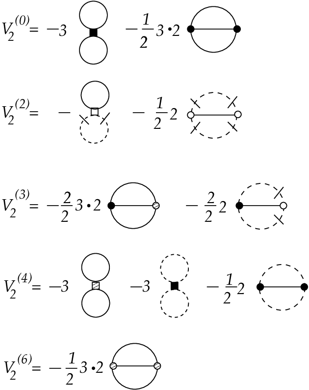
Here, we introduced a power-counting parameter, , in all terms arising from the expansions of the transcendental functions in the Lagrangian (5), in a way that each power of is accompanied by a factor . Our proof of cancellation of infinities will here include terms up to . The classical (tree-level) potential is given by
| (77) |
The CJT effective potential is still given by Eq. (12), but the inverse tree-level propagators now read
| (78) | |||||
| (79) |
where apart from the additional factor of in the mass term of the pion propagator, the tree-level propagator for the sigma receives an additional contribution from the expansion of the logarithm arising from the Jacobian, cf. Eq. (76).
Applying the usual Feynman rules for the construction of the 2PI contribution to the effective potential (12), the latter can now be ordered in powers of accompanying the interaction terms in Eq. (76). Up to two-loop order we obtain
| (80) |
where
| (81) | |||||
| (82) | |||||
| (83) | |||||
| (84) | |||||
| (85) |
Figure 9 shows these terms in a graphical form, including combinatorial factors. The minus signs are due to the fact that the effective potential is proportional to the negative of the pressure. Terms with two identical (different) vertices are of second order in the interaction and thus have an additional factor of 1/2 (2/2). Other factors are of combinatorial origin and denote the number of possibilities to connect the vertices with lines.
The stationarity condition of the effective potential with respect to the one-point function now reads
| (86) | |||||
where the terms in the first line on the right-hand side originate from the one-loop terms in the effective potential, the terms in the second line from , the terms in the third line from , and the terms in the fourth line from . We suppressed terms of higher order, as our proof of cancellation of infinities extends only up to (and including) terms of order .
The stationarity conditions of the effective potential with respect to the two-point functions lead to
| (87) | |||||
| (88) | |||||
At order , the following infinite terms arise in the effective potential: one in the one-loop term [the second term in Eq. (12)], where the inverse tree-level sigma propagator appears, which features a term , cf. Eq. (78), and one in each of the two terms from the two-loop contribution (82). This already demonstrates the above mentioned fact that terms of higher-loop order are required in order to cancel infinities at lower-loop order. We now isolate the infinities in the two-loop terms (82) and prove that they cancel against the one from the one-loop term. To this end, we have to compute these diagrams explicitly.
In a perturbative calculation, it is sufficient to consider the two-point functions appearing in both the aforementioned one-loop term as well as in the terms in Eq. (82) only to order , as each of these terms is already of order . To order , Eqs. (87), (88) reduce to
| (89) | |||||
| (90) |
Plugging this approximate form of the pion propagator into the two terms in the third line of Eq. (87) we obtain after some straightforward steps
| (91) | |||||
The first term on the right-hand side cancels the last term in the first line of Eq. (87), so there are, at least to order , no terms in the two-point function of the sigma particle. One can convince oneself that there are also no infinities in the two-point function of the pion. The same is true for the stationarity condition of the effective potential with respect to the one-point function.
We now proceed to compute the terms in the effective potential, in the approximation (89), (90) for the sigma and pion two-point functions, in order to see the cancellation of infinite terms between the one-loop term involving the tree-level sigma propagator and the two terms of Eq. (82):
| (92) | |||||
where we substituted variables in the last term. The integral in this term has already been computed in the above analysis of the sigma two-point function, cf. Eq. (91). Utilizing this, we obtain
| (93) | |||||
We observe that the terms cancel, as claimed.
Now we would like to show the cancellation of infinities up to order in the effective potential. At two-loop order, there is one term , cf. Eq. (83). As one can convince oneself, this infinite contribution cannot be cancelled by the second term in Eq. (83), which is finite. The cancellation is, however, affected by a term at the three-loop level.

Consider the diagram in Fig. 10. This is of fourth order in interaction vertices, so there is a factor . There are possibilities to attach the sigma lines emerging from the central vertex to the three other vertices on the pion loop. There are possibilities to connect the remaining pion lines to form a diagram with this particular topology. Thus,
where we isolated the integration from the sigma propagators by the substitutions and . The integral can now be computed, using the approximate form of the pion two-point function (90),
| (94) | |||||
where we made frequent use of substitutions of the integration variable. Apart from the last term, the only terms which produce infinities are those where a single pion propagator is accompanied by a factor of . Collecting these, we obtain
| (95) | |||||
As one can see, this term exactly cancels the infinite term in Eq. (83).
References
- [1] H. Kleinert and V. Schulte-Frohlinde. Critical properties of phi**4-theories. (World Scientific, 2001, River Edge, USA).
- [2] H. Meyers-Ortmanns, H.J. Pirner, and B.J. Schaefer. Phys.Lett., B311:213–218, 1993.
- [3] Heui-Seol Roh and T. Matsui. Eur.Phys.J., A1:205–220, 1998.
- [4] Jurgen Baacke and Stefan Michalski. Phys.Rev., D67:085006, 2003.
- [5] Jens O. Andersen, Daniel Boer, and Harmen J. Warringa. Phys.Rev., D70:116007, 2004.
- [6] Nicholas Petropoulos. hep-ph/0402136, 2004.
- [7] Yu.B. Ivanov, F. Riek, and Joern Knoll. Phys.Rev., D71:105016, 2005.
- [8] Bao-Chun Li and Mei Huang. Phys.Rev., D80:034023, 2009.
- [9] E.N. Argyres, M.T.M. van Kessel, and R.H.P. Kleiss. Eur.Phys.J., C64:319–349, 2009.
- [10] Robert D. Pisarski and Frank Wilczek. Phys. Rev., D29:338–341, 1984.
- [11] Frank Wilczek. Int. J. Mod. Phys., A7:3911–3925, 1992.
- [12] Jonathan T. Lenaghan and Dirk H. Rischke. J. Phys., G26:431–450, 2000.
- [13] Agostino Butti, Andrea Pelissetto, and Ettore Vicari. JHEP, 08:029, 2003.
- [14] H. Meyer-Ortmanns and T. Reisz. Principles of phase structures in particle physics. (World Scientific, 2007, Hackensack, USA).
- [15] Elina Seel, Stefan Struber, Francesco Giacosa, and Dirk H. Rischke. Phys.Rev., D86:125010, 2012.
- [16] J. Gasser and H. Leutwyler. Annals Phys., 158:142, 1984.
- [17] G. Ecker, J. Gasser, A. Pich, and E. de Rafael. Nucl.Phys., B321:311, 1989.
- [18] Stefan Scherer. Adv.Nucl.Phys., 27:277, 2003. (eds. J.W. Negele and E. Vogt).
- [19] S. Kamefuchi, L. O’Raifeartaigh, and Abdus Salam. Nucl.Phys., 28:529–549, 1961.
- [20] S. Kondratyuk, A.D. Lahiff, and H.W. Fearing. Phys.Lett., B521:204–210, 2001.
- [21] John M. Cornwall, R. Jackiw, and E. Tomboulis. Phys. Rev., D10:2428–2445, 1974.
- [22] E. N. Argyres, C. G. Papadopoulos, M. T. M. van Kessel, and R. H. P. Kleiss. Eur. Phys. J., C61:495–518, 2009.
- [23] George Leibbrandt. Rev. Mod. Phys., 47:849, 1975.
- [24] H. Kleinert and A. Chervyakov. Eur.Phys.J., C19:743–747, 2001.
- [25] M. Grahl. The model in polar coordinates at nonzero temperature. Diploma thesis, Goethe-University Frankfurt am Main, 2009.
- [26] Hendrik van Hees and Joern Knoll. Phys.Rev., D66:025028, 2002.
- [27] Alexander Bochkarev and Joseph I. Kapusta. Phys.Rev., D54:4066–4079, 1996.
- [28] Stefan Leupold. hep-ph/0407197.
- [29] Jens O. Andersen and Michael Strickland. Ann. Phys., 317:281–353, 2005.
- [30] S. Gasiorowicz and D.A. Geffen. Rev.Mod.Phys., 41:531–573, 1969.
- [31] Pyungwon Ko and Serge Rudaz. Phys.Rev., D50:6877–6894, 1994.
- [32] Stefan Struber and Dirk H. Rischke. Phys.Rev., D77:085004, 2008.
- [33] Denis Parganlija, Francesco Giacosa, and Dirk H. Rischke. Phys.Rev., D82:054024, 2010.