跳到论文正文
W Papers独立论文阅读器 arXiv:1110.2368 论文正文 计算阅读时间 · 0%
引用这篇论文根据当前论文元数据生成,正式投稿前建议核对。


License: arXiv.org perpetual non-exclusive license
arXiv:1110.2368v3 [hep-ph] 24 Jan 2015

The fully differential decay rate of a Higgs boson to bottom-quarks at NNLO in QCD

Achilleas Lazopoulos Affiliation: Institute for Theoretical Physics, ETH Zurich, 8093 Zurich, Switzerland Email: lazopoli@itp.phys.ethz.ch Affiliation: E-mail:
Abstract: 

The decay of a light Higgs boson to bottom quarks is dominant and can be exploited for the discovery of the Higgs particle and the measurement of its properties at the LHC and future collider experiments. We perform a first computation of the fully differential decay at next-next-to-leading order in perturbative QCD. We employ a novel method of non-linear mappings for the treatment of singularities in the radiative processes which contribute to the decay width. This constitutes the first physical application of the method.

Keywords: 
QCD, NLO, NNLO, LHC, Tevatron

1 Introduction

Direct searches and electroweak precision tests suggest that a Standard Model Higgs boson is light, and that it should decay predominantly into a bottom quark (b​b¯b\bar{b}) pair. Inclusive searches at the LHC of a Higgs resonance in the bottom-pair invariant mass distribution are unfortunately hampered by a very large QCD background. Direct searches are focusing on other decay channels, such as H→γ​γH\to\gamma\gamma, with a much smaller branching ratio. In view of this, perturbative corrections to the H→b​b¯H\to b\bar{b} decay are most interesting for the inclusive rate, due to its contribution to the total decay width and the branching ratios of other decays. A remarkable effort has been made for a precise calculation of ΓH→b​b¯\Gamma_{H\to b\bar{b}} and now QCD corrections are known to 𝒪⁡(αs4)\mathcal{O}(\alpha_{s}^{4}) [1, 2, 3, 4, 5, 6, 7, 8, 9].

Recently, confidence has grown that the H→b​b¯H\to b\bar{b} decay can be observed at the LHC directly in events where the Higgs boson is produced in association with a massive vector boson (W,Z)(W,Z) [10] or a t​t¯t\bar{t} pair [11]. Backgrounds from t​t¯t\bar{t},V+j​jV+jj and multi-jet production are challenging. However, the excellent b−b-jet tagging of the ATLAS and CMS detectors as well as sophisticated selections of jet events described in [10, 11], render these channels hopeful, as explicitly demonstrated by the ATLAS collaboration in a full detector simulation analysis for the Z​HZH case [12]. For this channel, further suppression of the background can be obtained with the sub-jet algorithms of [13].

These search strategies rely on a selection of phase space corners which are rich in potential Higgs events. An accurate modeling of QCD radiation is necessary in order to assess the efficiency of these selections. This motivates the computation of the fully differential H→b​b¯H\rightarrow b\bar{b} decay rate at next-to-next-to-leading-order (NNLO) in perturbative QCD.

Next-to-leading-order (NLO) computations [14, 15, 16, 17, 18, 19, 20, 21, 22, 23, 24, 25, 26] are currently performed with very well automated methods [27, 28, 29, 30, 32, 31, 33, 34, 35]. Obtaining fully differential cross-sections and decay rates at one order higher in the perturbative expansion requires the solution of new challenging problems. In the last decade rapid progress [36, 37, 38, 39, 40, 41, 42, 43, 44, 45, 46, 47, 48, 49, 50, 51, 52, 53, 54, 55, 56, 57, 58, 59, 60] with important results [61, 62, 63, 64, 65, 66, 67, 68, 69, 70, 71, 72, 73] has been achieved. However, further developments of methods and new ideas are necessary for efficient cancelations of infrared singularities and evaluations of novel two-loop amplitudes in more complicated LHC processes.

In Ref. [74] we introduced a new method to extract the singularities of multi-dimensional loop and phase space integrals which emerge at NNLO. The method employs non-linear transformations for the factorization of overlapping singularities which in turn allow for an efficient numerical evaluation. In this article, we demonstrate the method in a realistic physical example. We compute for the first time the fully differential decay rate for H→b​b¯H\to b\bar{b} at NNLO.

The paper is organized as follows. In Section 2 we fix our notation and set up the calculation. In Section 3 we present the matrix elements for the processes which contribute to the decay width through NNLO. In Section 4 we describe the parameterization of the phase space for the final state partons. In Section 5 and Section 6 we explain how our method leads to a simple factorizable form for the singularities in the integrals which emerge at NNLO. In Section 7 we present the inclusive width and examples of differential observables with our numerical code.

2 Notation

We compute the partial width ΓH→b​b¯​X​[𝒥]\Gamma_{H\to b\bar{b}X}[{\cal J}] through NNLO in perturbative QCD for any infrared safe observable 𝒥{\cal J}, such as an appropriate jet-algorithm, in the decay of a Higgs boson to a pair of bottom-quarks,

H→b+b¯+X.H\to b+\bar{b}+X. (1)

We consider that the Higgs boson couples to a bottom-quark pair with an unrenormalized Yukawa coupling ybBy_{b}^{B}. Due to the largely different mass of the Higgs boson, mHm_{H}, and the small bottom-quark, mbm_{b}, we treat the latter as independent of the Yukawa coupling and set it to zero, mb=0m_{b}=0, in matrix elements and phase space integrals. In addition, we neglect top-quarks both in virtual corrections and in the renormalization procedure and consider nf=5n_{f}=5 light quark flavors. For the renormalization of ultraviolet (UV) divergences we work in the MS¯\overline{\rm{MS}}-scheme where the bare couplings, ybBy_{b}^{B}, and gsB=4​π​αsBg_{s}^{B}=\sqrt{4\pi\alpha_{s}^{B}}, are related to their renormalized counterparts through the following relations:

ybB\displaystyle y_{b}^{B} =\displaystyle= yb[1−αs4​π3​CFϵ+(αs4​π)2[−1ϵ2(2TFnf−92CF−112CA)\displaystyle y_{b}\Bigg[1-\frac{\alpha_{s}}{4\pi}\frac{3C_{F}}{\epsilon}+\left(\frac{\alpha_{s}}{4\pi}\right)^{2}\Big[-\frac{1}{\epsilon^{2}}\left(2T_{F}n_{f}-\frac{9}{2}C_{F}-\frac{11}{2}C_{A}\right) (2)
+1ϵ(5​TF3nf−3​CF4−9712CA)]CF+𝒪(αs3)]\displaystyle+\frac{1}{\epsilon}\left(\frac{5T_{F}}{3}n_{f}-\frac{3C_{F}}{4}-\frac{97}{12}C_{A}\right)\Big]C_{F}+\mathcal{O}(\alpha_{s}^{3})\Bigg]
αsB\displaystyle\alpha_{s}^{B} =\displaystyle= αs​(μ2​eγE4​π)ϵ​[1−αs4​π​1ϵ​[11​CA3−4​TF​nf3]+𝒪⁡(αs2)].\displaystyle\alpha_{s}\left(\frac{\mu^{2}e^{\gamma_{E}}}{4\pi}\right)^{\epsilon}\left[1-\frac{\alpha_{s}}{4\pi}\frac{1}{\epsilon}\left[\frac{11C_{A}}{3}-\frac{4T_{F}n_{f}}{3}\right]+\mathcal{O}(\alpha_{s}^{2})\right]. (3)

The renormalized strong coupling and Higgs Yukawa coupling depend implicitly on the renormalization scale μ\mu,

αs≡αs​(μ)yb≡yb​(μ).\alpha_{s}\equiv\alpha_{s}(\mu)\quad y_{b}\equiv y_{b}(\mu). (4)

The SU(N) Casimirs are given by

CA=N,CF=N2−12​N,TF=12,C_{A}=N,\quad C_{F}=\frac{N^{2}-1}{2N},\quad T_{F}=\frac{1}{2}, (5)

where N=3N=3 is the number of quark colors.

Through NNLO, the partial decay width receives contributions from the following partonic processes:

  • •

    H⁡(pH)→b⁡(p1)​b¯​(p2)H(p_{H})\to b(p_{1})\bar{b}(p_{2}) at two loops,

  • •

    H⁡(pH)→b⁡(p1)​b¯​(p2)​g​(p3)H(p_{H})\to b(p_{1})\bar{b}(p_{2})g(p_{3}) at one loop and

  • •

    H⁡(pH)→b⁡(p1)​b¯​(p2)​g​(p3)​g​(p4),b⁡(p1)​b¯​(p2)​b​(p3)​b¯​(p4),b⁡(p1)​b¯​(p2)​q​(p3)​q¯​(p4)H(p_{H})\to b(p_{1})\bar{b}(p_{2})g(p_{3})g(p_{4}),b(p_{1})\bar{b}(p_{2})b(p_{3})\bar{b}(p_{4}),b(p_{1})\bar{b}(p_{2})q(p_{3})\bar{q}(p_{4}) with q≠bq\neq b at tree level,

where in parenthesis we indicate the four-momenta of the corresponding particles. The width is the sum

ΓH→b​b¯​X​[𝒥]\displaystyle\Gamma_{H\to b\bar{b}X}[{\cal J}] =\displaystyle= ΓH→b​b¯​[𝒥]\displaystyle\Gamma_{H\to b\bar{b}}[{\cal J}] (6)
+\displaystyle+ ΓH→b​b¯​g​[𝒥]\displaystyle\Gamma_{H\to b\bar{b}g}[{\cal J}]
+\displaystyle+ ΓH→b​b¯​g​g​[𝒥]+(nf−1)⋅ΓH→b​b¯​q​q​[𝒥]+ΓH→b​b¯​b​b¯​[𝒥]\displaystyle\Gamma_{H\to b\bar{b}gg}[{\cal J}]+(n_{f}-1)\cdot\Gamma_{H\to b\bar{b}qq}[{\cal J}]+\Gamma_{H\to b\bar{b}b\bar{b}}[{\cal J}]
+\displaystyle+ 𝒪⁡(αs3),\displaystyle{\cal O}(\alpha_{s}^{3}),

where

ΓH→b​b¯​[𝒥]\displaystyle\Gamma_{H\to b\bar{b}}[{\cal J}] =\displaystyle= 12​mH​∫d​Φ2​∑spin|ℳH→b⁡(p1)+b¯​(p2)|2​𝒥​(p1,p2),\displaystyle\frac{1}{2m_{H}}\int d\Phi_{2}\sum_{{\rm spin}}\left|{\cal M}_{H\to b(p_{1})+\bar{b}(p_{2})}\right|^{2}{\cal J}(p_{1},p_{2}),
ΓH→b​b¯​g​[𝒥]\displaystyle\Gamma_{H\to b\bar{b}g}[{\cal J}] =\displaystyle= 12​mH​∫d​Φ3​∑spin|ℳH→b⁡(p1)+b¯​(p2)+g⁡(p3)|2​𝒥​(p1,p2,p3),\displaystyle\frac{1}{2m_{H}}\int d\Phi_{3}\sum_{{\rm spin}}\left|{\cal M}_{H\to b(p_{1})+\bar{b}(p_{2})+g(p_{3})}\right|^{2}{\cal J}(p_{1},p_{2},p_{3}),
ΓH→b​b¯​g​g​[𝒥]\displaystyle\Gamma_{H\to b\bar{b}gg}[{\cal J}] =\displaystyle= 12​mH​∫d​Φ4​∑spin|ℳH→b⁡(p1)+b¯​(p2)+g⁡(p3)+g⁡(p4)|2⋅12!⋅𝒥⁡(p1,p2,p3,p4),\displaystyle\frac{1}{2m_{H}}\int d\Phi_{4}\sum_{{\rm spin}}\left|{\cal M}_{H\to b(p_{1})+\bar{b}(p_{2})+g(p_{3})+g(p_{4})}\right|^{2}\cdot\frac{1}{2!}\cdot{\cal J}(p_{1},p_{2},p_{3},p_{4}),
ΓH→b​b¯​b​b¯​[𝒥]\displaystyle\Gamma_{H\to b\bar{b}b\bar{b}}[{\cal J}] =\displaystyle= 12​mH​∫d​Φ4​∑spin|ℳH→b⁡(p1)+b¯​(p2)+b⁡(p3)+b¯​(p4)|2⋅1(2!)2⋅𝒥⁡(p1,p2,p3,p4),\displaystyle\frac{1}{2m_{H}}\int d\Phi_{4}\sum_{{\rm spin}}\left|{\cal M}_{H\to b(p_{1})+\bar{b}(p_{2})+b(p_{3})+\bar{b}(p_{4})}\right|^{2}\cdot\frac{1}{(2!)^{2}}\cdot{\cal J}(p_{1},p_{2},p_{3},p_{4}),
ΓH→b​b¯​q​q¯​[𝒥]\displaystyle\Gamma_{H\to b\bar{b}q\bar{q}}[{\cal J}] =\displaystyle= 12​mH​∫d​Φ4​∑spin|ℳH→b⁡(p1)+b¯​(p2)+q⁡(p3)+q¯​(p4)|2​𝒥​(p1,p2,p3,p4).\displaystyle\frac{1}{2m_{H}}\int d\Phi_{4}\sum_{{\rm spin}}\left|{\cal M}_{H\to b(p_{1})+\bar{b}(p_{2})+q(p_{3})+\bar{q}(p_{4})}\right|^{2}{\cal J}(p_{1},p_{2},p_{3},p_{4}). (7)

In the above, we integrate the appropriate matrix elements computed in conventional dimensional regularization (CDR) over the phase space in D=4−2​ϵD=4-2\epsilon dimensions of the final-state partons and the function 𝒥{\cal J} defining an infrared safe observable. The phase space measure reads

d​Φn≡(2​π)D​δ(D)​(pH−∑i=1npi)​∏i=1ndD​pi(2​π)D−1​δ(+)​(pi2).d\Phi_{n}\equiv(2\pi)^{D}\delta^{(D)}\left(p_{H}-\sum_{i=1}^{n}p_{i}\right)\prod_{i=1}^{n}\frac{d^{D}p_{i}}{\left(2\pi\right)^{D-1}}\delta^{(+)}(p_{i}^{2}). (8)

Lorentz invariants are defined as

mH2=pH2,si​j=2​pi.pj,si​j​k=si​j+si​k+sj​k.m_{H}^{2}=p_{H}^{2},\quad s_{ij}=2p_{i}.p_{j},\quad s_{ijk}=s_{ij}+s_{ik}+s_{jk}. (9)

Regarding the analytic continuations of complex functions presented in this paper the positive “epsilon prescription” must be used, since all occurring mass scales are external,i.e.

mH2→mH2+i​ε,si​j→si​j+i​ε.m_{H}^{2}\rightarrow m_{H}^{2}+i\varepsilon,\quad s_{ij}\rightarrow s_{ij}+i\varepsilon. (10)

where ε\varepsilon is a small positive parameter.

3 Matrix elements

In this section we present the square of the scattering amplitudes needed for the computation of the H→b​b¯H\rightarrow b\bar{b} decay width through 𝒪⁡(αs​(μ)2)\mathcal{O}(\alpha_{s}(\mu)^{2}). These can be easily derived with modern methods for computing Feynman diagrams and have been ingredients of many prior calculations. For example, the same matrix elements enter the calculation of the NNLO total cross-section b​b¯→Hb\bar{b}\to H [75]. We have made an independent computation and present them here for completeness. For the generation of the matrix elements we used QGRAF [76]. For further symbolic manipulations, such as color and Dirac algebra, we used FORM [77] and MAPLE [78]. We reduced one and two-loop amplitudes to master integrals using the method of integration by parts [79, 80] and the Laporta algorithm [81] with AIR [82].

3.1 Decay to two partons

For the process

H⁡(pH)→b⁡(p1)+b¯​(p2)H(p_{H})\rightarrow b(p_{1})+\bar{b}(p_{2})

we require up to 2-loop corrections:

|ℳH→b​b¯|2=2​yb​(μ)2​mH2​N​[1+αs​(μ)π​𝒜H→b​b¯(1)+(αs​(μ)π)2​𝒜H→b​b¯(2)+𝒪⁡(αs​(μ)3)],\left|\mathcal{M}_{H\rightarrow b\bar{b}}\right|^{2}=2y_{b}(\mu)^{2}m_{H}^{2}N\left[1+\frac{\alpha_{s}(\mu)}{\pi}\mathcal{A}_{H\rightarrow b\bar{b}}^{(1)}+\left(\frac{\alpha_{s}(\mu)}{\pi}\right)^{2}\mathcal{A}_{H\rightarrow b\bar{b}}^{(2)}+\mathcal{O}(\alpha_{s}(\mu)^{3})\right], (11)

where (let ℜ⁡(z)\Re(z) shall denote the real part of zz)

𝒜H→b​b¯(1)=−CF​[ℜ⁡((μ2−mH2)ϵ)​fϵ+32​ϵ]\mathcal{A}_{H\rightarrow b\bar{b}}^{(1)}=-C_{F}\Bigg[\Re\left(\left(\frac{\mu^{2}}{-m_{H}^{2}}\right)^{\epsilon}\right)f_{\epsilon}+\frac{3}{2\epsilon}\Bigg]

with

fϵ=(1−ϵ)2​Γ⁡(1+ϵ)​Γ​(−ϵ)2Γ⁡(2−2​ϵ)​eγ​ϵ.f_{\epsilon}=(1-\epsilon)^{2}\frac{\Gamma(1+\epsilon)\Gamma(-\epsilon)^{2}}{\Gamma(2-2\epsilon)}e^{\gamma\epsilon}. (12)

The 𝒪⁡(αs​(μ)2)\mathcal{O}(\alpha_{s}(\mu)^{2}) contribution can be split into two pieces

𝒜H→b​b¯(2)=𝒜H→b​b¯V​V+𝒜H→b​b¯V2\displaystyle\mathcal{A}_{H\rightarrow b\bar{b}}^{(2)}=\mathcal{A}_{H\rightarrow b\bar{b}}^{VV}+\mathcal{A}_{H\rightarrow b\bar{b}}^{V^{2}} (13)

corresponding to the one-loop squared amplitude

𝒜H→b​b¯V2=CF24​[|μ2−mH2|2​ϵ​fϵ2+3ϵ​ℜ⁡((μ2−mH2)ϵ)​fϵ+94​ϵ2].\mathcal{A}_{H\rightarrow b\bar{b}}^{V^{2}}=\frac{C_{F}^{2}}{4}\left[\left|\frac{\mu^{2}}{-m_{H}^{2}}\right|^{2\epsilon}f_{\epsilon}^{2}+\frac{3}{\epsilon}\Re\left(\left(\frac{\mu^{2}}{-m_{H}^{2}}\right)^{\epsilon}\right)f_{\epsilon}+\frac{9}{4\epsilon^{2}}\right]. (14)

and the two-loop amplitude interfered with the tree amplitude

𝒜H→b​b¯V​V=[𝒜−4V​Vϵ4+𝒜−3V​Vϵ3+𝒜2V​Vϵ2+𝒜−1V​Vϵ+𝒜0V​V]\mathcal{A}_{H\rightarrow b\bar{b}}^{VV}=\left[\frac{\mathcal{A}^{VV}_{-4}}{\epsilon^{4}}+\frac{\mathcal{A}^{VV}_{-3}}{\epsilon^{3}}+\frac{\mathcal{A}^{VV}_{2}}{\epsilon^{2}}+\frac{\mathcal{A}^{VV}_{-1}}{\epsilon}+\mathcal{A}^{VV}_{0}\right] (15)

where

𝒜0V​V\displaystyle\mathcal{A}_{0}^{VV} =\displaystyle= [1/6lH4+1372lH3+(−6ζ(2)−3136)lH2+(−55108−6124ζ(2)−7/6ζ(3))lH\displaystyle\Bigg[1/6\,{l_{{H}}}^{4}+{\frac{13}{72}}\,{l_{{H}}}^{3}+\left(-6\,\zeta\left(2\right)-{\frac{31}{36}}\right){l_{{H}}}^{2}+\left(-{\frac{55}{108}}-{\frac{61}{24}}\,\zeta\left(2\right)-7/6\,\zeta\left(3\right)\right)l_{{H}}
+455162+37772ζ(2)+26316ζ(4)−4736ζ(3)]CF2\displaystyle+{\frac{455}{162}}+{\frac{377}{72}}\,\zeta\left(2\right)+{\frac{263}{16}}\,\zeta\left(4\right)-{\frac{47}{36}}\,\zeta\left(3\right)\Bigg]{C_{{F}}}^{2}
+[−1/36nflH3+536nflH2+1/27(9ζ(2)−7)nflH\displaystyle+\Bigg[-1/36\,n_{{f}}{l_{{H}}}^{3}+{\frac{5}{36}}\,n_{{f}}{l_{{H}}}^{2}+1/27\,\left(9\,\zeta\left(2\right)-7\right)n_{{f}}l_{{H}}
−1648(495ζ(2)−18ζ(3)−200)nf]CF\displaystyle-{\frac{1}{648}}\,\left(495\,\zeta\left(2\right)-18\,\zeta\left(3\right)-200\right)n_{{f}}\Bigg]C_{{F}}
+[1172lH3+(1/4ζ(2)−6772)lH2+(−134ζ(3)−116ζ(2)+121108)lH\displaystyle+\Bigg[{\frac{11}{72}}\,{l_{{H}}}^{3}+\left(1/4\,\zeta\left(2\right)-{\frac{67}{72}}\right){l_{{H}}}^{2}+\left(-{\frac{13}{4}}\,\zeta\left(3\right)-{\frac{11}{6}}\,\zeta\left(2\right)+{\frac{121}{108}}\right)l_{{H}}
+701144ζ(2)−ζ(4)−467648+15172ζ(3)]CFN−1\displaystyle+{\frac{701}{144}}\,\zeta\left(2\right)-\zeta\left(4\right)-{\frac{467}{648}}+{\frac{151}{72}}\,\zeta\left(3\right)\Bigg]C_{{F}}{N}^{-1}
𝒜−1V​V\displaystyle\mathcal{A}_{-1}^{VV} =\displaystyle= (−1/3lH3+3/8lH2+(6ζ(2)+3136)lH−134ζ(2)+712ζ(3)−491864)CF2\displaystyle\left(-1/3\,{l_{{H}}}^{3}+3/8\,{l_{{H}}}^{2}+\left(6\,\zeta\left(2\right)+{\frac{31}{36}}\right)l_{{H}}-{\frac{13}{4}}\,\zeta\left(2\right)+{\frac{7}{12}}\,\zeta\left(3\right)-{\frac{491}{864}}\right){C_{{F}}}^{2}
+(−536​nf​lH+1432​(54​ζ​(2)+65)​nf)​CF\displaystyle+\left(-{\frac{5}{36}}\,n_{{f}}l_{{H}}+{\frac{1}{432}}\,\left(54\,\zeta\left(2\right)+65\right)n_{{f}}\right)C_{{F}}
+((−1/4ζ(2)+6772)lH−1116ζ(2)+138ζ(3)−961864)CFN−1\displaystyle+\left(\left(-1/4\,\zeta\left(2\right)+{\frac{67}{72}}\right)l_{{H}}-{\frac{11}{16}}\,\zeta\left(2\right)+{\frac{13}{8}}\,\zeta\left(3\right)-{\frac{961}{864}}\right)C_{{F}}{N}^{-1}
𝒜−2V​V\displaystyle\mathcal{A}_{-2}^{VV} =\displaystyle= (−3​ζ​(2)−5/3​lH+1/2​lH2+217144)​CF2\displaystyle\left(-3\,\zeta\left(2\right)-5/3\,l_{{H}}+1/2\,{l_{{H}}}^{2}+{\frac{217}{144}}\right){C_{{F}}}^{2}
+(1/12​nf​lH−1/18​nf)​CF+(1/8​ζ​(2)−1124​lH+2/9)​CF​N−1\displaystyle+\left(1/12\,n_{{f}}l_{{H}}-1/18\,n_{{f}}\right)C_{{F}}+\left(1/8\,\zeta\left(2\right)-{\frac{11}{24}}\,l_{{H}}+2/9\right)C_{{F}}{N}^{-1}
𝒜−3V​V\displaystyle\mathcal{A}_{-3}^{VV} =\displaystyle= (178−1/2​lH)​CF2−1/8​CF​nf+1116​CFN\displaystyle\left({\frac{17}{8}}-1/2\,l_{{H}}\right){C_{{F}}}^{2}-1/8\,C_{{F}}n_{{f}}+{\frac{11}{16}}\,{\frac{C_{{F}}}{N}}
𝒜−4V​V\displaystyle\mathcal{A}_{-4}^{VV} =\displaystyle= 1/4​CF2\displaystyle 1/4\,{C_{{F}}}^{2} (16)

with lH=ln⁡(mH2μ2)l_{H}=\ln\left(\frac{m_{H}^{2}}{\mu^{2}}\right).

3.2 Decay to three partons

For the process

H⁡(pH)→b⁡(p1)+b¯​(p2)+g⁡(p3)H(p_{H})\rightarrow b(p_{1})+\bar{b}(p_{2})+g(p_{3})

we require up to 1-loop corrections:

|ℳH→b​b¯​g|2=yb​(μ)2​[αs​(μ)π​𝒜H→b​b¯​g(0)+(αs​(μ)π)2​𝒜H→b​b¯​g(1)+𝒪⁡(αs​(μ)3)].\left|\mathcal{M}_{H\rightarrow b\bar{b}g}\right|^{2}=y_{b}(\mu)^{2}\left[\frac{\alpha_{s}(\mu)}{\pi}\mathcal{A}_{H\rightarrow b\bar{b}g}^{(0)}+\left(\frac{\alpha_{s}(\mu)}{\pi}\right)^{2}\mathcal{A}_{H\rightarrow b\bar{b}g}^{(1)}+\mathcal{O}(\alpha_{s}(\mu)^{3})\right]. (17)

The tree contribution can be expressed as

𝒜H→b​b¯​g(0)=mH2​N​(4​π)2​(μ2​eγE4​π)ϵ​P^q​q​(s12mH2)​[1s13+1s23]\mathcal{A}_{H\rightarrow b\bar{b}g}^{(0)}=m_{H}^{2}N(4\pi)^{2}\left(\frac{\mu^{2}e^{\gamma_{E}}}{4\pi}\right)^{\epsilon}\hat{P}_{qq}\left(\frac{s_{12}}{m_{H}^{2}}\right)\left[\frac{1}{s_{13}}+\frac{1}{s_{23}}\right] (18)

where

P^q​q​(z)=CF​[1+z21−z−ϵ⁡(1−z)]\hat{P}_{qq}(z)=C_{F}\left[\frac{1+z^{2}}{1-z}-\epsilon(1-z)\right] (19)

is the quark gluon splitting kernel. The one-loop correction can be expressed as

𝒜H→b​b¯​g(1)=π2​(μ2​eγE)2​ϵ(4​π)ϵ×{(8(s23+s13)2​ϵ2s23​s13\displaystyle\mathcal{A}_{H\rightarrow b\bar{b}g}^{(1)}=\frac{\pi^{2}\left(\mu^{2}e^{\gamma_{E}}\right)^{2\epsilon}}{(4\pi)^{\epsilon}}\times\Bigg\{\Bigg(8\,{\frac{\left(s_{23}+s_{13}\right)^{2}{\epsilon}^{2}}{s_{23}s_{13}}}
OPEN+4​(s23+s13)2​ϵs23​s13+−12​s122−12​mH4+8​s12​mH2s23​s13+4​s122+4​mH4ϵ​s13​s23)​CF​Bub​(s12)\displaystyle+4\,{\frac{\left(s_{23}+s_{13}\right)^{2}\epsilon}{s_{23}s_{13}}}+{\frac{-12\,{s_{12}}^{2}-12\,m_{H}^{4}+8\,s_{12}m_{H}^{2}}{s_{23}s_{13}}}+{\frac{4\,{s_{12}}^{2}+4\,m_{H}^{4}}{\epsilon\,s_{13}s_{23}}}\Bigg)C_{F}\,{\rm Bub}\left(s_{12}\right)
+[(8+4(s23+s13)​(s23+mH2)​ϵ2(s13+s12)​s23−4(s12​s23+3​s23​s13−s232+mH4)​ϵ(s13+s12)​s23)NCF2\displaystyle+\Bigg[\Bigg(8+4\,{\frac{\left(s_{23}+s_{13}\right)\left(s_{23}+m_{H}^{2}\right){\epsilon}^{2}}{\left(s_{13}+s_{12}\right)s_{23}}}-4\,{\frac{\left(s_{12}s_{23}+3\,s_{23}s_{13}-{s_{23}}^{2}+m_{H}^{4}\right)\epsilon}{\left(s_{13}+s_{12}\right)s_{23}}}\Bigg)N{C_{F}}^{2}
+(4​(s23+s13)​(2​s23+s13)​ϵ2s23​s13−4​(s12​s13−s232−s132)​ϵs23​s13CLOSE\displaystyle+\Bigg(4\,{\frac{\left(s_{23}+s_{13}\right)\left(2\,s_{23}+s_{13}\right){\epsilon}^{2}}{s_{23}s_{13}}}-4\,{\frac{\left(s_{12}s_{13}-{s_{23}}^{2}-{s_{13}}^{2}\right)\epsilon}{s_{23}s_{13}}}
−42​s122+s232+s23​s13+s132+2​mH4s23​s13+4s122+mH4ϵ​s13​s23)CF]Bub(s23)\displaystyle-4\,{\frac{2\,{s_{12}}^{2}+{s_{23}}^{2}+s_{23}s_{13}+{s_{13}}^{2}+2\,m_{H}^{4}}{s_{23}s_{13}}}+4\,{\frac{{s_{12}}^{2}+m_{H}^{4}}{\epsilon\,s_{13}s_{23}}}\Bigg)C_{F}\Bigg]{\rm Bub}\left(s_{23}\right)
+[(8+4(s23+s13)​(s13+mH2)​ϵ2(s23+s12)​s13−4(s12​s13+3​s23​s13−s132+mH4)​ϵ(s23+s12)​s13)NCF2\displaystyle+\Bigg[\left(8+4\,{\frac{\left(s_{23}+s_{13}\right)\left(s_{13}+m_{H}^{2}\right){\epsilon}^{2}}{\left(s_{23}+s_{12}\right)s_{13}}}-4\,{\frac{\left(s_{12}s_{13}+3\,s_{23}s_{13}-{s_{13}}^{2}+m_{H}^{4}\right)\epsilon}{\left(s_{23}+s_{12}\right)s_{13}}}\right)N{C_{F}}^{2}
+(4​(s23+2​s13)​(s23+s13)​ϵ2s23​s13−4​(s12​s23−s232−s132)​ϵs23​s13CLOSE\displaystyle+\Bigg(4\,{\frac{\left(s_{23}+2\,s_{13}\right)\left(s_{23}+s_{13}\right){\epsilon}^{2}}{s_{23}s_{13}}}-4\,{\frac{\left(s_{12}s_{23}-{s_{23}}^{2}-{s_{13}}^{2}\right)\epsilon}{s_{23}s_{13}}}
−42​s122+s232+s23​s13+s132+2​mH4s23​s13+4s122+mH4ϵ​s13​s23)CF]Bub(s13)\displaystyle-4\,{\frac{2\,{s_{12}}^{2}+{s_{23}}^{2}+s_{23}s_{13}+{s_{13}}^{2}+2\,m_{H}^{4}}{s_{23}s_{13}}}+4\,{\frac{{s_{12}}^{2}+m_{H}^{4}}{\epsilon\,s_{13}s_{23}}}\Bigg)C_{F}\Bigg]{\rm Bub}\left(s_{13}\right)
+[(−8(s23+s13)​mH2​(2​s23​s13+s12​s23+s12​s13)​ϵ2s13​s23​(s23+s12)​(s13+s12)−82​s122+3​s23​s13+s232+s132+2​mH4s23​s13\displaystyle+\Bigg[\Bigg(-8\,{\frac{\left(s_{23}+s_{13}\right)m_{H}^{2}\left(2\,s_{23}s_{13}+s_{12}s_{23}+s_{12}s_{13}\right){\epsilon}^{2}}{s_{13}s_{23}\left(s_{23}+s_{12}\right)\left(s_{13}+s_{12}\right)}}-8\,{\frac{2\,{s_{12}}^{2}+3\,s_{23}s_{13}+{s_{23}}^{2}+{s_{13}}^{2}+2\,m_{H}^{4}}{s_{23}s_{13}}}
+(8​mH24−8​s122​s132+16​s232​s132−8​s232​s122+8​s124−8​s133​mH2−8​s233​mH2)​ϵs13​s23​(s23+s12)​(s13+s12)\displaystyle+{\frac{\left(8\,{m_{H}^{2}}^{4}-8\,{s_{12}}^{2}{s_{13}}^{2}+16\,{s_{23}}^{2}{s_{13}}^{2}-8\,{s_{23}}^{2}{s_{12}}^{2}+8\,{s_{12}}^{4}-8\,{s_{13}}^{3}m_{H}^{2}-8\,{s_{23}}^{3}m_{H}^{2}\right)\epsilon}{s_{13}s_{23}\left(s_{23}+s_{12}\right)\left(s_{13}+s_{12}\right)}}
OPEN+8​s122+mH22ϵ​s13​s23)​N​CF2+(−8​(s23+s13)2​ϵ2s23​s13−4​(s232+s132)​ϵs23​s13CLOSE\displaystyle+8\,{\frac{{s_{12}}^{2}+{m_{H}^{2}}^{2}}{\epsilon\,s_{13}s_{23}}}\Bigg)N{C_{F}}^{2}+\Bigg(-8\,{\frac{\left(s_{23}+s_{13}\right)^{2}{\epsilon}^{2}}{s_{23}s_{13}}}-4\,{\frac{\left({s_{23}}^{2}+{s_{13}}^{2}\right)\epsilon}{s_{23}s_{13}}}
+42​s122+s232+s23​s13+s132+2​mH4s23​s13−4s122+mH4ϵ​s13​s23)CF]Bub(mH2)\displaystyle+4\,{\frac{2\,{s_{12}}^{2}+{s_{23}}^{2}+s_{23}s_{13}+{s_{13}}^{2}+2\,m_{H}^{4}}{s_{23}s_{13}}}-4\,{\frac{{s_{12}}^{2}+m_{H}^{4}}{\epsilon\,s_{13}s_{23}}}\Bigg)C_{F}\Bigg]{\rm Bub}\left(m_{H}^{2}\right)
+(2​s12​s13​(s23+s13)​ϵ2s23+2​s12​(s23+s13)2​ϵs23−2​s12​(s122+mH4)s23)​CF​Box​(s12,s13,mH2)\displaystyle+\left(2\,{\frac{s_{12}s_{13}\left(s_{23}+s_{13}\right){\epsilon}^{2}}{s_{23}}}+2\,{\frac{s_{12}\left(s_{23}+s_{13}\right)^{2}\epsilon}{s_{23}}}-2\,{\frac{s_{12}\left({s_{12}}^{2}+m_{H}^{4}\right)}{s_{23}}}\right)C_{F}\,{\rm Box}\left(s_{12},s_{13},m_{H}^{2}\right)
+(2​s12​s23​(s23+s13)​ϵ2s13+2​s12​(s23+s13)2​ϵs13−2​s12​(s122+mH4)s13)​CF​Box​(s23,s12,mH2)\displaystyle+\left(2\,{\frac{s_{12}s_{23}\left(s_{23}+s_{13}\right){\epsilon}^{2}}{s_{13}}}+2\,{\frac{s_{12}\left(s_{23}+s_{13}\right)^{2}\epsilon}{s_{13}}}-2\,{\frac{s_{12}\left({s_{12}}^{2}+m_{H}^{4}\right)}{s_{13}}}\right)C_{F}\,{\rm Box}\left(s_{23},s_{12},m_{H}^{2}\right)
+[((−12s23s13−4s232−4s132)ϵ+4s122+4mH4)NCF2\displaystyle+\Big[\left(\left(-12\,s_{23}s_{13}-4\,{s_{23}}^{2}-4\,{s_{13}}^{2}\right)\epsilon+4\,{s_{12}}^{2}+4\,m_{H}^{4}\right)N{C_{F}}^{2}
+((−6s23s13−2s232−2s132)ϵ+2s122+2mH4)CF]Box(s13,s23,mH2)}\displaystyle+\left(\left(-6\,s_{23}s_{13}-2\,{s_{23}}^{2}-2\,{s_{13}}^{2}\right)\epsilon+2\,{s_{12}}^{2}+2\,m_{H}^{4}\right)C_{F}\Big]{\rm Box}\left(s_{13},s_{23},m_{H}^{2}\right)\Bigg\}
−1ϵ​(3​CF2+11​CA12−TF​nf3)​𝒜H→b​b¯​g(0).\displaystyle-\frac{1}{\epsilon}\left(\frac{3C_{F}}{2}+\frac{11C_{A}}{12}-\frac{T_{F}n_{f}}{3}\right)\mathcal{A}_{H\rightarrow b\bar{b}g}^{(0)}. (20)

There are only two different master integrals which appear here. The bubble

Bub⁡(s23)=∫dd​ki​πd2​1k2​(k+p23)2=Γ⁡(1+ϵ)​Γ​(1−ϵ)2ϵ​Γ​(2−2​ϵ)​(−s23)−ϵ{\rm Bub}(s_{23})=\int\frac{d^{d}k}{i\pi^{\frac{d}{2}}}\frac{1}{k^{2}(k+p_{23})^{2}}=\frac{\Gamma(1+\epsilon)\Gamma(1-\epsilon)^{2}}{\epsilon\Gamma(2-2\epsilon)}(-s_{23})^{-\epsilon} (21)

as well as the following box integral

Box⁡(s23,s34,mH2)=∫dd​ki​πd2​1k2​(k+p2)2​(k+p23)2​(k+p234)2.{\rm Box}(s_{23},s_{34},m_{H}^{2})=\int\frac{d^{d}k}{i\pi^{\frac{d}{2}}}\frac{1}{k^{2}(k+p_{2})^{2}(k+p_{23})^{2}(k+p_{234})^{2}}. (22)

which can be expressed to all orders in ϵ\epsilon in terms of hypergeometric functions

Box⁡(s,t,M2)\displaystyle{\rm Box}\left(s,t,M^{2}\right) =\displaystyle= 2​Γ​(1+ϵ)​Γ​(1−ϵ)2ϵ2​Γ​(1−2​ϵ)1s​t[−(−M2)−ϵF12(1,−ϵ,1−ϵ,−u​M2s​t)\displaystyle\frac{2\Gamma(1+\epsilon)\Gamma(1-\epsilon)^{2}}{\epsilon^{2}\Gamma(1-2\epsilon)}\frac{1}{st}\Bigg[-(-M^{2})^{-\epsilon}{}_{2}F_{1}(1,-\epsilon,1-\epsilon,-\frac{uM^{2}}{st}) (23)
+\displaystyle+ (−t)−ϵF12(1,−ϵ,1−ϵ,−us)+(−s)−ϵF12(1,−ϵ,1−ϵ,−ut)]\displaystyle(-t)^{-\epsilon}{}_{2}F_{1}(1,-\epsilon,1-\epsilon,-\frac{u}{s})+(-s)^{-\epsilon}{}_{2}F_{1}(1,-\epsilon,1-\epsilon,-\frac{u}{t})\Bigg]

with u=M2−s−tu=M^{2}-s-t.

3.3 Decay to four partons

For the decay to four partons we need

H⁡(pH)→b⁡(p1)+b¯​(p2)+i⁡(p3)+j⁡(p4),(i​j)∈{(q​q¯),(b​b¯),(g​g)}H(p_{H})\rightarrow b(p_{1})+\bar{b}(p_{2})+i(p_{3})+j(p_{4}),\quad(ij)\in\{(q\bar{q}),(b\bar{b}),(gg)\} (24)

at tree-level

|ℳH→b​b¯​i​j|2=yb​(μ)2​(αs​(μ)π)2​𝒜H→b​b¯​i​j(0)+𝒪⁡(αs​(μ)3).\left|\mathcal{M}_{H\rightarrow b\bar{b}ij}\right|^{2}=y_{b}(\mu)^{2}\left(\frac{\alpha_{s}(\mu)}{\pi}\right)^{2}\mathcal{A}_{H\rightarrow b\bar{b}ij}^{(0)}+\mathcal{O}(\alpha_{s}(\mu)^{3}). (25)

The H→b​b¯​q​q¯H\rightarrow b\bar{b}q\bar{q} amplitude can be expressed as

𝒜H→b​b¯​q​q¯(0)=16​π4​(μ2​eγE4​π)2​ϵ​[2​N​CF​A​(p1,p2,p3,p4)]\mathcal{A}_{H\rightarrow b\bar{b}q\bar{q}}^{(0)}=16\pi^{4}\left(\frac{\mu^{2}e^{\gamma_{E}}}{4\pi}\right)^{2\epsilon}\left[2NC_{F}A(p_{1},p_{2},p_{3},p_{4})\right] (26)

while for two b​b¯b\bar{b} pairs in the final state we get

𝒜H→b​b¯​b​b¯(0)\displaystyle\mathcal{A}_{H\rightarrow b\bar{b}b\bar{b}}^{(0)} =\displaystyle= 16π4(μ2​eγE4​π)2​ϵ×\displaystyle 16\pi^{4}\left(\frac{\mu^{2}e^{\gamma_{E}}}{4\pi}\right)^{2\epsilon}\times (27)
{2NCF[A(p1,p2,p3,p4)+A(p1,p4,p3,p2)+A(p3,p2,p1,p4)+A(p3,p4,p1,p2)]\displaystyle\Bigg\{2NC_{F}\left[A(p_{1},p_{2},p_{3},p_{4})+A(p_{1},p_{4},p_{3},p_{2})+A(p_{3},p_{2},p_{1},p_{4})+A(p_{3},p_{4},p_{1},p_{2})\right]
+2CF[B(p1,p2,p3,p4)+B(p3,p4,p1,p2)+B(p4,p3,p2,p1)+B(p2,p1,p4,p3)]}\displaystyle+2C_{F}\left[B(p_{1},p_{2},p_{3},p_{4})+B(p_{3},p_{4},p_{1},p_{2})+B(p_{4},p_{3},p_{2},p_{1})+B(p_{2},p_{1},p_{4},p_{3})\right]\Bigg\}

where

A⁡(p1,p2,p3,p4)\displaystyle A(p_{1},p_{2},p_{3},p_{4}) =\displaystyle= 2[2​(1−ϵ)s34−(1+ϵ)(1s134+1s234)+m2(ϵ−1)(1s1342+1s2342)\displaystyle 2\bigg[\frac{2(1-\epsilon)}{s_{34}}-(1+\epsilon)\left(\frac{1}{s_{134}}+\frac{1}{s_{234}}\right)+m^{2}(\epsilon-1)\left(\frac{1}{s_{134}^{2}}+\frac{1}{s_{234}^{2}}\right) (28)
+s13−s14−2​(s24+m2)−ϵ⁡(s13+s14)s234​s34−2​m2s342​(s14s134−s24s234)2\displaystyle+\frac{s_{13}-s_{14}-2(s_{24}+m^{2})-\epsilon(s_{13}+s_{14})}{s_{234}s_{34}}-\frac{2m^{2}}{s_{34}^{2}}\left(\frac{s_{14}}{s_{134}}-\frac{s_{24}}{s_{234}}\right)^{2}
+s23−s24−2​(s14+m2)−ϵ⁡(s23+s24)s134​s34−2​m2s34​(s14s1342+s24s2342)\displaystyle+\frac{s_{23}-s_{24}-2(s_{14}+m^{2})-\epsilon(s_{23}+s_{24})}{s_{134}s_{34}}-\frac{2m^{2}}{s_{34}}\left(\frac{s_{14}}{s_{134}^{2}}+\frac{s_{24}}{s_{234}^{2}}\right)
+2m4+m2​(s14+s24)+(s14+s24)2s134​s34​s234+2(1+ϵ)​m2+s34+2​(s14+s24)s134​s234].\displaystyle+2\frac{m^{4}+m^{2}(s_{14}+s_{24})+(s_{14}+s_{24})^{2}}{s_{134}s_{34}s_{234}}+2\frac{(1+\epsilon)m^{2}+s_{34}+2(s_{14}+s_{24})}{s_{134}s_{234}}\bigg].

The form factor B⁡(p1,p2,p3,p4)B(p_{1},p_{2},p_{3},p_{4}) is presented in Appendix A. The squared amplitude corresponding to the Higgs decaying into a b​b¯b\bar{b} plus two extra gluons can be expressed as

𝒜H→b​b¯​g​g(0)=16​π4​(μ2​eγE4​π)2​ϵ​{CF​AH​b​b¯​g​g+N​CF2​BH​b​b¯​g​g+CF​(1+2​N​CF)​CH​b​b¯​g​g}\mathcal{A}_{H\rightarrow b\bar{b}gg}^{(0)}=16\pi^{4}\left(\frac{\mu^{2}e^{\gamma_{E}}}{4\pi}\right)^{2\epsilon}\left\{C_{F}A_{Hb\bar{b}gg}+NC_{F}^{2}B_{Hb\bar{b}gg}+C_{F}(1+2NC_{F})C_{Hb\bar{b}gg}\right\} (29)

where

AH​b​b¯​g​g\displaystyle A_{Hb\bar{b}gg} =\displaystyle= AH​b​b¯​g​g(0)+ϵ​AH​b​b¯​g​g(1)+ϵ2​AH​b​b¯​g​g(2)\displaystyle A^{(0)}_{Hb\bar{b}gg}+\epsilon A^{(1)}_{Hb\bar{b}gg}+\epsilon^{2}A^{(2)}_{Hb\bar{b}gg}
BH​b​b¯​g​g\displaystyle B_{Hb\bar{b}gg} =\displaystyle= BH​b​b¯​g​g(0)+ϵ​BH​b​b¯​g​g(1)+ϵ2​BH​b​b¯​g​g(2)\displaystyle B^{(0)}_{Hb\bar{b}gg}+\epsilon B^{(1)}_{Hb\bar{b}gg}+\epsilon^{2}B^{(2)}_{Hb\bar{b}gg}
CH​b​b¯​g​g\displaystyle C_{Hb\bar{b}gg} =\displaystyle= CH​b​b¯​g​g(0)+ϵ​CH​b​b¯​g​g(1).\displaystyle C^{(0)}_{Hb\bar{b}gg}+\epsilon C^{(1)}_{Hb\bar{b}gg}. (30)

The form factors AH​b​b¯​g​g(i),BH​b​b¯​g​g(i)A^{(i)}_{Hb\bar{b}gg},B^{(i)}_{Hb\bar{b}gg} and CH​b​b¯​g​g(i)C^{(i)}_{Hb\bar{b}gg} can be found in Appendix A.

4 Integration over phase space

The matrix elements of Section 3 are integrated over the phase space of the final-state partons. For convenience, we perform our calculation in the rest frame of the Higgs boson. Our results can be trivially extended to any frame of reference. The matrix-element for the 1→21\to 2 process H→b​b¯H\to b\bar{b} is independent of any phase space integration variables, and it is multiplied by the phase space volume:

Φ2d=∫d​Φ2d=1(2​π)d−2​Ωd−12d−1​(mH2)−ϵ=18​π​(mH2)−ϵ​(4​π)ϵ​Γ​(1−ϵ)Γ⁡(2−2​ϵ).\Phi_{2}^{d}=\int d\Phi_{2}^{d}=\frac{1}{(2\pi)^{d-2}}\frac{\Omega_{d-1}}{2^{d-1}}(m_{H}^{2})^{-\epsilon}=\frac{1}{8\pi}\frac{(m_{H}^{2})^{-\epsilon}(4\pi)^{\epsilon}\Gamma(1-\epsilon)}{\Gamma(2-2\epsilon)}. (31)

The matrix elements for the 1→31\to 3 processes are integrated over the corresponding phase space with volume:

Φ3=Φ2​(mH2)1−ϵ(4​π)d/2​Γ​(1−ϵ)​∫01d​λ1​d​λ2​(λ1​λ¯1​λ2)−ϵ​λ¯21−2​ϵ.\Phi_{3}=\frac{\Phi_{2}(m_{H}^{2})^{1-\epsilon}}{(4\pi)^{d/2}\Gamma(1-\epsilon)}\int_{0}^{1}d\lambda_{1}d\lambda_{2}(\lambda_{1}\bar{\lambda}_{1}\lambda_{2})^{-\epsilon}\bar{\lambda}_{2}^{1-2\epsilon}. (32)

The invariants take the simple form:

s12\displaystyle s_{12} =\displaystyle= mH2​λ2\displaystyle m_{H}^{2}\lambda_{2}
s13\displaystyle s_{13} =\displaystyle= mH2​λ¯2​λ1\displaystyle m_{H}^{2}\bar{\lambda}_{2}\lambda_{1}
s23\displaystyle s_{23} =\displaystyle= mH2​λ¯2​λ¯1\displaystyle m_{H}^{2}\bar{\lambda}_{2}\bar{\lambda}_{1} (33)

In the above, we have introduced the shorthand notation

λ¯≡1−λ.\bar{\lambda}\equiv 1-\lambda. (34)

We parameterize the phase space for the 1→41\to 4 processes as follows:

Φ4=N4​∫01d​λ1​d​λ2​d​λ3​d​λ4​d​λ5​[λ1​λ¯1​λ2¯]1−2​ϵ​[λ2​λ3​λ¯3​λ4​λ¯4]−ϵ​[sin⁡(λ5​π)]−2​ϵ\Phi_{4}=N_{4}\int_{0}^{1}d\lambda_{1}d\lambda_{2}d\lambda_{3}d\lambda_{4}d\lambda_{5}[\lambda_{1}\bar{\lambda}_{1}\bar{\lambda_{2}}]^{1-2\epsilon}[\lambda_{2}\lambda_{3}\bar{\lambda}_{3}\lambda_{4}\bar{\lambda}_{4}]^{-\epsilon}\left[\sin(\lambda_{5}\pi)\right]^{-2\epsilon} (35)

where

N4=(mH2)2−3​ϵ​2−13+8​ϵ​π−4+3​ϵ​(1−2​ϵ)Γ​(3/2−ϵ)2​Γ​(1−ϵ).N_{4}=\frac{(m_{H}^{2})^{2-3\epsilon}2^{-13+8\epsilon}{\pi}^{-4+3\,\epsilon}\left(1-2\,\epsilon\right)}{\Gamma\left(3/2-\epsilon\right)^{2}\Gamma\left(1-\epsilon\right)}. (36)

The invariants in this parameterization are

s234\displaystyle s_{234} =\displaystyle= mH2​λ1\displaystyle m_{H}^{2}\lambda_{1}
s34\displaystyle s_{34} =\displaystyle= mH2​λ1​λ2\displaystyle m_{H}^{2}\lambda_{1}\lambda_{2}
s23\displaystyle s_{23} =\displaystyle= mH2​λ1​λ¯2​λ4\displaystyle m_{H}^{2}\lambda_{1}\bar{\lambda}_{2}\lambda_{4}
s24\displaystyle s_{24} =\displaystyle= mH2​λ1​λ¯2​λ¯4\displaystyle m_{H}^{2}\lambda_{1}\bar{\lambda}_{2}\bar{\lambda}_{4}
s12\displaystyle s_{12} =\displaystyle= mH2​λ¯1​λ¯2​λ¯3\displaystyle m_{H}^{2}\bar{\lambda}_{1}\bar{\lambda}_{2}\bar{\lambda}_{3}
s134\displaystyle s_{134} =\displaystyle= mH2​(λ2+λ3​λ¯1​λ¯2)\displaystyle m_{H}^{2}(\lambda_{2}+\lambda_{3}\bar{\lambda}_{1}\bar{\lambda}_{2}) (37)

and

s13\displaystyle s_{13} =\displaystyle= mH2​λ¯1​[λ4​λ3+λ2​λ¯3​λ¯4+2​cos⁡(λ5​π)​λ2​λ3​λ¯3​λ4​λ¯4]\displaystyle m_{H}^{2}\bar{\lambda}_{1}\left[\lambda_{4}\lambda_{3}+\lambda_{2}\bar{\lambda}_{3}\bar{\lambda}_{4}+2\cos(\lambda_{5}\pi)\sqrt{\lambda_{2}\lambda_{3}\bar{\lambda}_{3}\lambda_{4}\bar{\lambda}_{4}}\right]
s14\displaystyle s_{14} =\displaystyle= mH2​λ¯1​[λ3​λ¯4+λ2​λ¯3​λ4−2​cos⁡(λ5​π)​λ2​λ3​λ¯3​λ4​λ¯4].\displaystyle m_{H}^{2}\bar{\lambda}_{1}\left[\lambda_{3}\bar{\lambda}_{4}+\lambda_{2}\bar{\lambda}_{3}\lambda_{4}-2\cos(\lambda_{5}\pi)\sqrt{\lambda_{2}\lambda_{3}\bar{\lambda}_{3}\lambda_{4}\bar{\lambda}_{4}}\right]. (38)

This parameterization is very similar to the ones used in Refs [37, 57].

In the following sections we shall describe the method of non-linear mappings that we have employed in order to perform the non-trivial phase space integrations over the matrix elements at NNLO. Specifically, we shall discuss the “real-virtual” contributions which require both an integration over the three-parton phase space and an one-loop amplitude, and the “double-real” contributions which require the integration of tree matrix elements over the four-parton phase space.

5 Real-Virtual NNLO contribution

In the one loop amplitude for H→b​b¯​gH\rightarrow b\bar{b}g we will face integrals like

∫d​Φ3​F12​(1,−ϵ,1−ϵ,−s23s13)s23​s13\int d\Phi_{3}\frac{{}_{2}F_{1}(1;-\epsilon,1-\epsilon,-\frac{s_{23}}{s_{13}})}{s_{23}s_{13}} (39)

Since the numerator in this case is not well defined for s23,s13→0s_{23},s_{13}\rightarrow 0, we can not simply apply a naive “plus-prescription” subtraction,

λ−1+a​ϵ=δ⁡(λ)a​ϵ+∑n=0∞(a​ϵ)nn!​[logn⁡(λ)λ]+\lambda^{-1+a\epsilon}=\frac{\delta(\lambda)}{a\epsilon}+\sum_{n=0}^{\infty}\frac{(a\epsilon)^{n}}{n!}\left[\frac{\log^{n}(\lambda)}{\lambda}\right]_{+} (40)

to extract the singularities. To tackle this difficulty we use Euler’s integral representation of the hypergeometric function, and apply a non-linear mapping to disentangle an overlapping singularity of the integration variable in the hypergeometric representation and the phase space variables which generate s13,s23s_{13},s_{23}. Defining

F⁡(z)=∫01d​x3​x3−1−ϵ1+z​x3=F12​(1,−ϵ,1−ϵ,−z)−ϵF(z)=\int_{0}^{1}dx_{3}\frac{x_{3}^{-1-\epsilon}}{1+zx_{3}}=\frac{{}_{2}F_{1}(1,-\epsilon,1-\epsilon,-z)}{-\epsilon} (41)

we apply the transformation,

x3↦β⁡(x3,1,z),β⁡(x,A,B):=x​AA+x¯​B,x_{3}\mapsto\beta(x_{3},1,z),\quad\quad\beta(x,A,B):=\frac{xA}{A+\bar{x}B}, (42)

which yields

F⁡(z)=(1+z)ϵ​∫01d​x3​x3−1−ϵ​(1−x3​z1+z)ϵ.F(z)=(1+z)^{\epsilon}\int_{0}^{1}dx_{3}x_{3}^{-1-\epsilon}\left(1-\frac{x_{3}z}{1+z}\right)^{\epsilon}. (43)

This representation of the hypergeometric function has finite values at the points where we need to make a subtraction,

F12​(−ϵ,−ϵ,1−ϵ,0)\displaystyle{}_{2}F_{1}(-\epsilon,-\epsilon,1-\epsilon,0) =\displaystyle= 1\displaystyle 1
F12​(−ϵ,−ϵ,1−ϵ,1)\displaystyle{}_{2}F_{1}(-\epsilon,-\epsilon,1-\epsilon,1) =\displaystyle= Γ⁡(1+ϵ)​Γ​(1−ϵ),\displaystyle\Gamma(1+\epsilon)\Gamma(1-\epsilon), (44)

and we can obtain the Laurent expansion in ϵ\epsilon of the real-virtual contribution easily with a “plus-prescription” subtraction. For non-special values of the kinematic variables the ϵ−\epsilon-expansion of hypergeometric function reads:

F12​(−ϵ,−ϵ,1−ϵ,z)=(1−z)ϵ​(1−ϵ​log⁡(1−z)−∑k=2∞ϵk​Lik​(zz−1)).{}_{2}F_{1}\left(-\epsilon,-\epsilon;1-\epsilon;z\right)=\left(1-z\right)^{\epsilon}\left(1-\epsilon\log\left(1-z\right)-\sum_{k=2}^{\infty}\epsilon^{k}{\rm Li}_{k}\left(\frac{z}{z-1}\right)\right). (45)

The mapping of Eq. 42 simply re-derives a well known identity

F12​(a,b,c,z)=(1−z)−b​F12​(c−a,b,c,zz−1),{}_{2}F_{1}(a,b,c;z)=(1-z)^{-b}{}_{2}F_{1}(c-a,b,c;\frac{z}{z-1}), (46)

and there would be no need of it had we started with the following representation of the box master integral:

Box⁡(u,t,M2)\displaystyle{\rm Box}(u,t,M^{2}) =\displaystyle= 2​Γ​(1+ϵ)​Γ​(1−ϵ)2ϵ2​Γ​(1−2​ϵ)​(u​t)−1−ϵ\displaystyle\frac{2\Gamma(1+\epsilon)\Gamma(1-\epsilon)^{2}}{\epsilon^{2}\Gamma(1-2\epsilon)}(ut)^{-1-\epsilon} (47)
×\displaystyle\times [−(−M2)−ϵ(ut+sM2)ϵF12(−ϵ,−ϵ,1−ϵ,s​M2u​t+s​M2)\displaystyle\Bigg[-(-M^{2})^{-\epsilon}(ut+sM^{2})^{\epsilon}{}_{2}F_{1}(-\epsilon,-\epsilon,1-\epsilon,\frac{sM^{2}}{ut+sM^{2}})
+\displaystyle+ (−u−s)ϵF12(−ϵ,−ϵ,1−ϵ,su+s)+(−t−s)ϵF12(−ϵ,−ϵ,1−ϵ,st+s)]\displaystyle(-u-s)^{\epsilon}{}_{2}F_{1}(-\epsilon,-\epsilon,1-\epsilon,\frac{s}{u+s})+(-t-s)^{\epsilon}{}_{2}F_{1}(-\epsilon,-\epsilon,1-\epsilon,\frac{s}{t+s})\Bigg]

On the other hand, more complicated master integrals for one-loop amplitudes do not always have representations in terms of hypergeometric functions with known expansions in ϵ\epsilon and variable limits. However, it is always possible to derive a Feynman representation or a hypergeometric representation (via a Mellin-Barnes representation) for them and attempt a direct numerical evaluation of the combined phase space and virtual multiple integral using non-linear transformations to factorize the singularities. We have compared the two approaches:

  1. 1.

    Evaluate numerically the coefficients of the Laurent expansion for the two-dimensional phase space integral after we express the loop amplitude and its hypergeometric functions in terms of polylogarithms,

  2. 2.

    Evaluate numerically the coefficients of the Laurent expansion for the three-dimensional combined phase space and loop integral.

We find that the three-dimensional integration is as fast as the two-dimensional integration where we require the evaluation of polylogarithmic functions.

6 Integration of double-real contributions

phase space integrals for four-parton processes develop singularities at multiple soft and collinear kinematic configurations. These singularities are overlapping. In this section, we demonstrate how they can be factorized with non-linear transformations. We begin the discussion with an integral with four singular denominators,

I1​[J]=∫d​Φ4​J⁡(p1,p2,p3,p4)s12​s34​s123​s234.I_{1}[J]=\int d\Phi_{4}\frac{J(p_{1},p_{2},p_{3},p_{4})}{s_{12}s_{34}s_{123}s_{234}}. (48)

where the function JJ represents a non singular function of the partonic momenta, composed of numerators in the squared matrix elements and the infrared-safe observable 𝒥{\cal J}. We disentangle the overlapping singularities using

λ¯3↦α⁡(λ¯3,λ4,1),\bar{\lambda}_{3}\mapsto\alpha(\bar{\lambda}_{3},\lambda_{4},1), (49)

where

α⁡(x,A,B):=x​Ax​A+x¯​B.\alpha(x,A,B):=\frac{xA}{xA+\bar{x}B}. (50)

We note that x↦α⁡(x,A,B)⇒x¯↦α⁡(x¯,B,A)x\mapsto\alpha(x,A,B)\Rightarrow\bar{x}\mapsto\alpha(\bar{x},B,A). After this transformation, the expansion in ϵ\epsilon is straightforward with simple subtractions. For the special case J=1J=1, we obtain

I1[J=1]=N4[61.76(2)+8.554​(2)ϵ−0.1710​(2)ϵ2+0.34657​(2)ϵ3+0.25ϵ4].I_{1}\left[J=1\right]=N_{4}\left[61.76(2)+\frac{8.554(2)}{\epsilon}-\frac{0.1710(2)}{\epsilon^{2}}+\frac{0.34657(2)}{\epsilon^{3}}+\frac{0.25}{\epsilon^{4}}\right]. (51)

Other integrals may be mapped to I1I_{1} of Eq. 48 with a relabeling of the partonic momenta. For example, the integral

I1=∫d​Φ4​J⁡(p1,p2,p3,p4)s14​s23​s134​s234,I_{1}=\int d\Phi_{4}\frac{J(p_{1},p_{2},p_{3},p_{4})}{s_{14}s_{23}s_{134}s_{234}}, (52)

which has an apparently more complicated singularity structure due to s14s_{14} in the denominator, is transformed to the integral of Eq. 48 by exchanging p2p_{2} and p4p_{4}.

A second class of integrals has the following denominator structure:

I2​[J]\displaystyle I_{2}[J] =\displaystyle= ∫d​Φ4​J⁡(p1,p2,p3,p4)s13​s23​s134​s234\displaystyle\int d\Phi_{4}\frac{J(p_{1},p_{2},p_{3},p_{4})}{s_{13}s_{23}s_{134}s_{234}} (53)

Notice, that the integrand is singular not only at the boundaries of the integration variables λi\lambda_{i}, but it also develops a “line singularity” inside the integration volume. We eliminate this by casting the integral in the form

I2​[J]\displaystyle I_{2}[J] =\displaystyle= ∫d​Φ4​(J⁡(p1,p2,p3,p4)+J⁡(p2,p1,p3,p4))​s24s23​s134​s234​(s13​s24+s14​s23).\displaystyle\int d\Phi_{4}\frac{(J(p_{1},p_{2},p_{3},p_{4})+J(p_{2},p_{1},p_{3},p_{4}))s_{24}}{s_{23}s_{134}s_{234}(s_{13}s_{24}+s_{14}s_{23})}. (54)

It is easy to see that Eq. 54 is equivalent to I2​[J]I_{2}[J], by exchanging the momenta p1↔p2p_{1}\leftrightarrow p_{2} in the term with J⁡(p2,p1,p3,p4)J(p_{2},p_{1},p_{3},p_{4}). The denominator

s13​s24+s14​s23=mH4​λ1​λ¯1​λ¯2​[2​λ3​λ4​λ¯4+λ2​λ¯3​(λ42+λ¯42)+2​cos⁡(π​λ5)​(1−2​λ4)​λ2​λ3​λ¯3​λ4​λ¯4]s_{13}s_{24}+s_{14}s_{23}=m_{H}^{4}\lambda_{1}\bar{\lambda}_{1}\bar{\lambda}_{2}\left[2\lambda_{3}\lambda_{4}\bar{\lambda}_{4}+\lambda_{2}\bar{\lambda}_{3}(\lambda_{4}^{2}+\bar{\lambda}_{4}^{2})+2\cos(\pi\lambda_{5})(1-2\lambda_{4})\sqrt{\lambda_{2}\lambda_{3}\bar{\lambda}_{3}\lambda_{4}\bar{\lambda}_{4}}\right] (55)

is only singular at the boundaries of the integration region. Applying the following sequence of mappings

λ2\displaystyle\lambda_{2} ↦\displaystyle\mapsto α⁡(λ2,λ3,1)\displaystyle\alpha(\lambda_{2},\lambda_{3},1)
λ4\displaystyle\lambda_{4} ↦\displaystyle\mapsto α⁡(λ4,λ2​λ¯3,1)\displaystyle\alpha(\lambda_{4},\lambda_{2}\bar{\lambda}_{3},1)
λ2\displaystyle\lambda_{2} ↦\displaystyle\mapsto α⁡(λ2,λ¯1,1)\displaystyle\alpha(\lambda_{2},\bar{\lambda}_{1},1) (56)

leads to a factorized form. Numerically we then obtain

I2[J=1]=N4[−201.16(3)−68.426​(4)ϵ−12.027​(8)ϵ2+1.0397​(1)ϵ3+0.75ϵ4].I_{2}\left[J=1\right]=N_{4}\left[-201.16(3)-\frac{68.426(4)}{\epsilon}-\frac{12.027(8)}{\epsilon^{2}}+\frac{1.0397(1)}{\epsilon^{3}}+\frac{0.75}{\epsilon^{4}}\right]. (57)

A last class of singular integrals with four denominators is:

I3​[J]\displaystyle I_{3}\left[J\right] =\displaystyle= ∫d​Φ4​J⁡(p1,p2,p3,p4)s13​s23​s14​s24\displaystyle\int d\Phi_{4}\frac{J(p_{1},p_{2},p_{3},p_{4})}{s_{13}s_{23}s_{14}s_{24}} (58)
=\displaystyle= ∫d​Φ4​J⁡(p1,p3,p2,p4)s12​s34​s14​s23\displaystyle\int d\Phi_{4}\frac{J(p_{1},p_{3},p_{2},p_{4})}{s_{12}s_{34}s_{14}s_{23}}
=\displaystyle= ∫d​Φ4​(J⁡(p1,p3,p2,p4)+J⁡(p2,p4,p1,p3))​s24s34​s12​s23​(s13​s23+s14​s24).\displaystyle\int d\Phi_{4}(J(p_{1},p_{3},p_{2},p_{4})+J(p_{2},p_{4},p_{1},p_{3}))\frac{s_{24}}{s_{34}s_{12}s_{23}(s_{13}s_{23}+s_{14}s_{24})}.

The term in parenthesis in the last denominator is given by

s13​s23+s14​s24=mH4​λ1​λ¯1​λ¯2​[2​λ2​λ¯3​λ4​λ¯4+λ3​(λ42+λ¯42)+2​cos⁡(π​λ5)​(2​λ4−1)​λ2​λ3​λ¯3​λ4​λ¯4]s_{13}s_{23}+s_{14}s_{24}=m_{H}^{4}\lambda_{1}\bar{\lambda}_{1}\bar{\lambda}_{2}\left[2\lambda_{2}\bar{\lambda}_{3}\lambda_{4}\bar{\lambda}_{4}+\lambda_{3}(\lambda_{4}^{2}+\bar{\lambda}_{4}^{2})+2\cos(\pi\lambda_{5})(2\lambda_{4}-1)\sqrt{\lambda_{2}\lambda_{3}\bar{\lambda}_{3}\lambda_{4}\bar{\lambda}_{4}}\right] (59)

We let d​I3=λ2​d​I3+λ¯2​d​I3dI_{3}=\lambda_{2}dI_{3}+\bar{\lambda}_{2}dI_{3} and apply

λ2\displaystyle\lambda_{2} ↦\displaystyle\mapsto α⁡(λ2,λ3,1)\displaystyle\alpha(\lambda_{2},\lambda_{3},1)
λ3,4\displaystyle\lambda_{3,4} ↦\displaystyle\mapsto α⁡(λ3,4,λ¯2,1)\displaystyle\alpha(\lambda_{3,4},\bar{\lambda}_{2},1) (60)

to λ¯2​d​I3\bar{\lambda}_{2}dI_{3} and

λ4↦α⁡(λ4,λ3,1)\lambda_{4}\mapsto\alpha(\lambda_{4},\lambda_{3},1) (61)

to λ2​d​I3\lambda_{2}dI_{3}. After these transformations, both integrals have only factorized singularities and can be evaluated numerically. We obtain:

I3[J=1]=N4[−292.54(4)−217.030​(9)ϵ−52.768​(2)ϵ2+6.9314​(3)ϵ3+5ϵ4].I_{3}\left[J=1\right]=N_{4}\left[-292.54(4)-\frac{217.030(9)}{\epsilon}-\frac{52.768(2)}{\epsilon^{2}}+\frac{6.9314(3)}{\epsilon^{3}}+\frac{5}{\epsilon^{4}}\right]. (62)

Other integrals with four denominators are mapped to I1,2,3​[J]I_{1,2,3}[J] with simple relabeling of the partonic momenta. Integrals with fewer denominators are simpler and the non-linear mappings for them are obvious upon inspection, following the examples of Ref. [74]. One case which requires special attention arises when a denominator is raised to the second power in the squares of diagrams where a gluon splits into a q​q¯q\bar{q} or g​ggg pair as has already been discussed in the literature (see, for example, [68, 83]). These quadratic singularities are fake. A combination of terms, such as

2​mH2s342​(s14s134−s24s234)2\frac{2m_{H}^{2}}{s_{34}^{2}}\left(\frac{s_{14}}{s_{134}}-\frac{s_{24}}{s_{234}}\right)^{2} (63)

is the one which emerges in the physical matrix elements. After a non-linear mapping

λ2→α⁡(λ2,λ3,1)\lambda_{2}\to\alpha(\lambda_{2},\lambda_{3},1) (64)

to factorize an overlapping singularity, the integrand is also free of quadratic singularities in the integration variables λi\lambda_{i}.

7 Numerical results

In this section we present our numerical results for the decay rate ΓH→b​b¯​X​[𝒥]\Gamma_{H\to b\bar{b}X}[{\cal J}] for selected infrared safe observables 𝒥{\cal J}. We select the value of the renormalization scale μ=mH\mu=m_{H}. First, we compute the inclusive decay width. Our numerical result is,

ΓH→b​b¯N​N​L​O=ΓH→b​b¯L​O​[1+(αsπ)​5.6666​(4)+(αsπ)2​29.14​(2)+𝒪⁡(αs3)]\Gamma_{H\rightarrow b\bar{b}}^{NNLO}=\Gamma_{H\rightarrow b\bar{b}}^{LO}\left[1+\left(\frac{\alpha_{s}}{\pi}\right)5.6666(4)+\left(\frac{\alpha_{s}}{\pi}\right)^{2}29.14(2)+\mathcal{O}(\alpha_{s}^{3})\right] (65)

with

ΓH→b​b¯L​O=yb2​mH​N8​π.\Gamma_{H\rightarrow b\bar{b}}^{LO}=\frac{y_{b}^{2}m_{H}N}{8\pi}. (66)

This is in agreement with the known analytic expression [1]

ΓH→b​b¯N​N​L​O=ΓH→b​b¯L​O[1+(αsπ)5.6666666..+(αsπ)229.146714..+𝒪(αs3)].\Gamma_{H\rightarrow b\bar{b}}^{NNLO}=\Gamma_{H\rightarrow b\bar{b}}^{LO}\left[1+\left(\frac{\alpha_{s}}{\pi}\right)5.6666666..+\left(\frac{\alpha_{s}}{\pi}\right)^{2}29.146714..+\mathcal{O}(\alpha_{s}^{3})\right]. (67)

With our numerical program, we can compute the decay rate for arbitrary infrared-safe observables. As an example we present our results for the 2,3 and 4 jet rates using the JADE algorithm [84] with parameter yc​u​t=0.01y_{cut}=0.01, specifically we cluster particles using the distance measure yi​j=(pi+pj)2y_{ij}=(p_{i}+p_{j})^{2} and recombine them by adding their momenta:

ΓH→b​b¯L​O​(4​J​e​t​R​a​t​e)\displaystyle\Gamma_{H\rightarrow b\bar{b}}^{LO}(4{\rm JetRate}) =\displaystyle= ΓH→b​b¯L​O​[+(αsπ)2​94.1​(1)+𝒪⁡(αs3)]\displaystyle\Gamma_{H\rightarrow b\bar{b}}^{LO}\left[+\left(\frac{\alpha_{s}}{\pi}\right)^{2}94.1(1)+\mathcal{O}(\alpha_{s}^{3})\right]
ΓH→b​b¯N​L​O​(3​J​e​t​R​a​t​e)\displaystyle\Gamma_{H\rightarrow b\bar{b}}^{NLO}(3{\rm JetRate}) =\displaystyle= ΓH→b​b¯L​O​[+(αsπ)​19.258​(4)+(αsπ)2​241​(2)+𝒪⁡(αs3)]\displaystyle\Gamma_{H\rightarrow b\bar{b}}^{LO}\left[+\left(\frac{\alpha_{s}}{\pi}\right)19.258(4)+\left(\frac{\alpha_{s}}{\pi}\right)^{2}241(2)+\mathcal{O}(\alpha_{s}^{3})\right]
ΓH→b​b¯N​N​L​O​(2​J​e​t​R​a​t​e)\displaystyle\Gamma_{H\rightarrow b\bar{b}}^{NNLO}(2{\rm JetRate}) =\displaystyle= ΓH→b​b¯L​O​[1−(αsπ)​13.591​(6)−(αsπ)2​307​(2)+𝒪⁡(αs3)].\displaystyle\Gamma_{H\rightarrow b\bar{b}}^{LO}\left[1-\left(\frac{\alpha_{s}}{\pi}\right)13.591(6)-\left(\frac{\alpha_{s}}{\pi}\right)^{2}307(2)+\mathcal{O}(\alpha_{s}^{3})\right]. (68)

We have checked that our results for the jet-rates add up to the inclusive rate for general yc​u​ty_{cut} values.

Refer to caption
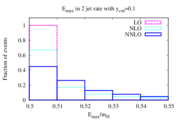
Figure 1: The energy spectrum of the leading jet in the decay H→b​b¯H\to b\bar{b} in the rest frame of the Higgs boson through NNLO. The jet clustering is performed with the JADE algorithm with yc​u​t=0.1y_{cut}=0.1.

In Fig. 1, we present the leading jet energy, Em​a​xE_{max}, in the rest frame of the Higgs boson, for events with two jets (yc​u​t=0.1y_{cut}=0.1). This is a new result which can only be obtained with a fully differential NNLO calculation and cannot be inferred from the inclusive decay width and NLO calculations. At leading order, Em​a​x=mH2E_{max}=\frac{m_{H}}{2}. At higher orders, there is a range of jet energies which are kinematically allowed. We choose a value of αs​(mZ)=0.118\alpha_{s}(m_{Z})=0.118 at the Z boson mass and evolve consistently through LO, NLO and NNLO up to the Higgs boson mass, which we assume to be mH=120​GeVm_{H}=120{\rm GeV}.

The above numerical results demonstrate the applicability of our method to physical processes. A number of phenomenological studies which are relevant to the searches of the Higgs boson can be made. It is easy to interface our numerical code with a Monte-Carlo code for the production of a Higgs boson. We we will present complete phenomenological studies pursuing this direction in the future.

8 Conclusions

In this paper, we present a first physical application of a new method for the factorization of overlapping singularities in phase space and loop integrations. We compute the fully differential decay width of a Higgs boson to a bottom-quark pair. We produce the required tree, one-loop and two-loop amplitudes with standard Feynman diagrammatic methods.

Our article focuses on the phase space integrations which emerge at NNLO. We apply non-linear mappings to factorize all overlapping singularities in all real-virtual and double-real integrations. Consequently, we perform the expansion of all integrals in the dimension regulator ϵ\epsilon with simple subtractions. The formalism allows for the computation of the decay rate for arbitrary physical observables.

We verify that we can reproduce the known results for the NNLO inclusive decay width and compute the differential two,three and four jet rates with the JADE algorithm. We also present the leading jet energy distributions, a new result that cannot be inferred from previous calculations. In the future, we will interface our NNLO Monte-Carlo to Monte-Carlo programs for the production of a Higgs boson.

We believe that our method for NNLO computations is powerful and suitable for complicated physical processes. We are looking forward to further apply our method on other interesting processes at hadron colliders.

9 Acknowledgements

We thank Andrea Banfi and Zoltan Kunszt for useful discussions. This research is supported by the ERC Starting Grant for the project “IterQCD” and the Swiss National Foundation under contract SNF 200020-126632.

Appendix A Double-real matrix elements

The function B⁡(p1,p2,p3,p4)B(p_{1},p_{2},p_{3},p_{4}) occurring in the H→b​b¯​b​b¯H\rightarrow b\bar{b}b\bar{b} squared amplitude can be expressed as

B⁡(p1,p2,p3,p4)\displaystyle B(p_{1},p_{2},p_{3},p_{4}) =\displaystyle= 2​s34−1−2​s134−1−4​s234−1+2​s124−1−2​s12​(s132+2​s122+2​s12​s13)s14​s34​s124​s234\displaystyle 2\,{s_{{34}}}^{-1}-2\,{s_{{134}}}^{-1}-4\,{s_{{234}}}^{-1}+2\,{s_{{124}}}^{-1}-2\,{\frac{s_{{12}}\left({s_{{13}}}^{2}+2\,{s_{{12}}}^{2}+2\,s_{{12}}s_{{13}}\right)}{s_{{14}}s_{{34}}s_{{124}}s_{{234}}}} (69)
+4​s12​s23s34​s134​s234−2​s12​(s23+2​s13+s12)s14​s34​s124+4​s12​s23s14​s124​s134+\displaystyle+4\,{\frac{s_{{12}}s_{{23}}}{s_{{34}}s_{{134}}s_{{234}}}}-2\,{\frac{s_{{12}}\left(s_{{23}}+2\,s_{{13}}+s_{{12}}\right)}{s_{{14}}s_{{34}}s_{{124}}}}+4\,{\frac{s_{{12}}s_{{23}}}{s_{{14}}s_{{124}}s_{{134}}}}+
(4​s13​s14+2​s132+4​s12​s13+2​s142+2​s12​s14s34​s124​s234+−2​s24−4​s13s14​s34CLOSE\displaystyle\Bigg({\frac{4\,s_{{13}}s_{{14}}+2\,{s_{{13}}}^{2}+4\,s_{{12}}s_{{13}}+2\,{s_{{14}}}^{2}+2\,s_{{12}}s_{{14}}}{s_{{34}}s_{{124}}s_{{234}}}}+{\frac{-2\,s_{{24}}-4\,s_{{13}}}{s_{{14}}s_{{34}}}}
+−2​s24+2​s12−2​s23s14​s234+4​s14−4​s23s124​s134+−4​s12−4​s14−4​s13s134​s234\displaystyle+{\frac{-2\,s_{{24}}+2\,s_{{12}}-2\,s_{{23}}}{s_{{14}}s_{{234}}}}+{\frac{4\,s_{{14}}-4\,s_{{23}}}{s_{{124}}s_{{134}}}}+{\frac{-4\,s_{{12}}-4\,s_{{14}}-4\,s_{{13}}}{s_{{134}}s_{{234}}}}
+2​s14+4​s13+2​s23s34​s124+2​s12​s13s14​s34​s124+−2​s24+2​s12s14​s124−2​s13​(−s23+s13)s14​s34​s234\displaystyle+{\frac{2\,s_{{14}}+4\,s_{{13}}+2\,s_{{23}}}{s_{{34}}s_{{124}}}}+2\,{\frac{s_{{12}}s_{{13}}}{s_{{14}}s_{{34}}s_{{124}}}}+{\frac{-2\,s_{{24}}+2\,s_{{12}}}{s_{{14}}s_{{124}}}}-2\,{\frac{s_{{13}}\left(-s_{{23}}+s_{{13}}\right)}{s_{{14}}s_{{34}}s_{{234}}}}
+−4​s13−2​s14+2​s23s34​s234+4​s12​s13+2​s24​s23+2​s242s14​s124​s234+−4​s12−4​s24−4​s23s1342\displaystyle+{\frac{-4\,s_{{13}}-2\,s_{{14}}+2\,s_{{23}}}{s_{{34}}s_{{234}}}}+{\frac{4\,s_{{12}}s_{{13}}+2\,s_{{24}}s_{{23}}+2\,{s_{{24}}}^{2}}{s_{{14}}s_{{124}}s_{{234}}}}+{\frac{-4\,s_{{12}}-4\,s_{{24}}-4\,s_{{23}}}{{s_{{134}}}^{2}}}
+2​s24+2​s23s34​s134+2​s14−1+2​s12​s132s14​s34​s124​s234−8​s134−1+2​s234−1+2​s12+2​s24s14​s134\displaystyle+{\frac{2\,s_{{24}}+2\,s_{{23}}}{s_{{34}}s_{{134}}}}+2\,{s_{{14}}}^{-1}+2\,{\frac{s_{{12}}{s_{{13}}}^{2}}{s_{{14}}s_{{34}}s_{{124}}s_{{234}}}}-8\,{s_{{134}}}^{-1}+2\,{s_{{234}}}^{-1}+{\frac{2\,s_{{12}}+2\,s_{{24}}}{s_{{14}}s_{{134}}}}
OPEN−2​s124−1)​ϵ2+(−4​s14−1+6​s34−1+6​s134−1+4​s234−1−2​s124−1CLOSE\displaystyle-2\,{s_{{124}}}^{-1}\Bigg){\epsilon}^{2}+\Bigg(-4\,{s_{{14}}}^{-1}+6\,{s_{{34}}}^{-1}+6\,{s_{{134}}}^{-1}+4\,{s_{{234}}}^{-1}-2\,{s_{{124}}}^{-1}
+2​s12​s132s14​s34​s124​s234−4​s12​s23s34​s134​s234−4​s12​s23s14​s124​s134\displaystyle+2\,{\frac{s_{{12}}{s_{{13}}}^{2}}{s_{{14}}s_{{34}}s_{{124}}s_{{234}}}}-4\,{\frac{s_{{12}}s_{{23}}}{s_{{34}}s_{{134}}s_{{234}}}}-4\,{\frac{s_{{12}}s_{{23}}}{s_{{14}}s_{{124}}s_{{134}}}}
−2​s12​(−s23−2​s13+s12)s14​s34​s124+4​s12+4​s24+4​s23s1342\displaystyle-2\,{\frac{s_{{12}}\left(-s_{{23}}-2\,s_{{13}}+s_{{12}}\right)}{s_{{14}}s_{{34}}s_{{124}}}}+{\frac{4\,s_{{12}}+4\,s_{{24}}+4\,s_{{23}}}{{s_{{134}}}^{2}}}
+−6​s24−8​s13s14​s34+−6​s12−2​s23+6​s34+8​s13s14​s134+6​s13+6​s24−2​s14+2​s23s34​s134\displaystyle+{\frac{-6\,s_{{24}}-8\,s_{{13}}}{s_{{14}}s_{{34}}}}+{\frac{-6\,s_{{12}}-2\,s_{{23}}+6\,s_{{34}}+8\,s_{{13}}}{s_{{14}}s_{{134}}}}+{\frac{6\,s_{{13}}+6\,s_{{24}}-2\,s_{{14}}+2\,s_{{23}}}{s_{{34}}s_{{134}}}}
+6​s13+4​s24+10​s12s14​s234+−2​s23−4​s24+2​s14+4​s12s34​s234+−4​s13−2​s14−4​s12s134​s234\displaystyle+{\frac{6\,s_{{13}}+4\,s_{{24}}+10\,s_{{12}}}{s_{{14}}s_{{234}}}}+{\frac{-2\,s_{{23}}-4\,s_{{24}}+2\,s_{{14}}+4\,s_{{12}}}{s_{{34}}s_{{234}}}}+{\frac{-4\,s_{{13}}-2\,s_{{14}}-4\,s_{{12}}}{s_{{134}}s_{{234}}}}
+−2​s24−2​s12s14​s124+6​s23−8​s12−8​s14+6​s13s34​s124+−2​s13−4​s23+2​s14s124​s134\displaystyle+{\frac{-2\,s_{{24}}-2\,s_{{12}}}{s_{{14}}s_{{124}}}}+{\frac{6\,s_{{23}}-8\,s_{{12}}-8\,s_{{14}}+6\,s_{{13}}}{s_{{34}}s_{{124}}}}+{\frac{-2\,s_{{13}}-4\,s_{{23}}+2\,s_{{14}}}{s_{{124}}s_{{134}}}}
+−4​s14−4​s13−8​s12s124​s234+4​s13​(s12+s24+s23)s14​s1342+4​s13​(s12+s24+s23)s34​s1342\displaystyle+{\frac{-4\,s_{{14}}-4\,s_{{13}}-8\,s_{{12}}}{s_{{124}}s_{{234}}}}+4\,{\frac{s_{{13}}\left(s_{{12}}+s_{{24}}+s_{{23}}\right)}{s_{{14}}{s_{{134}}}^{2}}}+4\,{\frac{s_{{13}}\left(s_{{12}}+s_{{24}}+s_{{23}}\right)}{s_{{34}}{s_{{134}}}^{2}}}
+4​s13​s23+2​s12​s23−2​s132−2​s232s14​s34​s234\displaystyle+{\frac{4\,s_{{13}}s_{{23}}+2\,s_{{12}}s_{{23}}-2\,{s_{{13}}}^{2}-2\,{s_{{23}}}^{2}}{s_{{14}}s_{{34}}s_{{234}}}}
+2​s122+4​s232+8​s24​s23+4​s12​s23+6​s242+8​s12​s24s14​s234​s134\displaystyle+{\frac{2\,{s_{{12}}}^{2}+4\,{s_{{23}}}^{2}+8\,s_{{24}}s_{{23}}+4\,s_{{12}}s_{{23}}+6\,{s_{{24}}}^{2}+8\,s_{{12}}s_{{24}}}{s_{{14}}s_{{234}}s_{{134}}}}
+−4​s12​s23+6​s142+4​s12​s14+2​s232+2​s122−8​s23​s14s34​s124​s134+2​s242+2​s24​s23−4​s122s14​s124​s234\displaystyle+{\frac{-4\,s_{{12}}s_{{23}}+6\,{s_{{14}}}^{2}+4\,s_{{12}}s_{{14}}+2\,{s_{{23}}}^{2}+2\,{s_{{12}}}^{2}-8\,s_{{23}}s_{{14}}}{s_{{34}}s_{{124}}s_{{134}}}}+{\frac{2\,{s_{{24}}}^{2}+2\,s_{{24}}s_{{23}}-4\,{s_{{12}}}^{2}}{s_{{14}}s_{{124}}s_{{234}}}}
OPEN+−4​s122−6​s12​s14+2​s132−2​s142s34​s124​s234)​ϵ+4​s12+4​s23+8​s13s14​s34\displaystyle+{\frac{-4\,{s_{{12}}}^{2}-6\,s_{{12}}s_{{14}}+2\,{s_{{13}}}^{2}-2\,{s_{{14}}}^{2}}{s_{{34}}s_{{124}}s_{{234}}}}\Bigg)\epsilon+{\frac{4\,s_{{12}}+4\,s_{{23}}+8\,s_{{13}}}{s_{{14}}s_{{34}}}}
+−6​s13−2​s14−4​s24s34​s134+2​s23−2​s24+4​s12−2​s34−4​s13s14​s134\displaystyle+{\frac{-6\,s_{{13}}-2\,s_{{14}}-4\,s_{{24}}}{s_{{34}}s_{{134}}}}+{\frac{2\,s_{{23}}-2\,s_{{24}}+4\,s_{{12}}-2\,s_{{34}}-4\,s_{{13}}}{s_{{14}}s_{{134}}}}
+−4​s23−10​s12+4​s24−6​s13s14​s234+4​s12+4​s13+2​s23+2​s14s34​s234\displaystyle+{\frac{-4\,s_{{23}}-10\,s_{{12}}+4\,s_{{24}}-6\,s_{{13}}}{s_{{14}}s_{{234}}}}+{\frac{4\,s_{{12}}+4\,s_{{13}}+2\,s_{{23}}+2\,s_{{14}}}{s_{{34}}s_{{234}}}}
+2​s14+4​s13+4​s12s134​s234+2​s12+2​s24s14​s124+−6​s13−6​s23−4​s12s34​s124+2​s13−2​s14+4​s23s124​s134\displaystyle+{\frac{2\,s_{{14}}+4\,s_{{13}}+4\,s_{{12}}}{s_{{134}}s_{{234}}}}+{\frac{2\,s_{{12}}+2\,s_{{24}}}{s_{{14}}s_{{124}}}}+{\frac{-6\,s_{{13}}-6\,s_{{23}}-4\,s_{{12}}}{s_{{34}}s_{{124}}}}+{\frac{2\,s_{{13}}-2\,s_{{14}}+4\,s_{{23}}}{s_{{124}}s_{{134}}}}
+4​s14+4​s13+8​s12s124​s234−4​s13​(s12+s24+s23)s14​s1342−4​s13​(s12+s24+s23)s34​s1342\displaystyle+{\frac{4\,s_{{14}}+4\,s_{{13}}+8\,s_{{12}}}{s_{{124}}s_{{234}}}}-4\,{\frac{s_{{13}}\left(s_{{12}}+s_{{24}}+s_{{23}}\right)}{s_{{14}}{s_{{134}}}^{2}}}-4\,{\frac{s_{{13}}\left(s_{{12}}+s_{{24}}+s_{{23}}\right)}{s_{{34}}{s_{{134}}}^{2}}}
+−2​s232−2​s12​s23+2​s132−4​s13​s23+4​s122+4​s242+4​s12​s13−4​s24​s13−4​s12​s24s14​s34​s234\displaystyle+{\frac{-2\,{s_{{23}}}^{2}-2\,s_{{12}}s_{{23}}+2\,{s_{{13}}}^{2}-4\,s_{{13}}s_{{23}}+4\,{s_{{12}}}^{2}+4\,{s_{{24}}}^{2}+4\,s_{{12}}s_{{13}}-4\,s_{{24}}s_{{13}}-4\,s_{{12}}s_{{24}}}{s_{{14}}s_{{34}}s_{{234}}}}
+−2​s122−2​s242−4​s232−4​s12​s24−4​s24​s23−4​s12​s23s14​s234​s134\displaystyle+{\frac{-2\,{s_{{12}}}^{2}-2\,{s_{{24}}}^{2}-4\,{s_{{23}}}^{2}-4\,s_{{12}}s_{{24}}-4\,s_{{24}}s_{{23}}-4\,s_{{12}}s_{{23}}}{s_{{14}}s_{{234}}s_{{134}}}}
+−2​s232−2​s122+4​s23​s14−2​s142s34​s124​s134+4​s122−2​s24​s23−2​s242s14​s124​s234\displaystyle+{\frac{-2\,{s_{{23}}}^{2}-2\,{s_{{12}}}^{2}+4\,s_{{23}}s_{{14}}-2\,{s_{{14}}}^{2}}{s_{{34}}s_{{124}}s_{{134}}}}+{\frac{4\,{s_{{12}}}^{2}-2\,s_{{24}}s_{{23}}-2\,{s_{{24}}}^{2}}{s_{{14}}s_{{124}}s_{{234}}}}
+−4​s13​s14−8​s122−2​s132−2​s142−8​s12​s13−6​s12​s14s34​s124​s234\displaystyle+{\frac{-4\,s_{{13}}s_{{14}}-8\,{s_{{12}}}^{2}-2\,{s_{{13}}}^{2}-2\,{s_{{14}}}^{2}-8\,s_{{12}}s_{{13}}-6\,s_{{12}}s_{{14}}}{s_{{34}}s_{{124}}s_{{234}}}}
AH​b​b¯​g​g(0)\displaystyle A^{(0)}_{Hb\bar{b}gg} =\displaystyle= 20​s234−1+20​s134−1+32​s13−1+24​s24−1+24​s14−1+32​s23−1\displaystyle 20\,{s_{234}}^{-1}+20\,{s_{134}}^{-1}+32\,{s_{{13}}}^{-1}+24\,{s_{{24}}}^{-1}+24\,{s_{{14}}}^{-1}+32\,{s_{{23}}}^{-1} (70)
+4​3​s13−6​mH2+3​s14+6​s34s24​s23+8​3​s24−6​mH2+3​s14+3​s34s13​s23\displaystyle+4\,{\frac{3\,s_{{13}}-6\,{m_{{H}}}^{2}+3\,s_{{14}}+6\,s_{{34}}}{s_{{24}}s_{{23}}}}+8\,{\frac{3\,s_{{24}}-6\,{m_{{H}}}^{2}+3\,s_{{14}}+3\,s_{{34}}}{s_{{13}}s_{{23}}}}
+4​6​mH2−3​s13+3​s34+3​s24s234​s14+4​−s24−s14+s34+4​mH2s234​s13\displaystyle+4\,{\frac{6\,{m_{{H}}}^{2}-3\,s_{{13}}+3\,s_{{34}}+3\,s_{{24}}}{s_{234}\,s_{{14}}}}+4\,{\frac{-s_{{24}}-s_{{14}}+s_{{34}}+4\,{m_{{H}}}^{2}}{s_{234}\,s_{{13}}}}
−4​−3​s14−6​mH2+3​s23−3​s34s134​s24+4​3​s23+6​s34−6​mH2+3​s24s13​s14\displaystyle-4\,{\frac{-3\,s_{{14}}-6\,{m_{{H}}}^{2}+3\,s_{{23}}-3\,s_{{34}}}{s_{134}\,s_{{24}}}}+4\,{\frac{3\,s_{{23}}+6\,s_{{34}}-6\,{m_{{H}}}^{2}+3\,s_{{24}}}{s_{{13}}s_{{14}}}}
+8​−5​s34−8​mH2−4​s24−4​s14s134​s234+8​mH2s1342+8​mH2s2342\displaystyle+8\,{\frac{-5\,s_{{34}}-8\,{m_{{H}}}^{2}-4\,s_{{24}}-4\,s_{{14}}}{s_{134}\,s_{234}}}+8\,{\frac{{m_{{H}}}^{2}}{{s_{134}}^{2}}}+8\,{\frac{{m_{{H}}}^{2}}{{s_{234}}^{2}}}
−4​8​mH2−5​s14−7​s34−5​s23s24​s13+4​−s24−s14+s34+4​mH2s134​s23\displaystyle-4\,{\frac{8\,{m_{{H}}}^{2}-5\,s_{{14}}-7\,s_{{34}}-5\,s_{{23}}}{s_{{24}}s_{{13}}}}+4\,{\frac{-s_{{24}}-s_{{14}}+s_{{34}}+4\,{m_{{H}}}^{2}}{s_{134}\,s_{{23}}}}
−4​−5​s24+8​mH2−5​s13−7​s34s14​s23−4​−s14−2​s34+s13−3​mH2s234​s24\displaystyle-4\,{\frac{-5\,s_{{24}}+8\,{m_{{H}}}^{2}-5\,s_{{13}}-7\,s_{{34}}}{s_{{14}}s_{{23}}}}-4\,{\frac{-s_{{14}}-2\,s_{{34}}+s_{{13}}-3\,{m_{{H}}}^{2}}{s_{234}\,s_{{24}}}}
+8​3​s23+3​s13+3​s34−6​mH2s24​s14−4​−3​mH2−2​s34−s24+s23s134​s14\displaystyle+8\,{\frac{3\,s_{{23}}+3\,s_{{13}}+3\,s_{{34}}-6\,{m_{{H}}}^{2}}{s_{{24}}s_{{14}}}}-4\,{\frac{-3\,{m_{{H}}}^{2}-2\,s_{{34}}-s_{{24}}+s_{{23}}}{s_{134}\,s_{{14}}}}
+4​(mH2+s34)​(−2​mH4−s342−2​mH2​s34)s234​s134​s13​s23\displaystyle+4\,{\frac{\left({m_{{H}}}^{2}+s_{{34}}\right)\left(-2\,{m_{{H}}}^{4}-{s_{{34}}}^{2}-2\,{m_{{H}}}^{2}s_{{34}}\right)}{s_{234}\,s_{134}\,s_{{13}}s_{{23}}}}
+4​(mH2+s34)​(−2​mH4−s342−2​mH2​s34)s234​s134​s14​s24\displaystyle+4\,{\frac{\left({m_{{H}}}^{2}+s_{{34}}\right)\left(-2\,{m_{{H}}}^{4}-{s_{{34}}}^{2}-2\,{m_{{H}}}^{2}s_{{34}}\right)}{s_{234}\,s_{134}\,s_{{14}}s_{{24}}}}
+4​(−s34+mH2)​(−2​mH4−s342+2​mH2​s34)s13​s14​s23​s24\displaystyle+4\,{\frac{\left(-s_{{34}}+{m_{{H}}}^{2}\right)\left(-2\,{m_{{H}}}^{4}-{s_{{34}}}^{2}+2\,{m_{{H}}}^{2}s_{{34}}\right)}{s_{{13}}s_{{14}}s_{{23}}s_{{24}}}}
−4​3​mH2​s13−s342−s132−4​mH4−3​mH2​s34+s13​s34s234​s24​s14\displaystyle-4\,{\frac{3\,{m_{{H}}}^{2}s_{{13}}-{s_{{34}}}^{2}-{s_{{13}}}^{2}-4\,{m_{{H}}}^{4}-3\,{m_{{H}}}^{2}s_{{34}}+s_{{13}}s_{{34}}}{s_{234}s_{24}s_{14}}}
−4​−s342−4​mH4−s242+s24​s34+3​mH2​s24−3​mH2​s34s134​s13​s23\displaystyle-4\,{\frac{-{s_{{34}}}^{2}-4\,{m_{{H}}}^{4}-{s_{{24}}}^{2}+s_{{24}}s_{{34}}+3\,{m_{{H}}}^{2}s_{{24}}-3\,{m_{{H}}}^{2}s_{{34}}}{s_{134}\,s_{{13}}s_{{23}}}}
−4​3​mH2​s14−s142+s14​s34−3​mH2​s34−4​mH4−s342s234​s13​s23\displaystyle-4\,{\frac{3\,{m_{{H}}}^{2}s_{{14}}-{s_{{14}}}^{2}+s_{{14}}s_{{34}}-3\,{m_{{H}}}^{2}s_{{34}}-4\,{m_{{H}}}^{4}-{s_{{34}}}^{2}}{s_{234}\,s_{{13}}s_{{23}}}}
−4​s23​s34−4​mH4−3​mH2​s34−s342−s232+3​mH2​s23s134​s14​s24\displaystyle-4\,{\frac{s_{{23}}s_{{34}}-4\,{m_{{H}}}^{4}-3\,{m_{{H}}}^{2}s_{{34}}-{s_{{34}}}^{2}-{s_{{23}}}^{2}+3\,{m_{{H}}}^{2}s_{{23}}}{s_{134}\,s_{{14}}s_{{24}}}}
+4​−s342−4​mH4−s242+s24​s34+3​mH2​s24−3​mH2​s34s134​s13​s234\displaystyle+4\,{\frac{-{s_{{34}}}^{2}-4\,{m_{{H}}}^{4}-{s_{{24}}}^{2}+s_{{24}}s_{{34}}+3\,{m_{{H}}}^{2}s_{{24}}-3\,{m_{{H}}}^{2}s_{{34}}}{s_{134}\,s_{{13}}s_{234}}}
+4​−s242−3​s24​s34−4​mH4−3​s342−6​mH2​s34−3​mH2​s24s234​s134​s14\displaystyle+4\,{\frac{-{s_{{24}}}^{2}-3\,s_{{24}}s_{{34}}-4\,{m_{{H}}}^{4}-3\,{s_{{34}}}^{2}-6\,{m_{{H}}}^{2}s_{{34}}-3\,{m_{{H}}}^{2}s_{{24}}}{s_{234}\,s_{134}\,s_{{14}}}}
+4​−3​s342−3​s14​s34−4​mH4−3​mH2​s14−s142−6​mH2​s34s134​s234​s24\displaystyle+4\,{\frac{-3\,{s_{{34}}}^{2}-3\,s_{{14}}s_{{34}}-4\,{m_{{H}}}^{4}-3\,{m_{{H}}}^{2}s_{{14}}-{s_{{14}}}^{2}-6\,{m_{{H}}}^{2}s_{{34}}}{s_{134}\,s_{234}\,s_{{24}}}}
+4​3​mH2​s14−s142+s14​s34−3​mH2​s34−4​mH4−s342s234​s134​s23\displaystyle+4\,{\frac{3\,{m_{{H}}}^{2}s_{{14}}-{s_{{14}}}^{2}+s_{{14}}s_{{34}}-3\,{m_{{H}}}^{2}s_{{34}}-4\,{m_{{H}}}^{4}-{s_{{34}}}^{2}}{s_{234}\,s_{134}\,s_{{23}}}}
+4​4​mH4+s232+3​s342−3​mH2​s23−6​mH2​s34+3​s23​s34s24​s13​s14\displaystyle+4\,{\frac{4\,{m_{{H}}}^{4}+{s_{{23}}}^{2}+3\,{s_{{34}}}^{2}-3\,{m_{{H}}}^{2}s_{{23}}-6\,{m_{{H}}}^{2}s_{{34}}+3\,s_{{23}}s_{{34}}}{s_{{24}}s_{{13}}s_{{14}}}}
+4​4​mH4+3​s342+s242−6​mH2​s34+3​s24​s34−3​mH2​s24s13​s14​s23\displaystyle+4\,{\frac{4\,{m_{{H}}}^{4}+3\,{s_{{34}}}^{2}+{s_{{24}}}^{2}-6\,{m_{{H}}}^{2}s_{{34}}+3\,s_{{24}}s_{{34}}-3\,{m_{{H}}}^{2}s_{{24}}}{s_{{13}}s_{{14}}s_{{23}}}}
+4​−3​mH2​s14+4​mH4+s142+3​s14​s34+3​s342−6​mH2​s34s24​s13​s23\displaystyle+4\,{\frac{-3\,{m_{{H}}}^{2}s_{{14}}+4\,{m_{{H}}}^{4}+{s_{{14}}}^{2}+3\,s_{{14}}s_{{34}}+3\,{s_{{34}}}^{2}-6\,{m_{{H}}}^{2}s_{{34}}}{s_{{24}}s_{{13}}s_{{23}}}}
+4​−6​mH2​s34+4​mH4+3​s13​s34+s132−3​mH2​s13+3​s342s24​s14​s23\displaystyle+4\,{\frac{-6\,{m_{{H}}}^{2}s_{{34}}+4\,{m_{{H}}}^{4}+3\,s_{{13}}s_{{34}}+{s_{{13}}}^{2}-3\,{m_{{H}}}^{2}s_{{13}}+3\,{s_{{34}}}^{2}}{s_{{24}}s_{{14}}s_{{23}}}}
AH​b​b¯​g​g(1)\displaystyle A^{(1)}_{Hb\bar{b}gg} =\displaystyle= −16​s234−1−32​s13−1−24​s14−1−16​s134−1−24​s24−1−32​s23−1\displaystyle-16\,{s_{{234}}}^{-1}-32\,{s_{{13}}}^{-1}-24\,{s_{{14}}}^{-1}-16\,{s_{{134}}}^{-1}-24\,{s_{{24}}}^{-1}-32\,{s_{{23}}}^{-1} (71)
−16​mH2s2342−16​mH2s1342−4​s14+2​s34s234​s24−4​s24+2​s34s134​s14\displaystyle-16\,{\frac{{m_{{H}}}^{2}}{{s_{{234}}}^{2}}}-16\,{\frac{{m_{{H}}}^{2}}{{s_{{134}}}^{2}}}-4\,{\frac{s_{{14}}+2\,s_{{34}}}{s_{{234}}s_{{24}}}}-4\,{\frac{s_{{24}}+2\,s_{{34}}}{s_{{134}}s_{{14}}}}
+8​−3​s24−3​s34+2​mH2−3​s14s13​s23+4​−5​s34−2​s13+mH2−2​s14s24​s23\displaystyle+8\,{\frac{-3\,s_{{24}}-3\,s_{{34}}+2\,{m_{{H}}}^{2}-3\,s_{{14}}}{s_{{13}}s_{{23}}}}+4\,{\frac{-5\,s_{{34}}-2\,s_{{13}}+{m_{{H}}}^{2}-2\,s_{{14}}}{s_{{24}}s_{{23}}}}
+4​−3​mH2−s34+s14+s24s134​s23+4​−3​s24−3​s34−3​mH2+4​s13s234​s14\displaystyle+4\,{\frac{-3\,{m_{{H}}}^{2}-s_{{34}}+s_{{14}}+s_{{24}}}{s_{{134}}s_{{23}}}}+4\,{\frac{-3\,s_{{24}}-3\,s_{{34}}-3\,{m_{{H}}}^{2}+4\,s_{{13}}}{s_{{234}}s_{{14}}}}
−4​−3​mH2+8​s34+6​s23+6​s14s24​s13−4​3​mH2+3​s34+3​s14−4​s23s134​s24\displaystyle-4\,{\frac{-3\,{m_{{H}}}^{2}+8\,s_{{34}}+6\,s_{{23}}+6\,s_{{14}}}{s_{{24}}s_{{13}}}}-4\,{\frac{3\,{m_{{H}}}^{2}+3\,s_{{34}}+3\,s_{{14}}-4\,s_{{23}}}{s_{{134}}s_{{24}}}}
+4​−3​mH2−s34+s14+s24s234​s13−4​−3​mH2+8​s34+6​s13+6​s24s14​s23\displaystyle+4\,{\frac{-3\,{m_{{H}}}^{2}-s_{{34}}+s_{{14}}+s_{{24}}}{s_{{234}}s_{{13}}}}-4\,{\frac{-3\,{m_{{H}}}^{2}+8\,s_{{34}}+6\,s_{{13}}+6\,s_{{24}}}{s_{{14}}s_{{23}}}}
+8​5​s34+4​mH2+4​s14+4​s24s134​s234−4​−mH2+s14s234​s23−4​−mH2+s24s134​s13\displaystyle+8\,{\frac{5\,s_{{34}}+4\,{m_{{H}}}^{2}+4\,s_{{14}}+4\,s_{{24}}}{s_{{134}}s_{{234}}}}-4\,{\frac{-{m_{{H}}}^{2}+s_{{14}}}{s_{{234}}s_{{23}}}}-4\,{\frac{-{m_{{H}}}^{2}+s_{{24}}}{s_{{134}}s_{{13}}}}
+8​2​mH2−3​s23−3​s13−3​s34s24​s14+4​−2​s24−5​s34−2​s23+mH2s13​s14\displaystyle+8\,{\frac{2\,{m_{{H}}}^{2}-3\,s_{{23}}-3\,s_{{13}}-3\,s_{{34}}}{s_{{24}}s_{{14}}}}+4\,{\frac{-2\,s_{{24}}-5\,s_{{34}}-2\,s_{{23}}+{m_{{H}}}^{2}}{s_{{13}}s_{{14}}}}
−4​s132−mH2​s13−s13​s34+mH2​s34+s342s234​s24​s14\displaystyle-4\,{\frac{{s_{{13}}}^{2}-{m_{{H}}}^{2}s_{{13}}-s_{{13}}s_{{34}}+{m_{{H}}}^{2}s_{{34}}+{s_{{34}}}^{2}}{s_{{234}}s_{{24}}s_{{14}}}}
−4​s242−mH2​s24−s24​s34+s342+mH2​s34s134​s13​s23\displaystyle-4\,{\frac{{s_{{24}}}^{2}-{m_{{H}}}^{2}s_{{24}}-s_{{24}}s_{{34}}+{s_{{34}}}^{2}+{m_{{H}}}^{2}s_{{34}}}{s_{{134}}s_{{13}}s_{{23}}}}
−4​−s14​s34+mH2​s34+s342−mH2​s14+s142s234​s13​s23\displaystyle-4\,{\frac{-s_{{14}}s_{{34}}+{m_{{H}}}^{2}s_{{34}}+{s_{{34}}}^{2}-{m_{{H}}}^{2}s_{{14}}+{s_{{14}}}^{2}}{s_{{234}}s_{{13}}s_{{23}}}}
−4​mH2​s34+s232−s23​s34−mH2​s23+s342s134​s14​s24\displaystyle-4\,{\frac{{m_{{H}}}^{2}s_{{34}}+{s_{{23}}}^{2}-s_{{23}}s_{{34}}-{m_{{H}}}^{2}s_{{23}}+{s_{{34}}}^{2}}{s_{{134}}s_{{14}}s_{{24}}}}
+4​−s14​s34+mH2​s34+s342−mH2​s14+s142s234​s134​s23\displaystyle+4\,{\frac{-s_{{14}}s_{{34}}+{m_{{H}}}^{2}s_{{34}}+{s_{{34}}}^{2}-{m_{{H}}}^{2}s_{{14}}+{s_{{14}}}^{2}}{s_{{234}}s_{{134}}s_{{23}}}}
+4​s242−mH2​s24−s24​s34+s342+mH2​s34s134​s13​s234\displaystyle+4\,{\frac{{s_{{24}}}^{2}-{m_{{H}}}^{2}s_{{24}}-s_{{24}}s_{{34}}+{s_{{34}}}^{2}+{m_{{H}}}^{2}s_{{34}}}{s_{{134}}s_{{13}}s_{{234}}}}
+4​s242+3​s342+mH2​s24+3​s24​s34+2​mH2​s34s234​s134​s14\displaystyle+4\,{\frac{{s_{{24}}}^{2}+3\,{s_{{34}}}^{2}+{m_{{H}}}^{2}s_{{24}}+3\,s_{{24}}s_{{34}}+2\,{m_{{H}}}^{2}s_{{34}}}{s_{{234}}s_{{134}}s_{{14}}}}
+4​2​mH2​s34+mH2​s14+s142+3​s342+3​s14​s34s134​s234​s24\displaystyle+4\,{\frac{2\,{m_{{H}}}^{2}s_{{34}}+{m_{{H}}}^{2}s_{{14}}+{s_{{14}}}^{2}+3\,{s_{{34}}}^{2}+3\,s_{{14}}s_{{34}}}{s_{{134}}s_{{234}}s_{{24}}}}
+4​−s132+2​mH2​s34+mH2​s13−3​s13​s34−3​s342s24​s14​s23\displaystyle+4\,{\frac{-{s_{{13}}}^{2}+2\,{m_{{H}}}^{2}s_{{34}}+{m_{{H}}}^{2}s_{{13}}-3\,s_{{13}}s_{{34}}-3\,{s_{{34}}}^{2}}{s_{{24}}s_{{14}}s_{{23}}}}
+4​−3​s23​s34+mH2​s23−s232−3​s342+2​mH2​s34s24​s13​s14\displaystyle+4\,{\frac{-3\,s_{{23}}s_{{34}}+{m_{{H}}}^{2}s_{{23}}-{s_{{23}}}^{2}-3\,{s_{{34}}}^{2}+2\,{m_{{H}}}^{2}s_{{34}}}{s_{{24}}s_{{13}}s_{{14}}}}
+4​mH2​s24+2​mH2​s34−3​s24​s34−s242−3​s342s13​s14​s23\displaystyle+4\,{\frac{{m_{{H}}}^{2}s_{{24}}+2\,{m_{{H}}}^{2}s_{{34}}-3\,s_{{24}}s_{{34}}-{s_{{24}}}^{2}-3\,{s_{{34}}}^{2}}{s_{{13}}s_{{14}}s_{{23}}}}
+4​−3​s342−s142+mH2​s14+2​mH2​s34−3​s14​s34s24​s13​s23\displaystyle+4\,{\frac{-3\,{s_{{34}}}^{2}-{s_{{14}}}^{2}+{m_{{H}}}^{2}s_{{14}}+2\,{m_{{H}}}^{2}s_{{34}}-3\,s_{{14}}s_{{34}}}{s_{{24}}s_{{13}}s_{{23}}}}
+4​(−s34+mH2)​s342s13​s14​s23​s24+4​(mH2+s34)​s342s234​s134​s13​s23+4​(mH2+s34)​s342s234​s134​s14​s24\displaystyle+4\,{\frac{\left(-s_{{34}}+{m_{{H}}}^{2}\right){s_{{34}}}^{2}}{s_{{13}}s_{{14}}s_{{23}}s_{{24}}}}+4\,{\frac{\left({m_{{H}}}^{2}+s_{{34}}\right){s_{{34}}}^{2}}{s_{{234}}s_{{134}}s_{{13}}s_{{23}}}}+4\,{\frac{\left({m_{{H}}}^{2}+s_{{34}}\right){s_{{34}}}^{2}}{s_{{234}}s_{{134}}s_{{14}}s_{{24}}}}
AH​b​b¯​g​g(2)\displaystyle A^{(2)}_{Hb\bar{b}gg} =\displaystyle= −4​s23−1−4​s13−1−8​s134−1−8​s234−1\displaystyle-4\,{s_{{23}}}^{-1}-4\,{s_{{13}}}^{-1}-8\,{s_{{134}}}^{-1}-8\,{s_{{234}}}^{-1} (72)
+8​mH2s1342+8​mH2s2342+8​2​mH2+2​s34s134​s234−4​s34+mH2−s23s134​s14\displaystyle+8\,{\frac{{m_{{H}}}^{2}}{{s_{{134}}}^{2}}}+8\,{\frac{{m_{{H}}}^{2}}{{s_{{234}}}^{2}}}+8\,{\frac{2\,{m_{{H}}}^{2}+2\,s_{{34}}}{s_{{134}}s_{{234}}}}-4\,{\frac{s_{{34}}+{m_{{H}}}^{2}-s_{{23}}}{s_{{134}}s_{{14}}}}
−4​s34−s13+mH2s234​s24+4​−2​s34+s13−s24s234​s14−4​3​s34+s14+s23s24​s13\displaystyle-4\,{\frac{s_{{34}}-s_{{13}}+{m_{{H}}}^{2}}{s_{{234}}s_{{24}}}}+4\,{\frac{-2\,s_{{34}}+s_{{13}}-s_{{24}}}{s_{{234}}s_{{14}}}}-4\,{\frac{3\,s_{{34}}+s_{{14}}+s_{{23}}}{s_{{24}}s_{{13}}}}
+4​s14+s24−s34s134​s23−4​s14+2​s34−s23s134​s24+4​s14+s24−s34s234​s13\displaystyle+4\,{\frac{s_{{14}}+s_{{24}}-s_{{34}}}{s_{{134}}s_{{23}}}}-4\,{\frac{s_{{14}}+2\,s_{{34}}-s_{{23}}}{s_{{134}}s_{{24}}}}+4\,{\frac{s_{{14}}+s_{{24}}-s_{{34}}}{s_{{234}}s_{{13}}}}
−4​s24+3​s34+s13s14​s23−4​mH2−s14s234​s23−4​mH2−s24s134​s13\displaystyle-4\,{\frac{s_{{24}}+3\,s_{{34}}+s_{{13}}}{s_{{14}}s_{{23}}}}-4\,{\frac{{m_{{H}}}^{2}-s_{{14}}}{s_{{234}}s_{{23}}}}-4\,{\frac{{m_{{H}}}^{2}-s_{{24}}}{s_{{134}}s_{{13}}}}
+4​−s13+mH2−3​s34−s14s24​s23+4​−s24−3​s34+mH2−s23s13​s14\displaystyle+4\,{\frac{-s_{{13}}+{m_{{H}}}^{2}-3\,s_{{34}}-s_{{14}}}{s_{{24}}s_{{23}}}}+4\,{\frac{-s_{{24}}-3\,s_{{34}}+{m_{{H}}}^{2}-s_{{23}}}{s_{{13}}s_{{14}}}}
−4​mH2​s34−s13​s34+s342s234​s24​s14−4​s342−s24​s34+mH2​s34s134​s13​s23\displaystyle-4\,{\frac{{m_{{H}}}^{2}s_{{34}}-s_{{13}}s_{{34}}+{s_{{34}}}^{2}}{s_{{234}}s_{{24}}s_{{14}}}}-4\,{\frac{{s_{{34}}}^{2}-s_{{24}}s_{{34}}+{m_{{H}}}^{2}s_{{34}}}{s_{{134}}s_{{13}}s_{{23}}}}
−4​s342+mH2​s34−s14​s34s234​s13​s23−4​−s23​s34+mH2​s34+s342s134​s14​s24\displaystyle-4\,{\frac{{s_{{34}}}^{2}+{m_{{H}}}^{2}s_{{34}}-s_{{14}}s_{{34}}}{s_{{234}}s_{{13}}s_{{23}}}}-4\,{\frac{-s_{{23}}s_{{34}}+{m_{{H}}}^{2}s_{{34}}+{s_{{34}}}^{2}}{s_{{134}}s_{{14}}s_{{24}}}}
+4​s342−s24​s34+mH2​s34s134​s13​s234+4​s24​s34+mH2​s34+2​s342s234​s134​s14\displaystyle+4\,{\frac{{s_{{34}}}^{2}-s_{{24}}s_{{34}}+{m_{{H}}}^{2}s_{{34}}}{s_{{134}}s_{{13}}s_{{234}}}}+4\,{\frac{s_{{24}}s_{{34}}+{m_{{H}}}^{2}s_{{34}}+2\,{s_{{34}}}^{2}}{s_{{234}}s_{{134}}s_{{14}}}}
+4​s14​s34+mH2​s34+2​s342s134​s234​s24+4​s342+mH2​s34−s14​s34s234​s134​s23\displaystyle+4\,{\frac{s_{{14}}s_{{34}}+{m_{{H}}}^{2}s_{{34}}+2\,{s_{{34}}}^{2}}{s_{{134}}s_{{234}}s_{{24}}}}+4\,{\frac{{s_{{34}}}^{2}+{m_{{H}}}^{2}s_{{34}}-s_{{14}}s_{{34}}}{s_{{234}}s_{{134}}s_{{23}}}}
+4​−2​s342−s23​s34+mH2​s34s24​s13​s14+4​−s24​s34+mH2​s34−2​s342s13​s14​s23\displaystyle+4\,{\frac{-2\,{s_{{34}}}^{2}-s_{{23}}s_{{34}}+{m_{{H}}}^{2}s_{{34}}}{s_{{24}}s_{{13}}s_{{14}}}}+4\,{\frac{-s_{{24}}s_{{34}}+{m_{{H}}}^{2}s_{{34}}-2\,{s_{{34}}}^{2}}{s_{{13}}s_{{14}}s_{{23}}}}
+4​−2​s342−s14​s34+mH2​s34s24​s13​s23+4​−2​s342−s13​s34+mH2​s34s24​s14​s23\displaystyle+4\,{\frac{-2\,{s_{{34}}}^{2}-s_{{14}}s_{{34}}+{m_{{H}}}^{2}s_{{34}}}{s_{{24}}s_{{13}}s_{{23}}}}+4\,{\frac{-2\,{s_{{34}}}^{2}-s_{{13}}s_{{34}}+{m_{{H}}}^{2}s_{{34}}}{s_{{24}}s_{{14}}s_{{23}}}}
+4​(−s34+mH2)​s342s13​s14​s23​s24+4​(mH2+s34)​s342s234​s134​s13​s23+4​(mH2+s34)​s342s234​s134​s14​s24\displaystyle+4\,{\frac{\left(-s_{{34}}+{m_{{H}}}^{2}\right){s_{{34}}}^{2}}{s_{{13}}s_{{14}}s_{{23}}s_{{24}}}}+4\,{\frac{\left({m_{{H}}}^{2}+s_{{34}}\right){s_{{34}}}^{2}}{s_{{234}}s_{{134}}s_{{13}}s_{{23}}}}+4\,{\frac{\left({m_{{H}}}^{2}+s_{{34}}\right){s_{{34}}}^{2}}{s_{{234}}s_{{134}}s_{{14}}s_{{24}}}}
BH​b​b¯​g​g(0)\displaystyle B^{(0)}_{Hb\bar{b}gg} =\displaystyle= 8​s14−1+16​s23−1+8​s24−1+16​s13−1+40​s134−1+40​s234−1\displaystyle 8\,{s_{{14}}}^{-1}+16\,{s_{{23}}}^{-1}+8\,{s_{{24}}}^{-1}+16\,{s_{{13}}}^{-1}+40\,{s_{{134}}}^{-1}+40\,{s_{{234}}}^{-1} (73)
+8​mH2​(−2​mH2+s34+s14)s234​s24​s13+8​mH2​(−2​mH2+s34+s24)s134​s14​s23\displaystyle+8\,{\frac{{m_{{H}}}^{2}\left(-2\,{m_{{H}}}^{2}+s_{{34}}+s_{{14}}\right)}{s_{{234}}s_{{24}}s_{{13}}}}+8\,{\frac{{m_{{H}}}^{2}\left(-2\,{m_{{H}}}^{2}+s_{{34}}+s_{{24}}\right)}{s_{{134}}s_{{14}}s_{{23}}}}
−8​mH2​(2​mH2−s13+s24)s234​s14​s23−8​mH2​(2​mH2+s14−s23)s134​s13​s24\displaystyle-8\,{\frac{{m_{{H}}}^{2}\left(2\,{m_{{H}}}^{2}-s_{{13}}+s_{{24}}\right)}{s_{{234}}s_{{14}}s_{{23}}}}-8\,{\frac{{m_{{H}}}^{2}\left(2\,{m_{{H}}}^{2}+s_{{14}}-s_{{23}}\right)}{s_{{134}}s_{{13}}s_{{24}}}}
+16​mH6s134​s13​s234​s24+16​mH6s234​s134​s14​s23+8​s14+2​mH2s234​s13+8​mH2s134​s13\displaystyle+16\,{\frac{{m_{{H}}}^{6}}{s_{{134}}s_{{13}}s_{{234}}s_{{24}}}}+16\,{\frac{{m_{{H}}}^{6}}{s_{{234}}s_{{134}}s_{{14}}s_{{23}}}}+8\,{\frac{s_{{14}}+2\,{m_{{H}}}^{2}}{s_{{234}}s_{{13}}}}+8\,{\frac{{m_{{H}}}^{2}}{s_{{134}}s_{{13}}}}
−8​−3​mH2+s23−s24−s34s134​s14+8​2​s13+s34+2​s24−mH2s14​s23\displaystyle-8\,{\frac{-3\,{m_{{H}}}^{2}+s_{{23}}-s_{{24}}-s_{{34}}}{s_{{134}}s_{{14}}}}+8\,{\frac{2\,s_{{13}}+s_{{34}}+2\,s_{{24}}-{m_{{H}}}^{2}}{s_{{14}}s_{{23}}}}
−8​s13−s34−3​mH2−s14s234​s24+8​mH2s234​s23−8​mH2​s24s23​s2342+8​mH2​s34s1342​s14\displaystyle-8\,{\frac{s_{{13}}-s_{{34}}-3\,{m_{{H}}}^{2}-s_{{14}}}{s_{{234}}s_{{24}}}}+8\,{\frac{{m_{{H}}}^{2}}{s_{{234}}s_{{23}}}}-8\,{\frac{{m_{{H}}}^{2}s_{{24}}}{s_{{23}}{s_{{234}}}^{2}}}+8\,{\frac{{m_{{H}}}^{2}s_{{34}}}{{s_{{134}}}^{2}s_{{14}}}}
+8​mH2​s34s2342​s24−8​mH2​s14s1342​s13+8​−s242−4​mH4+3​mH2​s24s134​s13​s234\displaystyle+8\,{\frac{{m_{{H}}}^{2}s_{{34}}}{{s_{{234}}}^{2}s_{{24}}}}-8\,{\frac{{m_{{H}}}^{2}s_{{14}}}{{s_{{134}}}^{2}s_{{13}}}}+8\,{\frac{-{s_{{24}}}^{2}-4\,{m_{{H}}}^{4}+3\,{m_{{H}}}^{2}s_{{24}}}{s_{{134}}s_{{13}}s_{{234}}}}
+8​−2​s24​s34−3​mH2​s34−4​mH4−s242−s342−3​mH2​s24s234​s134​s14\displaystyle+8\,{\frac{-2\,s_{{24}}s_{{34}}-3\,{m_{{H}}}^{2}s_{{34}}-4\,{m_{{H}}}^{4}-{s_{{24}}}^{2}-{s_{{34}}}^{2}-3\,{m_{{H}}}^{2}s_{{24}}}{s_{{234}}s_{{134}}s_{{14}}}}
+8​−3​mH2​s34−s142−2​s14​s34−s342−4​mH4−3​mH2​s14s134​s234​s24\displaystyle+8\,{\frac{-3\,{m_{{H}}}^{2}s_{{34}}-{s_{{14}}}^{2}-2\,s_{{14}}s_{{34}}-{s_{{34}}}^{2}-4\,{m_{{H}}}^{4}-3\,{m_{{H}}}^{2}s_{{14}}}{s_{{134}}s_{{234}}s_{{24}}}}
+8​3​mH2​s14−4​mH4−s142s234​s134​s23+24​mH2s1342+24​mH2s2342\displaystyle+8\,{\frac{3\,{m_{{H}}}^{2}s_{{14}}-4\,{m_{{H}}}^{4}-{s_{{14}}}^{2}}{s_{{234}}s_{{134}}s_{{23}}}}+24\,{\frac{{m_{{H}}}^{2}}{{s_{{134}}}^{2}}}+24\,{\frac{{m_{{H}}}^{2}}{{s_{{234}}}^{2}}}
−8​−s34+s13−3​mH2−2​s24s234​s14+8​−mH2+s34+2​s14+2​s23s24​s13\displaystyle-8\,{\frac{-s_{{34}}+s_{{13}}-3\,{m_{{H}}}^{2}-2\,s_{{24}}}{s_{{234}}s_{{14}}}}+8\,{\frac{-{m_{{H}}}^{2}+s_{{34}}+2\,s_{{14}}+2\,s_{{23}}}{s_{{24}}s_{{13}}}}
+8​s24+2​mH2s134​s23−8​−s34−2​s14−3​mH2+s23s134​s24\displaystyle+8\,{\frac{s_{{24}}+2\,{m_{{H}}}^{2}}{s_{{134}}s_{{23}}}}-8\,{\frac{-s_{{34}}-2\,s_{{14}}-3\,{m_{{H}}}^{2}+s_{{23}}}{s_{{134}}s_{{24}}}}
+16​−6​mH2−4​s24−4​s14−3​s34s134​s234\displaystyle+16\,{\frac{-6\,{m_{{H}}}^{2}-4\,s_{{24}}-4\,s_{{14}}-3\,s_{{34}}}{s_{{134}}s_{{234}}}}
BH​b​b¯​g​g(1)\displaystyle B^{(1)}_{Hb\bar{b}gg} =\displaystyle= −8​s14−1−16​s23−1−8​s24−1−16​s13−1−48​s134−1−48​s234−1\displaystyle-8\,{s_{{14}}}^{-1}-16\,{s_{{23}}}^{-1}-8\,{s_{{24}}}^{-1}-16\,{s_{{13}}}^{-1}-48\,{s_{{134}}}^{-1}-48\,{s_{{234}}}^{-1} (74)
+8​mH2​(−2​s34−s14)s234​s24​s13+8​mH2​(−2​s34−s24)s134​s14​s23−8​mH2​(s13−2​s24)s234​s14​s23\displaystyle+8\,{\frac{{m_{{H}}}^{2}\left(-2\,s_{{34}}-s_{{14}}\right)}{s_{{234}}s_{{24}}s_{{13}}}}+8\,{\frac{{m_{{H}}}^{2}\left(-2\,s_{{34}}-s_{{24}}\right)}{s_{{134}}s_{{14}}s_{{23}}}}-8\,{\frac{{m_{{H}}}^{2}\left(s_{{13}}-2\,s_{{24}}\right)}{s_{{234}}s_{{14}}s_{{23}}}}
−8​mH2​(−2​s14+s23)s134​s13​s24+8​s13s234​s23−8​−mH2+s34−s23s134​s14\displaystyle-8\,{\frac{{m_{{H}}}^{2}\left(-2\,s_{{14}}+s_{{23}}\right)}{s_{{134}}s_{{13}}s_{{24}}}}+8\,{\frac{s_{{13}}}{s_{{234}}s_{{23}}}}-8\,{\frac{-{m_{{H}}}^{2}+s_{{34}}-s_{{23}}}{s_{{134}}s_{{14}}}}
−8​−s13−mH2+s34s234​s24+16​mH2​s24s23​s2342−16​mH2​s34s1342​s14\displaystyle-8\,{\frac{-s_{{13}}-{m_{{H}}}^{2}+s_{{34}}}{s_{{234}}s_{{24}}}}+16\,{\frac{{m_{{H}}}^{2}s_{{24}}}{s_{{23}}{s_{{234}}}^{2}}}-16\,{\frac{{m_{{H}}}^{2}s_{{34}}}{{s_{{134}}}^{2}s_{{14}}}}
−16​mH2​s34s2342​s24+16​mH2​s14s1342​s13−32​mH2s1342−32​mH2s2342\displaystyle-16\,{\frac{{m_{{H}}}^{2}s_{{34}}}{{s_{{234}}}^{2}s_{{24}}}}+16\,{\frac{{m_{{H}}}^{2}s_{{14}}}{{s_{{134}}}^{2}s_{{13}}}}-32\,{\frac{{m_{{H}}}^{2}}{{s_{{134}}}^{2}}}-32\,{\frac{{m_{{H}}}^{2}}{{s_{{234}}}^{2}}}
+8​s242−mH2​s24s134​s13​s234+8​2​s24​s34+s342+s242+mH2​s24+mH2​s34s234​s134​s14\displaystyle+8\,{\frac{{s_{{24}}}^{2}-{m_{{H}}}^{2}s_{{24}}}{s_{{134}}s_{{13}}s_{{234}}}}+8\,{\frac{2\,s_{{24}}s_{{34}}+{s_{{34}}}^{2}+{s_{{24}}}^{2}+{m_{{H}}}^{2}s_{{24}}+{m_{{H}}}^{2}s_{{34}}}{s_{{234}}s_{{134}}s_{{14}}}}
+8​s342+2​s14​s34+mH2​s14+s142+mH2​s34s134​s234​s24+8​s142−mH2​s14s234​s134​s23\displaystyle+8\,{\frac{{s_{{34}}}^{2}+2\,s_{{14}}s_{{34}}+{m_{{H}}}^{2}s_{{14}}+{s_{{14}}}^{2}+{m_{{H}}}^{2}s_{{34}}}{s_{{134}}s_{{234}}s_{{24}}}}+8\,{\frac{{s_{{14}}}^{2}-{m_{{H}}}^{2}s_{{14}}}{s_{{234}}s_{{134}}s_{{23}}}}
−8​−s13+mH2+2​s24+s34s234​s14+8​−2​s14+mH2−s34−2​s23s24​s13\displaystyle-8\,{\frac{-s_{{13}}+{m_{{H}}}^{2}+2\,s_{{24}}+s_{{34}}}{s_{{234}}s_{{14}}}}+8\,{\frac{-2\,s_{{14}}+{m_{{H}}}^{2}-s_{{34}}-2\,s_{{23}}}{s_{{24}}s_{{13}}}}
+8​−2​s24−3​mH2s134​s23+8​s23s134​s13−8​mH2−s23+s34+2​s14s134​s24\displaystyle+8\,{\frac{-2\,s_{{24}}-3\,{m_{{H}}}^{2}}{s_{{134}}s_{{23}}}}+8\,{\frac{s_{{23}}}{s_{{134}}s_{{13}}}}-8\,{\frac{{m_{{H}}}^{2}-s_{{23}}+s_{{34}}+2\,s_{{14}}}{s_{{134}}s_{{24}}}}
+8​−3​mH2−2​s14s234​s13+8​−s34−2​s24−2​s13+mH2s14​s23\displaystyle+8\,{\frac{-3\,{m_{{H}}}^{2}-2\,s_{{14}}}{s_{{234}}s_{{13}}}}+8\,{\frac{-s_{{34}}-2\,s_{{24}}-2\,s_{{13}}+{m_{{H}}}^{2}}{s_{{14}}s_{{23}}}}
+16​4​s14+4​s24+2​mH2+3​s34s134​s234\displaystyle+16\,{\frac{4\,s_{{14}}+4\,s_{{24}}+2\,{m_{{H}}}^{2}+3\,s_{{34}}}{s_{{134}}s_{{234}}}}
BH​b​b¯​g​g(2)\displaystyle B^{(2)}_{Hb\bar{b}gg} =\displaystyle= −8​s34+s24s134​s14−8​s23−1−8​s13−1−16​s134−1−16​s234−1\displaystyle-8\,{\frac{s_{{34}}+s_{{24}}}{s_{{134}}s_{{14}}}}-8\,{s_{{23}}}^{-1}-8\,{s_{{13}}}^{-1}-16\,{s_{{134}}}^{-1}-16\,{s_{{234}}}^{-1} (75)
+8​mH2​s34s234​s24​s13+8​mH2​s34s134​s14​s23−8​mH2​s24s234​s14​s23−8​mH2​s14s134​s13​s24\displaystyle+8\,{\frac{{m_{{H}}}^{2}s_{{34}}}{s_{{234}}s_{{24}}s_{{13}}}}+8\,{\frac{{m_{{H}}}^{2}s_{{34}}}{s_{{134}}s_{{14}}s_{{23}}}}-8\,{\frac{{m_{{H}}}^{2}s_{{24}}}{s_{{234}}s_{{14}}s_{{23}}}}-8\,{\frac{{m_{{H}}}^{2}s_{{14}}}{s_{{134}}s_{{13}}s_{{24}}}}
+8​−s13+mH2s234​s23−8​s34+s14s234​s24−8​mH2​s24s23​s2342\displaystyle+8\,{\frac{-s_{{13}}+{m_{{H}}}^{2}}{s_{{234}}s_{{23}}}}-8\,{\frac{s_{{34}}+s_{{14}}}{s_{{234}}s_{{24}}}}-8\,{\frac{{m_{{H}}}^{2}s_{{24}}}{s_{{23}}{s_{{234}}}^{2}}}
+8​mH2​s34s1342​s14+8​mH2​s34s2342​s24−8​mH2​s14s1342​s13\displaystyle+8\,{\frac{{m_{{H}}}^{2}s_{{34}}}{{s_{{134}}}^{2}s_{{14}}}}+8\,{\frac{{m_{{H}}}^{2}s_{{34}}}{{s_{{234}}}^{2}s_{{24}}}}-8\,{\frac{{m_{{H}}}^{2}s_{{14}}}{{s_{{134}}}^{2}s_{{13}}}}
+8​−s24​s34+mH2​s34s134​s13​s234+8​s342+s24​s34+mH2​s34s234​s134​s14\displaystyle+8\,{\frac{-s_{{24}}s_{{34}}+{m_{{H}}}^{2}s_{{34}}}{s_{{134}}s_{{13}}s_{{234}}}}+8\,{\frac{{s_{{34}}}^{2}+s_{{24}}s_{{34}}+{m_{{H}}}^{2}s_{{34}}}{s_{{234}}s_{{134}}s_{{14}}}}
+8​s342+mH2​s34+s14​s34s134​s234​s24+8​−s14​s34+mH2​s34s234​s134​s23\displaystyle+8\,{\frac{{s_{{34}}}^{2}+{m_{{H}}}^{2}s_{{34}}+s_{{14}}s_{{34}}}{s_{{134}}s_{{234}}s_{{24}}}}+8\,{\frac{-s_{{14}}s_{{34}}+{m_{{H}}}^{2}s_{{34}}}{s_{{234}}s_{{134}}s_{{23}}}}
+8​mH2s1342+8​mH2s2342−8​s34+mH2+s24−s13s234​s14\displaystyle+8\,{\frac{{m_{{H}}}^{2}}{{s_{{134}}}^{2}}}+8\,{\frac{{m_{{H}}}^{2}}{{s_{{234}}}^{2}}}-8\,{\frac{s_{{34}}+{m_{{H}}}^{2}+s_{{24}}-s_{{13}}}{s_{{234}}s_{{14}}}}
+8​−s23−s14−s34+mH2s24​s13+8​s24+s14s134​s23+8​−s23+mH2s134​s13\displaystyle+8\,{\frac{-s_{{23}}-s_{{14}}-s_{{34}}+{m_{{H}}}^{2}}{s_{{24}}s_{{13}}}}+8\,{\frac{s_{{24}}+s_{{14}}}{s_{{134}}s_{{23}}}}+8\,{\frac{-s_{{23}}+{m_{{H}}}^{2}}{s_{{134}}s_{{13}}}}
−8​mH2+s34−s23+s14s134​s24+8​s24+s14s234​s13\displaystyle-8\,{\frac{{m_{{H}}}^{2}+s_{{34}}-s_{{23}}+s_{{14}}}{s_{{134}}s_{{24}}}}+8\,{\frac{s_{{24}}+s_{{14}}}{s_{{234}}s_{{13}}}}
+8​mH2−s34−s13−s24s14​s23+16​2​mH2+2​s34s134​s234\displaystyle+8\,{\frac{{m_{{H}}}^{2}-s_{{34}}-s_{{13}}-s_{{24}}}{s_{{14}}s_{{23}}}}+16\,{\frac{2\,{m_{{H}}}^{2}+2\,s_{{34}}}{s_{{134}}s_{{234}}}}
CH​b​b¯​g​g(0)\displaystyle C^{(0)}_{Hb\bar{b}gg} =\displaystyle= 8​2​s24+4​mH2+s14−s13s234​s34−4​−s14−2​s13+4​mH2−4​s23s24​s34\displaystyle 8\,{\frac{2\,s_{{24}}+4\,{m_{{H}}}^{2}+s_{{14}}-s_{{13}}}{s_{{234}}s_{{34}}}}-4\,{\frac{-s_{{14}}-2\,s_{{13}}+4\,{m_{{H}}}^{2}-4\,s_{{23}}}{s_{{24}}s_{{34}}}} (76)
−4​−2​s14−2​s23+2​mH2−s24s13​s34−4​2​mH2−2​s13−s14−2​s24s23​s34\displaystyle-4\,{\frac{-2\,s_{{14}}-2\,s_{{23}}+2\,{m_{{H}}}^{2}-s_{{24}}}{s_{{13}}s_{{34}}}}-4\,{\frac{2\,{m_{{H}}}^{2}-2\,s_{{13}}-s_{{14}}-2\,s_{{24}}}{s_{{23}}s_{{34}}}}
+16​−mH2​s24−4​mH4−2​s24​s14−s142−s242−mH2​s14s134​s34​s234\displaystyle+16\,{\frac{-{m_{{H}}}^{2}s_{{24}}-4\,{m_{{H}}}^{4}-2\,s_{{24}}s_{{14}}-{s_{{14}}}^{2}-{s_{{24}}}^{2}-{m_{{H}}}^{2}s_{{14}}}{s_{{134}}s_{{34}}s_{{234}}}}
−4​−s242+2​mH2​s24−2​mH4−s142+2​mH2​s14−2​s24​s14s234​s34​s13\displaystyle-4\,{\frac{-{s_{{24}}}^{2}+2\,{m_{{H}}}^{2}s_{{24}}-2\,{m_{{H}}}^{4}-{s_{{14}}}^{2}+2\,{m_{{H}}}^{2}s_{{14}}-2\,s_{{24}}s_{{14}}}{s_{{234}}s_{{34}}s_{{13}}}}
−4​2​s24​s13−2​mH4−s242−s132+2​mH2​s13−2​mH2​s24s234​s34​s14\displaystyle-4\,{\frac{2\,s_{{24}}s_{{13}}-2\,{m_{{H}}}^{4}-{s_{{24}}}^{2}-{s_{{13}}}^{2}+2\,{m_{{H}}}^{2}s_{{13}}-2\,{m_{{H}}}^{2}s_{{24}}}{s_{{234}}s_{{34}}s_{{14}}}}
−32​s24​s14​mH2s134​s342​s234−4​−s24−2​s23+4​mH2−4​s13s14​s34\displaystyle-32\,{\frac{s_{{24}}s_{{14}}{m_{{H}}}^{2}}{s_{{134}}{s_{{34}}}^{2}s_{{234}}}}-4\,{\frac{-s_{{24}}-2\,s_{{23}}+4\,{m_{{H}}}^{2}-4\,s_{{13}}}{s_{{14}}s_{{34}}}}
−4​2​s14​s23−s232+2​mH2​s23−2​mH4−s142−2​mH2​s14s134​s34​s24\displaystyle-4\,{\frac{2\,s_{{14}}s_{{23}}-{s_{{23}}}^{2}+2\,{m_{{H}}}^{2}s_{{23}}-2\,{m_{{H}}}^{4}-{s_{{14}}}^{2}-2\,{m_{{H}}}^{2}s_{{14}}}{s_{{134}}s_{{34}}s_{{24}}}}
−8​−s24−4​mH2−2​s14+s23s134​s34+16​mH2​s24s2342​s34\displaystyle-8\,{\frac{-s_{{24}}-4\,{m_{{H}}}^{2}-2\,s_{{14}}+s_{{23}}}{s_{{134}}s_{{34}}}}+16\,{\frac{{m_{{H}}}^{2}s_{{24}}}{{s_{{234}}}^{2}s_{{34}}}}
−4​2​mH2​s24+2​mH2​s13−2​mH4−s242−2​s24​s13−s132s14​s23​s34\displaystyle-4\,{\frac{2\,{m_{{H}}}^{2}s_{{24}}+2\,{m_{{H}}}^{2}s_{{13}}-2\,{m_{{H}}}^{4}-{s_{{24}}}^{2}-2\,s_{{24}}s_{{13}}-{s_{{13}}}^{2}}{s_{{14}}s_{{23}}s_{{34}}}}
+16​s242​mH2s342​s2342+16​mH2​s14s1342​s34+16​s142​mH2s342​s1342\displaystyle+16\,{\frac{{s_{{24}}}^{2}{m_{{H}}}^{2}}{{s_{{34}}}^{2}{s_{{234}}}^{2}}}+16\,{\frac{{m_{{H}}}^{2}s_{{14}}}{{s_{{134}}}^{2}s_{{34}}}}+16\,{\frac{{s_{{14}}}^{2}{m_{{H}}}^{2}}{{s_{{34}}}^{2}{s_{{134}}}^{2}}}
−4​−2​s14​s23+2​mH2​s23−2​mH4−s232+2​mH2​s14−s142s24​s13​s34\displaystyle-4\,{\frac{-2\,s_{{14}}s_{{23}}+2\,{m_{{H}}}^{2}s_{{23}}-2\,{m_{{H}}}^{4}-{s_{{23}}}^{2}+2\,{m_{{H}}}^{2}s_{{14}}-{s_{{14}}}^{2}}{s_{{24}}s_{{13}}s_{{34}}}}
−4​−s242+2​mH2​s24−2​mH4−s142+2​mH2​s14−2​s24​s14s134​s34​s23\displaystyle-4\,{\frac{-{s_{{24}}}^{2}+2\,{m_{{H}}}^{2}s_{{24}}-2\,{m_{{H}}}^{4}-{s_{{14}}}^{2}+2\,{m_{{H}}}^{2}s_{{14}}-2\,s_{{24}}s_{{14}}}{s_{{134}}s_{{34}}s_{{23}}}}
CH​b​b¯​g​g(1)\displaystyle C^{(1)}_{Hb\bar{b}gg} =\displaystyle= 8​−s14−2​s24+s13s234​s34−4​s24+2​s23+s14s13​s34−4​s14+s24+2​s13s23​s34\displaystyle 8\,{\frac{-s_{{14}}-2\,s_{{24}}+s_{{13}}}{s_{{234}}s_{{34}}}}-4\,{\frac{s_{{24}}+2\,s_{{23}}+s_{{14}}}{s_{{13}}s_{{34}}}}-4\,{\frac{s_{{14}}+s_{{24}}+2\,s_{{13}}}{s_{{23}}s_{{34}}}} (77)
+32​s24​s14​mH2s134​s342​s234−4​2​s23+4​s13+s24s14​s34−4​−3​s14​s23+s232+s142s134​s34​s24\displaystyle+32\,{\frac{s_{{24}}s_{{14}}{m_{{H}}}^{2}}{s_{{134}}{s_{{34}}}^{2}s_{{234}}}}-4\,{\frac{2\,s_{{23}}+4\,s_{{13}}+s_{{24}}}{s_{{14}}s_{{34}}}}-4\,{\frac{-3\,s_{{14}}s_{{23}}+{s_{{23}}}^{2}+{s_{{14}}}^{2}}{s_{{134}}s_{{34}}s_{{24}}}}
−8​2​s14+s24−s23s134​s34−16​mH2​s24s2342​s34−4​3​s24​s13+s132+s242s14​s23​s34\displaystyle-8\,{\frac{2\,s_{{14}}+s_{{24}}-s_{{23}}}{s_{{134}}s_{{34}}}}-16\,{\frac{{m_{{H}}}^{2}s_{{24}}}{{s_{{234}}}^{2}s_{{34}}}}-4\,{\frac{3\,s_{{24}}s_{{13}}+{s_{{13}}}^{2}+{s_{{24}}}^{2}}{s_{{14}}s_{{23}}s_{{34}}}}
−16​s242​mH2s342​s2342−4​4​s23+s14+2​s13s24​s34−16​mH2​s14s1342​s34\displaystyle-16\,{\frac{{s_{{24}}}^{2}{m_{{H}}}^{2}}{{s_{{34}}}^{2}{s_{{234}}}^{2}}}-4\,{\frac{4\,s_{{23}}+s_{{14}}+2\,s_{{13}}}{s_{{24}}s_{{34}}}}-16\,{\frac{{m_{{H}}}^{2}s_{{14}}}{{s_{{134}}}^{2}s_{{34}}}}
+16​mH2​s14+2​s24​s14+mH2​s24+s142+s242s134​s34​s234−16​s142​mH2s342​s1342\displaystyle+16\,{\frac{{m_{{H}}}^{2}s_{{14}}+2\,s_{{24}}s_{{14}}+{m_{{H}}}^{2}s_{{24}}+{s_{{14}}}^{2}+{s_{{24}}}^{2}}{s_{{134}}s_{{34}}s_{{234}}}}-16\,{\frac{{s_{{14}}}^{2}{m_{{H}}}^{2}}{{s_{{34}}}^{2}{s_{{134}}}^{2}}}
−4​s242+s142+3​s24​s14s234​s34​s13−4​s242+s142+3​s24​s14s134​s34​s23\displaystyle-4\,{\frac{{s_{{24}}}^{2}+{s_{{14}}}^{2}+3\,s_{{24}}s_{{14}}}{s_{{234}}s_{{34}}s_{{13}}}}-4\,{\frac{{s_{{24}}}^{2}+{s_{{14}}}^{2}+3\,s_{{24}}s_{{14}}}{s_{{134}}s_{{34}}s_{{23}}}}
−4​s142+3​s14​s23+s232s24​s13​s34−4​s132+s242−3​s24​s13s234​s34​s14\displaystyle-4\,{\frac{{s_{{14}}}^{2}+3\,s_{{14}}s_{{23}}+{s_{{23}}}^{2}}{s_{{24}}s_{{13}}s_{{34}}}}-4\,{\frac{{s_{{13}}}^{2}+{s_{{24}}}^{2}-3\,s_{{24}}s_{{13}}}{s_{{234}}s_{{34}}s_{{14}}}}

References

  • [1] P. A. Baikov, K. G. Chetyrkin, J. H. Kuhn, Phys. Rev. Lett. 96 (2006) 012003. [hep-ph/0511063].
  • [2] S. G. Gorishnii, A. L. Kataev, S. A. Larin, Sov. J. Nucl. Phys. 40 (1984) 329-334.
  • [3] S. G. Gorishnii, A. L. Kataev, S. A. Larin, L. R. Surguladze, Mod. Phys. Lett. A5 (1990) 2703-2712.
  • [4] S. G. Gorishnii, A. L. Kataev, S. A. Larin, L. R. Surguladze, Phys. Rev. D43 (1991) 1633-1640.
  • [5] C. Becchi, S. Narison, E. de Rafael, F. J. Yndurain, Z. Phys. C8 (1981) 335.
  • [6] N. Sakai, Phys. Rev. D22 (1980) 2220.
  • [7] T. Inami, T. Kubota, Nucl. Phys. B179 (1981) 171.
  • [8] K. G. Chetyrkin, Phys. Lett. B390 (1997) 309-317. [hep-ph/9608318].
  • [9] K. G. Chetyrkin and M. Steinhauser, Phys. Lett. B 408 (1997) 320 [hep-ph/9706462].
  • [10] J. M. Butterworth, A. R. Davison, M. Rubin, G. P. Salam, Phys. Rev. Lett. 100 (2008) 242001. [arXiv:0802.2470 [hep-ph]].
  • [11] T. Plehn, G. P. Salam, M. Spannowsky, Phys. Rev. Lett. 104 (2010) 111801. [arXiv:0910.5472 [hep-ph]].
  • [12] ATLAS Collaboration, Atlas sensitivity to the standard model higgs in the HW and HZ channels at high transverse momenta, 2009. ATL-PHYS-PUB-2009-088.
  • [13] D. E. Soper and M. Spannowsky, JHEP 1008 (2010) 029 [arXiv:1005.0417 [hep-ph]].
  • [14] A. Bredenstein, A. Denner, S. Dittmaier, S. Pozzorini, JHEP 1003 (2010) 021. [arXiv:1001.4006 [hep-ph]].
  • [15] A. Denner, S. Dittmaier, S. Kallweit, S. Pozzorini, Phys. Rev. Lett. 106 (2011) 052001. [arXiv:1012.3975 [hep-ph]].
  • [16] T. Melia, K. Melnikov, R. Rontsch, G. Zanderighi, JHEP 1012 (2010) 053. [arXiv:1007.5313 [hep-ph]].
  • [17] R. K. Ellis, K. Melnikov, G. Zanderighi, Phys. Rev. D80 (2009) 094002. [arXiv:0906.1445 [hep-ph]].
  • [18] C. F. Berger, Z. Bern, L. J. Dixon, F. Febres Cordero, D. Forde, T. Gleisberg, H. Ita, D. A. Kosower et al., Phys. Rev. Lett. 106 (2011) 092001. [arXiv:1009.2338 [hep-ph]].
  • [19] C. F. Berger, Z. Bern, L. J. Dixon, F. Febres Cordero, D. Forde, T. Gleisberg, H. Ita, D. A. Kosower et al., Phys. Rev. D82 (2010) 074002. [arXiv:1004.1659 [hep-ph]].
  • [20] C. F. Berger, Z. Bern, L. J. Dixon, F. Febres Cordero, D. Forde, T. Gleisberg, H. Ita, D. A. Kosower et al., Phys. Rev. D80 (2009) 074036. [arXiv:0907.1984 [hep-ph]].
  • [21] H. Ita, Z. Bern, L. J. Dixon, F. F. Cordero, D. A. Kosower, D. Maitre, [arXiv:1108.2229 [hep-ph]].
  • [22] G. Bevilacqua, M. Czakon, C. G. Papadopoulos, R. Pittau, M. Worek, JHEP 0909 (2009) 109. [arXiv:0907.4723 [hep-ph]].
  • [23] G. Bevilacqua, M. Czakon, C. G. Papadopoulos, M. Worek, Phys. Rev. Lett. 104 (2010) 162002. [arXiv:1002.4009 [hep-ph]].
  • [24] G. Bevilacqua, M. Czakon, A. van Hameren, C. G. Papadopoulos, M. Worek, JHEP 1102 (2011) 083. [arXiv:1012.4230 [hep-ph]].
  • [25] N. Greiner, A. Guffanti, J. -P. Guillet, T. Reiter, J. Reuter, PoS DIS2010 (2010) 156. [arXiv:1006.5339 [hep-ph]].
  • [26] R. Frederix, S. Frixione, V. Hirschi, F. Maltoni, R. Pittau, P. Torrielli, JHEP 1109 (2011) 061. [arXiv:1106.6019 [hep-ph]].
  • [27] C. F. Berger, Z. Bern, L. J. Dixon, F. Febres Cordero, D. Forde, H. Ita, D. A. Kosower, D. Maitre, Phys. Rev. D78 (2008) 036003. [arXiv:0803.4180 [hep-ph]].
  • [28] R. K. Ellis, W. T. Giele, Z. Kunszt, K. Melnikov, Nucl. Phys. B822 (2009) 270-282. [arXiv:0806.3467 [hep-ph]].
  • [29] A. van Hameren, C. G. Papadopoulos, R. Pittau, JHEP 0909 (2009) 106. [arXiv:0903.4665 [hep-ph]].
  • [30] V. Hirschi, R. Frederix, S. Frixione, M. V. Garzelli, F. Maltoni, R. Pittau, JHEP 1105 (2011) 044. [arXiv:1103.0621 [hep-ph]].
  • [31] R. Frederix, S. Frixione, F. Maltoni, T. Stelzer, JHEP 0910 (2009) 003. [arXiv:0908.4272 [hep-ph]].
  • [32] R. Frederix, T. Gehrmann, N. Greiner, JHEP 0809 (2008) 122. [arXiv:0808.2128 [hep-ph]].
  • [33] T. Gleisberg, F. Krauss, Eur. Phys. J. C53 (2008) 501-523. [arXiv:0709.2881 [hep-ph]].
  • [34] T. Binoth, J. -P. .Guillet, G. Heinrich, E. Pilon, T. Reiter, Comput. Phys. Commun. 180 (2009) 2317-2330. [arXiv:0810.0992 [hep-ph]].
  • [35] P. Mastrolia, G. Ossola, T. Reiter, F. Tramontano, JHEP 1008 (2010) 080. [arXiv:1006.0710 [hep-ph]].
  • [36] D. A. Kosower, Phys. Rev. D57 (1998) 5410-5416. [hep-ph/9710213].
  • [37] A. Gehrmann-De Ridder, T. Gehrmann, G. Heinrich, Nucl. Phys. B682 (2004) 265-288. [hep-ph/0311276].
  • [38] A. Gehrmann-De Ridder, T. Gehrmann and E. W. N. Glover, JHEP 0509 (2005) 056 [arXiv:hep-ph/0505111].
  • [39] A. Daleo, T. Gehrmann, D. Maitre, JHEP 0704 (2007) 016. [hep-ph/0612257].
  • [40] A. Gehrmann-De Ridder, M. Ritzmann, JHEP 0907 (2009) 041. [arXiv:0904.3297 [hep-ph]].
  • [41] A. Daleo, A. Gehrmann-De Ridder, T. Gehrmann, G. Luisoni, JHEP 1001 (2010) 118. [arXiv:0912.0374 [hep-ph]].
  • [42] E. W. Nigel Glover, J. Pires, JHEP 1006 (2010) 096. [arXiv:1003.2824 [hep-ph]].
  • [43] R. Boughezal, A. Gehrmann-De Ridder, M. Ritzmann, JHEP 1102 (2011) 098. [arXiv:1011.6631 [hep-ph]].
  • [44] G. Abelof, A. Gehrmann-De Ridder, JHEP 1104 (2011) 063. [arXiv:1102.2443 [hep-ph]].
  • [45] T. Gehrmann, P. F. Monni, [arXiv:1107.4037 [hep-ph]].
  • [46] S. Weinzierl, JHEP 0303 (2003) 062. [hep-ph/0302180].
  • [47] S. Frixione, M. Grazzini, JHEP 0506 (2005) 010. [hep-ph/0411399].
  • [48] G. Somogyi, Z. Trocsanyi, V. Del Duca, JHEP 0506 (2005) 024. [hep-ph/0502226].
  • [49] G. Somogyi, Z. Trocsanyi, V. Del Duca, JHEP 0701 (2007) 070. [hep-ph/0609042].
  • [50] G. Somogyi, Z. Trocsanyi, JHEP 0701 (2007) 052. [hep-ph/0609043].
  • [51] P. Bolzoni, S. -O. Moch, G. Somogyi, Z. Trocsanyi, JHEP 0908 (2009) 079. [arXiv:0905.4390 [hep-ph]].
  • [52] P. Bolzoni, G. Somogyi, Z. Trocsanyi, JHEP 1101, 059 (2011). [arXiv:1011.1909 [hep-ph]].
  • [53] G. Somogyi, Z. Trocsanyi, JHEP 0808 (2008) 042. [arXiv:0807.0509 [hep-ph]].
  • [54] U. Aglietti, V. Del Duca, C. Duhr, G. Somogyi, Z. Trocsanyi, JHEP 0809 (2008) 107. [arXiv:0807.0514 [hep-ph]].
  • [55] M. Czakon, Phys. Lett. B693 (2010) 259-268. [arXiv:1005.0274 [hep-ph]].
  • [56] M. Czakon, Nucl. Phys. B849 (2011) 250-295. [arXiv:1101.0642 [hep-ph]].
  • [57] C. Anastasiou, K. Melnikov, F. Petriello, Phys. Rev. D69 (2004) 076010. [hep-ph/0311311].
  • [58] S. Catani, M. Grazzini, Phys. Rev. Lett. 98 (2007) 222002. [hep-ph/0703012].
  • [59] T. Binoth, G. Heinrich, Nucl. Phys. B585 (2000) 741-759. [hep-ph/0004013].
  • [60] T. Binoth, G. Heinrich, Nucl. Phys. B693 (2004) 134-148. [hep-ph/0402265].
  • [61] G. Ferrera, M. Grazzini, F. Tramontano, [arXiv:1107.1164 [hep-ph]].
  • [62] S. Catani, L. Cieri, G. Ferrera, D. de Florian, M. Grazzini, Phys. Rev. Lett. 103 (2009) 082001. [arXiv:0903.2120 [hep-ph]].
  • [63] K. Melnikov, F. Petriello, Phys. Rev. D74 (2006) 114017. [hep-ph/0609070].
  • [64] C. Anastasiou, L. J. Dixon, K. Melnikov, F. Petriello, Phys. Rev. Lett. 91 (2003) 182002. [hep-ph/0306192].
  • [65] C. Anastasiou, L. J. Dixon, K. Melnikov, F. Petriello, Phys. Rev. D69 (2004) 094008. [hep-ph/0312266].
  • [66] C. Anastasiou, L. J. Dixon, K. Melnikov, Nucl. Phys. Proc. Suppl. 116 (2003) 193-197. [hep-ph/0211141].
  • [67] C. Anastasiou, K. Melnikov, F. Petriello, Phys. Rev. Lett. 93 (2004) 262002. [hep-ph/0409088].
  • [68] C. Anastasiou, K. Melnikov, F. Petriello, Nucl. Phys. B724 (2005) 197-246. [hep-ph/0501130].
  • [69] M. Grazzini, JHEP 0802 (2008) 043. [arXiv:0801.3232 [hep-ph]].
  • [70] C. Anastasiou, K. Melnikov, F. Petriello, Phys. Rev. Lett. 93 (2004) 032002. [hep-ph/0402280].
  • [71] A. Gehrmann-De Ridder, T. Gehrmann, E. W. N. Glover, Nucl. Phys. B691 (2004) 195-222. [hep-ph/0403057].
  • [72] A. Gehrmann-De Ridder, T. Gehrmann, E. W. N. Glover, G. Heinrich, JHEP 0712 (2007) 094. [arXiv:0711.4711 [hep-ph]].
  • [73] A. Gehrmann-De Ridder, T. Gehrmann, E. W. N. Glover, G. Heinrich, JHEP 0711 (2007) 058. [arXiv:0710.0346 [hep-ph]].
  • [74] C. Anastasiou, F. Herzog, A. Lazopoulos, JHEP 1103 (2011) 038. [arXiv:1011.4867 [hep-ph]].
  • [75] R. V. Harlander, W. B. Kilgore, Phys. Rev. D68 (2003) 013001. [hep-ph/0304035].
  • [76] P. Nogueira, J. Comput. Phys. 105 (1993) 279-289.
  • [77] J. A. M. Vermaseren, [math-ph/0010025].
  • [78] MAPLE, [http://www.maplesoft.com]
  • [79] K. G. Chetyrkin, F. V. Tkachov, Nucl. Phys. B192 (1981) 159-204.
  • [80] F. V. Tkachov, Phys. Lett. B100 (1981) 65-68.
  • [81] S. Laporta, Int. J. Mod. Phys. A15 (2000) 5087-5159. [hep-ph/0102033].
  • [82] C. Anastasiou, A. Lazopoulos, JHEP 0407 (2004) 046. [hep-ph/0404258].
  • [83] S. Biswas, K. Melnikov, JHEP 1002 (2010) 089. [arXiv:0911.4142 [hep-ph]].
  • [84] W. Bartel et al. [ JADE Collaboration ], Z. Phys. C33 (1986) 23.