跳到论文正文
W Papers独立论文阅读器 arXiv:1110.2302 论文正文 计算阅读时间 · 0%
引用这篇论文根据当前论文元数据生成,正式投稿前建议核对。


License: arXiv.org perpetual non-exclusive license
arXiv:1110.2302v1 [math.PR] 11 Oct 2011

Scaling Limit for the Diffusion Exit Problem

Sergio Angel Almada Monter

Chapter 1 Introduction

In this thesis we study the so called exit problem [34, Section 4.3] for small noise diffusion. This model belongs to the more general area of random perturbations of dynamical systems, which has been a very active area of research over the last 30 years [13], [34], [52]. The small noise diffusion framework has attracted the interest of both the pure and applied mathematics communities. From the mathematical standpoint it is interesting because this area has strong interactions with other important branches of mathematics such as probability theory, dynamical systems, or PDE. As regards applied mathematics, the set of problems relating to small noise diffusion has found applications in climate modeling [10], [11], electrical engineering [16], [65], [66], finance [27], [31], neural dynamics [55], [56] among others [23]. The main focus of the thesis, the exit problem, was originally motivated by applications on the reaction rate theory of chemical physics [36]. Moreover, the work presented here, although purely theoretical, was motivated by neural dynamics [55]. We proceed to describe the setting, in order to provide a more extensive background.

The setting of this problem is as follows. Given a smooth vector field b:ℝd→ℝdb:\mathbb{R}^{d}\to\mathbb{R}^{d} consider the Itô equation driven by the dd-dimensional standard Wiener process WW:

d​Xϵ​(t)\displaystyle dX_{\epsilon}(t) =b⁡(Xϵ​(t))​d​t+ϵ​σ​(Xϵ​(t))​d​W​(t),\displaystyle=b(X_{\epsilon}(t))dt+\epsilon\sigma(X_{\epsilon}(t))dW(t), (1.1)
Xϵ​(0)\displaystyle X_{\epsilon}(0) =x0.\displaystyle=x_{0}.

Here σ:ℝd→ℝd×d\sigma:\mathbb{R}^{d}\to\mathbb{R}^{d\times d} is a smooth uniformly non-degenerate matrix valued function. That is, the matrix a=σT​σa=\sigma^{T}\sigma is uniformly positive definite. Under these assumptions we can ensure that equation (1.1) has a unique strong solution (see [41] or [54] for all stochastic analysis references).

Given an initial condition x0∈ℝdx_{0}\in\mathbb{R}^{d} (or a set of initial conditions), the goal is to characterize some asymptotic properties of XϵX_{\epsilon} as ϵ→0\epsilon\to 0. In particular we focus on the exit from a domain problem or exit problem for short. Consider a domain (open, bounded and connected) D⊂ℝdD\subset\mathbb{R}^{d} with piecewise smooth boundary (at least C2C^{2}). The exit problem is the study of the time

τϵD​(x)=inf{t>0:Xϵ​(t)∈∂D},\tau_{\epsilon}^{D}(x)=\inf\{t>0:X_{\epsilon}(t)\in\partial D\},

at which XϵX_{\epsilon} exits, and the exit distribution 𝐏x0{Xϵ(τϵD)∈⋅}\mathbf{P}_{x_{0}}\{X_{\epsilon}(\tau_{\epsilon}^{D})\in\cdot\}. In this work we aim for a joint asymptotic result on the distribution of (τϵD,Xϵ​(τϵD))(\tau_{\epsilon}^{D},X_{\epsilon}(\tau_{\epsilon}^{D})) under certain assumptions for bb.

As we said before, this problem had its origin in chemical physics: it is a glorified model for the speed at which chemical reactions take place. The first model of this kind was proposed by Kramers [45], we refer to [14] for a modern treatment.

From a pure mathematics perspective, the problem became of interest because it provides a framework to compute asymptotic (as ϵ→0\epsilon\to 0) properties for solutions of the Dirichlet problem

∇uϵ​(x)⋅b⁡(x)+ϵ22​Δ​uϵ​(x)\displaystyle\nabla u_{\epsilon}(x)\cdot b(x)+\frac{\epsilon^{2}}{2}\Delta u_{\epsilon}(x) =0,x∈D,\displaystyle=0,\quad x\in D, (1.2)
uϵ​(x)\displaystyle u_{\epsilon}(x) =g⁡(x),x∈∂D.\displaystyle=g(x),\quad x\in\partial D. (1.3)

Indeed, using a relaxed version of the Feynman-Kac theorem [41, Theorem 4.4.2], the solution to this PDE can be written as the average uϵ​(x)=𝐄x​g​(Xϵ​(τϵD))u_{\epsilon}(x)=\mathbf{E}_{x}g(X_{\epsilon}(\tau_{\epsilon}^{D})), where XϵX_{\epsilon} is the solution of (1.1) with σ=Id\sigma=\rm{Id}. Solutions to other PDE’s can be written as a similar average, but for this discussion we choose (1.2) since it is representative of the area. Although the asymptotic study of the function uϵu_{\epsilon} is now known to be strongly related to the solution to the exit problem, the first studies relied only on analytic non-probabilistic arguments. For example, in [25], [39], [40] under some assumptions on the drift bb, they were able to rigorously write the solution as a formal series in ϵ\epsilon. In [60] it is proved, under the assumption that b⁡(0)=0b(0)=0 and that DD is contained in the basin of attraction of 00, that as ϵ→0\epsilon\to 0, uϵu_{\epsilon} converges to a constant. This result is of great importance since it means that the system forgets its initial condition. However, this is not always true. For instance in [2] using functional analysis and dynamical systems for the Levinson case (see section 1.1) it is proved that the limiting function at xx depends on the orbit of xx under the action of the flow generated by bb. In [43] and [44] a combined approach involving probabilistic and purely analytic arguments was put into practice. Very general limit theorems were obtained, but strong restrictions on the non-linearity of the drift bb were imposed.

The standard mindset in tackling this problem from the probabilistic point of view is to think of the SDE that defines XϵX_{\epsilon} as a (random) singular perturbation of the system x˙=b⁡(x)\dot{x}=b(x). In this context it is natural to expect that the methods used to study the exit problem lie in the intersection between probability theory and dynamical systems. Freidlin and Wentzell [34], [52] were the ones who put together a general theory in this direction. They based their theory on the Large Deviation principle for XϵX_{\epsilon}. This result was then used as the building block in constructing what today is known as the Freidlin-Wentzell theory. The core of this theory strongly relates the exit behavior of XϵX_{\epsilon} to the properties of the vector field bb by providing two elements:

  1. 1.

    It defines a function V:D×∂D→[0,∞]V:D\times\partial D\to[0,\infty], known as quasi-potential, that characterizes the exit distribution. Indeed, the exit distribution of XϵX_{\epsilon} is asymptotically concentrated on the set VXϵ​(0)∗V^{*}_{X_{\epsilon}(0)} of minimizers of V​(Xϵ​(0),⋅)V(X_{\epsilon}(0),\cdot). Moreover, under the assumption that σ\sigma is uniformly non-degenerate, VV, and hence VXϵ​(0)∗V^{*}_{X_{\epsilon}(0)}, depends mostly on bb. For example it can be shown that in the case of b=∇ϕb=\nabla\phi, VV is proportional to ϕ\phi. This is the reason why the VV function is called quasi-potential.

  2. 2.

    It shows that in the case in which the domain is contained in the basin of attraction of an equilibrium , ϵ−2​log⁡τϵD\epsilon^{-2}\log\tau_{\epsilon}^{D} converges in probability to the minimum of V​(Xϵ​(0),⋅)V(X_{\epsilon}(0),\cdot). This result is of vital importance since it gives a hierarchy of transition for the case in which there are several equilibria. See [34, Section 6.5] for more background on this particular direction.

The theory came to light with a series of papers beginning with [62] and [63] until the Russian edition of the book [34] appeared. See [32] and  [33] for a modern version of the theory, and [17], [19] and references therein for a stochastic partial differential equations version of the theory. In Section 1.1 we give a brief review of the Freidlin-Wentzell theory necessary to understand the motivation of this work.

In contrast with the Freidlin-Wentzell theory, that mostly relies on the large deviation principle, a modern trend relying on a path-wise approach has emerged in the last years. As a consequence, more detailed phenomena can be captured. That is the case, for example, in [4] in which a heteroclinic network is considered or in [12] in which a bifurcation problem is studied. The monograph [13] contains several examples in this direction together with applications.

In this thesis, a modern and more complete treatment of two cases is developed: the saddle case in which the vector field has a unique saddle point and the Levinson case in which the deterministic dynamics escape from the domain in a finite time. The two results when combined complete the treatment of the case in which the underlying dynamics admit a heteroclinic network as studied in [4]. We also provide a 11-dimensional example that explains how to obtain a correction to the exit time for a diffusion conditioned to exit through an unlikely exit point. The approach presented here relies heavily on the underlying dynamical structure, and combines techniques from differential equations, bifurcation theory and martingale theory.

The rest of this chapter is organized as follows. In Section 1.1 we give a brief introduction to Freidlin-Wentzell theory. In Section 1.2 we study the exit problem in the case the system x˙=b⁡(x)\dot{x}=b(x) has a saddle point. In Section 1.3 we study the escape when it takes a finite time in the so called Levinson setting. Applications of these two cases are presented in Sections 1.4.1 and 1.4.2. The general setting and a brief description of the chapters is given in Section 1.5.

1.1 Background and Motivation

In this section we gather the background tools that will allow us to explain where our results stand with respect to the classical Freidlin-Wentzell theory.

Consider XϵX_{\epsilon}, the strong solution to the SDE (1.1). If seen as a random perturbation, the equation for XϵX_{\epsilon} suggests that the process should behave like the flow generated by bb:

dd​t​St​x=b⁡(St​x),St​x=x.\displaystyle\frac{d}{dt}S^{t}x=b(S^{t}x),\quad S^{t}x=x. (1.4)

Indeed, through a standard martingale argument, it is easy to see that for any δ>0\delta>0 there are constants CT,δ(1)C_{T,\delta}^{(1)} and CT,δ(2)C_{T,\delta}^{(2)} such that

supx∈ℝd𝐏x{supt≤T|Xϵ(t)−Stx|>δ}≤CT,δ(1)e−CT,δ(2)​ϵ−2.\sup_{x\in\mathbb{R}^{d}}\mathbf{P}_{x}\left\{\sup_{t\leq T}|X_{\epsilon}(t)-S^{t}x|>\delta\right\}\leq C_{T,\delta}^{(1)}e^{-C_{T,\delta}^{(2)}\epsilon^{-2}}. (1.5)

This inequality can be used to show that 𝐏xϵ\mathbf{P}_{x}^{\epsilon}, the law of XϵX_{\epsilon} on C⁡([0,T],ℝd)C([0,T];\mathbb{R}^{d}) conditioned to Xϵ​(0)=xX_{\epsilon}(0)=x, converges weakly (on the space C⁡([0,T],ℝd)C([0,T];\mathbb{R}^{d})) to the measure concentrated on the orbit of xx. See [15] for a series expansion in ϵ\epsilon and [18] for a series expansion of more general stochastic flows.

The question now is to find the optimal constant CT,δ(2)C_{T,\delta}^{(2)} in (1.5), or more generally to find a large deviation principle [23], [24] or Appendix A:

Theorem 1 (Freidlin-Wentzell [34] )

Let H0,T1H_{0,T}^{1} be the space of all absolutely continuous functions from [0,T][0,T] to ℝd\mathbb{R}^{d} with square integrable derivatives. Define the functional ITxI_{T}^{x} by

ITx(φ)=12∫0T⟨φ⋅(s)−b(φ(s)),a−1(φ(s))(φ⋅(s)−b(φ(s)))⟩ds,I_{T}^{x}(\varphi)=\frac{1}{2}\int_{0}^{T}\langle\stackrel{{\scriptstyle\cdot}}{{\varphi}}(s)-b(\varphi(s)),a^{-1}(\varphi(s))(\stackrel{{\scriptstyle\cdot}}{{\varphi}}(s)-b(\varphi(s)))\rangle ds, (1.6)

if φ∈H0,T1\varphi\in H_{0,T}^{1} and φ⁡(0)=x\varphi(0)=x, and ∞\infty otherwise. Here bb is the drift in (1.1) and a=σT​σa=\sigma^{T}\sigma, with σ\sigma the diffusion matrix in (1.1).

Then for each x∈ℝdx\in\mathbb{R}^{d} and T>0T>0 the family (𝐏xϵ)ϵ>0(\mathbf{P}_{x}^{\epsilon})_{\epsilon>0} satisfies a Large Deviation Principle on C⁡([0,T],ℝd)C([0,T];\mathbb{R}^{d}) equipped with uniform norm at rate ϵ2\epsilon^{2} with good rate function ITxI_{T}^{x}.

See [9] and [51] for more large deviations results. In order to have this thesis as self contained as possible, we give a large deviation overview on Appendix A .

Informally, Theorem 1 says that if A⊂C⁡([0,T],ℝd)A\subset C([0,T];\mathbb{R}^{d}) then

𝐏x{Xϵ∈A}≍e−ϵ−2infφ∈AITx(φ).\mathbf{P}_{x}\left\{X_{\epsilon}\in A\right\}\asymp e^{-\epsilon^{-2}\inf_{\varphi\in A}I_{T}^{x}(\varphi)}.

Intuitively, due to (1.6), this result suggest that ITxI_{T}^{x} serves as a measure on how costly (in terms of probability) is for the system XϵX_{\epsilon} not to follow the deterministic trajectory. This interpretation is essential when solving problems that require non-compact time frames, in particular, when studying the exit problem described above.

Regarding ITxI_{T}^{x} as a cost function, it make sense to introduce

V(x,y)=infT>0{ITx(φ):φ(T)=y,φ([0,T])⊂D∪∂D}V(x,y)=\inf_{T>0}\left\{I_{T}^{x}(\varphi):\varphi(T)=y,\varphi([0,T])\subset D\cup\partial D\right\} (1.7)

as the cost to go from xx to yy inside DD. The function V:D×∂D→[0,∞]V:D\times\partial D\to[0,\infty], known as the quasipotential, plays an important role on the exit problem we described:

Theorem 2 (Freidlin-Wentzell [34])

Suppose Xϵ​(0)=x0X_{\epsilon}(0)=x_{0} and let

z=infy∈∂DV⁡(x0,y).z=\inf_{y\in\partial D}V(x_{0},y).

Then for every closed set N⊂∂DN\subset\partial D such that infy∈NV⁡(x0,y)>z\inf_{y\in N}V(x_{0},y)>z,

limϵ→0𝐏x0{Xϵ(τϵ)∈N}=0.\lim_{\epsilon\to 0}\mathbf{P}_{x_{0}}\{X_{\epsilon}(\tau_{\epsilon})\in N\}=0.

The necessary observation derived from this theorem is that, in the limit, the exit occurs in a neighborhood of the set of minimizers of the quasipotential. The limitation is that when there are several minimizers, the result doesn’t provide any distinction between them. For example, suppose the phase portrait of SS is as in Figure 1.1 and DD is a rectangular region as in Figure 1.1. Then the set of minimizers consists of 33 points: q1q_{1}, q2q_{2} and q3q_{3}. Freidlin-Wentzell theory ensures that, asymptotically, the exit occurs outside this set with exponentially small probability, but doesn’t distinguish between the minimizer. For example, the theory is not able to establish if it is more likely to exit on a neighborhood of q1q_{1} or in a neighborhood of q2q_{2}. Bakhtin [4] started a theory that will allow us to compute the probability of exiting close to each of the minimizers. To complete this theory is part of the motivation for this work.

Refer to caption
Figure 1.1: Example with several minimizers

This work (see also  [1]) drops some technical assumptions needed in [4] in the planar case. The program makes intensive use of normal form theory and provides small noise estimates for non-linear diffusion. With this work, the asymmetric behavior found in [4] is extended to arbitrary Hamiltonian systems on the plane. Moreover, the present text also (see  [2]) provides exact scaling corrections when the flow SS exits the domain in a finite time. This is a step towards to both Freidlin-Wentzell theory and Bakhtin’s heteroclinic result, since extension to the case in which SS is asymptotically stable can be carried out by time reversing. In this direction, a 11 dimensional example is presented in Chapter 3. This is an open and promising future research area, since it may provide scaling limits for exit points under very general assumptions on bb.

1.2 Escape from a Saddle

In this section, we assume that the system has a unique critical point and that point is a saddle. Without loss of generality, suppose that the critical point is the origin; that is, we are assuming that 0∈ℝd0\in\mathbb{R}^{d} is the only point x∈D∪∂Dx\in D\cup\partial D such that b⁡(x)=0b(x)=0, and the matrix A=∇b​(0)A=\nabla b(0) has spectrum bounded away from zero with at least one eigenvalue with positive real part and one eigenvalue with negative real part. In other words, there is a pair of integers ν,μ≥1\nu,\mu\geq 1 such that the eigenvalues λ1,…,λd\lambda_{1},...,\lambda_{d} of AA satisfy

Re⁡λ1=…=Re⁡λν>Re⁡λν+1≥…≥Re⁡λμ>0>Re⁡λμ+1≥…≥Re⁡λd.\operatorname{Re}\lambda_{1}=...=\operatorname{Re}\lambda_{\nu}>\operatorname{Re}\lambda_{\nu+1}\geq...\geq\operatorname{Re}\lambda_{\mu}>0>\operatorname{Re}\lambda_{\mu+1}\geq...\geq\operatorname{Re}\lambda_{d}.

Under this assumptions, it is well known [64, Theorem 3.2.1] that D¯=D∪∂D\bar{D}=D\cup\partial D can be decomposed as D¯={0}∪𝒲u∪𝒲c∪𝒲s\bar{D}=\{0\}\cup\mathcal{W}^{u}\cup\mathcal{W}^{c}\cup\mathcal{W}^{s}, where

𝒲u\displaystyle\mathcal{W}^{u} ={x∈D¯:limt→−∞Stx=0, and for some s≥0,S(−∞,s)x⊂D and S(s,∞)x∩D¯=∅},\displaystyle=\{x\in\bar{D}:\lim_{t\to-\infty}S^{t}x=0\text{, and for some }s\geq 0,S^{(-\infty,s)}x\subset D\text{ and }S^{(s,\infty)}x\cap\bar{D}=\emptyset\},
𝒲c\displaystyle\mathcal{W}^{c} ={x∈D¯:S(s1,s2)x⊂D and S[s1,s2]cx∩D¯=∅,s1≤0 and s2≥0},\displaystyle=\{x\in\bar{D}:S^{(s_{1},s_{2})}x\subset D\text{ and }S^{[s_{1},s_{2}]^{c}}x\cap\bar{D}=\emptyset,s_{1}\leq 0\text{ and }s_{2}\geq 0\},

and,

𝒲s={x∈D¯:limt→∞Stx=0, and for some s≤0,S(−∞,s)x∩D¯=∅ and S(s,∞)x⊂D}.\mathcal{W}^{s}=\{x\in\bar{D}:\lim_{t\to\infty}S^{t}x=0\text{, and for some }s\leq 0,S^{(-\infty,s)}x\cap\bar{D}=\emptyset\text{ and }S^{(s,\infty)}x\subset D\}.

Here, for an interval A⊂ℝA\subset\mathbb{R}, SA​xS^{A}x denotes the set

SA​x={St​x:t∈A}.S^{A}x=\{S^{t}x:t\in A\}.

We are ready to state the theorem in [44] concerning the exit time τϵ\tau_{\epsilon}:

Theorem 3

If x∈D∩𝒲sx\in D\cap\mathcal{W}^{s}, then

−τϵlog⁡ϵ⟶𝐏1Re⁡λ1,ϵ→0.-\frac{\tau_{\epsilon}}{\log\epsilon}\stackrel{{\scriptstyle\mathbf{P}}}{{\longrightarrow}}\frac{1}{\operatorname{Re}\lambda_{1}},\quad\epsilon\to 0.

Consider the (deterministic) time

T⁡(x)=inf{t>0:St​x∈∂D},T(x)=\inf\{t>0:S^{t}x\in\partial D\},

then, if x∈(𝒲c∪𝒲u)∩Dx\in(\mathcal{W}^{c}\cup\mathcal{W}^{u})\cap D,

τϵ⟶𝐏T⁡(x),ϵ→0.\tau_{\epsilon}\stackrel{{\scriptstyle\mathbf{P}}}{{\longrightarrow}}T(x),\quad\epsilon\to 0.

In order to state the corresponding theorem for the exit distribution, denote Γmax\Gamma_{\max} the generalized eigenspace of AA which corresponds to λ1,…,λν\lambda_{1},...,\lambda_{\nu}. The Hadamard–Perron theorem [53, Section 2.7], [64, Theorem 3.2.1] states that there is a ν\nu-dimensional StS^{t}-invariant submanifold Wm​a​xW_{max} tangent to Γmax\Gamma_{\max} at the origin. Note that the intersection Qmax=Wmax∩∂DQ_{\max}=W_{\max}\cap\partial D is not empty. Moreover, in the case of ν>1\nu>1, QmaxQ_{\max} is a ν−1\nu-1-dimensional manifold, while for ν=1\nu=1 consists of two points: Qmax={q−,q+}Q_{\max}=\{q_{-},q_{+}\}. The result in [44] reads:

Theorem 4

If x∈D∩𝒲sx\in D\cap\mathcal{W}^{s} and ν>1\nu>1, then for any relatively open subset G⊂∂DG\subset\partial D such that Qmax⊂GQ_{\max}\subset G, it holds that

limϵ→0𝐏x{Xϵ(τϵ)∈G}=1.\lim_{\epsilon\to 0}\mathbf{P}_{x}\{X_{\epsilon}(\tau_{\epsilon})\in G\}=1.

If ν=1\nu=1 then the measure 𝐏ϵx(⋅)=𝐏{Xϵ(τϵ)∈⋅|Xϵ(0)=x}\mathbf{P}_{\epsilon}^{x}(\cdot)=\mathbf{P}\{X_{\epsilon}(\tau_{\epsilon})\in\cdot|X_{\epsilon}(0)=x\} converges weakly to the measure 12​δq−+12​δq+\frac{1}{2}\delta_{q_{-}}+\frac{1}{2}\delta_{q_{+}}, where δz\delta_{z} is the probability measure concentrated at zz.

If x∈(𝒲c∪𝒲u)∩Dx\in(\mathcal{W}^{c}\cup\mathcal{W}^{u})\cap D, 𝐏ϵx​(⋅)\mathbf{P}_{\epsilon}^{x}(\cdot) converges weakly to the measure δST⁡(x)​x\delta_{S^{T(x)}x}.

In the work by Day [22] a refinement to the theorem about the exit time is given in the 2−2-dimensional situation. He proved that λ1​τϵ\lambda_{1}\tau_{\epsilon} can be written as a sum between −log⁡ϵ-\log\epsilon and a tight correction. He gave a precise asymptotic description for the distribution of the correction:

Theorem 5

If d=2d=2 and Xϵ​(0)∈𝒲s∩DX_{\epsilon}(0)\in\mathcal{W}^{s}\cap D, then

λ1​τϵD+log⁡ϵ→𝒦+Cν\lambda_{1}\tau_{\epsilon}^{D}+\log\epsilon\to\mathcal{K}+C_{\nu}

in distribution. Here 𝒦\mathcal{K} and CνC_{\nu} are independent random variables. Moreover, 𝒦\mathcal{K} has a density with respect to Lebesgue measure given by

d​𝒦=2π​e−(x+e−2​x)​d​x,d\mathcal{K}=\frac{2}{\sqrt{\pi}}e^{-(x+e^{-2x})}dx,

and CνC_{\nu} is a Bernoulli random variable with 𝐏{Cν=C±}=1/2\mathbf{P}\{C_{\nu}=C_{\pm}\}=1/2, where C±C_{\pm} are a constants depending only on bb and σ\sigma.

This theorem complements previous work by Mikami [49] which established the decay in the distribution of −λ1log⁡ϵ​τϵD-\frac{\lambda_{1}}{\log\epsilon}\tau_{\epsilon}^{D}:

Theorem 6

For an arbitrary d≥1d\geq 1 and Xϵ​(0)∈𝒲s∩DX_{\epsilon}(0)\in\mathcal{W}^{s}\cap D for T∈(0,1)T\in(0,1) it holds that

limϵ→01log⁡ϵlog(−log𝐏{−λ1log⁡ϵτϵD<T})=T−1,\lim_{\epsilon\to 0}\frac{1}{\log\epsilon}\log\left(-\log\mathbf{P}\left\{-\frac{\lambda_{1}}{\log\epsilon}\tau_{\epsilon}^{D}<T\right\}\right)=T-1,

while for T>1T>1,

limϵ→01log⁡ϵ𝐏{−λ1log⁡ϵτϵD>T}=(T−1)/2.\lim_{\epsilon\to 0}\frac{1}{\log\epsilon}\mathbf{P}\left\{-\frac{\lambda_{1}}{\log\epsilon}\tau_{\epsilon}^{D}>T\right\}=(T-1)/2.

Theorem 6 is a good refinement of Theorem 3, but it doesn’t prove that the distribution of the difference λ1​τϵD+log⁡ϵ\lambda_{1}\tau_{\epsilon}^{D}+\log\epsilon is tight as in Theorem 5. The tails established in Theorem 6 are consistent with the tails of Theorem 5.

Bakhtin [5] gave a refinement of the last theorems. He proved that in any dimension the family of random variables τϵ+λ1−1​log⁡ϵ\tau_{\epsilon}+\lambda_{1}^{-1}\log\epsilon converges in distribution and he identified the limit. He also improved the result about the convergence on the exit distribution in Theorem 4. In the case ν=1\nu=1, he showed that the factor 1/21/2 in the limiting distribution 12​δq++12​δq−\frac{1}{2}\delta_{q_{+}}+\frac{1}{2}\delta_{q_{-}} comes from the symmetry of a certain Gaussian random variable.

Theorem 7

In the case ν=1\nu=1, parametrize the manifold WmaxW_{\max} as a C1C^{1}-curve γ\gamma that can be locally represented as a graph over the (one dimensional) space Γmax\Gamma_{\max}. Let the times t⁡(±δ,q±)t(\pm\delta,q_{\pm}) be the time it takes to the deterministic flow to go from γ⁡(±δ)\gamma(\pm\delta) to q±q_{\pm}:

t⁡(±δ,q±)=T⁡(γ⁡(±δ)),t(\pm\delta,q_{\pm})=T(\gamma(\pm\delta)),

with T⁡(x)T(x) defined as in Theorem 3.

Then, the numbers

h±=limδ→0(log⁡δλ1+t⁡(±δ,q±))h_{\pm}=\lim_{\delta\to 0}\left(\frac{\log\delta}{\lambda_{1}}+t(\pm\delta,q_{\pm})\right)

are well defined and, in the case where σ=I\sigma=I, and x∈D∩𝒲sx\in D\cap\mathcal{W}^{s}, there is a Gaussian random variable 𝒩\mathcal{N} and a number κ=κ⁡(x)>0\kappa=\kappa(x)>0 such that :

  1. 1.

    As ϵ→0\epsilon\to 0 the convergence

    Xϵ(τϵ)⟶𝐏q+𝟏{𝒩>0}+q−𝟏{𝒩<0},X_{\epsilon}(\tau_{\epsilon})\stackrel{{\scriptstyle\mathbf{P}}}{{\longrightarrow}}q_{+}{\bf 1}_{\{\mathcal{N}>0\}}+q_{-}{\bf 1}_{\{\mathcal{N}<0\}},

    and

    τϵ+1λ1logϵ⟶𝐏h+𝟏{𝒩>0}+h−𝟏{𝒩<0}−1λ1log(κ𝒩)\tau_{\epsilon}+\frac{1}{\lambda_{1}}\log\epsilon\stackrel{{\scriptstyle\mathbf{P}}}{{\longrightarrow}}h_{+}{\bf 1}_{\{\mathcal{N}>0\}}+h_{-}{\bf 1}_{\{\mathcal{N}<0\}}-\frac{1}{\lambda_{1}}\log(\kappa\mathcal{N})

    hold in probability.

  2. 2.

    As ϵ→0\epsilon\to 0 the distribution of the random vector (Xϵ​(τϵ),τϵ+1λ1​log⁡ϵ)(X_{\epsilon}(\tau_{\epsilon}),\tau_{\epsilon}+\frac{1}{\lambda_{1}}\log\epsilon) converges weakly to the measure

    12​δq+×μh+,ω+12​δq−×μh−,ω,\frac{1}{2}\delta_{q_{+}}\times\mu_{h_{+},\omega}+\frac{1}{2}\delta_{q_{-}}\times\mu_{h_{-},\omega},

    where μh±,ω\mu_{h_{\pm},\omega} is the distribution of

    h±−1λ1​log⁡(κ​𝒩).h_{\pm}-\frac{1}{\lambda_{1}}\log(\kappa\mathcal{N}).

The proof of Theorems 5 and 7 is based on the study of the linear system and then an approximation to the non-linear one. The steps followed for a prototypical 2−2-dimensional system is presented in the next section. Part of this thesis focus is on adapting this methodology to the non-linear case.

1.2.1 A 22-dimensional linear example

For a fixed δ>0\delta>0, consider the domain D=(−δ,δ)×(−δ,δ)⊂ℝ2D=(-\delta,\delta)\times(-\delta,\delta)\subset\mathbb{R}^{2}. Given two positive numbers λ±>0\lambda_{\pm}>0, we sketch the solution to the exit problem from DD for the diffusion Xϵ=(xϵ1,xϵ2)X_{\epsilon}=(x_{\epsilon}^{1},x_{\epsilon}^{2}) given by

d​Xϵ​(t)\displaystyle dX_{\epsilon}(t) =diag⁡(λ+,−λ−)​Xϵ​(t)​d​t+ϵ​d​W​(t),\displaystyle={\rm{diag}}(\lambda_{+},-\lambda_{-})X_{\epsilon}(t)dt+\epsilon dW(t),
Xϵ​(0)\displaystyle X_{\epsilon}(0) =(0,x0)∈D.\displaystyle=(0,x_{0})\in D.

Here, for a column vector v=(v1,v2)v=(v_{1},v_{2}), v1v_{1} is the first coordinate and v2v_{2} is the second one.

Using Itô’s formula [41, Theorem 3.3.3] in each coordinate we write the Duhamel principle for xϵ1x_{\epsilon}^{1} and xϵ2x_{\epsilon}^{2} as

xϵ1​(t)\displaystyle x_{\epsilon}^{1}(t) =ϵ​eλ+​t​∫0te−λ+​s​d​W1​(s),\displaystyle=\epsilon e^{\lambda_{+}t}\int_{0}^{t}e^{-\lambda_{+}s}dW_{1}(s), (1.8)
xϵ2​(t)\displaystyle x_{\epsilon}^{2}(t) =e−λ−​t​x0+ϵ​∫0te−λ−​(t−s)​d​W2​(s).\displaystyle=e^{-\lambda_{-}t}x_{0}+\epsilon\int_{0}^{t}e^{-\lambda_{-}(t-s)}dW_{2}(s). (1.9)

These two identities are the main ingredient in this development.

We will show that XϵX_{\epsilon} exits DD along (δ,0)(\delta,0) or (−δ,0)(-\delta,0). Consider the time at which xϵ1x_{\epsilon}^{1} exits the interval (−δ,δ)(-\delta,\delta):

τϵδ=inf{t>0:|xϵ1​(t)|=δ}.\tau_{\epsilon}^{\delta}=\inf\{t>0:|x_{\epsilon}^{1}(t)|=\delta\}.

The program is to compute τϵδ\tau_{\epsilon}^{\delta} based on the path-wise properties of XϵX_{\epsilon}. Use the identity obtained for τϵδ\tau_{\epsilon}^{\delta} to characterize Xϵ​(τϵδ)X_{\epsilon}(\tau_{\epsilon}^{\delta}) from which we will deduce that 𝐏{τϵδ=τϵD}→1\mathbf{P}\{\tau_{\epsilon}^{\delta}=\tau_{\epsilon}^{D}\}\to 1 as ϵ→0\epsilon\to 0. Hence, we can obtain the limiting behavior of (τϵD,Xϵ)(\tau_{\epsilon}^{D},X_{\epsilon}) based on the identities we have obtained for (τϵδ,Xϵ​(τϵδ))(\tau_{\epsilon}^{\delta},X_{\epsilon}(\tau_{\epsilon}^{\delta})). This will establish a result in the spirit of Theorem 7.

First, note that τϵ<∞\tau_{\epsilon}<\infty with probability 11. This is a classical fact that we prove in Appendix B for completeness. On the set {τϵδ<∞}\{\tau_{\epsilon}^{\delta}<\infty\}, define the random variable 𝒩ϵ\mathcal{N}_{\epsilon} by

𝒩ϵ=∫0τϵδe−λ+​s​d​W1​(s).\mathcal{N}_{\epsilon}=\int_{0}^{\tau_{\epsilon}^{\delta}}e^{-\lambda_{+}s}dW_{1}(s).

An application of Duhamel’s principle (1.8) for xϵ1x_{\epsilon}^{1} and the definition of τϵδ\tau_{\epsilon}^{\delta} establishes the equality δ=ϵ​eλ+​τϵδ​|𝒩ϵ|\delta=\epsilon e^{\lambda_{+}\tau_{\epsilon}^{\delta}}\left|\mathcal{N}_{\epsilon}\right| with probability 11. This identity implies that, with probability 11,

τϵδ=−1λ+​log⁡ϵ+1λ+​log⁡(δ𝒩ϵ).\tau_{\epsilon}^{\delta}=-\frac{1}{\lambda_{+}}\log\epsilon+\frac{1}{\lambda_{+}}\log\left(\frac{\delta}{\mathcal{N}_{\epsilon}}\right). (1.10)

Using equality (1.10) together with (1.8) and (1.9) it holds that

xϵ1​(τϵδ)=δ​sgn(𝒩ϵ),x_{\epsilon}^{1}(\tau_{\epsilon}^{\delta})=\delta\mathop{\mathrm{sgn}}\left(\mathcal{N}_{\epsilon}\right), (1.11)

and

xϵ2​(τϵδ)\displaystyle x_{\epsilon}^{2}(\tau_{\epsilon}^{\delta}) =ϵλ−/λ+​x0​(|𝒩ϵ|δ)λ−/λ++ϵ​∫0τϵδe−λ−​(t−s)​d​W2​(s),\displaystyle=\epsilon^{\lambda_{-}/\lambda_{+}}x_{0}\left(\frac{\left|\mathcal{N}_{\epsilon}\right|}{\delta}\right)^{\lambda_{-}/\lambda_{+}}+\epsilon\int_{0}^{\tau_{\epsilon}^{\delta}}e^{-\lambda_{-}(t-s)}dW_{2}(s), (1.12)

both with probability 11. Hence, if we can establish tightness for the distribution of the family of random variables (𝒩ϵ)ϵ>0(\mathcal{N}_{\epsilon})_{\epsilon>0}, the fact that 𝐏{τϵδ=τϵD}\mathbf{P}\{\tau_{\epsilon}^{\delta}=\tau_{\epsilon}^{D}\} converges to 11 would be a consequence of (1.11), (1.12) and the tightness of the distribution of the stochastic integral in (1.12).

In order to get the tightness result, we need to analyze the time τϵδ\tau_{\epsilon}^{\delta} without any reference to (1.10). We can show two properties (see Appendix B for their proofs):

  1. 1.

    For every δ>0\delta>0, τϵδ→∞\tau_{\epsilon}^{\delta}\to\infty in probability as ϵ→0\epsilon\to 0.

  2. 2.

    As a consequence to the last point, as ϵ→0\epsilon\to 0,

    𝒩ϵ⟶𝐏∫0∞e−λ+​s​d​W1​(s).\mathcal{N}_{\epsilon}\stackrel{{\scriptstyle\mathbf{P}}}{{\longrightarrow}}\int_{0}^{\infty}e^{-\lambda_{+}s}dW_{1}(s).

Let 𝒩\mathcal{N} be the limit Gaussian random variable of (𝒩ϵ)ϵ>0(\mathcal{N}_{\epsilon})_{\epsilon>0} in the second observation above. Then, we have proved the following lemma:

Lemma 8
τϵδ+1λ+​log⁡ϵ⟶𝐏1λ+​log⁡(δ|𝒩|),ϵ→0.\tau_{\epsilon}^{\delta}+\frac{1}{\lambda_{+}}\log\epsilon\stackrel{{\scriptstyle\mathbf{P}}}{{\longrightarrow}}\frac{1}{\lambda_{+}}\log\left(\frac{\delta}{|\mathcal{N}|}\right),\quad\epsilon\to 0.

We apply this lemma to the exit distribution of XϵX_{\epsilon}. Before that, let us denote 𝒩−\mathcal{N}_{-} a zero mean Gaussian random variable with variance (2​λ−)−1(2\lambda_{-})^{-1} independent of 𝒩\mathcal{N}. It is possible to prove that

∫0τϵDe−λ−​(t−s)​𝑑W​(s)→𝒩−,ϵ→0,\int_{0}^{\tau_{\epsilon}^{D}}e^{-\lambda_{-}(t-s)}dW(s)\to\mathcal{N}_{-},\quad\epsilon\to 0,

in distribution. This convergence combined with the convergence of τϵδ\tau_{\epsilon}^{\delta} and 𝒩ϵ\mathcal{N}_{\epsilon} used in (1.11) and (1.12) implies that on the set {τϵD=τϵδ}\{\tau_{\epsilon}^{D}=\tau_{\epsilon}^{\delta}\},

Xϵ​(τϵD)=δ⁡(sgn𝒩ϵ,0)+ϵ(λ−/λ+)∧1​(0,ξϵ).X_{\epsilon}(\tau_{\epsilon}^{D})=\delta(\mathop{\mathrm{sgn}}\mathcal{N}_{\epsilon},0)+\epsilon^{(\lambda_{-}/\lambda_{+})\wedge 1}(0,\xi_{\epsilon}). (1.13)

Here (ξϵ)ϵ>0(\xi_{\epsilon})_{\epsilon>0} is a family of random variables that satisfies

ξϵ→(|𝒩|δ)λ−/λ+x0𝟏{λ−≤λ+}+𝒩−𝟏{λ−≥λ+},ϵ→0,\xi_{\epsilon}\to\left(\frac{|\mathcal{N}|}{\delta}\right)^{\lambda_{-}/\lambda_{+}}x_{0}{\bf 1}_{\{\lambda_{-}\leq\lambda_{+}\}}+\mathcal{N}_{-}{\bf 1}_{\{\lambda_{-}\geq\lambda_{+}\}},\quad\epsilon\to 0, (1.14)

in distribution. Moreover, it can be shown that when λ−<λ+\lambda_{-}<\lambda_{+} this convergence holds in probability.

Hence Theorem 7 holds with γ⁡(t)=(t,0)\gamma(t)=(t,0) up to time re-parametrization.

1.2.2 Analysis and generalization

The simplified argument of last section not only recovers, for this simple linear case, Theorem 7 but also provides more information. From (1.12) we can see that when λ−≤λ+\lambda_{-}\leq\lambda_{+} the exit distribution has a bias in the stable direction. In this case, the second coordinate of the exit distribution is not centered. Indeed, from (1.13) and  (1.14) we can identify 3 cases:

  1. 1.

    When λ−>λ+\lambda_{-}>\lambda_{+}, the second coordinate of XϵX_{\epsilon} converges to 𝒩−\mathcal{N}_{-}. Hence, the exit has a centered distribution in the stable direction. We refer to this case as the symmetric case and is illustrated in Figure  1.2.

  2. 2.

    When λ−=λ+\lambda_{-}=\lambda_{+}, the second coordinate of XϵX_{\epsilon} converges to (|𝒩|δ)λ−/λ+​x0+𝒩−\left(\frac{|\mathcal{N}|}{\delta}\right)^{\lambda_{-}/\lambda_{+}}x_{0}+\mathcal{N}_{-}. Hence, the exit has a bias in the stable direction due to the initial condition x0x_{0}. We refer to this case as the asymmetric case.

  3. 3.

    When λ−<λ+\lambda_{-}<\lambda_{+}, the second coordinate of XϵX_{\epsilon} converges to (|𝒩|δ)λ−/λ+​x0\left(\frac{|\mathcal{N}|}{\delta}\right)^{\lambda_{-}/\lambda_{+}}x_{0}. Hence, the exit has a very strong bias in the stable direction due to the initial condition x0x_{0}. We refer to this case as the strongly asymmetric case and is illustrated in Figure  1.3

The consequences of such an asymmetry, when there is one, have been explored in [4], and it turned out to be an important improvement to Freidlin-Wentzell theory for a particular situation. We will summarize this improvement in Section 1.4.2. For now let us comment about how general the argument of last Section 1.2.1 really is.

Refer to caption
Figure 1.2: Symmetric Case.

The immediate limitation of the argument presented in Section 1.2.1 is that it is mostly based on explicit representations for the solution of XϵX_{\epsilon}. In [5], [4] and [22] a linear approximation to the original process XϵX_{\epsilon} is made. The non-optimal feature of this procedure is that we lose all the identities, and we have just approximations. This is not acceptable if we are interested on computing the properties of the aforementioned asymmetry.

Refer to caption
Figure 1.3: Strongly Asymmetric Case.

A similar but structurally different argument is presented here in Chapter 2 ( see [4] also) in which a change of variable is introduced to linearize the system locally. Consider the process Yϵ​(t)=f⁡(Xϵ​(t))Y_{\epsilon}(t)=f(X_{\epsilon}(t)) and for the moment assume ff to be smooth. Then, the new process YϵY_{\epsilon} solves the SDE:

d​Yϵ=(∇f−1​(Yϵ))−1​b​(f−1​(Yϵ))​d​t+ϵ​σ~​(Yϵ)​d​W+ϵ2​Ψ​(Yϵ)​d​t,dY_{\epsilon}=\left(\nabla f^{-1}(Y_{\epsilon})\right)^{-1}b(f^{-1}(Y_{\epsilon}))dt+\epsilon\tilde{\sigma}(Y_{\epsilon})dW+\epsilon^{2}\Psi(Y_{\epsilon})dt,

for some smooth (depending on the function σ\sigma) functions Ψ:ℝd→ℝd\Psi:\mathbb{R}^{d}\to\mathbb{R}^{d} and σ~:ℝd→ℝd×ℝd\tilde{\sigma}:\mathbb{R}^{d}\to\mathbb{R}^{d}\times\mathbb{R}^{d}. If we can choose the function ff to be such that

(∇f−1​(y))−1​b​(f−1​(y))=A​y,\left(\nabla f^{-1}(y)\right)^{-1}b(f^{-1}(y))=Ay, (1.15)

then the proof of the theorem will follow almost identically as the case in Section 1.2.1 (only with multiplicative noise instead of additive one) giving the asymmetry for the general case. The existence of such a transformation belongs to the study of conjugation in Ordinary Differential Equations. The main result of the latter theory (the so called Hartman-Grobman Theorem [37, Theorem IX.7.1], [53, Section 2.8]) guarantees the existence of a homomorphism ff that solves  (1.15). This is not enough for our purposes since we need ff to be C2C^{2} in order to use Itô’s formula. In [4] is assumed that the transformation ff exist and is C2C^{2}. In order to become aware on how restrictive (if restrictive at all) is this hypothesis, we need to study transformations ff that satisfy a relaxed (in a sense explained below) version of (1.15). Such transformations are the main subject of study in normal form Theory [20], [42], [53], [64].

We will summarize the main ideas in normal form theory. Following  [38], we call a set of complex numbers λ=(λ1,λ2,…,λd)\lambda=(\lambda_{1},\lambda_{2},...,\lambda_{d}) non-resonant if there are no integral relations between them of the form λj=α⋅λ\lambda_{j}=\alpha\cdot\lambda, where α=(α1,…,αd)∈ℤ+d\alpha=(\alpha_{1},...,\alpha_{d})\in\mathbb{Z}_{+}^{d} is a multi-index with |α|=α1+…+αd≥2|\alpha|=\alpha_{1}+...+\alpha_{d}\geq 2. Otherwise, we say that it is resonant. Moreover, a resonant λ\lambda is said to be one-resonant if all the resonance relations for λ\lambda follow from a single resonance relation. A monomial xα​ej=x1α1​…​xdαd​ejx^{\alpha}e_{j}=x_{1}^{\alpha_{1}}...x_{d}^{\alpha_{d}}e_{j} is called a resonant monomial of order RR if α⋅λ=λj\alpha\cdot\lambda=\lambda_{j} and |α|=R|\alpha|=R. Normal form theory asserts (see [20],  [38]) that for any pair of integers R≥1R\geq 1 and k≥1k\geq 1, there are two neighborhoods of the origin Ωf\Omega_{f} and Ωg\Omega_{g} and a CkC^{k}-diffeomorphism f:Ωf→Ωgf:\Omega_{f}\to\Omega_{g} with inverse g:Ωg→Ωfg:\Omega_{g}\to\Omega_{f} such that

(∇f−1​(y))−1​b​(f−1​(y))=A​y+P⁡(y)+ℛ⁡(y),y∈Ωg\left(\nabla f^{-1}(y)\right)^{-1}b(f^{-1}(y))=Ay+P(y)+\mathcal{R}(y),\quad y\in\Omega_{g} (1.16)

where PP is a polynomial containing only resonant monomials of order at most RR and ℛ⁡(ζ)=O⁡(|ζ|R+1)\mathcal{R}(\zeta)=O(|\zeta|^{R+1}). If λ\lambda is non-resonant, then ff can be chosen so that both PP and ℛ\mathcal{R} in (1.16) are identically zero. Moreover, due to [38, Theorem 3,Section 2], if λ\lambda is one-resonant then ff can be chosen so that ℛ\mathcal{R} in (1.16) is identically zero.

The result in [4] only includes the non-resonant case. When applied to heteroclinic networks (network of saddles interconnected to each others) this assumption impose a restriction by requiring each critical point to be non-resonant. In particular, typical Hamiltonian systems (that usually present heteroclinic structures) have resonant relations due to the symplectic structure [20].

In this work, we give a complete solution to the 2−2-dimensional case with no assumptions about resonance, and with random initial conditions. The theorem (see [1] also) informally reads as

Theorem 9

Let XϵX_{\epsilon} be the solution of equation (1.1) with initial condition given by

Xϵ​(0)=x0+ϵα​ξϵ,X_{\epsilon}(0)=x_{0}+\epsilon^{\alpha}\xi_{\epsilon},

where α∈(0,1)\alpha\in(0,1) and (ξϵ)ϵ>0(\xi_{\epsilon})_{\epsilon>0} is a family of random vectors that converges weakly to the random vector ξ0\xi_{0}. We assume that x0∈𝒲sx_{0}\in\mathcal{W}^{s} and ξ0\xi_{0} is such that

𝐏{b(x0)||ξ0}=0,\mathbf{P}\{b(x_{0})||\xi_{0}\}=0,

where |⁣||| means collinearity of vectors.

Then, there is a family of random vectors (ϕϵ)ϵ>0(\phi_{\epsilon})_{\epsilon>0}, a family of random variables (ψϵ)ϵ>0(\psi_{\epsilon})_{\epsilon>0}, and the number

β={1,α​λ−≥λ+α​λ−λ+,α​λ−<λ+\beta=\left\{\begin{array}[]{cc}1,&\alpha\lambda_{-}\geq\lambda_{+}\\ \alpha\frac{\lambda_{-}}{\lambda_{+}},&\alpha\lambda_{-}<\lambda_{+}\\ \end{array}\right. (1.17)

such that

Xϵ​(τϵD)=qsgn(ψϵ)+ϵβ​ϕϵ.X_{\epsilon}(\tau_{\epsilon}^{D})=q_{\mathop{\mathrm{sgn}}(\psi_{\epsilon})}+\epsilon^{\beta}\phi_{\epsilon}.

The random vector

Θϵ=(ψϵ,ϕϵ,τϵD+αλ+​ln⁡ϵ)\Theta_{\epsilon}=\left(\psi_{\epsilon},\phi_{\epsilon},\tau_{\epsilon}^{D}+\frac{\alpha}{\lambda_{+}}\ln\epsilon\right)

converges in distribution as ϵ→0\epsilon\to 0 to the limit Θ0\Theta_{0} that can be identified. The exit distribution exhibits the behavior presented at the beginning of Section 1.2.2.

The proof of this theorem is divided in two steps. One, is the study of the diffusion XϵX_{\epsilon} when is close to the origin. The second, is the study of the diffusion XϵX_{\epsilon} far from the origin. Here, the meaning of close and far relies on whether or not the system can be conjugated to its Normal Form.

By the study of XϵX_{\epsilon} close to the critical point, we mean Xϵ∈BX_{\epsilon}\in B, where BB is a neighborhood of the origin in which normal form conjugation is valid. In this case, the analysis has two parts. The first part is when the diffusion starts along the stable direction. To study this part, we study the diffusion until the the projection of XϵX_{\epsilon} along the stable direction dominates over the noise level. We achieve this by posing the problem as an exit problem from the strip [−ϵα¯,ϵα¯]×B[-\epsilon^{\bar{\alpha}},\epsilon^{\bar{\alpha}}]\times B, for some α¯∈(0,α)\bar{\alpha}\in(0,\alpha). For the second part we study the exit problem from BB with the initial condition being the exit distribution obtained in the first part. In order for this program to be successful, we require very precise path-wise expressions for the diffusion. By using the general form of the resonances we are able to preserve the essence of the argument in Section 1.2.1.

The analysis of the system far from the origin is used twice. The first time is when the system starts along the stable manifold 𝒲s\mathcal{W}^{s}. The second time is when XϵX_{\epsilon} is about to exit the domain and it probably has some bias. Our study is based on a series expansion in powers of ϵ>0\epsilon>0. This expansion is inspired by [15], but it requires additional geometric arguments. These results are of independent interest, so we start a new section to describe them.

1.3 Levinson Case.

This section is devoted to the Levinson case. We will first review the history of the problem and then outline our contribution.

Given an initial condition x0∈Dx_{0}\in D, Levinson condition is a hypothesis associated to the flow SS and the domain DD. This case was originally formulated in [46] with a PDE flavor, we state the condition as presented by Freidlin [35, Chapter 2].

Condition 10 (Levinsion)

The flow SS satisfies the Levinson condition at x0∈Dx_{0}\in D with respect to DD if the following holds:

  1. 1.

    The exit time

    T⁡(x0)=inf{t>0:St​x0∈∂D},T(x_{0})=\inf\{t>0:S^{t}x_{0}\in\partial D\},

    is finite.

  2. 2.

    The flow St​x0S^{t}x_{0} leaves the domain immediately after T⁡(x)T(x). That is, there is a δ>0\delta>0 such that ST⁡(x0)+s∉D∪∂DS^{T(x_{0})+s}\not\in D\cup\partial D for all s∈(0,δ)s\in(0,\delta).

We say that the domain D⊂ℝdD\subset\mathbb{R}^{d} satisfies Levinson condition if properties 1 and 2 are satisfied at each x∈Dx\in D.

As mentioned in the introduction, Levinson [46], [47] was originally interested in studying the behavior of the solution of the PDE:

∇uϵ​(x)⋅b⁡(x)+ϵ22​Δ​uϵ​(x)\displaystyle\nabla u_{\epsilon}(x)\cdot b(x)+\frac{\epsilon^{2}}{2}\Delta u_{\epsilon}(x) =0,x∈D,\displaystyle=0,\quad x\in D,
uϵ​(x)\displaystyle u_{\epsilon}(x) =g⁡(x),x∈∂D.\displaystyle=g(x),\quad x\in\partial D. (1.18)

The claim is that the solution to this PDE has to converge to the solution of the unperturbed PDE:

Theorem 11 ( [46])

Under the Levinson condition 10, there is a unique (maybe generalized) solution to both, the perturbed problem (1.18) and the unperturbed problem

∇u0​(x)⋅b​(x)\displaystyle\ \nabla u_{0}(x)\cdot b(x) =0,x∈D,\displaystyle=0,\quad x\in D,
u0​(x)\displaystyle u_{0}(x) =g⁡(x),x∈∂D.\displaystyle=g(x),\quad x\in\partial D.

Let u0:ℝd→ℝdu_{0}:\mathbb{R}^{d}\to\mathbb{R}^{d} be a solution to the unperturbed problem. Then, if g:∂D→ℝdg:\partial D\to\mathbb{R}^{d} is smooth,

uϵ​(x)=u0​(x)+ϵ​vϵ​(x),u_{\epsilon}(x)=u_{0}(x)+\epsilon v_{\epsilon}(x),

where vϵ​(x)v_{\epsilon}(x) is a locally bounded function for each ϵ>0\epsilon>0.

The proof of this theorem is based on a series expansion of uϵu_{\epsilon} along the characteristics of (1.18). In order to prove the result with this idea, several technical challenges had to be overcome in [46]. Contrastingly, as pointed out in [35], the probabilistic approach here is simpler and cleaner. Indeed, once we know inequality (1.5), the convergence in Theorem 11 is an immediate consequence of the stochastic representation uϵ​(x)=𝐄x​g​(Xϵ​(τϵD))u_{\epsilon}(x)=\mathbf{E}_{x}g(X_{\epsilon}(\tau_{\epsilon}^{D})), where XϵX_{\epsilon} solves (1.1) with σ=Id\sigma=\rm{Id}. To get the exact behavior a series expansion of the processes XϵX_{\epsilon} has to be made as in [15] and [34, Chapter 2].

In this thesis we develop a path-wise approach to this problem. We give a geometrical characterization of the exit point Xϵ​(τϵ)X_{\epsilon}(\tau_{\epsilon}), and joint properties of (Xϵ​(τϵ),τϵ)(X_{\epsilon}(\tau_{\epsilon}),\tau_{\epsilon}) are obtained. We start by obtaining a generalization of the series expansion given in [15]. This result serves as backbone of our proof and has independent interest on itself.

In order to present our result, we need further notation. Write bb as

b⁡(x)=b⁡(y)+∇b​(y)​(x−y)+Q1​(y,x−y),x,y∈ℝd,b(x)=b(y)+\nabla b(y)(x-y)+Q_{1}(y,x-y),\quad x,y\in\mathbb{R}^{d},

where

|Q1​(u,v)|≤K​|v|2|Q_{1}(u,v)|\leq K|v|^{2}

for some constant K>0K>0 and any u,v∈ℝdu,v\in\mathbb{R}^{d}.

Denote by Φx​(t)\Phi_{x}(t) the linearization of SS along the orbit of xx:

dd​t​Φx​(t)=A⁡(t)​Φx​(t)​, ​Φx​(0)=I,\frac{d}{dt}\Phi_{x}(t)=A(t)\Phi_{x}(t)\text{, \ }\Phi_{x}(0)=I, (1.19)

where A⁡(t)=∇b​(St​x)A(t)=\nabla b(S^{t}x) and II is the identity matrix. We can state our first lemma:

Lemma 12

Consider the initial value problem

d​Xϵ​(t)\displaystyle dX_{\epsilon}(t) =(b⁡(Xϵ​(t))+ϵα1​Ψϵ​(Xϵ​(t)))​d​t+ϵ​σ​(Xϵ​(t))​d​W\displaystyle=\left(b(X_{\epsilon}(t))+\epsilon^{\alpha_{1}}\Psi_{\epsilon}(X_{\epsilon}(t))\right)dt+\epsilon\sigma(X_{\epsilon}(t))dW (1.20)
Xϵ​(0)\displaystyle X_{\epsilon}(0) =x0+ϵα2​ξϵ,ϵ>0.\displaystyle=x_{0}+\epsilon^{\alpha_{2}}\xi_{\epsilon},\quad\epsilon>0. (1.21)

where, for each ϵ\epsilon, Ψϵ\Psi_{\epsilon} is a deterministic Lipschitz vector field on ℝd\mathbb{R}^{d} converging uniformly to a limiting Lipschitz vector field Ψ0\Psi_{0}. Both α1\alpha_{1} and α2\alpha_{2} are positive scaling exponents. The family of random variables (ξϵ)ϵ>0(\xi_{\epsilon})_{\epsilon>0} converges, as before, to ξ0\xi_{0} in distribution as ϵ→0\epsilon\to 0.

Let

ϕϵ​(t)\displaystyle\phi_{\epsilon}(t) =ϵα2−α​Φx0​(t)​ξϵ+ϵα1−α​Φx0​(t)​∫0tΦx0​(s)−1​Ψ0​(Ss​x0)​𝑑s\displaystyle=\epsilon^{\alpha_{2}-\alpha}\Phi_{x_{0}}(t)\xi_{\epsilon}+\epsilon^{\alpha_{1}-\alpha}\Phi_{x_{0}}(t)\int_{0}^{t}\Phi_{x_{0}}(s)^{-1}\Psi_{0}(S^{s}x_{0})ds
+ϵ1−αΦx0(t)∫0tΦx0(s)−1σ(Ssx0)dW(s),\displaystyle\quad+\epsilon^{1-\alpha}\Phi_{x_{0}}(t)\int_{0}^{t}\Phi_{x_{0}}(s)^{-1}\sigma(S^{s}x_{0})dW(s),

and

ϕ0​(t)\displaystyle\phi_{0}(t) =𝟏{α2=α}Φx0(t)ξ0+𝟏{α1=α}Φx0(t)∫0tΦx0(s)−1Ψ0(Ssx)ds\displaystyle=\mathbf{1}_{\{\alpha_{2}=\alpha\}}\Phi_{x_{0}}(t)\xi_{0}+\mathbf{1}_{\{\alpha_{1}=\alpha\}}\Phi_{x_{0}}(t)\int_{0}^{t}\Phi_{x_{0}}(s)^{-1}\Psi_{0}(S^{s}x)ds
+𝟏{1=α}Φx0(t)∫0tΦx0−1(s)σ(Ssx0)dW(s),t>0.\displaystyle\quad+\mathbf{1}_{\{1=\alpha\}}\Phi_{x_{0}}(t)\int_{0}^{t}\Phi_{x_{0}}^{-1}(s)\sigma(S^{s}x_{0})dW(s),\quad t>0.

Then,

Xϵ​(t)=St​x0+ϵα​φϵ​(t)X_{\epsilon}(t)=S^{t}x_{0}+\epsilon^{\alpha}\varphi_{\epsilon}(t)

holds almost surely for every t>0t>0, where φϵ​(t)=ϕϵ​(t)+rϵ​(t)\varphi_{\epsilon}(t)=\phi_{\epsilon}(t)+r_{\epsilon}(t), and rϵr_{\epsilon} converges to 0 uniformly over compact time intervals in probability. Moreover, for any T>0T>0, ϕϵ→ϕ0\phi_{\epsilon}\to\phi_{0}, in distribution in C⁡[0,T]C[0,T] equipped with uniform norm.

The reason to consider (1.20) instead of the more standard (1.1) will become evident in Section 1.4.1. For now, let us observe that, although inequality 1.5 may not hold, it is still true that

supt≤T|Xϵ​(t)−St​x0|⟶𝐏0,ϵ→0.\sup_{t\leq T}|X_{\epsilon}(t)-S^{t}x_{0}|\stackrel{{\scriptstyle\mathbf{P}}}{{\longrightarrow}}0,\quad\epsilon\to 0.

Hence, under the Levinson Condition 10 the exit of XϵX_{\epsilon} from DD will occur on a finite (still random) time and very close to the deterministic exit z=ST⁡(x0)​x0z=S^{T(x_{0})}x_{0}. A better understanding of this convergence is the main result in this section.

The main theorem provides a scaling limit to the distribution of (τϵ,Xϵ​(τϵ))(\tau_{\epsilon},X_{\epsilon}(\tau_{\epsilon})). In order to understand the theorem, we regard the boundary of DD as an hypersurface MM in ℝd\mathbb{R}^{d}. In general, for an hypersurface MM in ℝd\mathbb{R}^{d}, denote the tangent space of MM at the point z∈Mz\in M as Tz​MT_{z}M. Further, we denote the (algebraic) projection onto span(b⁡(z))\mathop{\rm span}(b(z)) as πb:ℝd→ℝ\pi_{b}:\mathbb{R}^{d}\to\mathbb{R} , and the (geometric) projection onto Tz​MT_{z}M along span(b⁡(z))\mathop{\rm span}(b(z)) as πM:ℝd→Tz​M\pi_{M}:\mathbb{R}^{d}\to T_{z}M. In other words, for any vector v∈ℝdv\in\mathbb{R}^{d}, πb​v∈ℝ\pi_{b}v\in\mathbb{R} and πM​v∈Tz​M\pi_{M}v\in T_{z}M are the unique number and vector such that

v=πb​v⋅b⁡(z)+πM​v.v=\pi_{b}v\cdot b(z)+\pi_{M}v. (1.22)

With this notation in mind, we are ready to state the theorem:

Theorem 13

Let MM be an hypersurface in ℝd\mathbb{R}^{d}. Let XϵX_{\epsilon} be the solution of (1.20) with initial condition (1.21). Consider τϵ\tau_{\epsilon} and T⁡(x0)T(x_{0}) the exit time from MM of XϵX_{\epsilon} and SS respectively. If α=α1∧α2∧1\alpha=\alpha_{1}\wedge\alpha_{2}\wedge 1 and z=ST⁡(x0)​x0z=S^{T(x_{0})}x_{0}, then

ϵ−α​(τϵ−T,Xϵ​(τϵ)−z)→(−πb​ϕ0​(T),πM​ϕ0​(T)),\epsilon^{-\alpha}(\tau_{\epsilon}-T,X_{\epsilon}(\tau_{\epsilon})-z)\to(-\pi_{b}\phi_{0}(T),\pi_{M}\phi_{0}(T)), (1.23)

in distribution. Here πb\pi_{b} and πM\pi_{M} are as in (1.22).

1.4 Applications

1.4.1 Conditioned diffusions in 1 dimension

Throughout this section, we restrict ourselves to the 11-dimensional situation. In particular, let, for each ϵ>0\epsilon>0, XϵX_{\epsilon} be a weak solution of the following (11 dimensional) SDE:

d​Xϵ​(t)\displaystyle dX_{\epsilon}(t) =b⁡(Xϵ​(t))​d​t+ϵ​σ​(Xϵ​(t))​d​W​(t),\displaystyle=b(X_{\epsilon}(t))dt+\epsilon\sigma(X_{\epsilon}(t))dW(t),
Xϵ​(0)\displaystyle X_{\epsilon}(0) =x0,\displaystyle=x_{0},

where bb and σ\sigma are C1C^{1} functions on ℝ\mathbb{R}, such that b⁡(x)<0b(x)<0 and σ⁡(x)≠0\sigma(x)\neq 0 for all xx in an interval [a1,a2][a_{1},a_{2}] containing x0x_{0}. We want to study the exit of such an interval D=[a1,a2]D=[a_{1},a_{2}], that is

τϵ=inf{t≥0:Xϵ​(t)=a1​or​a2}.\tau_{\epsilon}=\inf\{t\geq 0:\ X_{\epsilon}(t)=a_{1}\ \text{\rm or}\ a_{2}\}.

Let Bϵ={Xϵ(τϵ)=a2}B_{\epsilon}=\{X_{\epsilon}(\tau_{\epsilon})=a_{2}\}, and note that, since b<0b<0, limϵ→0𝐏⁡(Bϵ)=0\lim_{\epsilon\to 0}\mathbf{P}(B_{\epsilon})=0. More precise estimates on the asymptotic behavior of 𝐏⁡(Bϵ)\mathbf{P}(B_{\epsilon}) can be obtained in terms of large deviations. However, our interest is to study the process XϵX_{\epsilon} conditioned on the rare event BϵB_{\epsilon}.

In this case T⁡(x0)T(x_{0}), the time it takes for the flow SS generated by −b-b starting at x0x_{0} to reach a2a_{2}, is given by

T(x0)=−∫x0a21b⁡(x)dx.T(x_{0})=-\int_{x_{0}}^{a_{2}}\frac{1}{b(x)}dx.

It is known from our basic Lemma 12 that τϵ→T⁡(x0)\tau_{\epsilon}\to T(x_{0}) as ϵ→0\epsilon\to 0 in probability. But the correction was not known so far.

The idea is to condition the diffusion to the event BϵB_{\epsilon} and note that this conditioned process solves a martingale problem (hence is a diffusion) and the result from Section 1.3 are applicable. Hence, we have the lemma:

Lemma 14

Conditioned on BϵB_{\epsilon}, the process XϵX_{\epsilon} is a diffusion with the same diffusion coefficient as the unconditioned process, and with the drift coefficient given by

bϵ​(x)=b⁡(x)+ϵ2​σ2​(x)​hϵ​(x)∫a1xhϵ​(y)​𝑑y,b_{\epsilon}(x)=b(x)+\epsilon^{2}\sigma^{2}(x)\frac{h_{\epsilon}(x)}{\int_{a_{1}}^{x}h_{\epsilon}(y)dy},

where

hϵ(x)=exp{−2ϵ2∫a1xb⁡(y)σ2​(y)dy}.h_{\epsilon}(x)=\exp\left\{-\frac{2}{\epsilon^{2}}\int_{a_{1}}^{x}\frac{b(y)}{\sigma^{2}(y)}dy\right\}.

With this lemma and the help of an analogy of Laplace’s method the main theorem in this direction is:

Theorem 15

Conditioned on BϵB_{\epsilon}, the distribution of ϵ−1​(τϵ−T⁡(x0))\epsilon^{-1}(\tau_{\epsilon}-T(x_{0})) converges weakly to a centered Gaussian distribution with variance

−∫x0a2σ2​(y)b3​(y)dy.-\int_{x_{0}}^{a_{2}}\frac{\sigma^{2}(y)}{b^{3}(y)}dy.

The result is of relevance not only because of the correction itself, but also, because is the first step of analysis for diffusions conditioned on rare events. Such a tool may lead to a general theory of correction in small noise systems.

1.4.2 Planar Heteroclinic Networks

A further application of our results is to the theory of Noisy Heteroclinic Networks first proposed in [4]. Our presentation applies only to the 22-dimensional situation. See [6] for a survey in this direction.

In Section 1.4.2 we give an intuitive presentation of the argument in [4]. The general theory developed in [4] is presented in Section 1.4.2. In subsection 1.4.2 relations of this result to the current text are highlighted. In this section, we also introduce the idea of a random Poincaré map.

Intuitive argument

We study the exit problem of the diffusion (1.1) from a domain DD. Consider the vector field b:ℝ2→ℝ2b:\mathbb{R}^{2}\to\mathbb{R}^{2} which has finite set of critical points 𝒵=(ζk)k=1N\mathcal{Z}=(\zeta_{k})_{k=1}^{N} inside D¯\bar{D}. We assume that SS admits an heteroclinic network.

A heteroclinic network for the flow SS is an invariant that contains at most countable number of saddles connected with each other. For simplicity, in this section we suppose that SS admits an heteroclinic network with a finite set of critical points 𝒵=(ζk)k=1N\mathcal{Z}=(\zeta_{k})_{k=1}^{N} inside D¯\bar{D}. Precisely, we assume the following:

  1. 1.

    Each critical point ζk\zeta_{k} is a saddle point of the flow SS. That is, b⁡(ζk)=0b(\zeta_{k})=0 and the matrix Ak=∇b​(ζk)A_{k}=\nabla b(\zeta_{k}) has two eigenvalues: λk+>0\lambda_{k}^{+}>0 and −λk−<0-\lambda_{k}^{-}<0.

  2. 2.

    The flow SS generated by bb admits an heteroclinic structure in D¯\bar{D}. We give the technical description of this assumption. For each critical point zk∈𝒵z_{k}\in\mathcal{Z}, let 𝒲ks\mathcal{W}_{k}^{s} be the 11-dimensional locally stable manifold and 𝒲ku\mathcal{W}_{k}^{u} the 11-dimensional locally unstable manifold. Take a δ>0\delta>0 small enough so that normal form conjugation and Hadamard–Perron invariant manifold theorem holds for a ball Bk=Bδ​(ζk)B_{k}=B_{\delta}(\zeta_{k}) of radius δ>0\delta>0 centered at each critical point . Denote {qk+,qk−}=𝒲ku∩Bδ​(ζk)\{q_{k}^{+},q_{k}^{-}\}=\mathcal{W}_{k}^{u}\cap B_{\delta}(\zeta_{k}). The hypothesis that bb admits an heteroclinic structure means that for each integer 1≤k≤N1\leq k\leq N, there is an integer nk±∈{1,…,N}n^{\pm}_{k}\in\{1,...,N\} such that

    limt→∞St​qk±=ζnk±.\lim_{t\to\infty}S^{t}q_{k}^{\pm}=\zeta_{n^{\pm}_{k}}.
  3. 3.

    All non degeneracy assumption made in Section 1.2 hold for each critical point.

Suppose the starting point for the diffusion Xϵ​(0)X_{\epsilon}(0) is a deterministic point in 𝒲1s\mathcal{W}_{1}^{s}. Theorem 9 implies that with high probability the diffusion will exit B1B_{1} approximately along q1+q_{1}^{+} or q1−q_{1}^{-} with equal probability. Moreover, Theorem 9 tells us how to compute the scaling exponent of the additive exit correction term and the asymptotic distribution of this correction term.

For this discussion, we suppose that the diffusion exits B1B_{1} asymptotically close to q1+q_{1}^{+}. The exit from B1B_{1} will now be the initial condition in Lemma 12. Applying this lemma (with Ψϵ≡0\Psi_{\epsilon}\equiv 0) for sufficiently large TT, we can derive the asymptotic representation of the entrance distribution for Bn1+B_{n_{1}^{+}}, which satisfies the properties imposed to the initial condition in Theorem 9. Observe that Lemma 12 also implies that the scaling exponent of the additive correction in the entrance distribution for Bn1+B_{n_{1}^{+}} is the same as in the exit distribution for B1B_{1}. Moreover, this lemma implies that the asymptotic distribution of the additive correction term has in the entrance to Bn1+B_{n_{1}^{+}} is the evolved (under the linearization of SS) version of the asymptotic distribution of the correction term at the exit from B1B_{1}. In particular, any bias on the exit of B1B_{1} gets translated, by the linearization of the flow, to the entrance of Bn1+B_{n_{1}^{+}}. Let i1=n1+i_{1}=n_{1}^{+}. Then Theorem 9 applies again to derive that asymptotically the exit distribution from Bn1+B_{n_{1}^{+}} is concentrated mostly along qi1+q_{i_{1}^{+}} or qi1−q_{i_{1}^{-}}, but with possible unequal probability. We can proceed like this iteratively along any sequence of saddle points z1,zi1,…,zirz_{1},z_{i_{1}},...,z_{i_{r}} such that for any jj, ij+1=n+​(ij)i_{j+1}=n^{+}(i_{j}) or ij+1=n−​(ij)i_{j+1}=n^{-}(i_{j}).

The result of this procedure allows us to conclude that the system evolves in a Markov fashion (choosing the next saddle with probability 1/21/2 independently of the history of the process) until it meets a saddle point at which the exit distribution becomes asymmetric. After that the choice of the two heteroclinic connections is not Markov anymore. The choice of the two heteroclinic connections may become Markov again if the system meets a saddle in which the symmetry is reestablished. We will illustrate how this phenomenon affects the exit distribution.
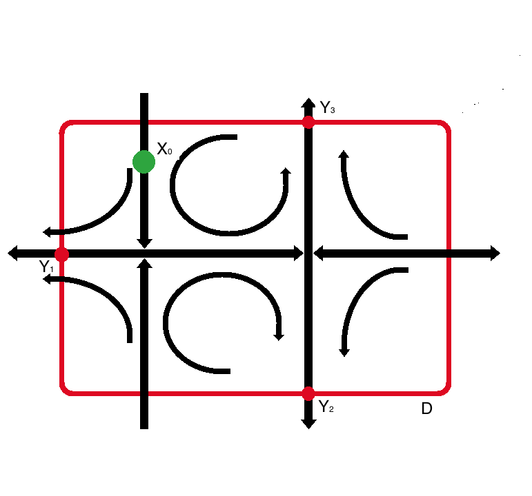
Refer to caption
Figure 1.4: Heteroclinic network example
Planar heteroclinic network with two nodes

Let us give a concrete example. Consider the system in which bb has two critical points {ζ1,ζ2}\{\zeta_{1},\zeta_{2}\} and phase space of the flow SS is as depicted in Figure 1.4, with DD being a rectangle around the two critical points. Let Xϵ​(0)=x0X_{\epsilon}(0)=x_{0} be on the locally stable manifold 𝒲1s\mathcal{W}^{s}_{1} of ζ1\zeta_{1}. Consider {qk+,qk−}=𝒲ku∩Bδ​(ζk)\{q_{k}^{+},q_{k}^{-}\}=\mathcal{W}_{k}^{u}\cap B_{\delta}(\zeta_{k}), where Bδ​(ζk)B_{\delta}(\zeta_{k}) is a ball of sufficiently small radius around ζk\zeta_{k} and 𝒲ku\mathcal{W}_{k}^{u} the locally unstable manifold of ζk\zeta_{k}. There is an orbit connecting ζ1\zeta_{1} with ζ2\zeta_{2}:

limt→∞St​q1−=ζ2.\lim_{t\ \to\infty}S^{t}q_{1}^{-}=\zeta_{2}.

Recall from Section 1.1 that as ϵ→\epsilon\to the exit distribution concentrates near the minimizers of V⁡(x,⋅)V(x,\cdot) over the boundary of ∂D\partial D. For a heteroclinic network this means that the exit concentrates at all points in the boundary that can be reached from xx along a sequence of heteroclinic connections. In this case, these points are

y1=limt→∞St​q1+,y2=limt→∞St​q2+,\displaystyle y_{1}=\lim_{t\ \to\infty}S^{t}q_{1}^{+},\quad y_{2}=\lim_{t\ \to\infty}S^{t}q_{2}^{+},

and y3=limt→∞St​q2−y_{3}=\lim_{t\to\infty}S^{t}q_{2}^{-}. Then, the exit measure will weakly converge, as ϵ→0\epsilon\to 0, to

p1​δy1+p2​δy2+p3​δy3,p_{1}\delta_{y_{1}}+p_{2}\delta_{y_{2}}+p_{3}\delta_{y_{3}}, (1.24)

where p1,p2p_{1},p_{2} and p3p_{3} are positive numbers that sum up to 11. In the spirit of Theorem 9 a direct application of our results imply a scaling limit to this convergence.

Lemma 16

Consider the system just described. There is a family of random variables (θϵ)ϵ>0(\theta_{\epsilon})_{\epsilon>0}, a family of random vectors (ϕϵ)ϵ>0(\phi_{\epsilon})_{\epsilon>0} and the random variable α0\alpha_{0} such that 𝐏{θϵ∈{1,2,3}}=𝐏{α0∈(0,1]}=1\mathbf{P}\{\theta_{\epsilon}\in\{1,2,3\}\}=\mathbf{P}\{\alpha_{0}\in(0,1]\}=1, and

Xϵ​(τϵD)=yθϵ+ϵα0​ϕϵ,X_{\epsilon}(\tau_{\epsilon}^{D})=y_{\theta_{\epsilon}}+\epsilon^{\alpha_{0}}\phi_{\epsilon},

for every ϵ>0\epsilon>0. The random vector (θϵ,ϕϵ)(\theta_{\epsilon},\phi_{\epsilon}) converges in distribution to (θ0,ϕ0)(\theta_{0},\phi_{0}).

The random vector (θ0,ϕ0)(\theta_{0},\phi_{0}) in principle can be obtained explicitly. It is clear from (1.24) that pi=𝐏{θ0=i}p_{i}=\mathbf{P}\{\theta_{0}=i\}, i=1,2,3i=1,2,3.

Let {λ+,−λ−}\{\lambda_{+},-\lambda_{-}\} be the set of eigenvalues of ∇b​(ζ1)\nabla b(\zeta_{1}) and {μ+,−μ−}\{\mu_{+},-\mu_{-}\} the set of eigenvalues of ∇b​(ζ2)\nabla b(\zeta_{2}) (see Figure 1.4). Using the three observations made at the beginning of Section 1.2.2 several cases can be considered (see [6] for further explanation):

  • •

    If μ+<μ−\mu_{+}<\mu_{-} , and λ+<λ−\lambda_{+}<\lambda_{-} then the system is symmetric with p1=1/2p_{1}=1/2, p2=p3=1/4p_{2}=p_{3}=1/4, and α0=1\alpha_{0}=1. Here symmetric means that the random vector ϕ0\phi_{0} has no bias along the direction of 𝒲1s\mathcal{W}_{1}^{s} if θ0=1\theta_{0}=1 or along the direction 𝒲1u\mathcal{W}^{u}_{1} if θ0∈{2,3}\theta_{0}\in\{2,3\}. Asymmetric means that there is a bias in any of the aforementioned cases.

  • •

    If μ+​λ+<μ−​λ−\mu_{+}\lambda_{+}<\mu_{-}\lambda_{-}, and λ+≥λ−\lambda_{+}\geq\lambda_{-}, the system is symmetric if θ0∈{2,3}\theta_{0}\in\{2,3\}, strongly asymmetric if λ+<λ−\lambda_{+}<\lambda_{-} and θ0=1\theta_{0}=1, and asymmetric if λ+=λ−\lambda_{+}=\lambda_{-} and θ0=1\theta_{0}=1. Moreover, p1=1/2p_{1}=1/2, p2=0,p3=1/2p_{2}=0,p_{3}=1/2, when λ−<λ+\lambda_{-}<\lambda_{+}, and p1=1/2,p2=0,p3=1/2p_{1}=1/2,p_{2}=0,p_{3}=1/2, when λ−=λ+\lambda_{-}=\lambda_{+}. The random variable α0\alpha_{0} is given by

    α0=λ−λ+​δ{1}​(θ0)+δ{2,3}​(θ0).\alpha_{0}=\frac{\lambda_{-}}{\lambda_{+}}\delta_{\{1\}}(\theta_{0})+\delta_{\{2,3\}}(\theta_{0}).
  • •

    If μ+​λ+>μ−​λ−\mu_{+}\lambda_{+}>\mu_{-}\lambda_{-}, and λ+>λ−\lambda_{+}>\lambda_{-}, the system is strongly asymmetric and p1=1/2p_{1}=1/2, p2=0,p3=1/2p_{2}=0,p_{3}=1/2, and

    α0=λ−λ+​δ{1}​(θ0)+μ−​λ−/(μ+​λ+)​δ{2,3}​(θ0).\alpha_{0}=\frac{\lambda_{-}}{\lambda_{+}}\delta_{\{1\}}(\theta_{0})+\mu_{-}\lambda_{-}/(\mu_{+}\lambda_{+})\delta_{\{2,3\}}(\theta_{0}).
  • •

    If μ+=μ−\mu_{+}=\mu_{-} and λ+=λ−\lambda_{+}=\lambda_{-}, the system is asymmetric and p1=1/2p_{1}=1/2, p2∈(0,p3),p3<1/2p_{2}\in(0,p_{3}),p_{3}<1/2, and α0=1\alpha_{0}=1.

  • •

    If μ+>μ−\mu_{+}>\mu_{-}, and λ+=λ−\lambda_{+}=\lambda_{-}, the system is asymmetric if θ0=1\theta_{0}=1 and strongly asymmetric otherwise. Moreover, p1=1/2p_{1}=1/2, p2∈(0,p3),p3<1/2p_{2}\in(0,p_{3}),p_{3}<1/2, and

    α0=δ{1}​(θ0)+(μ−/μ+)​δ{2,3}​(θ0).\alpha_{0}=\delta_{\{1\}}(\theta_{0})+(\mu_{-}/\mu_{+})\delta_{\{2,3\}}(\theta_{0}).
  • •

    If μ+=μ−\mu_{+}=\mu_{-}, and λ+>λ−\lambda_{+}>\lambda_{-}, the system is strongly asymmetric if θ0=1\theta_{0}=1, and asymmetric otherwise. Moreover, p1=1/2p_{1}=1/2, p2=0,p3=1/2p_{2}=0,p_{3}=1/2, and α0=λ−/λ+\alpha_{0}=\lambda_{-}/\lambda_{+}.

A formalization of this argument based on a weak convergence result is done in [4]. In such, the limiting behavior of the rescaled process

Zϵ​(t)=Xϵ​(t​log⁡(ϵ−1))Z_{\epsilon}(t)=X_{\epsilon}(t\log(\epsilon^{-1}))

is obtained. Notice how this rescaled process instantaneously jumps along saddles. Hence if a weak convergence result has to be established, we need to introduce a new topology. Indeed, the standard Skorokhod topology does not allow to capture the curves along which the jumps are made. We state the weak convergence result in the next section.

Weak convergence result

In order to present the weak convergence result for the rescaled version of XϵX_{\epsilon}, we need to introduce a new topology.

Consider all paths γ:[0,1]→[0,∞)×ℝ2\gamma:[0,1]\to[0,\infty)\times\mathbb{R}^{2} such that the first coordinate γ0\gamma^{0} is nondecreasing. Equip the space of paths with the equivalence relation ∼\sim, where γ1∼γ2\gamma_{1}\sim\gamma_{2} if and only if there is a path γ∗\gamma^{*} and non-decreasing surjective functions λ1,λ2:[0,1]→[0,1]\lambda_{1},\lambda_{2}:[0,1]\to[0,1] such that γi=γ∗∘λi\gamma_{i}=\gamma^{*}\circ\lambda_{i}. The set of curves 𝐗\mathbf{X} is the quotient of the space of paths with the equivalence relation ∼\sim. Actually the set 𝐗\mathbf{X} can be regarded as a Polish space:

Lemma 17 ( [4])

𝐗\mathbf{X} can be made into a metric Polish space with distance function

ρ⁡(Γ1,Γ2)=infγ1∈Γ1,γ2∈Γ2sups∈[0,1]|γ1​(s)−γ2​(s)|.\rho(\Gamma_{1},\Gamma_{2})=\inf_{\gamma_{1}\in\Gamma_{1},\gamma_{2}\in\Gamma_{2}}\sup_{s\in[0,1]}|\gamma_{1}(s)-\gamma_{2}(s)|.

Refer to [4] for more information about this sapce.

In order to state the result, we give a non-technical introduction to the notion of entrance-exit maps introduced in [4]. Let 𝒫\mathcal{P} be the set of probability measures in ℝ2\mathbb{R}^{2}, define out=(0,∞)×[0,1]×ℝ2×(0,1]×𝒫\rm{out}=(0,\infty)\times[0,1]\times\mathbb{R}^{2}\times(0,1]\times\mathcal{P} and

Outk={((t−,p−,x−,β−,F−),(t+,p+,x+,β+,F+))∈out2:\displaystyle\rm{Out}_{k}=\{\left((t_{-},p_{-},x_{-},\beta_{-},F_{-}),(t_{+},p_{+},x_{+},\beta_{+},F_{+})\right)\in\rm{out}^{2}:
t−=t+,x±=qk±,p−+p+=1,β−=β+}.\displaystyle t_{-}=t_{+},x_{\pm}=q_{k}^{\pm},p_{-}+p_{+}=1,\beta_{-}=\beta_{+}\}.

Then we have the following definitions.

Definition 18

For each kk, an entrance-exit map is a map

Ψk:{qk+,qk−}×(0,1]×𝒫→Outk,\Psi_{k}:\{q_{k}^{+},q_{k}^{-}\}\times(0,1]\times\mathcal{P}\to\rm{Out}_{k},

where the domain of Ψk\Psi_{k} satisfies some regularity assumptions(see [4, page 10] ) . We denote Ψk=(Ψk+,Ψk−)\Psi_{k}=(\Psi_{k}^{+},\Psi_{k}^{-}).

Definition 19

Suppose x0∈𝒲ksx_{0}\in\mathcal{W}^{s}_{k}, for some 1≤k≤N1\leq k\leq N. The sequence 𝐳=(θ0,zi1,…,θr−1,zir,θr)\mathbf{z}=(\theta_{0},z_{i_{1}},...,\theta_{r-1},z_{i_{r}},\theta_{r}) is admissible for x0x_{0} (refered as x0x_{0}-admissible) if

  1. 1.

    θ0\theta_{0} is the orbit of x0x_{0} with St​x0→zi1S^{t}x_{0}\to z_{i_{1}}, as t→∞t\to\infty;

  2. 2.

    for each j∈{1,..,r}j\in\{1,..,r\}, θj\theta_{j} is either the orbit of qij+q_{i_{j}}^{+} or the orbit qij−q_{i_{j}}^{-};

  3. 3.

    for each j∈{1,..,r}j\in\{1,..,r\}, ij+1i_{j+1} is either nij+n_{i_{j}}^{+} or nij−n_{i_{j}}^{-} according to whether t​h​e​t​ajtheta_{j} is the orbit of qij+q_{i_{j}}^{+} or qij−q_{i_{j}}^{-}.

With each admissible sequence 𝐳\mathbf{z} we associate the sequence

η⁡(𝐳)=((x0′,α0,μ0),(t1,p1,x1,α1,μ1),…,(tr,pr,xr,αr,μr)),\eta(\mathbf{z})=((x_{0}^{\prime},\alpha_{0},\mu_{0}),(t_{1},p_{1},x_{1},\alpha_{1},\mu_{1}),...,(t_{r},p_{r},x_{r},\alpha_{r},\mu_{r})),

where x0′=St′​(x0)​x0,α0=1x_{0}^{\prime}=S^{t^{\prime}(x_{0})}x_{0},\alpha_{0}=1,

t′​(x0)=inf{t>0:St​x0∈Bδ​(ζi1)},t^{\prime}(x_{0})=\inf\{t>0:S^{t}x_{0}\in B_{\delta}(\zeta_{i_{1}})\},

and the rest of the entries are given by

(tj,pj,xj,αj,μj)={Ψij+(xj−1,αj−1,μj−1),ij=nij+Ψij−(xj−1,αj−1,μj−1),ij=nij−.(t_{j},p_{j},x_{j},\alpha_{j},\mu_{j})=\left\{\begin{tabular}[]{ l r }$\Psi_{i_{j}}^{+}(x_{j-1},\alpha_{j-1},\mu_{j-1})$,&$i_{j}=n_{i_{j}}^{+}$\\ $\Psi_{i_{j}}^{-}(x_{j-1},\alpha_{j-1},\mu_{j-1})$,&$i_{j}=n_{i_{j}}^{-}$\\ \end{tabular}\right..

To each admissible sequence 𝐳\mathbf{z} we can associate a piecewise constant curve Γ⁡(𝐳)\Gamma(\mathbf{z}) by identifying it with the path of curves such that spend time tjt_{j} at the point xjx_{j} and jump to the next point along the path θj\theta_{j}. Also we can associate probabilities through the relationship

π⁡(𝐳)=p1​…​pr.\pi(\mathbf{z})=p_{1}...p_{r}.

Note how the set of all admissible sequences for x0x_{0} has the structure of a binary tree partially ordered by inclusion. We say that a set of admissible sequences LL of x0x_{0} is free if no two sequences of LL are comparable with respect to this partial order. Additionally, if any sequence not in LL is comparable to one sequence from LL then LL is called complete. It is clear that for any free set π⁡(L):=∑𝐳∈Lπ⁡(𝐳)≤1\pi(L):=\sum_{\mathbf{z}\in L}\pi(\mathbf{z})\leq 1, while for a complete set π⁡(L)=1\pi(L)=1.

The main theorem is:

Theorem 20

Suppose that Xϵ​(0)=x0X_{\epsilon}(0)=x_{0} is in the heteroclinic invariant. For each ϵ>0\epsilon>0, define the process Zϵ​(t)=Xϵ​(t​|log⁡(ϵ)|)Z_{\epsilon}(t)=X_{\epsilon}(t|\log(\epsilon)|). Then, for any conservative set LL of x0x_{0}-admissible sequences, there is a family of stopping times (Tϵ)ϵ>0(T_{\epsilon})_{\epsilon>0} such that the distribution of the graph ΓZϵ​(t),t<Tϵ\Gamma_{Z_{\epsilon}(t),t<T_{\epsilon}} converges weakly in (𝕏,ρ)(\mathbb{X},\rho) to the measure Mx0,LM_{x_{0},L} concentrated on the set

{Γ⁡(𝐳):𝐳∈L}\{\Gamma(\mathbf{z}):\mathbf{z}\in L\}

and satisfying MXϵ​(0),L​{Γ⁡(𝐳)}=π⁡(𝐳)M_{X_{\epsilon}(0),L}\{\Gamma(\mathbf{z})\}=\pi(\mathbf{z}).

Contributions made in the case SS admits a heteroclinic network

In this section we outline our contribution for the case in which SS admits an heteroclinic network.

The iteration procedure described in Section 1.4.2 was first proposed in [4]. It is the central idea in proving the main results in [4]. This iteration is carried out in [4] by using an equivalent version of Theorem 9. This version was proved under the hypothesis that the non-linear system can be locally conjugated to a linear system by a C2C^{2} transformation. That is, in [4] Theorem 20 is proved under the following hypothesis:

Condition 21

At each critical point ζ∈𝒵\zeta\in\mathcal{Z} there are non-resonant conditions.

As discussed in Section 1.2 this is in general not the case, and examples of saddle point that do not satisfy this condition are known [48]. In this work, we completely remove condition 21 in the 22-dimensional situation.

On the other hand, observe that the iteration procedure is Section 1.4.2 is based on the computation of a random map. This map is such that, for a domain VV, to any given initial distribution of the diffusion XϵX_{\epsilon}, it gives the exit distribution of XϵX_{\epsilon} from VV. We call this map a random Poincaré map. For V⊂ℝ2V\subset\mathbb{R}^{2}, let ΠV\Pi_{V} be the set of probability measures with support on VV. Then, the random Poincaré map for DD, ΥD:ΠD→Π∂D\Upsilon_{D}:\Pi_{D}\to\Pi_{\partial D} is the (deterministic) map such that ΥD𝐐=𝐏𝐐{Xϵ(τϵD}\Upsilon_{D}\mathbf{Q}=\mathbf{P}_{\mathbf{Q}}\{X_{\epsilon}(\tau_{\epsilon}^{D}\}, where 𝐏𝐐\mathbf{P}_{\mathbf{Q}} is the original probability measure conditioned on Xϵ​(0)X_{\epsilon}(0) being distributed as 𝐐\mathbf{Q}. The iteration in Section 1.4.2 illustrates the use of this map. Notice that this methodology applies regardless the type of equilibria that the system exhibits. We base our proof of Theorems 9 and 13 on a similar idea. Hence, it is worth to study small noise perturbations with this direction in mind.

As an example of a Poincaré map, consider our example in Section 1.4.2. The exit distribution is the composition of the Poincaré maps ΥD5∘…∘ΥD1​δx0\Upsilon_{D_{5}}\circ...\circ\Upsilon_{D_{1}}\delta_{x_{0}}, where DiD_{i} are ilustrated in Figures 1.5 and , and we are conditioning on exit along y3y_{3}.

Refer to caption
Figure 1.5: Illustration of the domains D1D_{1}, D2D_{2}, and D3D_{3} used to compute the Poincaré maps in the case of a heteroclinic network with 2 nodes conditioned on exit along y3y_{3}: escape from the first saddle.
Refer to caption
Figure 1.6: Illustration of the domains D3D_{3} and D4D_{4} used to compute the Poincaré maps in the case of a heteroclinic network with 2 nodes condition on exit along y3y_{3}: escape from the second saddle.

1.5 General Setting

The objective of this section is to establish the general setting and notation, although each chapter has the necessary modifications and additions to the following.

Let (Ω,ℱ,𝐏)(\Omega,\mathcal{F},\mathbf{P}) be a complete probability space (every subset of every measurable null set is measurable) and WW be a dd-dimensional standard Brownian Motion on it. Let (ℱtW)t>0(\mathcal{F}^{W}_{t})_{t>0} be the filtration generated by WW which satisfies the usual hypothesis [54, Section I.5] . We assume that (Ω,ℱ,𝐏)(\Omega,\mathcal{F},\mathbf{P}) is rich enough to accommodate a family of random vectors (ξϵ)ϵ≥0(\xi_{\epsilon})_{\epsilon\geq 0} in ℝd\mathbb{R}^{d} such that the sigma algebra generated by ξϵ\xi_{\epsilon} is independent of ℱ∞W\mathcal{F}_{\infty}^{W} for each ϵ>0\epsilon>0. For each ϵ>0\epsilon>0, we consider the left continuous filtration

𝒢tϵ=σ⁡(ξϵ)∨ℱtW,\mathcal{G}^{\epsilon}_{t}=\sigma(\xi_{\epsilon})\vee\mathcal{F}_{t}^{W},

as well as the collection of null sets

N0={Z⊂Ω:∃G∈𝒢∞ϵ​ with ​Z⊂G​ and ​𝐏​{G}=0}.N_{0}=\{Z\subset\Omega:\exists G\in\mathcal{G}^{\epsilon}_{\infty}\text{ with }Z\subset G\text{ and }\mathbf{P}\{G\}=0\}.

Let us create the augmented filtration ℱtϵ=σ⁡(𝒢tϵ∪N0)\mathcal{F}_{t}^{\epsilon}=\sigma(\mathcal{G}_{t}^{\epsilon}\cup N_{0}) for t∈[0,∞)t\in[0,\infty), and ℱ∞ϵ=σ(∪t≥0ℱtϵ)\mathcal{F}^{\epsilon}_{\infty}=\sigma(\cup_{t\geq 0}\mathcal{F}_{t}^{\epsilon}). It can be shown that WW is a brownian motion with respect to (ℱtϵ)t≥0(\mathcal{F}^{\epsilon}_{t})_{t\geq 0}, the path of WW is independent of ξϵ\xi_{\epsilon} and (ℱtϵ)t≥0(\mathcal{F}^{\epsilon}_{t})_{t\geq 0} satisfies the usual hypothesis, for every ϵ>0\epsilon>0.

Throughout the text, we suppose that the family of random variables (ξϵ)ϵ≥0(\xi_{\epsilon})_{\epsilon\geq 0} satisfies ξϵ→ξ0\xi_{\epsilon}\to\xi_{0} in distribution, and that ξϵ\xi_{\epsilon} has a finite second moment for each ϵ>0\epsilon>0.

Consider a C∞C^{\infty}-smooth vector field bb on ℝd\mathbb{R}^{d} and a C2C^{2}-smooth matrix valued function σ:ℝd→ℝd×d\sigma:\mathbb{R}^{d}\to\mathbb{R}^{d\times d}. Consider the Itô stochastic differential equation

d​Xϵ=b⁡(Xϵ)​d​t+ϵ​σ​(Xϵ)​d​WdX_{\epsilon}=b(X_{\epsilon})dt+\epsilon\sigma(X_{\epsilon})dW (1.25)

equipped with initial condition

Xϵ​(0)=x0+ϵα​ξϵ,X_{\epsilon}(0)=x_{0}+\epsilon^{\alpha}\xi_{\epsilon}, (1.26)

where α∈(0,1]\alpha\in(0,1]. Hypothesis regarding the point x0∈ℝdx_{0}\in\mathbb{R}^{d} will be given in each chapter. We assume that both bb and σ\sigma are uniformly Lipschitz and bounded, i.e., there is a constant L>0L>0 such that

|σ⁡(x)−σ⁡(y)|∨|b⁡(x)−b⁡(y)|\displaystyle|\sigma(x)-\sigma(y)|\vee|b(x)-b(y)| ≤L​|x−y|,x,y∈ℝ2,\displaystyle\leq L|x-y|,\quad x,y\in\mathbb{R}^{2},
|σ⁡(x)|∨|b⁡(x)|\displaystyle|\sigma(x)|\vee|b(x)| ≤L,x∈ℝ2,\displaystyle\leq L,\quad x\in\mathbb{R}^{2},

where |⋅||\cdot| denotes the Euclidean norm for vectors and Hilbert–Schmidt norm for matrices. Further assume that the matrix function a=σ​σ∗a=\sigma\sigma^{*} is uniformly positive definite. These conditions can be weakened, but we prefer this setting to avoid multiple localization procedures throughout the text. These assumptions imply [41, Theorems 5.2.5 and 5.2.9] that equation (1.25) has a strong solution with strong uniqueness on the filtered probability space (Ω,ℱ,𝐏,(ℱtϵ)t≥0)(\Omega,\mathcal{F},\mathbf{P},(\mathcal{F}^{\epsilon}_{t})_{t\geq 0}) with initial condition (1.26) for each ϵ>0\epsilon>0. Let us recall the definition of strong uniqueness and strong solution for completeness.

Definition 22

A strong solution of the stochastic differential equation (1.25) with initial condition (1.26) on the filtered probability space (Ω,ℱ,𝐏,(ℱtϵ)t≥0)(\Omega,\mathcal{F},\mathbf{P},(\mathcal{F}^{\epsilon}_{t})_{t\geq 0}) is a process Xϵ={Xϵ(t);0≤t<∞}X_{\epsilon}=\{X_{\epsilon}(t);0\leq t<\infty\} with continuous sample paths and with the following properties:

  1. 1.

    XϵX_{\epsilon} is adapted to the filtration (ℱtϵ)t≥0(\mathcal{F}^{\epsilon}_{t})_{t\geq 0},

  2. 2.

    𝐏{Xϵ(0)=x0+ϵαξϵ}=1\mathbf{P}\{X_{\epsilon}(0)=x_{0}+\epsilon^{\alpha}\xi_{\epsilon}\}=1,

  3. 3.

    𝐏{∫0t(|bi(Xϵ(s))|+σi,j(Xϵ(s))2)ds<∞}=1\mathbf{P}\{\int_{0}^{t}(|b_{i}(X_{\epsilon}(s))|+\sigma_{i,j}(X_{\epsilon}(s))^{2})ds<\infty\}=1 for every 1≤i,j≤d1\leq i,j\leq d and t≥0t\geq 0,

  4. 4.

    the integral version of (1.25)

    Xϵ​(t)=Xϵ​(0)+∫0tb⁡(Xϵ​(s))​𝑑s+ϵ​∫0tσ⁡(Xϵ​(s))​𝑑W​(s);0≤t<∞,X_{\epsilon}(t)=X_{\epsilon}(0)+\int_{0}^{t}b(X_{\epsilon}(s))ds+\epsilon\int_{0}^{t}\sigma(X_{\epsilon}(s))dW(s);0\leq t<\infty,

    holds with probability 11.

Given two strong solutions XϵX_{\epsilon} and X~ϵ\widetilde{X}_{\epsilon} of (1.25) with initial condition (1.26) relative to the same brownian motion WW. Then, we say that strong uniqueness holds whenever 𝐏{Xϵ(t)=X~ϵ(t);0≤t<∞}=1\mathbf{P}\{X_{\epsilon}(t)=\widetilde{X}_{\epsilon}(t);0\leq t<\infty\}=1.

For a general background on stochastic differential equations see, for example, [41, Chapter 5].

The flow generated by bb is denoted by S=(St​x)(t,x)∈ℝ×ℝdS=(S^{t}x)_{(t,x)\in\mathbb{R}\times\mathbb{R}^{d}}. That is, St​xS^{t}x satisfies

dd​t​St​x=b⁡(St​x),S0​x=x.\frac{d}{dt}S^{t}x=b(S^{t}x),\quad S^{0}x=x.

The linearization of SS along the orbit of xx is denoted by Φx​(t)\Phi_{x}(t):

dd​t​Φx​(t)=A⁡(t)​Φx​(t)​, ​Φx​(0)=I,\frac{d}{dt}\Phi_{x}(t)=A(t)\Phi_{x}(t)\text{, \ }\Phi_{x}(0)=I, (1.27)

where A⁡(t)=∇b​(St​x)A(t)=\nabla b(S^{t}x) and II is the identity matrix. Here ∇\nabla is the derivative operator, that is, for a differentiable vector field h:ℝd→ℝdh:\mathbb{R}^{d}\to\mathbb{R}^{d}, ∇h\nabla h is the ℝd×d\mathbb{R}^{d\times d} matrix derivative of hh.

Throughout the text DD is a domain (open, connected and bounded) in ℝd\mathbb{R}^{d} with piecewise C2C^{2} boundary.

The exit problem for the diffusion process XϵX_{\epsilon} in DD is studied. We are interested in the joint asymptotic properties (as ϵ→0\epsilon\to 0) of (Xϵ​(τϵD),τϵD)(X_{\epsilon}(\tau_{\epsilon}^{D}),\tau_{\epsilon}^{D}), where τϵD\tau_{\epsilon}^{D} is the stopping time defined by

τϵD=τϵD​(x0)=inf{t>0:Xϵ​(t)∈∂D}.\tau_{\epsilon}^{D}=\tau_{\epsilon}^{D}(x_{0})=\inf\{t>0:X_{\epsilon}(t)\in\partial D\}.

.

Specific hypotheses on the vector field will be given in each chapter. On the other hand, the abstract formulation will not be given in each chapter, instead we assume this technical formulation to hold throughout the text.

1.5.1 Organization of the Text

The organization of the rest of the text closely mimics the presentation given in this chapter.

In Chapter 2 the planar (i.e. d=2d=2) exit problem is studied under the assumption that SS has a unique saddle at the origin. That is, 0∈ℝ20\in\mathbb{R}^{2} is the only critical point b⁡(0)=0b(0)=0 and the eigenvalues λ+\lambda_{+}, −λ−-\lambda_{-} of the of the matrix ∇b​(0)\nabla b(0) are such that λ±>0\lambda_{\pm}>0. The exit problem is studied conditioned that the process XϵX_{\epsilon} starts on the stable manifold 𝒲s\mathcal{W}^{s} of 00.

In Chapter 3 the Levinson case in arbitrary dimensions is considered. We also proved Lemma 12 stated in this chapter, and use it intesively in the proof of the Levinson case. In this section, we also study the 11-dimensional example discussed in Section 1.4.1 of this chapter.

In Chapter 4 we present a short survey on how the techniques in this text can be extended. Several open problems are also discussed.

Chapter 2 Saddle Point

In this chapter we study the stochastic process XϵX_{\epsilon} when the underlying deterministic system SS has a unique saddle point.

In Section 2.1 we introduce the setting, which relies on the setting presented in Section  1.5 of Chapter 1. In Section 2.2 we state the main theorem and split the proof into several parts. In Section 2.3 we introduce a simplifying change of coordinates in a small neigborhood of the saddle point. The analysis of the transformed process in Section 2.4 is based upon two results. Their proofs are given in Sections 2.5 and 2.6.

2.1 Setting

For this chapter we consider the general formulation made in Section 1.5 of Chapter 1, except that we restrict ourselves to the 2−2-dimensional situation. The process XϵX_{\epsilon} is the strong solution of (1.25), under the assumptions made on the C∞C^{\infty}-smooth vector field bb, the C2C^{2}-smooth matrix valued function σ:ℝ2→ℝ2×2\sigma:\mathbb{R}^{2}\to\mathbb{R}^{2\times 2} and the standard 22-dimensional Wiener process WW in Section 1.5 of Chapter 1.

We will study the exit problem from the domain D⊂ℝ2D\subset\mathbb{R}^{2} with piecewise C2C^{2} boundary. Assume that the origin 00 belongs to DD and it is a unique fixed point for SS in D¯\bar{D}, or, equivalently, a unique critical point for bb in D¯\bar{D}. Therefore,

b⁡(x)=A​x+Q⁡(x),b(x)=Ax+Q(x),

where A=∇b​(0)A=\nabla b(0) and QQ is the non-linear part of the vector field satisfying |Q⁡(x)|=O⁡(|x|2)|Q(x)|=O(|x|^{2}), x→0x\to 0.

Suppose that 00 is a hyperbolic critical point, i.e. the matrix AA has two eigenvalues λ+\lambda_{+} and −λ−-\lambda_{-} satisfying −λ−<0<λ+-\lambda_{-}<0<\lambda_{+}. Without loss of generality, we suppose that the canonical vectors are the eigenvectors for the matrix, so that A=diag(λ+,−λ−)A=\mathop{\mathrm{diag}}(\lambda_{+},-\lambda_{-}).

For an interval J⊂ℝJ\subset\mathbb{R}, let SJ​xS^{J}x denote the set

SJ​x={St​x:t∈J}.S^{J}x=\{S^{t}x:t\in J\}.

According to the Hadamard–Perron Theorem (see e.g. [53, Section 2.7]), the curves 𝒲s\mathcal{W}^{s} and 𝒲u\mathcal{W}^{u} defined via

𝒲u\displaystyle\mathcal{W}^{u} ={x∈D¯:limt→−∞Stx=0, and for some s≥0,S(−∞,s)x⊂D and S(s,∞)x∩D¯=∅},\displaystyle=\{x\in\bar{D}:\lim_{t\to-\infty}S^{t}x=0\text{, and for some }s\geq 0,S^{(-\infty,s)}x\subset D\text{ and }S^{(s,\infty)}x\cap\bar{D}=\emptyset\},

and,

𝒲s={x∈D¯:limt→∞Stx=0, and for some s≤0,S(−∞,s)x∩D¯=∅ and S(s,∞)x⊂D}.\mathcal{W}^{s}=\{x\in\bar{D}:\lim_{t\to\infty}S^{t}x=0\text{, and for some }s\leq 0,S^{(-\infty,s)}x\cap\bar{D}=\emptyset\text{ and }S^{(s,\infty)}x\subset D\}.

are smooth, invariant under SS and tangent to e2e_{2} and, respectively, to e1e_{1} at 00. The curve 𝒲s\mathcal{W}^{s} is called the stable manifold of 00, and 𝒲u\mathcal{W}^{u} is called the unstable manifold of 00.

We assume that 𝒲u\mathcal{W}^{u} intersects ∂D\partial D transversally at points q+q_{+} and q−q_{-} such that the segment of 𝒲u\mathcal{W}^{u} connecting q−q_{-} and q+q_{+} lies entirely inside DD and contains 00.

We fix a point x0∈𝒲s∩Dx_{0}\in\mathcal{W}^{s}\cap D and equip (1.25) with the initial condition

Xϵ​(0)=x0+ϵα​ξϵ,ϵ>0,X_{\epsilon}(0)=x_{0}+\epsilon^{\alpha}\xi_{\epsilon},\quad\epsilon>0, (2.1)

where α∈(0,1]\alpha\in(0,1] is fixed, and (ξϵ)ϵ>0(\xi_{\epsilon})_{\epsilon>0} is a family of random vectors independent of WW, such that for some random vector ξ0\xi_{0}, ξϵ→ξ0\xi_{\epsilon}\rightarrow\xi_{0} as ϵ→0\epsilon\rightarrow 0 in distribution.

If α≠1\alpha\neq 1, then we impose a further technical condition

𝐏{ξ0∥b(x0)}=0,\mathbf{P}\{\xi_{0}\parallel b(x_{0})\}=0, (2.2)

where ∥\parallel denotes collinearity of two vectors.

2.2 Main Result.

The main result of the present chapter is the following:

Theorem 23

In the setting described above, there is a family of random vectors (ϕϵ)ϵ>0(\phi_{\epsilon})_{\epsilon>0}, a family of random variables (ψϵ)ϵ>0(\psi_{\epsilon})_{\epsilon>0}, and a number

β={1,α​λ−≥λ+α​λ−λ+,α​λ−<λ+\beta=\left\{\begin{array}[]{cc}1,&\alpha\lambda_{-}\geq\lambda_{+}\\ \alpha\frac{\lambda_{-}}{\lambda_{+}},&\alpha\lambda_{-}<\lambda_{+}\\ \end{array}\right. (2.3)

such that

Xϵ​(τϵD)=qsgn(ψϵ)+ϵβ​ϕϵ.X_{\epsilon}(\tau_{\epsilon}^{D})=q_{\mathop{\mathrm{sgn}}(\psi_{\epsilon})}+\epsilon^{\beta}\phi_{\epsilon}.

The random vector

Θϵ=(ψϵ,ϕϵ,τϵD+αλ+​ln⁡ϵ)\Theta_{\epsilon}=\left(\psi_{\epsilon},\phi_{\epsilon},\tau_{\epsilon}^{D}+\frac{\alpha}{\lambda_{+}}\ln\epsilon\right)

converges in distribution as ϵ→0\epsilon\to 0.

The distribution of ψϵ\psi_{\epsilon},ϕϵ\phi_{\epsilon}, and the distributional limit of Θϵ\Theta_{\epsilon} will be described precisely.

The proof of Theorem 23 has essentially three parts involving the analysis of diffusion (i) along 𝒲s\mathcal{W}^{s}; (ii) in a small neighborhood of the origin; (iii) along 𝒲u\mathcal{W}^{u}.

In order to study the first part, we need to introduce Φx​(t)\Phi_{x}(t) as the linearization of SS along the orbit of x∈ℝ2x\in\mathbb{R}^{2}, i.e. we define Φx​(t)\Phi_{x}(t) to be the solution to the matrix ODE

dd​t​Φx​(t)=A⁡(t)​Φx​(t)​, ​Φx​(0)=I,\frac{d}{dt}\Phi_{x}(t)=A(t)\Phi_{x}(t)\text{, \ }\Phi_{x}(0)=I,

where A⁡(t)=∇b​(St​x)A(t)=\nabla b(S^{t}x). We have the following theorem:

Theorem 24

Let x∈ℝ2x\in\mathbb{R}^{2} and (ξϵ)ϵ>0\left(\xi_{\epsilon}\right)_{\epsilon>0} be a family of random vectors independent of WW and convergent in distribution, as ϵ→0\epsilon\to 0, to ξ0\xi_{0}. Suppose α∈(0,1]\alpha\in(0,1] and let XϵX_{\epsilon} be the solution of the SDE (1.25) with initial condition Xϵ​(0)=x+ϵα​ξϵX_{\epsilon}(0)=x+\epsilon^{\alpha}\xi_{\epsilon}. Then, for every T>0T>0, the following representation holds true:

Xϵ​(T)=ST​x+ϵα​ξ¯ϵ,ϵ>0,X_{\epsilon}(T)=S^{T}x+\epsilon^{\alpha}\bar{\xi}_{\epsilon},\quad\epsilon>0,

where

ξ¯ϵ​⟶L​a​w​ξ¯0,ϵ→0,\bar{\xi}_{\epsilon}\overset{\mathop{Law}}{\longrightarrow}\bar{\xi}_{0},\quad\epsilon\to 0,

with

ξ¯0=Φx(T)ξ0+𝟏{α=1}N,\bar{\xi}_{0}=\Phi_{x}(T)\xi_{0}+\mathbf{1}_{\{\alpha=1\}}N,

NN being a Gaussian vector:

N=Φx​(T)​∫0TΦx​(s)−1​σ​(Ss​x)​𝑑W​(s).N=\Phi_{x}(T)\int_{0}^{T}\Phi_{x}(s)^{-1}\sigma(S^{s}x)dW(s).

If α=1\alpha=1 or assumption (2.2) holds, then 𝐏{ξ¯0∥b(STx)}=0\mathbf{P}\{\bar{\xi}_{0}\parallel b({S^{T}x})\}=0.

The second part of the analysis is the core of the chapter. Theorem 25 below describes the behavior of the process in a small neighborhood UU of the origin. Notice that since x0∈𝒲sx_{0}\in\mathcal{W}^{s}, one can choose TT large enough to ensure that that ST​x0∈𝒲s∩US^{T}x_{0}\in\mathcal{W}^{s}\cap U. Therefore, the conditions of the following result are met if we use the terminal distribution of Theorem 24 (applied to the initial data given by (2.1)) as the initial distribution.

Theorem 25

There are two neighborhoods of the origin U⊂U′⊂DU\subset U^{\prime}\subset D, two positive numbers δ<δ′\delta<~\delta^{\prime}, and C2C^{2} diffeomorphism f:U′→(−δ′,δ′)2f:U^{\prime}\to(-\delta^{\prime},\delta^{\prime})^{2}, such that f⁡(U)=(−δ,δ)2f(U)=(-\delta,\delta)^{2} and the following property holds:

Suppose x∈𝒲s∩Ux\in\mathcal{W}^{s}\cap U, and (ξϵ)ϵ>0(\xi_{\epsilon})_{\epsilon>0} is a family of random variables independent of WW and convergent in distribution, as ϵ→0\epsilon\to 0, to ξ0\xi_{0}, where ξ0\xi_{0} satisfies (2.2) with respect to xx. Assume that α∈(0,1]\alpha\in(0,1] and that XϵX_{\epsilon} solves (1.25) with initial condition

Xϵ​(0)=x+ϵα​ξϵ,X_{\epsilon}(0)=x+\epsilon^{\alpha}\xi_{\epsilon}, (2.4)

where ξϵ\xi_{\epsilon} satisfies condition (2.2) with respect to xx.

There is also a family of random vectors (ϕϵ′)ϵ>0(\phi^{\prime}_{\epsilon})_{\epsilon>0}, and a family of random variables (ψϵ′)ϵ>0,(\psi^{\prime}_{\epsilon})_{\epsilon>0}, such that

Xϵ​(τϵU)=g⁡(sgn(ψϵ′)​δ​e1)+ϵβ​ϕϵ′,X_{\epsilon}(\tau_{\epsilon}^{U})=g(\mathop{\mathrm{sgn}}(\psi^{\prime}_{\epsilon})\delta e_{1})+\epsilon^{\beta}\phi^{\prime}_{\epsilon},

where g=f−1g=f^{-1}, β\beta is defined in (2.3), and the random vector

Θϵ′=(ψϵ′,ϕϵ′,τϵU+αλ+​ln⁡ϵ)\Theta^{\prime}_{\epsilon}=\left(\psi^{\prime}_{\epsilon},\phi^{\prime}_{\epsilon},\tau_{\epsilon}^{U}+\frac{\alpha}{\lambda_{+}}\ln\epsilon\right)

converges in distribution as ϵ→0\epsilon\to 0.

The notation for Θϵ′\Theta^{\prime}_{\epsilon} and its components is chosen to match the notation involved in the statement of Theorem 23. Random elements ψϵ′\psi^{\prime}_{\epsilon},ϕϵ′\phi^{\prime}_{\epsilon} and the distributional limit of Θϵ′\Theta^{\prime}_{\epsilon} will be described precisely, see (2.30). Obviously, the symmetry or asymmetry in the limiting distribution of ψϵ′\psi^{\prime}_{\epsilon} results in the symmetric or asymmetric choice of exit direction so that the exits in the positive and negative directions are equiprobable or not. On the other hand, the limiting distribution of ϕϵ′\phi^{\prime}_{\epsilon} determining the asymptotics of the exit point can also be symmetric or asymmetric which results in the corresponding features of the random choice of the exit direction at the next saddle point visited by the diffusion.

In Section 2.4 we prove Theorem 25 using the approach based on normal forms.

The last part of the analysis is devoted to the exit from DD along 𝒲u\mathcal{W}^{u}. We need the following statement which is a specific case of the main result of Chapter 3.

Theorem 26

In the setting of Theorem 24, assume additionally that (i) q=ST​x∈∂Dq=S^{T}x\in\partial D; (ii) there is no t∈[0,T)t\in[0,T) with St​x∈∂DS^{t}x\in\partial D; (iii) b⁡(q)b(q) is tranversal (i.e. not tangent) to ∂D\partial D at qq. Then

τϵD→𝐏T,ϵ→0,\tau_{\epsilon}^{D}\stackrel{{\scriptstyle\mathbf{P}}}{{\to}}T,\quad\epsilon\to 0, (2.5)

and

ϵ−α​(Xϵ​(τϵD)−q)→L​a​wπ​ξ¯0,ϵ→0,\epsilon^{-\alpha}(X_{\epsilon}(\tau_{\epsilon}^{D})-q)\stackrel{{\scriptstyle Law}}{{\to}}\pi\bar{\xi}_{0},\quad\epsilon\to 0, (2.6)

where π\pi denotes the projection along b⁡(q)b(q) onto the tangent line to ∂D\partial D at qq.

Now Theorem 23 follows from the consecutive application of Theorems 24 through 26 and with the help of the strong Markov property. In fact, in this chain of theorems, the conclusion of Theorem 24 ensures that the conditions of Theorem 25 hold, and the conclusion of the latter ensures that the conditions of Theorem 26 hold. Notice that the total time needed to exit DD equals the sum of times described in the three theorems. Notice also that at each step we can compute the limiting initial and terminal distributions explicitly. Theorems 24 and 26 contain the respective formulas in their formulations, and the explicit limiting distribution for Θϵ′\Theta^{\prime}_{\epsilon} of Theorem 25 is computed in (2.30).

2.3 Simplifying change of coordinates

2.3.1 Smooth Transformation and Normal Forms

In this section we give a brief review of the theory of Normal Forms. In particular, we focus on the neighborhood of a saddle point for the deterministic flow SS.

The idea is to find a local change of variables θ:ℝ2→ℝ2\theta:\mathbb{R}^{2}\to\mathbb{R}^{2} such that z⁡(t)=θ⁡(St​x)z(t)=\theta(S^{t}x) satisfies z˙=A​z\dot{z}=Az with the appropriate initial condition. First, note that zz satisfies the equation

dd​t​z​(t)\displaystyle\frac{d}{dt}z(t) =∇θ​(St​x)​b​(St​x)\displaystyle=\nabla\theta(S^{t}x)b(S^{t}x)
=∇θ(z(t))−1b(θ−1(z(t))),z(0)=θ(x).\displaystyle=\nabla\theta(z(t))^{-1}b(\theta^{-1}(z(t))),\quad z(0)=\theta(x).

Hence, the goal is to find a transformation θ:ℝ2→ℝ2\theta:\mathbb{R}^{2}\to\mathbb{R}^{2} that leaves ∇θ(z)−1b(θ−1(z))\nabla\theta(z)^{-1}b(\theta^{-1}(z)) as simple as possible (ideally equal to A​zAz).

We start with some notions. For a multi-index α=(α1,α2)∈ℤ+2\alpha=(\alpha_{1},\alpha_{2})\in\mathbb{Z}_{+}^{2} and a base {e1,e2}\{e_{1},e_{2}\} of ℝ2\mathbb{R}^{2}(as a vector space over ℝ\mathbb{R}) we denote the monomial xα​ei=x1α1​x2α2​eix^{\alpha}e_{i}=x_{1}^{\alpha_{1}}x_{2}^{\alpha_{2}}e_{i}.

Definition 27

For a non-negative integer rr, the space of linear combinations (over ℝ\mathbb{R}) of monomials xα​eix^{\alpha}e_{i} with |α|=α1+α2=r|\alpha|=\alpha_{1}+\alpha_{2}=r, is called the space of Homogenous Polynomials in 22 variables of degree rr. This space is denoted as ℋr\mathcal{H}_{r}. In other words, ℋr\mathcal{H}_{r} is,

ℋr=spanℝ{xαej:α∈ℤ+2,|α|=r and 1≤j≤2}.\mathcal{H}_{r}=\rm{span}_{\mathbb{R}}\left\{x^{\alpha}e_{j}:\alpha\in\mathbb{Z}_{+}^{2},|\alpha|=r\text{ and }1\leq j\leq 2\right\}.

It is easy to see that ℋr\mathcal{H}_{r} is isomorphic (as a vector space over the real numbers) to ℝ2​(r+1)\mathbb{R}^{2(r+1)}.

Using this notation, use Taylor’s classical theorem to decompose the function b:ℝ2→ℝ2b:\mathbb{R}^{2}\rightarrow\mathbb{R}^{2} as

b⁡(z)=A​z+b2​(z)+…+bR​(z),b(z)=Az+b_{2}(z)+...+b_{R}(z), (2.7)

with bi∈ℋib_{i}\in\mathcal{H}_{i} for 1≤i≤R1\leq i\leq R, and bR​(x)=O⁡(|x|R)b_{R}(x)=O(|x|^{R}) as |x|→0|x|\to 0.

Suppose that z=θk​(ζ)z=\theta_{k}(\zeta), where θk\theta_{k} is the near identity transformation

θk​(ζ)=ζ+hk​(ζ),hk∈ℋk,k≥2.\theta_{k}(\zeta)=\zeta+h_{k}(\zeta),\quad h_{k}\in\mathcal{H}_{k},\quad k\geq 2. (2.8)

Note that θk\theta_{k} is a topological diffeomorphism in a small open neighborhood of the origin Ωk\Omega_{k}. Throughout we restrict the analysis inside Ωk\Omega_{k}. A Taylor approximation shows that the inverse of θk\theta_{k} satisfies

θk−1​(ζ)\displaystyle\theta_{k}^{-1}(\zeta) =ζ−hk​(ζ)+O⁡(|ζ|2​k−1)\displaystyle=\zeta-h_{k}(\zeta)+O(|\zeta|^{2k-1})
=ζ−hk​(ζ)+O⁡(|ζ|k+1).\displaystyle=\zeta-h_{k}(\zeta)+O(|\zeta|^{k+1}). (2.9)

Further application of Taylor’s approximation together with the condition that k≥2k\geq 2, imply that for any ζ∈Ωk\zeta\in\Omega_{k},

∇θk(ζ)−1\displaystyle\nabla\theta_{k}(\zeta)^{-1} =I−∇hk​(ζ)+O⁡(|ζ|2​(k−1))\displaystyle=I-\nabla h_{k}(\zeta)+O(|\zeta|^{2(k-1)})
=I−∇hk​(ζ)+O⁡(|ζ|k).\displaystyle=I-\nabla h_{k}(\zeta)+O(|\zeta|^{k}).

Also, from (2.9), we obtain that for any i=1,…,R−1i=1,...,R-1,

bi​(θk−1​(ζ))=bi​(ζ)+O⁡(|ζ|k+1).b_{i}(\theta^{-1}_{k}(\zeta))=b_{i}(\zeta)+O(|\zeta|^{k+1}).

Using (2.7) and this bounds, we get that

(∇θk​(ζ))−1​b​(θk−1​(ζ))\displaystyle(\nabla\theta_{k}(\zeta))^{-1}b(\theta_{k}^{-1}(\zeta)) =\displaystyle= A​ζ+b2​(ζ)+…+bk−1​(ζ)\displaystyle A\zeta+b_{2}(\zeta)+...+b_{k-1}(\zeta)
+(bk​(ζ)−ℒAk​hk​(ζ))+O⁡(|ζ|k+1),\displaystyle+(b_{k}(\zeta)-\mathcal{L}_{A}^{k}h_{k}(\zeta))+O(|\zeta|^{k+1}),

where we defined the operator ℒAk:ℋk→ℋk\mathcal{L}_{A}^{k}:\mathcal{H}_{k}\rightarrow\mathcal{H}_{k} by

ℒAkh(ζ)=h(ζ)Aζ−A∇h(ζ).\mathcal{L}_{A}^{k}h(\zeta)=h(\zeta)A\zeta-A\nabla h(\zeta). (2.10)

It is clear that the following theorem holds:

Theorem 28

Let ℛ⁡(ℒAk)⊂ℋk\mathcal{R}(\mathcal{L}_{A}^{k})\subset\mathcal{H}_{k} be the range of the operator ℒAk:ℋk→ℋk\mathcal{L}_{A}^{k}:\mathcal{H}_{k}\to\mathcal{H}_{k}. Take ℐk⊂ℝ2\mathcal{I}_{k}\subset\mathbb{R}^{2} be any subspace such that ℋk=ℛ⁡(ℒAk)⊕ℐk\mathcal{H}_{k}=\mathcal{R}(\mathcal{L}_{A}^{k})\oplus\mathcal{I}_{k}. Then, there is a sequence of near identity transformations of the form (2.8) and nested neighborhoods of the origin Ωk+1⊂Ωk\Omega_{k+1}\subset\Omega_{k}, such that z⁡(t)=θr∘⋯∘θ2​(St​x)z(t)=\theta_{r}\circ\dots\circ\theta_{2}(S^{t}x) satisfies

dd​t​z​(t)=A​z​(t)+b2​(z⁡(t))+⋯+br​(z⁡(t))+O⁡(|z|r+1),\frac{d}{dt}z(t)=Az(t)+b_{2}(z(t))+\dots+b_{r}(z(t))+O(|z|^{r+1}),

inside Ωr\Omega_{r}, and bk∈ℐkb_{k}\in\mathcal{I}_{k}, k=1,…,rk=1,...,r.

An equation written in this form is said to be in Normal Form up to order rr.

The idea is to characterize the image of the operator ℒAk\mathcal{L}_{A}^{k} and simplify each non-linear part of bb, starting from b2b_{2} and all the way up to bR.b_{R}. In order to achieve this, we remark that, xα​ejx^{\alpha}e_{j} is an eigenvector of ℒAk\mathcal{L}_{A}^{k} for any α∈ℤ+2\alpha\in\mathbb{Z}_{+}^{2}:

ℒAk​xα​ej=(λT​α−λj)​xα​ej​,\mathcal{L}_{A}^{k}x^{\alpha}e_{j}=(\lambda^{T}\alpha-\lambda_{j})x^{\alpha}e_{j}\text{,}

for λ=(λ+,λ−)\lambda=(\lambda_{+},\lambda_{-}). This motivates the following definition:

Definition 29

A pair of complex numbers λ=(λ1,λ2)\lambda=(\lambda_{1},\lambda_{2}) is said to be non-resonant if there are no integral relations between them of the form λj=α⋅λ\lambda_{j}=\alpha\cdot\lambda, where α=(α1,α2)∈ℤ+2\alpha=(\alpha_{1},\alpha_{2})\in\mathbb{Z}_{+}^{2} is a multi-index with |α|=α1+α2≥2|\alpha|=\alpha_{1}+\alpha_{2}\geq 2. Otherwise, we say that λ=(λ1,λ2)\lambda=(\lambda_{1},\lambda_{2}) is resonant.

A resonant λ\lambda is said to be one-resonant if all the resonance relations for λ\lambda follow from a single resonance relation.

A monomial xα​ej=x1α1​x2α2​ejx^{\alpha}e_{j}=x_{1}^{\alpha_{1}}x_{2}^{\alpha_{2}}e_{j} is called a resonant monomial of order RR if α⋅λ=λj\alpha\cdot\lambda=\lambda_{j} and |α|=R|\alpha|=R.

In the spirit of Theorem 28 it is clear (see [38],[20]) that for any pair of integers R≥1R\geq 1 and k≥1k\geq 1, there are two neighborhoods of the origin Ωf\Omega_{f} and Ωg\Omega_{g} and a CkC^{k}-diffeomorphism f:Ωf→Ωgf:\Omega_{f}\to\Omega_{g} with inverse g:Ωg→Ωfg:\Omega_{g}\to\Omega_{f} such that

(∇g​(y))−1​b​(g⁡(y))=A​y+P⁡(y)+ℛ⁡(y),y∈Ωg\left(\nabla g(y)\right)^{-1}b(g(y))=Ay+P(y)+\mathcal{R}(y),\quad y\in\Omega_{g} (2.11)

where PP is a polynomial containing only resonant monomials of order at most RR and ℛ⁡(ζ)=O⁡(|ζ|R+1)\mathcal{R}(\zeta)=O(|\zeta|^{R+1}). Moreover, the so called Poincaré theorem [20, Theorem 2.2.4] asserts that if λ\lambda is non-resonant, then ff can be chosen so that both PP and ℛ\mathcal{R} in (2.11) are identically zero. If λ\lambda is one-resonant then [38, Theorem 3,Section 2] says that ff can be chosen so that ℛ\mathcal{R} in (2.11) is identically zero. More precisely:

Lemma 30

For any k≥1k\geq 1, there are two neighborhoods of the origin Ωf\Omega_{f} and Ωg\Omega_{g} and a CkC^{k}-diffeomorphism f:Ωf→Ωgf:\Omega_{f}\to\Omega_{g} with inverse g:Ωg→Ωfg:\Omega_{g}\to\Omega_{f} such that

(∇g​(y))−1​b​(g⁡(y))=A​y+P⁡(y),y∈Ωg,\left(\nabla g(y)\right)^{-1}b(g(y))=Ay+P(y),\quad y\in\Omega_{g}, (2.12)

where PP is a polynomial that contains only resonant monomials.

This is the core result we use to study the stochastic case in the next section.

2.3.2 Change of Variables in the Stochastic Case

In this section we start analyzing the diffusion in the neighborhood of the saddle point. The first step is to find a smooth coordinate change that would simplify the system. This can be done with the help of the theory of normal forms presented on the last section.

Let gg be a C∞−C^{\infty}-diffeomorphism of a neighborhood of the origin with inverse ff. When XϵX_{\epsilon} is close to the origin and belongs to the image of that neighborhood under gg, we can use Itô’s formula to see that Yϵ=f⁡(Xϵ)Y_{\epsilon}=f(X_{\epsilon}) satisfies

d​Yϵ\displaystyle dY_{\epsilon} =∇f​(Xϵ)​d​Xϵ+12​[∇f​(Xϵ),Xϵ]\displaystyle=\nabla f(X_{\epsilon})dX_{\epsilon}+\frac{1}{2}[\nabla f(X_{\epsilon}),X_{\epsilon}]
=∇f​(g⁡(Yϵ))​b​(g⁡(Yϵ))​d​t+ϵ​σ~​(Yϵ)​d​W+ϵ2​Ψ​(Yϵ)​d​t,\displaystyle=\nabla f(g(Y_{\epsilon}))b(g(Y_{\epsilon}))dt+\epsilon\tilde{\sigma}(Y_{\epsilon})dW+\epsilon^{2}\Psi(Y_{\epsilon})dt,

for some smooth function Ψ:ℝ2→ℝ2\Psi:\mathbb{R}^{2}\rightarrow\mathbb{R}^{2} and σ~=((∇f)∘g)​σ\tilde{\sigma}=\left((\nabla f)\circ g\right)\sigma. Here the square brackets mean quadratic covariation. Since ∇f∘g=(∇g)−1\nabla f\circ g=(\nabla g)^{-1}, we can rewrite the above SDE as in the deterministic case as

d​Yϵ=((∇g​(Yϵ))−1​b​(g⁡(Yϵ))+ϵ2​Ψ​(Yϵ))​d​t+ϵ​σ~​(Yϵ)​d​W.dY_{\epsilon}=\left(\left(\nabla g(Y_{\epsilon})\right)^{-1}b(g(Y_{\epsilon}))+\epsilon^{2}\Psi(Y_{\epsilon})\right)dt+\epsilon\tilde{\sigma}(Y_{\epsilon})dW. (2.13)

In order to simplify the drift term in this equation, we rely on Lemma 30. First, note that (λ+,−λ−)(\lambda_{+},-\lambda_{-}) is either non-resonant or one-resonant (resonant cases that are not one-resonant are possible in higher dimensions where pairs of eigenvalues get replaced by vectors of eigenvalues). The non-resonant case (in any dimension) was studied in [4]. In this paper, we extend the analysis of [4] to the non-resonant case, i.e. the one-resonant case, given that we are working in 2 dimensions.

To find all resonant monomials of a given order r≥2r\geq 2, we have to find all the integer solutions to the two 2×22\times 2 systems of equations:

α1​λ+−α2​λ−\displaystyle\alpha_{1}\lambda_{+}-\alpha_{2}\lambda_{-} =±λ±,\displaystyle=\pm\lambda_{\pm},
α1+α2\displaystyle\alpha_{1}+\alpha_{2} =r.\displaystyle=r.

Therefore, the power multi-indices of a resonant monomial of order rr has to coincide with one of the following:

(α1+​(r),α2+​(r))\displaystyle(\alpha_{1}^{+}(r),\alpha_{2}^{+}(r)) =\displaystyle= 1λ++λ−​(λ++r​λ−,(r−1)​λ+),\displaystyle\frac{1}{\lambda_{+}+\lambda_{-}}(\lambda_{+}+r\lambda_{-},(r-1)\lambda_{+}), (2.14)
(α1−​(r),α2−​(r))\displaystyle(\alpha_{1}^{-}(r),\alpha_{2}^{-}(r)) =\displaystyle= 1λ++λ−​((r−1)​λ−,r​λ++λ−),\displaystyle\frac{1}{\lambda_{+}+\lambda_{-}}((r-1)\lambda_{-},r\lambda_{+}+\lambda_{-}), (2.15)

Let us make some elementary observations on integer solutions of these equations for r≥2r\geq 2.

  1. 1.

    None of the solution indices can be 00. Moreover, neither α1+​(r)\alpha_{1}^{+}(r) nor α2−​(r)\alpha_{2}^{-}(r) can be equal to 11.

  2. 2.

    As functions of rr, αi±​(r)\alpha_{i}^{\pm}(r) are increasing.

  3. 3.

    Expressions (2.14) and (2.15) cannot be an integer for r=2r=2.

  4. 4.

    The term P=(P1,P2)P=(P_{1},P_{2}) in (2.12) satisfies P1​(y)=O⁡(y12​|y2|)P_{1}(y)=O(y_{1}^{2}|y_{2}|) and P2​(y)=O⁡(|y1|​y22)P_{2}(y)=O(|y_{1}|y_{2}^{2}). This observation is a consequence of observations 1 and 3 since they imply that resonant multi-indices have to satisfy α+​(r)≥(2,1)\alpha^{+}(r)\geq(2,1) and α−​(r)≥(1,2)\alpha^{-}(r)\geq(1,2) coordinatewise.

  5. 5.

    If at least one of the coordinates y1y_{1} and y2y_{2} is zero, then P⁡(y1,y2)=0P(y_{1},y_{2})=0. This is a direct consequence of the previous observation.

Given all these considerations, the main theorem of this section is a simple consequence of Lemma 30.

Theorem 31

In the setting described in Section 3.1, there is a number δ′>0\delta^{\prime}>0, a neighborhood of the origin U′U^{\prime}, and a C2C^{2}-diffeomorphism f:U′→(−δ′,δ′)f:U^{\prime}\to(-\delta^{\prime},\delta^{\prime}) with inverse g:(−δ′,δ′)2→U′g:(-\delta^{\prime},\delta^{\prime})^{2}\to U^{\prime} such that the following property holds.

If Xϵ​(0)∈UX_{\epsilon}(0)\in U, then the stochastic process Yϵ=(Yϵ,1,Yϵ,2)Y_{\epsilon}=(Y_{\epsilon,1},Y_{\epsilon,2}) given by

Yϵ​(t)=f⁡(Xϵ​(t∧τϵU))Y_{\epsilon}(t)=f(X_{\epsilon}(t\wedge\tau_{\epsilon}^{U}))

satisfies the following system of SDEs up to τϵU\tau_{\epsilon}^{U} :

d​Yϵ,1\displaystyle dY_{\epsilon,1} =(λ+​Yϵ,1+H1​(Yϵ,ϵ))​d​t+ϵ​σ~1​(Yϵ)​d​W\displaystyle=\left(\lambda_{+}Y_{\epsilon,1}+H_{1}(Y_{\epsilon},\epsilon)\right)dt+\epsilon\tilde{\sigma}_{1}(Y_{\epsilon})dW (2.16)
d​Yϵ,2\displaystyle dY_{\epsilon,2} =(−λ−​Yϵ,2+H2​(Yϵ,ϵ))​d​t+ϵ​σ~2​(Yϵ)​d​W,\displaystyle=\left(-\lambda_{-}Y_{\epsilon,2}+H_{2}(Y_{\epsilon},\epsilon)\right)dt+\epsilon\tilde{\sigma}_{2}(Y_{\epsilon})dW, (2.17)

where σ~i:(−δ′,δ′)2→ℝ\tilde{\sigma}_{i}:(-\delta^{\prime},\delta^{\prime})^{2}\to\mathbb{R} are C1C^{1} functions for i=1,2i=1,2. The functions HiH_{i} are given by Hi=H^i+ϵ2​ΨiH_{i}=\hat{H}_{i}+\epsilon^{2}\Psi_{i}, where Ψi:(−δ′,δ′)2→ℝ2\Psi_{i}:(-\delta^{\prime},\delta^{\prime})^{2}\to\mathbb{R}^{2} are continuous bounded functions, and H^i:(−δ′,δ′)2×[0,∞)\hat{H}_{i}:(-\delta^{\prime},\delta^{\prime})^{2}\times[0,\infty) are polynomials, so that for some constant K1>0K_{1}>0 and for any y∈(−δ′,δ′)2y\in(-\delta^{\prime},\delta^{\prime})^{2},

|H^1​(y)|\displaystyle|\hat{H}_{1}(y)| ≤K1​|y1|α1+​|y2|α2+,\displaystyle\leq K_{1}|y_{1}|^{\alpha_{1}^{+}}|y_{2}|^{\alpha_{2}^{+}},
|H^2​(y)|\displaystyle|\hat{H}_{2}(y)| ≤K1​|y1|α1−​|y2|α2−.\displaystyle\leq K_{1}|y_{1}|^{\alpha_{1}^{-}}|y_{2}|^{\alpha_{2}^{-}}.

Here, the integer numbers αi±\alpha_{i}^{\pm}, i=1,2i=1,2, are such that (α1+,α2+)(\alpha_{1}^{+},\alpha_{2}^{+}) is of the form  (2.14) for some choice of r=r1≥3r=r_{1}\geq 3, and and (α1−,α2−)(\alpha_{1}^{-},\alpha_{2}^{-}) is of the form (2.15) for some choice r=r2≥3r=r_{2}\geq 3. In particular,

|H1​(y,ϵ)|\displaystyle|H_{1}(y,\epsilon)| ≤K1​y12​|y2|+K2​ϵ2,\displaystyle\leq K_{1}y_{1}^{2}|y_{2}|+K_{2}\epsilon^{2},
|H2​(y,ϵ)|\displaystyle|H_{2}(y,\epsilon)| ≤K1​|y1|​y22+K2​ϵ2,\displaystyle\leq K_{1}|y_{1}|y_{2}^{2}+K_{2}\epsilon^{2},

for some constants K1>0K_{1}>0 and K2>0K_{2}>0.

2.4 Proof of Theorem 25

In this section we derive Theorem 25 from several auxiliary statements. Their proofs are postponed to later sections.

Theorem 31 allows to work with process Yϵ=f⁡(Xϵ)Y_{\epsilon}=f(X_{\epsilon}) instead of XϵX_{\epsilon} while YϵY_{\epsilon} stays in (−δ′,δ′)2(-\delta^{\prime},\delta^{\prime})^{2}

If we take δ∈(0,δ′)\delta\in(0,\delta^{\prime}), then for the initial conditions considered in Theorem 25 and given in (2.4),

𝐏{Xϵ(0)∈U′}→1,ϵ→0,\mathbf{P}\{X_{\epsilon}(0)\in U^{\prime}\}\to 1,\quad\epsilon\to 0,

i.e.,

𝐏{Yϵ(0)∈(−δ′,δ′)2}→1,ϵ→0.\mathbf{P}\{Y_{\epsilon}(0)\in(-\delta^{\prime},\delta^{\prime})^{2}\}\to 1,\quad\epsilon\to 0.

Moreover, denoting f⁡(x)f(x) by y=(0,y2)y=(0,y_{2}) we can write

Yϵ​(0)=y+ϵα​χϵ=(ϵα​χϵ,1,y2+ϵα​χϵ,2),ϵ>0,Y_{\epsilon}(0)=y+\epsilon^{\alpha}\chi_{\epsilon}=(\epsilon^{\alpha}\chi_{\epsilon,1},\ y_{2}+\epsilon^{\alpha}\chi_{\epsilon,2}),\quad\epsilon>0,

where χϵ=(χϵ,1,χϵ,2)\chi_{\epsilon}=(\chi_{\epsilon,1},\chi_{\epsilon,2}) is a random vector convergent in distribution to χ0=(χ0,1,χ0,2)=∇f​(x)​ξ0\chi_{0}=(\chi_{0,1},\chi_{0,2})=\nabla f(x)\xi_{0}. Due to the hypothesis in Theorem 25, we notice that the distribution of χ0,1\chi_{0,1} has no atom at 00.

Let us take any p∈(0,1)p\in(0,1) such that

1−λ+λ−<p<λ−λ++λ−,1-\frac{\lambda_{+}}{\lambda_{-}}<p<\frac{\lambda_{-}}{\lambda_{+}+\lambda_{-}}, (2.18)

and define the following stopping time:

τ^ϵ=inf{t:|Yϵ,1​(t)|=ϵα​p}.\hat{\tau}_{\epsilon}=\inf\{t:|Y_{\epsilon,1}(t)|=\epsilon^{\alpha p}\}.

Up to time τ^ϵ\hat{\tau}_{\epsilon}, the process XϵX_{\epsilon} mostly evolves along the stable manifold 𝒲s\mathcal{W}^{s}. After τ^ϵ\hat{\tau}_{\epsilon}, it evolves mostly along the unstable manifold 𝒲u\mathcal{W}^{u}. Process YϵY_{\epsilon} evolves accordingly, along the images of 𝒲s\mathcal{W}^{s} and 𝒲u\mathcal{W}^{u} coinciding with the coordinate axes.

Let us introduce random variables ηϵ±\eta_{\epsilon}^{\pm} via

ηϵ+\displaystyle\eta_{\epsilon}^{+} =ϵ−α​e−λ+​τ^ϵ​Yϵ,1​(τ^ϵ),\displaystyle=\epsilon^{-\alpha}e^{-\lambda_{+}\hat{\tau}_{\epsilon}}Y_{\epsilon,1}(\hat{\tau}_{\epsilon}),
ηϵ−\displaystyle\eta_{\epsilon}^{-} =ϵ−α(1−p)λ−/λ+Yϵ,2(τ^ϵ).\displaystyle=\epsilon^{-\alpha(1-p)\lambda_{-}/\lambda_{+}}Y_{\epsilon,2}(\hat{\tau}_{\epsilon}).

Also we define the distribution of random vector (η0+,η0−)(\eta_{0}^{+},\eta_{0}^{-}) via

η0+\displaystyle\eta_{0}^{+} =\displaystyle= χ0,1+𝟏{α=1}N+,\displaystyle\chi_{0,1}+\mathbf{1}_{\{\alpha=1\}}N^{+}, (2.19)
η0−\displaystyle\eta_{0}^{-} =\displaystyle= |η0+|λ−/λ+​y2,\displaystyle|\eta_{0}^{+}|^{\lambda_{-}/\lambda_{+}}y_{2},

where

N+=∫0∞e−λ−​s​σ~1​(0,e−λ−​s​y2)​𝑑WN^{+}=\int_{0}^{\infty}e^{-\lambda_{-}s}\tilde{\sigma}_{1}(0,e^{-\lambda_{-}s}y_{2})dW (2.20)

is independent of χ0,1\chi_{0,1}.

Lemma 32

If the first inequality in (2.18) holds, then

𝐏{Yϵ,1(τϵ^)=ϵα​psgnηϵ+}→1,ϵ→0.\mathbf{P}\{Y_{\epsilon,1}(\hat{\tau_{\epsilon}})=\epsilon^{\alpha p}\mathop{\mathrm{sgn}}\eta^{+}_{\epsilon}\}\to 1,\quad\epsilon\to 0. (2.21)

and

(ηϵ+,ηϵ−,τ^ϵ+αλ+​(1−p)​log⁡ϵ)⟶L​a​w(η0+,η0−,−1λ+​log⁡|η0+|),ϵ→0.\left(\eta_{\epsilon}^{+},\eta_{\epsilon}^{-},\hat{\tau}_{\epsilon}+\frac{\alpha}{\lambda_{+}}(1-p)\log\epsilon\right)\ \stackrel{{\scriptstyle Law}}{{\longrightarrow}}\ \left(\eta_{0}^{+},\eta_{0}^{-},-\frac{1}{\lambda_{+}}\log|\eta_{0}^{+}|\right),\quad\epsilon\to 0. (2.22)

We prove this lemma in Section 2.5. Along with the strong Markov property, it allows to reduce the study of the evolution of YϵY_{\epsilon} after τϵ^\hat{\tau_{\epsilon}} to studying the solution of system (2.16)–(2.17) with initial condition

Yϵ​(0)=(ϵα​p​sgnηϵ+,ϵα⁡(1−p)​λ−/λ+​ηϵ−),Y_{\epsilon}(0)=(\epsilon^{\alpha p}\mathop{\mathrm{sgn}}\eta_{\epsilon}^{+},\epsilon^{\alpha(1-p)\lambda_{-}/\lambda_{+}}\eta_{\epsilon}^{-}), (2.23)

where

(ηϵ+,ηϵ−)⟶L​a​w(η0+,η0−),ϵ→0.(\eta^{+}_{\epsilon},\eta^{-}_{\epsilon})\stackrel{{\scriptstyle Law}}{{\longrightarrow}}(\eta^{+}_{0},\eta^{-}_{0}),\quad\epsilon\to 0. (2.24)

We denote

τϵ=τϵ​(δ)=inf{t≥0:|Yϵ,1​(t)|=δ}.\tau_{\epsilon}=\tau_{\epsilon}(\delta)=\inf\{t\geq 0:|Y_{\epsilon,1}(t)|=\delta\}. (2.25)

Our next goal is to describe the behavior of Y⁡(τϵ)Y(\tau_{\epsilon}). To that end, we introduce a random variable θ\theta via

θ=L​a​w{N,α​λ−>λ+,(|η0+|δ)λ−/λ+​y2+N,α​λ−=λ+,(|η0+|δ)λ−/λ+​y2,α​λ−<λ+.\theta\stackrel{{\scriptstyle Law}}{{=}}\begin{cases}N,&\alpha\lambda_{-}>\lambda_{+},\\ \left(\frac{|\eta_{0}^{+}|}{\delta}\right)^{\lambda_{-}/\lambda_{+}}y_{2}+N,&\alpha\lambda_{-}=\lambda_{+},\\ \left(\frac{|\eta_{0}^{+}|}{\delta}\right)^{\lambda_{-}/\lambda_{+}}y_{2},&\alpha\lambda_{-}<\lambda_{+}.\end{cases} (2.26)

where the distribution of NN conditioned on η0+\eta_{0}^{+}, on {sgnη0+=±1}\{\mathop{\mathrm{sgn}}\eta_{0}^{+}=\pm 1\} is centered Gaussian with variance

σ±=∫−∞0e2​λ−​s​|σ~2​(±δ​eλ+​s,0)|2​𝑑s.\sigma_{\pm}=\int_{-\infty}^{0}e^{2\lambda_{-}s}\left|\tilde{\sigma}_{2}(\pm\delta e^{\lambda_{+}s},0)\right|^{2}ds.

Let us also recall that β\beta is defined in (2.3).

Lemma 33

Consider the solution to system (2.16)–(2.17) equipped with initial conditions (2.23) satisfying (2.24). If the second inequality in (2.18) holds, then

𝐏{|Yϵ,1(τϵ)|=δ}→1,ϵ→0,\mathbf{P}\{|Y_{\epsilon,1}(\tau_{\epsilon})|=\delta\}\to 1,\quad\epsilon\to 0, (2.27)
τϵ+α​pλ+​log⁡ϵ⟶𝐏1λ+​log⁡δ,\tau_{\epsilon}+\frac{\alpha p}{\lambda_{+}}\log\epsilon\stackrel{{\scriptstyle\mathbf{P}}}{{\longrightarrow}}\frac{1}{\lambda_{+}}\log\delta, (2.28)
ϵ−β​Yϵ,2​(τϵ)​⟶L​a​w​θ.\epsilon^{-\beta}Y_{\epsilon,2}(\tau_{\epsilon})\overset{Law}{\longrightarrow}\theta. (2.29)

Moreover, if β<1\beta<1, then the convergence in probability also holds.

A proof of this lemma is given in Section 2.6.

Now Theorem 25 follows from Lemmas 32 and 33. In fact, the strong Markov property and (2.21) imply

𝐏{τϵU=τϵ^+τϵ(δ)}→1,ϵ→0,\mathbf{P}\{\tau_{\epsilon}^{U}=\hat{\tau_{\epsilon}}+\tau_{\epsilon}(\delta)\}\to 1,\quad\epsilon\to 0,

so that the asymptotics for τϵU\tau_{\epsilon}^{U} is defined by that of τϵ^\hat{\tau_{\epsilon}} and τϵ​(δ)\tau_{\epsilon}(\delta). It is also clear that one can set ψϵ′=ηϵ+\psi^{\prime}_{\epsilon}=\eta^{+}_{\epsilon}, and ϕϵ′=∇g​(sgn(ηϵ+)​δ​e1)​Yϵ​(τϵ)\phi^{\prime}_{\epsilon}=\nabla g(\mathop{\mathrm{sgn}}(\eta^{+}_{\epsilon})\delta e_{1})Y_{\epsilon}(\tau_{\epsilon}), so that the limiting distribution of Θϵ′\Theta^{\prime}_{\epsilon} is given by

(η0+,∇g​(sgn(η0+)​δ​e1)​(θ​e2),1λ+​log⁡δ|η0+|),\left(\eta^{+}_{0},\ \nabla g(\mathop{\mathrm{sgn}}(\eta^{+}_{0})\delta e_{1})(\theta e_{2}),\ \frac{1}{\lambda_{+}}\log\frac{\delta}{|\eta_{0}^{+}|}\right), (2.30)

where random variables η0+\eta_{0}^{+} and θ\theta are defined in (2.19) and (2.26)

2.5 Proof of Lemma 32

In this section we shall prove Lemma 32 using several auxiliary lemmas. We start with some terminology.

Definition 34

Given a family (ξϵ)ϵ>0(\xi_{\epsilon})_{\epsilon>0} of random variables or random vectors and a function h:(0,∞)→(0,∞)h:(0,\infty)\rightarrow(0,\infty) we say that ξϵ=O𝐩​(h⁡(ϵ))\xi_{\epsilon}=O_{\mathbf{p}}(h(\epsilon)) if for some ϵ0>0\epsilon_{0}>0 distributions of (ξϵ/h⁡(ϵ))0<ϵ<ϵ0\left(\xi_{\epsilon}/h(\epsilon)\right)_{0<\epsilon<\epsilon_{0}}, form a tight family, i.e., for any δ>0\delta>0 there is a constant Kδ>0K_{\delta}>0 such that

𝐏{|ξϵ|>Kδh(ϵ)}<δ,0<ϵ<ϵ0.\mathbf{P}\left\{|\xi_{\epsilon}|>K_{\delta}h(\epsilon)\right\}<\delta,\quad 0<\epsilon<\epsilon_{0}.
Definition 35

A family of random variables or random vectors (ξϵ)ϵ>0(\xi_{\epsilon})_{\epsilon>0} is called slowly growing as ϵ→0\epsilon\to 0 (or just slowly growing) if ξϵ=O𝐏​(ϵ−r)\xi_{\epsilon}=O_{\mathbf{P}}(\epsilon^{-r}) for all r>0r>0.

Our first lemma estimates the martingale component of the solution of SDEs (2.16) and (2.17). Let us define

Sϵ+​(T)\displaystyle S_{\epsilon}^{+}(T) =\displaystyle= supt≤T|∫0te−λ+​s​σ~1​(Yϵ​(s))​𝑑W​(s)|,T>0,\displaystyle\sup_{t\leq T}\left|\int_{0}^{t}e^{-\lambda_{+}s}\tilde{\sigma}_{1}(Y_{\epsilon}(s))dW(s)\right|,\quad T>0,
Sϵ−​(T)\displaystyle S_{\epsilon}^{-}(T) =\displaystyle= supt≤T|∫0te−λ−​(t−s)​σ~2​(Yϵ​(s))​𝑑W​(s)|,T>0.\displaystyle\sup_{t\leq T}\left|\int_{0}^{t}e^{-\lambda_{-}(t-s)}\tilde{\sigma}_{2}(Y_{\epsilon}(s))dW(s)\right|,\quad T>0.
Lemma 36

Suppose (τϵ)ϵ>0(\tau_{\epsilon})_{\epsilon>0} is a family of stopping times (w.r.t. the natural filtration of WW). Then

Sϵ+​(τϵ)=O𝐏​(1).S_{\epsilon}^{+}(\tau_{\epsilon})=O_{\mathbf{P}}(1).

If additionally (τϵ)ϵ>0(\tau_{\epsilon})_{\epsilon>0} is slowly growing, then Sϵ−​(τϵ)S_{\epsilon}^{-}(\tau_{\epsilon}) is also slowly growing.

Proof. Let us start with the proof for Sϵ+S_{\epsilon}^{+}. Use BDG inequality (see [41, Theorem 3.3.28]) and Itô’s isometry to see that for every constant K>0K>0,

𝐏{Sϵ+(τϵ)>K}\displaystyle\mathbf{P}\left\{S_{\epsilon}^{+}(\tau_{\epsilon})>K\right\} ≤1K2​𝐄​Sϵ+​(τϵ)\displaystyle\leq\frac{1}{K^{2}}\mathbf{E}S_{\epsilon}^{+}(\tau_{\epsilon})
≤C1K2​𝐄​∫0τϵe−2​λ+​s​σ~1​(Yϵ​(s))​𝑑s.\displaystyle\leq\frac{C_{1}}{K^{2}}\mathbf{E}\int_{0}^{\tau_{\epsilon}}e^{-2\lambda_{+}s}\tilde{\sigma}_{1}(Y_{\epsilon}(s))ds.

Since Yϵ​(t)=f⁡(Xϵ​(t∧τϵU))Y_{\epsilon}(t)=f(X_{\epsilon}(t\wedge\tau_{\epsilon}^{U})), the process t↦σ~1​(Yϵ​(t))t\mapsto\tilde{\sigma}_{1}(Y_{\epsilon}(t)) is almost surely bounded. Hence, integrability of the exponential t↦e−2​λ+​tt\mapsto e^{-2\lambda_{+}t} implies that for any δ>0\delta>0, there is a Kδ>0K_{\delta}>0 such that

supϵ>0𝐏{Sϵ+(τϵ)>Kδ}≤δ,\sup_{\epsilon>0}\mathbf{P}\left\{S_{\epsilon}^{+}(\tau_{\epsilon})>K_{\delta}\right\}\leq\delta,

proving the first part of the lemma.

For the second part, fix δ>0\delta>0 and r>0r>0. For every 0<ρ<2​r0<\rho<2r, there is Kρ>0K_{\rho}>0 and ϵ0>0\epsilon_{0}>0 such that

sup0<ϵ<ϵ0𝐏{ϵρτϵ>Kρ}<δ/2.\sup_{0<\epsilon<\epsilon_{0}}\mathbf{P}\left\{\epsilon^{\rho}\tau_{\epsilon}>K_{\rho}\right\}<\delta/2.

Then, for an arbitrary K>0K>0, 0<ϵ<ϵ00<\epsilon<\epsilon_{0} and 0<ρ<2​r0<\rho<2r, it holds that

𝐏{ϵrSϵ−(τϵ)>K}\displaystyle\mathbf{P}\left\{\epsilon^{r}S_{\epsilon}^{-}(\tau_{\epsilon})>K\right\} ≤𝐏{τϵ>ϵ−ρKρ}+𝐏{ϵrSϵ−(τϵ)>K,τϵ≤ϵ−ρKρ}\displaystyle\leq\mathbf{P}\left\{\tau_{\epsilon}>\epsilon^{-\rho}K_{\rho}\right\}+\mathbf{P}\left\{\epsilon^{r}S_{\epsilon}^{-}(\tau_{\epsilon})>K,\tau_{\epsilon}\leq\epsilon^{-\rho}K_{\rho}\right\}
≤δ/2+∑k=1⌈Kρ​ϵ−ρ⌉𝐏{ϵrsup(k−1)≤t<k|∫0te−λ−​(t−s)σ~2(Yϵ(s))dW(s)|>K}.\displaystyle\leq\delta/2+\sum_{k=1}^{\lceil K_{\rho}\epsilon^{-\rho}\rceil}\mathbf{P}\left\{\epsilon^{r}\sup_{(k-1)\leq t<k}\left|\int_{0}^{t}e^{-\lambda_{-}(t-s)}\tilde{\sigma}_{2}(Y_{\epsilon}(s))dW(s)\right|>K\right\}.

In order to bound each probability in the last sum, proceed as for the other case:

𝐏{ϵrsup(k−1)≤t<k|∫0te−λ−​(t−s)σ~2(Yϵ(s))dW(s)|>K}\displaystyle\mathbf{P}\left\{\epsilon^{r}\sup_{(k-1)\leq t<k}\left|\int_{0}^{t}e^{-\lambda_{-}(t-s)}\tilde{\sigma}_{2}(Y_{\epsilon}(s))dW(s)\right|>K\right\}
≤𝐏{ϵre−(k−1)​λ−sup0≤t<k|∫0teλ−​sσ~2(Yϵ(s))dW(s)|>K}\displaystyle\leq\mathbf{P}\left\{\epsilon^{r}e^{-(k-1)\lambda_{-}}\sup_{0\leq t<k}\left|\int_{0}^{t}e^{\lambda_{-}s}\tilde{\sigma}_{2}(Y_{\epsilon}(s))dW(s)\right|>K\right\}
≤ϵ2​r​e−2​(k−1)​λ−K2​𝐄​∫0ke2​λ−​s​|σ~2​(Yϵ​(s))|2​𝑑s\displaystyle\leq\frac{\epsilon^{2r}e^{-2(k-1)\lambda_{-}}}{K^{2}}\mathbf{E}\int_{0}^{k}e^{2\lambda_{-}s}|\tilde{\sigma}_{2}(Y_{\epsilon}(s))|^{2}ds
≤ϵ2​r​C2K2,\displaystyle\leq\frac{\epsilon^{2r}C_{2}}{K^{2}},

for some constant C2>0C_{2}>0. Hence, there is a constant C3>0C_{3}>0 such that

𝐏{ϵrSϵ−(τϵ)>K}≤δ/2+C3K2ϵ2​r−ρ,\mathbf{P}\left\{\epsilon^{r}S_{\epsilon}^{-}(\tau_{\epsilon})>K\right\}\leq\delta/2+\frac{C_{3}}{K^{2}}\epsilon^{2r-\rho},

which implies the result and finishes the proof.  

Lemma 37

Suppose YϵY_{\epsilon} is the solution of equations (2.16)–(2.17) with initial conditions given by

Yϵ,1​(0)=ϵα​χϵ,1and Yϵ,2​(0)=y2+ϵα​χϵ,2,Y_{\epsilon,1}(0)=\epsilon^{\alpha}\chi_{\epsilon,1}\quad\text{\rm and }\quad Y_{\epsilon,2}(0)=y_{2}+\epsilon^{\alpha}\chi_{\epsilon,2}, (2.31)

where distributions of random variables (χϵ,1)ϵ>0(\chi_{\epsilon,1})_{\epsilon>0} and (χϵ,2)ϵ>0(\chi_{\epsilon,2})_{\epsilon>0} form tight families. Let us fix any R>0R>0 and denote lϵ=τϵU∧(−αλ+​log⁡ϵ+R)l_{\epsilon}=\tau_{\epsilon}^{U}\wedge(-\frac{\alpha}{\lambda_{+}}\log\epsilon+R) for ϵ>0\epsilon>0. Then

supt≤lϵe−λ​t​|Yϵ,1​(t)|=O𝐏​(ϵα),\sup_{t\leq l_{\epsilon}}e^{-\lambda t}|Y_{\epsilon,1}(t)|=O_{\mathbf{P}}(\epsilon^{\alpha}),

and the family

(ϵ−α​supt≤lϵ|Yϵ,2​(t)−e−λ​t​(y2+ϵα​χϵ,2)|)ϵ>0\left(\epsilon^{-\alpha}\sup_{t\leq l_{\epsilon}}|Y_{\epsilon,2}(t)-e^{-\lambda t}(y_{2}+\epsilon^{\alpha}\chi_{\epsilon,2})|\right)_{\epsilon>0}

is slowly growing.

Proof. The tightness property implies that without loss of generality we can assume that |χϵ,1|,|χϵ,2|<C|\chi_{\epsilon,1}|,|\chi_{\epsilon,2}|<C for some constant C>0C>0 and every ϵ>0\epsilon>0.

Let us fix γ>0\gamma>0. We can use Lemma 36 to take c=c⁡(γ/3)>0c=c(\gamma/3)>0 such that

𝐏{Sϵ+(lϵ)>c}<γ/2,\mathbf{P}\{S_{\epsilon}^{+}(l_{\epsilon})>c\}<\gamma/2,

and

𝐏{Sϵ−(lϵ)>cϵ−q}<γ/2,\mathbf{P}\{S_{\epsilon}^{-}(l_{\epsilon})>c\epsilon^{-q}\}<\gamma/2,

where qq is an arbitrary number satisfying 0<q<α0<q<\alpha. Let us introduce a constant K=(3​c)∨CK=(3c)\vee C and stopping times

β+\displaystyle\beta_{+} =inf{t≥0:e−λ+​t​|Yϵ,1​(t)|≥2​K​ϵα},\displaystyle=\inf\left\{t\geq 0:e^{-\lambda_{+}t}|Y_{\epsilon,1}(t)|\geq 2K\epsilon^{\alpha}\right\},
β−\displaystyle\beta_{-} =inf{t≥0:|Yϵ,2​(t)−e−λ−​t​(y2+ϵα​χϵ,2)|≥2​K​ϵα−q},\displaystyle=\inf\left\{t\geq 0:|Y_{\epsilon,2}(t)-e^{-\lambda_{-}t}(y_{2}+\epsilon^{\alpha}\chi_{\epsilon,2})|\geq 2K\epsilon^{\alpha-q}\right\},
β\displaystyle\beta =β+∧β−∧lϵ.\displaystyle=\beta_{+}\wedge\beta_{-}\wedge l_{\epsilon}.

We start with an estimate for Yϵ,1Y_{\epsilon,1}. Duhamel’s principle for (2.16), Theorem 31 and Lemma 36 imply that the estimate

supt≤βe−λ+​t​|Yϵ,1​(t)|\displaystyle\sup_{t\leq\beta}e^{-\lambda_{+}t}|Y_{\epsilon,1}(t)| ≤ϵα​K+K1​∫0βe−λ+​s​Yϵ,1​(s)2​|Yϵ,2​(s)|​𝑑s+K2​ϵ2λ++ϵ​Sϵ+​(β)\displaystyle\leq\epsilon^{\alpha}K+K_{1}\int_{0}^{\beta}e^{-\lambda_{+}s}Y_{\epsilon,1}(s)^{2}|Y_{\epsilon,2}(s)|ds+K_{2}\frac{\epsilon^{2}}{\lambda_{+}}+\epsilon S_{\epsilon}^{+}(\beta)
≤ϵα​K+K1​∫0βe−λ+​s​Yϵ,1​(s)2​|Yϵ,2​(s)|​𝑑s+K2​ϵ2λ++ϵ​K3\displaystyle\leq\epsilon^{\alpha}K+K_{1}\int_{0}^{\beta}e^{-\lambda_{+}s}Y_{\epsilon,1}(s)^{2}|Y_{\epsilon,2}(s)|ds+K_{2}\frac{\epsilon^{2}}{\lambda_{+}}+\epsilon\frac{K}{3} (2.32)

holds with probability at least 1−γ/21-\gamma/2. We analyze each term in the RHS of equation (2.32).

Let us start with the integral in (2.32). For s≤βs\leq\beta, we see that

Yϵ,1​(s)2​|Yϵ,2​(s)|\displaystyle Y_{\epsilon,1}(s)^{2}|Y_{\epsilon,2}(s)| ≤4​K2​ϵ2​α​e2​λ+​s​(|Yϵ,2​(s)−e−λ−​s​(y2+ϵα​χϵ,2)|+e−λ−​s​|y2+ϵα​χϵ,2|)\displaystyle\leq 4K^{2}\epsilon^{2\alpha}e^{2\lambda_{+}s}\left(|Y_{\epsilon,2}(s)-e^{-\lambda_{-}s}(y_{2}+\epsilon^{\alpha}\chi_{\epsilon,2})|+e^{-\lambda_{-}s}|y_{2}+\epsilon^{\alpha}\chi_{\epsilon,2}|\right)
≤8​K3​ϵ3​α−q​e2​λ+​s+4​K2​ϵ2​α​e(2​λ+−λ−)​s​(|y2|+ϵα​C).\displaystyle\leq 8K^{3}\epsilon^{3\alpha-q}e^{2\lambda_{+}s}+4K^{2}\epsilon^{2\alpha}e^{(2\lambda_{+}-\lambda_{-})s}(|y_{2}|+\epsilon^{\alpha}C).

Therefore,

K1​∫0βe−λ+​s​Yϵ,1​(s)2​|Yϵ,1​(s)|​𝑑s\displaystyle K_{1}\int_{0}^{\beta}e^{-\lambda_{+}s}Y_{\epsilon,1}(s)^{2}|Y_{\epsilon,1}(s)|ds ≤8​K3​K1​eλ+​Rλ+​ϵ2​α−q\displaystyle\leq\frac{8K^{3}K_{1}e^{\lambda_{+}R}}{\lambda_{+}}\epsilon^{2\alpha-q}
+4K1K2ϵ2​α(|y2|+ϵαC)∫0βe(λ+−λ−)​sds\displaystyle+4K_{1}K^{2}\epsilon^{2\alpha}(|y_{2}|+\epsilon^{\alpha}C)\int_{0}^{\beta}e^{(\lambda_{+}-\lambda_{-})s}ds
≤K​ϵα/12+5​K1​K2​ϵ2​α​|y2|​∫0βe(λ+−λ−)​s​𝑑s\displaystyle\leq K\epsilon^{\alpha}/12+5K_{1}K^{2}\epsilon^{2\alpha}|y_{2}|\int_{0}^{\beta}e^{(\lambda_{+}-\lambda_{-})s}ds (2.33)

for all ϵ>0\epsilon>0 small enough. Notice that this is a rough estimate, the constants on the r.h.s. are not optimal but sufficient for our purposes. This also applies to some other estimates in this proof.

Let us estimate the integral on the r.h.s. of (2.33). When λ+>λ−\lambda_{+}>\lambda_{-}, the integral is bounded by

1λ+−λ−​e(λ+−λ−)​β≤e(λ+−λ−)​Rλ+−λ−​ϵ−α+α​λ−/λ+;\frac{1}{\lambda_{+}-\lambda_{-}}e^{(\lambda_{+}-\lambda_{-})\beta}\leq\frac{e^{(\lambda_{+}-\lambda_{-})R}}{\lambda_{+}-\lambda_{-}}\epsilon^{-\alpha+\alpha\lambda_{-}/\lambda_{+}};

if λ+<λ−\lambda_{+}<\lambda_{-}, then the integral on the r.h.s of (2.33) is bounded by (λ−−λ+)−1(\lambda_{-}-\lambda_{+})^{-1}; if λ+=λ−\lambda_{+}=\lambda_{-}, then the integral is bounded by 2​α​λ+−1​|log⁡ϵ|2\alpha\lambda_{+}^{-1}|\log\epsilon|. Hence, for some constant Kλ+,λ−>0K_{\lambda_{+},\lambda_{-}}>0 and ϵ>0\epsilon>0 small enough,

K1​∫0βe−λ+​s​Yϵ,1​(s)2​|Yϵ,2​(s)|​𝑑s\displaystyle K_{1}\int_{0}^{\beta}e^{-\lambda_{+}s}Y_{\epsilon,1}(s)^{2}|Y_{\epsilon,2}(s)|ds ≤K​ϵα/12+Kλ+,λ−​ϵ2​α−α​(1−λ−/λ+)+​|log⁡ϵ|\displaystyle\leq K\epsilon^{\alpha}/12+K_{\lambda_{+},\lambda_{-}}\epsilon^{2\alpha-\alpha(1-\lambda_{-}/\lambda_{+})^{+}}|\log\epsilon|
≤K​ϵα/6.\displaystyle\leq K\epsilon^{\alpha}/6. (2.34)

Also, for ϵ>0\epsilon>0 small enough,

K2​ϵ2/λ++ϵ​K/3<K​ϵα/2.K_{2}\epsilon^{2}/\lambda_{+}+\epsilon K/3<K\epsilon^{\alpha}/2. (2.35)

From (2.32), (2.34) and (2.35) we get that for all ϵ>0\epsilon>0 small enough, the event

A={supt≤βe−λ+​t|Yϵ,1(t)|≤5Kϵα/3}A=\left\{\sup_{t\leq\beta}e^{-\lambda_{+}t}|Y_{\epsilon,1}(t)|\leq 5K\epsilon^{\alpha}/3\right\}

is such that 𝐏⁡(A)>1−γ/2\mathbf{P}(A)>1-\gamma/2.

Let us now consider Yϵ,2​(t)Y_{\epsilon,2}(t) and denote

Zϵ​(t)=Yϵ,2​(t)−e−λ−​t​(y2+ϵα​χϵ,2).Z_{\epsilon}(t)=Y_{\epsilon,2}(t)-e^{-\lambda_{-}t}(y_{2}+\epsilon^{\alpha}\chi_{\epsilon,2}).

Duhamel’s principle for Yϵ,2Y_{\epsilon,2}, the definition of β\beta, Theorem 31 and Lemma 36 imply that the inequalities

supt≤β|Zϵ​(t)|\displaystyle\sup_{t\leq\beta}|Z_{\epsilon}(t)| ≤K1​supt≤β∫0te−λ−​(t−s)​|Yϵ,1​(s)|α1−​|Yϵ,2​(s)|α2−​𝑑s+K2​ϵ2/λ−+ϵ​Sϵ−​(β)\displaystyle\leq K_{1}\sup_{t\leq\beta}\int_{0}^{t}e^{-\lambda_{-}(t-s)}|Y_{\epsilon,1}(s)|^{\alpha_{1}^{-}}|Y_{\epsilon,2}(s)|^{\alpha_{2}^{-}}ds+K_{2}\epsilon^{2}/\lambda_{-}+\epsilon S_{\epsilon}^{-}(\beta)
≤K1​supt≤β∫0te−λ−​(t−s)​|Yϵ,1​(s)|α1−​|Yϵ,2​(s)|α2−​𝑑s\displaystyle\leq K_{1}\sup_{t\leq\beta}\int_{0}^{t}e^{-\lambda_{-}(t-s)}|Y_{\epsilon,1}(s)|^{\alpha_{1}^{-}}|Y_{\epsilon,2}(s)|^{\alpha_{2}^{-}}ds
+ϵα−q​(K2​ϵ2−α+q/λ−+ϵ1−α+q​Sϵ−​(β))\displaystyle\hskip 108.405pt+\epsilon^{\alpha-q}\left(K_{2}\epsilon^{2-\alpha+q}/\lambda_{-}+\epsilon^{1-\alpha+q}S_{\epsilon}^{-}(\beta)\right)
≤2α1−​ϵα​α1−​Kα1−​K1​supt≤βe−λ−​t​∫0te(λ−+α1−​λ+)​s​|Yϵ,2​(s)|α2−​𝑑s+ϵα−q​K/2\displaystyle\leq 2^{\alpha_{1}^{-}}\epsilon^{\alpha{\alpha_{1}^{-}}}K^{\alpha_{1}^{-}}K_{1}\sup_{t\leq\beta}e^{-\lambda_{-}t}\int_{0}^{t}e^{(\lambda_{-}+{\alpha_{1}^{-}}\lambda_{+})s}|Y_{\epsilon,2}(s)|^{\alpha_{2}^{-}}ds+\epsilon^{\alpha-q}K/2 (2.36)

hold with probability at least 1−γ/21-\gamma/2 and for all ϵ>0\epsilon>0 small enough. We analyze the integral term in (2.36). Note that, from the definition of β\beta, and the inequality (a+b)r≤2r−1​(ar+br)(a+b)^{r}\leq 2^{r-1}(a^{r}+b^{r}) we have that for any t≤βt\leq\beta and any ϵ>0\epsilon>0 small enough,

|Yϵ,2​(t)|α2−\displaystyle|Y_{\epsilon,2}(t)|^{\alpha_{2}^{-}} ≤2α2−−1​Zϵ​(t)α2−+2α2−−1​e−α2−​λ−​t​|y2+ϵα​χϵ,2|α2−\displaystyle\leq 2^{{\alpha_{2}^{-}}-1}Z_{\epsilon}(t)^{\alpha_{2}^{-}}+2^{{\alpha_{2}^{-}}-1}e^{-{\alpha_{2}^{-}}\lambda_{-}t}|y_{2}+\epsilon^{\alpha}\chi_{\epsilon,2}|^{\alpha_{2}^{-}}
≤22​α2−−1​Kα2−​ϵ(α−q)​α2−+22​(α2−−1)​e−α2−​λ−​t​|y2|α2−\displaystyle\leq 2^{2{\alpha_{2}^{-}}-1}K^{\alpha_{2}^{-}}\epsilon^{(\alpha-q){\alpha_{2}^{-}}}+2^{2({\alpha_{2}^{-}}-1)}e^{-{\alpha_{2}^{-}}\lambda_{-}t}|y_{2}|^{\alpha_{2}^{-}}
+22​(α2−−1)​ϵα​α2−​e−α2−​λ−​t​|χϵ,2|α2−\displaystyle\hskip 162.9692pt+2^{2({\alpha_{2}^{-}}-1)}\epsilon^{\alpha{\alpha_{2}^{-}}}e^{-{\alpha_{2}^{-}}\lambda_{-}t}|\chi_{\epsilon,2}|^{\alpha_{2}^{-}}
≤ϵα2−​(α−q)​22​(α2−−1)​(2​Kα2−+ϵq​α2−​|χϵ,2|α2−)+22​(α2−−1)​e−α2−​λ−​t​|y2|α2−.\displaystyle\leq\epsilon^{{\alpha_{2}^{-}}(\alpha-q)}2^{2({\alpha_{2}^{-}}-1)}\left(2K^{\alpha_{2}^{-}}+\epsilon^{q{\alpha_{2}^{-}}}|\chi_{\epsilon,2}|^{\alpha_{2}^{-}}\right)+2^{2({\alpha_{2}^{-}}-1)}e^{-{\alpha_{2}^{-}}\lambda_{-}t}|y_{2}|^{\alpha_{2}^{-}}.

Hence there is a constant Kα>0K_{\alpha}>0 such that

|Yϵ,2​(t)|α2−≤ϵα2−​(α−q)​Kα+Kα​e−α2−​λ−​t,t≤β.|Y_{\epsilon,2}(t)|^{\alpha_{2}^{-}}\leq\epsilon^{{\alpha_{2}^{-}}(\alpha-q)}K_{\alpha}+K_{\alpha}e^{-{\alpha_{2}^{-}}\lambda_{-}t},\quad t\leq\beta.

Using the last inequality, the definition of β\beta, and the fact α1−​λ+−(α2−−1)​λ−=0{\alpha_{1}^{-}}\lambda_{+}-({\alpha_{2}^{-}}-1)\lambda_{-}=0 from Theorem 31, we get

ϵα​α1−​e−λ−​t\displaystyle\epsilon^{\alpha{\alpha_{1}^{-}}}e^{-\lambda_{-}t} ∫0te(λ−+α1−​λ+)​s​|Yϵ,2​(s)|α1−​𝑑s\displaystyle\int_{0}^{t}e^{(\lambda_{-}+{\alpha_{1}^{-}}\lambda_{+})s}|Y_{\epsilon,2}(s)|^{\alpha_{1}^{-}}ds
≤ϵα⁡(α1−+α2−)​eλ+​α1−​β​Kα​ϵ−q​α2−λ−+α1−​λ++Kα​ϵα​α1−​∫0te(α1−​λ+−(α2−−1)​λ−)​s​𝑑s\displaystyle\leq\epsilon^{\alpha({\alpha_{1}^{-}}+{\alpha_{2}^{-}})}e^{\lambda_{+}{\alpha_{1}^{-}}\beta}\frac{K_{\alpha}\epsilon^{-q{\alpha_{2}^{-}}}}{\lambda_{-}+{\alpha_{1}^{-}}\lambda_{+}}+K_{\alpha}\epsilon^{\alpha{\alpha_{1}^{-}}}\int_{0}^{t}e^{({\alpha_{1}^{-}}\lambda_{+}-({\alpha_{2}^{-}}-1)\lambda_{-})s}ds
≤ϵ(α−q)​α2−​Kα​eλ+​α1−​Rλ−+α1−​λ++Kα​ϵα​α1−​β.\displaystyle\leq\epsilon^{(\alpha-q){\alpha_{2}^{-}}}\frac{K_{\alpha}e^{\lambda_{+}\alpha_{1}^{-}R}}{\lambda_{-}+{\alpha_{1}^{-}}\lambda_{+}}+K_{\alpha}\epsilon^{\alpha{\alpha_{1}^{-}}}\beta. (2.37)

Again, from Theorem 31 we know that α1−≥1{\alpha_{1}^{-}}\geq 1 and α2−≥2{\alpha_{2}^{-}}\geq 2 which together with (2.37) imply that for all ϵ>0\epsilon>0 small enough

2α1−​ϵα​α1−​Kα1−​K1​supt≤βe−λ−​t​∫0te(λ−+α1−​λ+)​s​|Yϵ,2​(s)|α2−​𝑑s≤K​ϵα−q/6.2^{\alpha_{1}^{-}}\epsilon^{\alpha{\alpha_{1}^{-}}}K^{\alpha_{1}^{-}}K_{1}\sup_{t\leq\beta}e^{-\lambda_{-}t}\int_{0}^{t}e^{(\lambda_{-}+{\alpha_{1}^{-}}\lambda_{+})s}|Y_{\epsilon,2}(s)|^{\alpha_{2}^{-}}ds\leq K\epsilon^{\alpha-q}/6. (2.38)

Using (2.38) and (2.36) we conclude that the event

B={supt≤β|Yϵ,2(t)−e−λ−​t(y2+ϵαχϵ,2)|≤2Kϵα−q/3}B=\left\{\sup_{t\leq\beta}|Y_{\epsilon,2}(t)-e^{-\lambda_{-}t}(y_{2}+\epsilon^{\alpha}\chi_{\epsilon,2})|\leq 2K\epsilon^{\alpha-q}/3\right\}

is such that 𝐏⁡(B)≥1−γ/2,\mathbf{P}(B)\geq 1-\gamma/2, for all ϵ>0\epsilon>0 small enough.

The proof will be complete once we show that β=lϵ\beta=l_{\epsilon} with probability at least 1−γ1-\gamma. The latter is a consequence of the following chain of inequalities that hold for all ϵ>0\epsilon>0 small enough:

𝐏{β+∧β−≤lϵ}\displaystyle\mathbf{P}\{\beta_{+}\wedge\beta_{-}\leq l_{\epsilon}\} ≤𝐏({β+∧β−≤lϵ}∩A∩B)+𝐏(Ac)+𝐏(Bc)\displaystyle\leq\mathbf{P}\left(\{\beta_{+}\wedge\beta_{-}\leq l_{\epsilon}\}\cap A\cap B\right)+\mathbf{P}(A^{c})+\mathbf{P}(B^{c})
≤𝐏({β+∧β−≤lϵ}∩A∩B)+γ\displaystyle\leq\mathbf{P}\left(\{\beta_{+}\wedge\beta_{-}\leq l_{\epsilon}\}\cap A\cap B\right)+\gamma
≤𝐏({β+≤β−∧lϵ}∩A)+𝐏({β−≤β+∧lϵ}∩B)+γ\displaystyle\leq\mathbf{P}\left(\{\beta_{+}\leq\beta_{-}\wedge l_{\epsilon}\}\cap A\right)+\mathbf{P}\left(\{\beta_{-}\leq\beta_{+}\wedge l_{\epsilon}\}\cap B\right)+\gamma
=𝐏{2≤5/3}+𝐏{2≤2/3}+γ=γ.\displaystyle=\mathbf{P}\{2\leq 5/3\}+\mathbf{P}\{2\leq 2/3\}+\gamma=\gamma.


Let us now analyze the evolution of the process YϵY_{\epsilon} up to time τϵ^∧τϵU\hat{\tau_{\epsilon}}\wedge\tau_{\epsilon}^{U}. We start with an application of Duhamel’s principle:

Yϵ,1​(t)\displaystyle Y_{\epsilon,1}(t) =eλ+​t​Yϵ,1​(0)+∫0teλ+​(t−s)​H1​(Yϵ​(s),ϵ)​𝑑s+ϵ​eλ+​t​Nϵ+​(t),\displaystyle=e^{\lambda_{+}t}Y_{\epsilon,1}(0)+\int_{0}^{t}e^{\lambda_{+}(t-s)}H_{1}(Y_{\epsilon}(s),\epsilon)ds+\epsilon e^{\lambda_{+}t}{N}_{\epsilon}^{+}(t), (2.39)
Yϵ,2​(t)\displaystyle Y_{\epsilon,2}(t) =e−λ−​t​Yϵ,2​(0)+∫0te−λ−​(t−s)​H2​(Yϵ​(s),ϵ)​𝑑s+ϵ​Nϵ−​(t),\displaystyle=e^{-\lambda_{-}t}Y_{\epsilon,2}(0)+\int_{0}^{t}e^{-\lambda_{-}(t-s)}H_{2}(Y_{\epsilon}(s),\epsilon)ds+\epsilon{N}_{\epsilon}^{-}(t), (2.40)

where Nϵ±​(t){N}_{\epsilon}^{\pm}(t) are defined by

Nϵ+​(t)\displaystyle{N}_{\epsilon}^{+}(t) =∫0te−λ+​s​σ~1​(Yϵ​(s))​𝑑W​(s),\displaystyle=\int_{0}^{t}e^{-\lambda_{+}s}\tilde{\sigma}_{1}(Y_{\epsilon}(s))dW(s),
Nϵ−​(t)\displaystyle{N}_{\epsilon}^{-}(t) =∫0te−λ−​(t−s)​σ~2​(Yϵ​(s))​𝑑W​(s).\displaystyle=\int_{0}^{t}e^{-\lambda_{-}(t-s)}\tilde{\sigma}_{2}(Y_{\epsilon}(s))dW(s). (2.41)
Lemma 38
supt≤τϵ^|Yϵ,2​(t)−e−λ−​t​y2|=O𝐏​(ϵα​p).\sup_{t\leq\hat{\tau_{\epsilon}}}|Y_{\epsilon,2}(t)-e^{-\lambda_{-}t}y_{2}|=O_{\mathbf{P}}(\epsilon^{\alpha p}).

Proof. Duhamel’s principle, Theorem 31, and the definition of τϵ^\hat{\tau_{\epsilon}} imply that for some K>0K>0,

|Yϵ,2​(t)−e−λ−​t​y2|\displaystyle|Y_{\epsilon,2}(t)-e^{-\lambda_{-}t}y_{2}| ≤ϵα​|χϵ,2|+∫0te−λ−​(t−s)​(K1​|Yϵ,1​(s)|​Yϵ,22​(s)+K2​ϵ2)​𝑑s+ϵ​Sϵ−​(t)\displaystyle\leq\epsilon^{\alpha}|\chi_{\epsilon,2}|+\int_{0}^{t}e^{-\lambda_{-}(t-s)}\left(K_{1}|Y_{\epsilon,1}(s)|Y_{\epsilon,2}^{2}(s)+K_{2}\epsilon^{2}\right)ds+\epsilon S_{\epsilon}^{-}(t)
≤ϵα​|χϵ,2|+K​ϵα​p+ϵα​p​(ϵ1−α​p​Sϵ−​(τϵ^))\displaystyle\leq\epsilon^{\alpha}|\chi_{\epsilon,2}|+K\epsilon^{\alpha p}+\epsilon^{\alpha p}\left(\epsilon^{1-\alpha p}S_{\epsilon}^{-}(\hat{\tau_{\epsilon}})\right)

for any t∈(0,τϵ^)t\in(0,\hat{\tau_{\epsilon}}). The result follows since by Lemma 36 the r.h.s. is O𝐏​(ϵα​p)O_{\mathbf{P}}(\epsilon^{\alpha p})  

As a simple corollary of this lemma, the first statement in Theorem 32 follows:

Corollary 39

As ϵ→0{\epsilon\to 0},

𝐏{τϵU<τϵ^}→0.\mathbf{P}\{\tau_{\epsilon}^{U}<\hat{\tau_{\epsilon}}\}\to 0.

In particular, (2.21) holds true.

Lemma 40

Let

N0+​(t)=∫0te−λ−​s​σ~1​(0,e−λ−​s​y2)​𝑑W.{N}_{0}^{+}(t)=\int_{0}^{t}e^{-\lambda_{-}s}\tilde{\sigma}_{1}(0,e^{-\lambda_{-}s}y_{2})dW.

Then

supt≤τϵ^|Nϵ+​(t)−N0+​(t)|​⟶L2​0,ϵ→0.\sup_{t\leq\hat{\tau_{\epsilon}}}|{N}_{\epsilon}^{+}(t)-{N}_{0}^{+}(t)|\overset{L^{2}}{\longrightarrow}0,\quad\epsilon\to 0.

Proof. BDG inequality implies that for some constants C1,C2>0C_{1},C_{2}>0,

𝐄​supt≤τϵ^|Nϵ+​(t)−N0+​(t)|2\displaystyle\mathbf{E}\sup_{t\leq\hat{\tau_{\epsilon}}}|{N}_{\epsilon}^{+}(t)-{N}_{0}^{+}(t)|^{2} ≤C1​𝐄​∫0τ^ϵe−2​λ+​s​|σ~1​(Yϵ,1​(s),Yϵ,2​(s))−(0,e−λ−​s​y2)|2​𝑑s\displaystyle\leq C_{1}\mathbf{E}\int_{0}^{\hat{\tau}_{\epsilon}}e^{-2\lambda_{+}s}|\tilde{\sigma}_{1}(Y_{\epsilon,1}(s),Y_{\epsilon,2}(s))-(0,e^{-\lambda_{-}s}y_{2})|^{2}ds
≤C2​𝐄​supt≤τ^ϵ|σ~1​(Yϵ,1​(s),Yϵ,2​(s))−σ~1​(0,e−λ−​s​y2)|2.\displaystyle\leq C_{2}\mathbf{E}\sup_{t\leq\hat{\tau}_{\epsilon}}|\tilde{\sigma}_{1}(Y_{\epsilon,1}(s),Y_{\epsilon,2}(s))-\tilde{\sigma}_{1}(0,e^{-\lambda_{-}s}y_{2})|^{2}. (2.42)

From Lemma 38 and the definition of τϵ^\hat{\tau_{\epsilon}}, it follows that

supt≤τ^ϵ|(Yϵ,1​(t),Yϵ,2​(t))−(0,e−λ−​t​y2)|=O𝐏​(ϵα​p).\sup_{t\leq\hat{\tau}_{\epsilon}}\left|(Y_{\epsilon,1}(t),Y_{\epsilon,2}(t))-(0,e^{-\lambda_{-}t}y_{2})\right|=O_{\mathbf{P}}(\epsilon^{\alpha p}). (2.43)

The desired convergence follows now from (2.42), (2.43), and the boundedness and Lipschitzness of σ~1\tilde{\sigma}_{1}.  

We are now in position to give the first rough asymptotics for the time τϵ^\hat{\tau_{\epsilon}}. From now on we restrict ourselves to the event {τϵU>τϵ^}\{\tau_{\epsilon}^{U}>\hat{\tau_{\epsilon}}\} since due to Corollary 39 its probability is arbitrarily high.

Lemma 41

As ϵ→0\epsilon\to 0,

𝐏{τϵ^>−αλ+logϵ}→0.\mathbf{P}\left\{\hat{\tau_{\epsilon}}>-\frac{\alpha}{\lambda_{+}}\log\epsilon\right\}\to 0.

Proof. Let uϵu_{\epsilon} be the solution to the following SDE:

d​uϵ​(t)\displaystyle du_{\epsilon}(t) =λ+​uϵ​(t)​d​t+ϵ​σ~1​(Yϵ​(t))​d​W​(t),\displaystyle=\lambda_{+}u_{\epsilon}(t)dt+\epsilon\tilde{\sigma}_{1}(Y_{\epsilon}(t))dW(t),
uϵ​(0)\displaystyle u_{\epsilon}(0) =ϵα​χϵ,1.\displaystyle=\epsilon^{\alpha}\chi_{\epsilon,1}.

Let us take δ0∈(0,1)\delta_{0}\in(0,1) to be specified later and consider the following stopping time

τ~ϵ=inf{t:|uϵ​(t)|=ϵα​δ0}.\widetilde{\tau}_{\epsilon}=\inf\left\{t:|u_{\epsilon}(t)|=\epsilon^{\alpha\delta_{0}}\right\}.

Duhamel’s principle for uϵu_{\epsilon} writes as

uϵ​(t)\displaystyle u_{\epsilon}(t) =ϵα​eλ+​t​χϵ,1+ϵ​eλ+​t​Nϵ+​(t)\displaystyle=\epsilon^{\alpha}e^{\lambda_{+}t}\chi_{\epsilon,1}+\epsilon e^{\lambda_{+}t}{N}_{\epsilon}^{+}(t)
=ϵα​eλ+​t​η~ϵ​(t),\displaystyle=\epsilon^{\alpha}e^{\lambda_{+}t}\widetilde{\eta}_{\epsilon}(t),

with

η~ϵ​(t)=χϵ,1+ϵ1−α​Nϵ+​(t).\widetilde{\eta}_{\epsilon}(t)=\chi_{\epsilon,1}+\epsilon^{1-\alpha}{N}_{\epsilon}^{+}(t). (2.44)

Hence, the definition of τ~ϵ\widetilde{\tau}_{\epsilon} implies ϵα​δ0=ϵα​eλ+​τ~ϵ​|η~ϵ​(τ~ϵ)|\epsilon^{\alpha\delta_{0}}=\epsilon^{\alpha}e^{\lambda_{+}\widetilde{\tau}_{\epsilon}}|\widetilde{\eta}_{\epsilon}(\widetilde{\tau}_{\epsilon})|, so that

τ~ϵ=−αλ+​(1−δ0)​log⁡ϵ−1λ+​log⁡|η~ϵ​(τ~ϵ)|.\widetilde{\tau}_{\epsilon}=-\frac{\alpha}{\lambda_{+}}(1-\delta_{0})\log\epsilon-\frac{1}{\lambda_{+}}\log|\widetilde{\eta}_{\epsilon}(\widetilde{\tau}_{\epsilon})|.

Due to (2.44) and Lemma 40, the distributions of 1λ+​log⁡|η~ϵ​(τ~ϵ)|\frac{1}{\lambda_{+}}\log|\widetilde{\eta}_{\epsilon}(\widetilde{\tau}_{\epsilon})| form a tight family. Therefore,

limϵ→0𝐏{τ~ϵ>−(1−δ02)αλ+logϵ}=0.\lim_{\epsilon\to 0}\mathbf{P}\left\{\widetilde{\tau}_{\epsilon}>-(1-\delta_{0}^{2})\frac{\alpha}{\lambda_{+}}\log\epsilon\right\}=0. (2.45)

This fact allows us to use Lemma 37 to estimate YϵY_{\epsilon} up to τϵ^∧τ~ϵ\hat{\tau_{\epsilon}}\wedge\widetilde{\tau}_{\epsilon}. From (2.39), the difference Δϵ=Yϵ,1−uϵ\Delta_{\epsilon}=Y_{\epsilon,1}-u_{\epsilon} is given by

Δϵ​(t)=eλ+​t​∫0te−λ+​s​H1​(Yϵ​(s),ϵ)​𝑑s.\Delta_{\epsilon}(t)=e^{\lambda_{+}t}\int_{0}^{t}e^{-\lambda_{+}s}H_{1}(Y_{\epsilon}(s),\epsilon)ds.

We can use (2.45) to justify the application of Lemma 37 up to time τϵ^∧τ~ϵ\hat{\tau_{\epsilon}}\wedge\widetilde{\tau}_{\epsilon}. Then, we combine Theorem 31, Lemma 37, and the definition of τϵ^\hat{\tau_{\epsilon}} to see that

supt≤τϵ^∧τ~ϵe−λ+​t​|H1​(Yϵ​(t),ϵ)|\displaystyle\sup_{t\leq\hat{\tau_{\epsilon}}\wedge\widetilde{\tau}_{\epsilon}}e^{-\lambda_{+}t}|H_{1}(Y_{\epsilon}(t),\epsilon)| ≤K1​supt≤τϵ^∧τ~ϵ((e−λ+​t​|Yϵ,1​(t)|)​|Yϵ,1​(t)|⋅|Yϵ,2​(t)|)+K2​ϵ2\displaystyle\leq K_{1}\sup_{t\leq\hat{\tau_{\epsilon}}\wedge\widetilde{\tau}_{\epsilon}}\left(\left(e^{-\lambda_{+}t}|Y_{\epsilon,1}(t)|\right)|Y_{\epsilon,1}(t)|\cdot|Y_{\epsilon,2}(t)|\right)+K_{2}\epsilon^{2}
=O𝐏​(ϵα+α​p)\displaystyle=O_{\mathbf{P}}\left(\epsilon^{\alpha+\alpha p}\right)

and

eλ+​τϵ^∧τ~ϵ=O𝐏​(ϵ−α⁡(1−δ02)).e^{\lambda_{+}\hat{\tau_{\epsilon}}\wedge\widetilde{\tau}_{\epsilon}}=O_{\mathbf{P}}\left(\epsilon^{-\alpha(1-\delta_{0}^{2})}\right).

These two estimates together with (2.45) imply

supt≤τϵ^∧τ~ϵ|Δϵ​(t)|=O𝐏​(ϵα⁡(p+δ02)​|log⁡ϵ|).\sup_{t\leq\hat{\tau_{\epsilon}}\wedge\widetilde{\tau}_{\epsilon}}|\Delta_{\epsilon}(t)|=O_{\mathbf{P}}\left(\epsilon^{\alpha(p+\delta_{0}^{2})}|\log\epsilon|\right).

On one hand, (2.45) implies

𝐏({τϵ^>−αλ+logϵ}∩{τϵ^≤τ~ϵ})→0.\mathbf{P}\left(\left\{\hat{\tau_{\epsilon}}>-\frac{\alpha}{\lambda_{+}}\log\epsilon\right\}\cap\{\hat{\tau_{\epsilon}}\leq\widetilde{\tau}_{\epsilon}\}\right)\to 0.

On the other hand, if τϵ^>τ~ϵ\hat{\tau_{\epsilon}}>\widetilde{\tau}_{\epsilon} then

|Yϵ,1​(τ~ϵ)|=|ϵα​δ0+O𝐏​(ϵα⁡(p+δ02)​|log⁡ϵ|)|,|Y_{\epsilon,1}(\widetilde{\tau}_{\epsilon})|=\left|\epsilon^{\alpha\delta_{0}}+O_{\mathbf{P}}(\epsilon^{\alpha(p+\delta_{0}^{2})}|\log\epsilon|)\right|,

and

|Yϵ,1​(τ~ϵ)|<ϵα​p.|Y_{\epsilon,1}(\widetilde{\tau}_{\epsilon})|<\epsilon^{\alpha p}.

These relations contradict each other for sufficiently small ϵ\epsilon if we choose δ0<p\delta_{0}<p. So, this choice of δ0\delta_{0} guarantees that 𝐏{τϵ^>τ~ϵ}→0\mathbf{P}\left\{\hat{\tau_{\epsilon}}>\widetilde{\tau}_{\epsilon}\right\}\to 0 implying the result.  

Proof of Lemma 32. Recall that we work on the high probability event {τϵ^<τϵU}\{\hat{\tau_{\epsilon}}<\tau_{\epsilon}^{U}\}. Hence, for each ϵ>0\epsilon>0, we have the identity

ϵα​p=ϵα​eλ+​τ^ϵ​|ηϵ+|.\epsilon^{\alpha p}=\epsilon^{\alpha}e^{\lambda_{+}\hat{\tau}_{\epsilon}}|\eta_{\epsilon}^{+}|.

Solving for τϵ^\hat{\tau_{\epsilon}} and then plugging it back into Yϵ,1Y_{\epsilon,1}, we get

τ^ϵ\displaystyle\hat{\tau}_{\epsilon} =−αλ+​(1−p)​log⁡ϵ−1λ+​log⁡|ηϵ+|,\displaystyle=-\frac{\alpha}{\lambda_{+}}(1-p)\log\epsilon-\frac{1}{\lambda_{+}}\log|\eta_{\epsilon}^{+}|, (2.46)
Yϵ,1​(τ^ϵ)\displaystyle Y_{\epsilon,1}(\hat{\tau}_{\epsilon}) =ϵα​p​sgn(ηϵ+).\displaystyle=\epsilon^{\alpha p}\mathop{\mathrm{sgn}}(\eta_{\epsilon}^{+}).

Using this information we are in position to get the asymptotic behavior of the random variables ηϵ±\eta_{\epsilon}^{\pm}. First, from relation (2.39) we get

ηϵ+=χϵ,1+ϵ−α​∫0τϵ^e−λ+​s​H1​(Yϵ​(s),ϵ)​𝑑s+ϵ1−α​Nϵ+​(τϵ^).\eta_{\epsilon}^{+}=\chi_{\epsilon,1}+\epsilon^{-\alpha}\int_{0}^{{\hat{\tau_{\epsilon}}}}e^{-\lambda_{+}s}H_{1}(Y_{\epsilon}(s),\epsilon)ds+\epsilon^{1-\alpha}{N}_{\epsilon}^{+}(\hat{\tau_{\epsilon}}). (2.47)

Using (2.46) in (2.40) we get

ηϵ−\displaystyle\eta_{\epsilon}^{-} =|ηϵ+|λ−/λ+​(y2+ϵα​χϵ,2)+|ηϵ+|λ−/λ+​∫0τ^ϵeλ−​s​H2​(Yϵ​(s),ϵ)​𝑑s\displaystyle=|\eta_{\epsilon}^{+}|^{\lambda_{-}/\lambda_{+}}(y_{2}+\epsilon^{\alpha}\chi_{\epsilon,2})+|\eta_{\epsilon}^{+}|^{\lambda_{-}/\lambda_{+}}\int_{0}^{\hat{\tau}_{\epsilon}}e^{\lambda_{-}s}H_{2}(Y_{\epsilon}(s),\epsilon)ds
+ϵ1−α⁡(1−p)​λ−/λ+​Nϵ−​(τ^ϵ).\displaystyle+\epsilon^{1-\alpha(1-p)\lambda_{-}/\lambda_{+}}{N}_{\epsilon}^{-}(\hat{\tau}_{\epsilon}). (2.48)

The main part of the proof is based on representations (2.46)–(2.48).

Lemma 41 allows us to use the estimates established in Lemma 37 up to time τϵ^\hat{\tau_{\epsilon}}. In particular, now we can conclude that the family

(ϵ−α​supt≤τϵ^|Yϵ,2​(t)−e−λ−​t​y2|)ϵ>0\left(\epsilon^{-\alpha}\sup_{t\leq\hat{\tau_{\epsilon}}}|Y_{\epsilon,2}(t)-e^{-\lambda_{-}t}y_{2}|\right)_{\epsilon>0} (2.49)

is slowly growing thus improving Lemma 38.

To obtain the desired convergence for ηϵ+\eta_{\epsilon}^{+}, we analyze the r.h.s. of (2.47) term by term. The convergence of the first term was one of our assumptions. For the second one, we need to estimate H1​(Yϵ,ϵ)H_{1}(Y_{\epsilon},\epsilon). Using Lemma 37, the boundness of Yϵ,2Y_{\epsilon,2} and the definition of τϵ^\hat{\tau_{\epsilon}}, we see that

supt≤τ^ϵe−λ+​t​Yϵ,12​(t)​|Yϵ,2​(t)|=O𝐏​(ϵα+α​p).\sup_{t\leq\hat{\tau}_{\epsilon}}e^{-\lambda_{+}t}Y_{\epsilon,1}^{2}(t)|Y_{\epsilon,2}(t)|=O_{\mathbf{P}}(\epsilon^{\alpha+\alpha p}). (2.50)

This estimate and Theorem 31 imply that

ϵ−α​∫0τϵ^e−λ+​s​H1​(Yϵ​(s),ϵ)​𝑑s\displaystyle\epsilon^{-\alpha}\int_{0}^{\hat{\tau_{\epsilon}}}e^{-\lambda_{+}s}H_{1}(Y_{\epsilon}(s),\epsilon)ds ≤K1​ϵ−α​∫0τϵ^e−λ+​s​Yϵ,12​(s)​|Yϵ,2​(s)|​𝑑s+K2λ+​ϵ2−α\displaystyle\leq K_{1}\epsilon^{-\alpha}\int_{0}^{\hat{\tau_{\epsilon}}}e^{-\lambda_{+}s}Y_{\epsilon,1}^{2}(s)|Y_{\epsilon,2}(s)|ds+\frac{K_{2}}{\lambda_{+}}\epsilon^{2-\alpha}
=O𝐏​(ϵα​p​|log⁡ϵ|).\displaystyle=O_{\mathbf{P}}(\epsilon^{\alpha p}|\log\epsilon|).

Let us estimate the third term in (2.47). We can use the last estimate along with (2.47) and Lemma 40 to conclude that the distributions of positive part of λ+−1​log⁡|ηϵ+|\lambda_{+}^{-1}\log|\eta_{\epsilon}^{+}| form a tight family. Therefore, (2.46) implies that

τϵ^​→𝐏​∞,ϵ→0.\hat{\tau_{\epsilon}}\overset{\mathbf{P}}{\to}\infty,\quad\epsilon\to 0.

Combined with Itô isometry and Lemma 40, this implies

Nϵ+​(τ^ϵ)​⟶L2​N+,ϵ→0,{N}_{\epsilon}^{+}(\hat{\tau}_{\epsilon})\overset{L^{2}}{\longrightarrow}N^{+},\quad\epsilon\rightarrow 0,

which completes the analysis of ηϵ+\eta_{\epsilon}^{+} and, due to (2.46), of τϵ^\hat{\tau_{\epsilon}}.

To obtain the convergence of ηϵ−\eta_{\epsilon}^{-}, we study (2.48). Combining (2.49), the inequality

|Yϵ,1​(t)|​Yϵ,22​(t)≤2​|Yϵ,1​(t)|​(|Yϵ,2​(t)−e−λ−​t​y2|2+e−2​λ−​t​y22),|Y_{\epsilon,1}(t)|Y_{\epsilon,2}^{2}(t)\leq 2|Y_{\epsilon,1}(t)|\left(|Y_{\epsilon,2}(t)-e^{-\lambda_{-}t}y_{2}|^{2}+e^{-2\lambda_{-}t}y_{2}^{2}\right),

and the definition of τϵ^\hat{\tau_{\epsilon}} we see that for any q∈(0,α​p)q\in(0,\alpha p),

supt≤τ^ϵeλ−​t​|Yϵ,1​(t)|​Yϵ,22​(t)=O𝐏​(ϵα​p+α−q​eλ−​τϵ^+ϵα​p).\sup_{t\leq\hat{\tau}_{\epsilon}}e^{\lambda_{-}t}|Y_{\epsilon,1}(t)|Y_{\epsilon,2}^{2}(t)=O_{\mathbf{P}}\left(\epsilon^{\alpha p+\alpha-q}e^{\lambda_{-}\hat{\tau_{\epsilon}}}+\epsilon^{\alpha p}\right).

Hence, as a consequence of Theorem 31 and (2.46) we have

∫0τϵ^eλ−​s​H2​(Yϵ​(s),ϵ)​𝑑s\displaystyle\int_{0}^{\hat{\tau_{\epsilon}}}e^{\lambda_{-}s}H_{2}(Y_{\epsilon}(s),\epsilon)ds =O𝐏​((ϵα​p−q+α​eλ−​τϵ^+ϵα​p)​|log⁡ϵ|)\displaystyle=O_{\mathbf{P}}\left(\left(\epsilon^{\alpha p-q+\alpha}e^{\lambda_{-}\hat{\tau_{\epsilon}}}+\epsilon^{\alpha p}\right)|\log\epsilon|\right)
=O𝐏​((ϵα⁡(1−(1−p)​λ−/λ+)+(α​p−q)+ϵα​p)​|log⁡ϵ|).\displaystyle=O_{\mathbf{P}}\left(\left(\epsilon^{\alpha(1-(1-p)\lambda_{-}/\lambda_{+})+(\alpha p-q)}+\epsilon^{\alpha p}\right)|\log\epsilon|\right).

Combining this and Lemma 36 in (2.48) we obtain

ηϵ−\displaystyle\eta_{\epsilon}^{-} =|ηϵ+|λ−/λ+​y2+O𝐏​(ϵα)+O𝐏​((ϵα⁡(1−(1−p)​λ−/λ+)+(α​p−q)+ϵα​p)​|log⁡ϵ|)\displaystyle=|\eta_{\epsilon}^{+}|^{\lambda_{-}/\lambda_{+}}y_{2}+O_{\mathbf{P}}(\epsilon^{\alpha})+O_{\mathbf{P}}\left(\left(\epsilon^{\alpha(1-(1-p)\lambda_{-}/\lambda_{+})+(\alpha p-q)}+\epsilon^{\alpha p}\right)|\log\epsilon|\right)
+O𝐏​(ϵ1−α⁡(1−p)​λ−/λ+−q)\displaystyle+O_{\mathbf{P}}\left(\epsilon^{1-\alpha(1-p)\lambda_{-}/\lambda_{+}-q}\right)

which finishes the proof of Lemma 32 by choosing qq small enough.  

2.6 Proof of Lemma 33

Consider the solution to system (2.16)–(2.17) equipped with initial conditions (2.23) satisfying (2.24). Let us restrict the analysis to the arbitrary high probability event

{|ηϵ±|≤K±},\{|\eta_{\epsilon}^{\pm}|\leq K_{\pm}\},

for some constants K±>0K_{\pm}>0.

Lemma 42

Let p∈(0,1)p\in(0,1) satisfy (2.18), and let (tϵ)ϵ>0(t_{\epsilon})_{\epsilon>0} be a slowly growing family of stopping times. Consider tϵ′=tϵ∧τϵUt_{\epsilon}^{\prime}=t_{\epsilon}\wedge\tau_{\epsilon}^{U}, then for any γ>0\gamma>0,

limϵ→0𝐏{supt≤tϵ′|Yϵ,2(t)|≤(K−+γ)ϵα⁡(1−p)​λ−/λ+}=1.\lim_{\epsilon\rightarrow 0}\mathbf{P}\left\{\sup_{t\leq t_{\epsilon}^{\prime}}|Y_{\epsilon,2}(t)|\leq(K_{-}+\gamma)\epsilon^{\alpha(1-p)\lambda_{-}/\lambda_{+}}\right\}=1.

Proof. Let γ>0\gamma>0. We recall that Nϵ−N_{\epsilon}^{-} is defined in (2.41) and introduce the process

Mϵ​(t)=Nϵ−​(t)+ϵ​∫0te−λ−​(t−s)​Ψ2​(Yϵ​(s))​𝑑s,M_{\epsilon}(t)={N}_{\epsilon}^{-}(t)+\epsilon\int_{0}^{t}e^{-\lambda_{-}(t-s)}\Psi_{2}(Y_{\epsilon}(s))ds, (2.51)

where Ψ2\Psi_{2} was introduced in Theorem 31, and the stopping time

βϵ=inf{t:|Yϵ,2​(t)|>(K−+γ)​ϵα⁡(1−p)​λ−/λ+}.\beta_{\epsilon}=\inf\left\{t:|Y_{\epsilon,2}(t)|>(K_{-}+\gamma)\epsilon^{\alpha(1-p)\lambda_{-}/\lambda_{+}}\right\}.

Using the fact that Yϵ,1Y_{\epsilon,1} is bounded, it is easy to see that there is a constant Kλ−K_{\lambda_{-}} independent of tt, so that for any t≤βϵ∧tϵ′t\leq\beta_{\epsilon}\wedge t_{\epsilon}^{\prime}, we have

∫0te−λ−​(t−s)​|Yϵ,1​(s)|​Yϵ,22​(s)​𝑑s≤Kλ−​ϵ2​α​(1−p)​λ−/λ+.\int_{0}^{t}e^{-\lambda_{-}(t-s)}|Y_{\epsilon,1}(s)|Y_{\epsilon,2}^{2}(s)ds\leq K_{\lambda_{-}}\epsilon^{2\alpha(1-p)\lambda_{-}/\lambda_{+}}.

This estimate, along with Duhamel’s principle and Theorem 31 implies that for some constant C>0C>0 and any t≤βϵ∧tϵ′t\leq\beta_{\epsilon}\wedge t_{\epsilon}^{\prime},

|Yϵ,2​(t)|\displaystyle|Y_{\epsilon,2}(t)| ≤ϵα⁡(1−p)​λ−/λ+​|ηϵ−|+K1​∫0te−λ−​(t−s)​|Yϵ,1​(s)|​Yϵ,22​(s)​𝑑s+ϵ​supt≤βϵ|Mϵ​(t)|\displaystyle\leq\epsilon^{\alpha(1-p)\lambda_{-}/\lambda_{+}}|\eta^{-}_{\epsilon}|+K_{1}\int_{0}^{t}e^{-\lambda_{-}(t-s)}|Y_{\epsilon,1}(s)|Y_{\epsilon,2}^{2}(s)ds+\epsilon\sup_{t\leq\beta_{\epsilon}}|M_{\epsilon}(t)|
≤ϵα⁡(1−p)​λ−/λ+​K−+C​ϵ2​α​(1−p)​λ−/λ++ϵ​supt≤βϵ|Mϵ​(t)|.\displaystyle\leq\epsilon^{\alpha(1-p)\lambda_{-}/\lambda_{+}}K_{-}+C\epsilon^{2\alpha(1-p)\lambda_{-}/\lambda_{+}}+\epsilon\sup_{t\leq\beta_{\epsilon}}|M_{\epsilon}(t)|.

Hence, using Lemma 36 to estimate MϵM_{\epsilon}, we obtain that

𝐏{βϵ<tϵ′}\displaystyle\mathbf{P}\{\beta_{\epsilon}<t_{\epsilon}^{\prime}\} =𝐏{supt≤βϵ∧tϵ′|Yϵ,2(t)|≥(K−+γ)ϵα⁡(1−p)​λ−/λ+}\displaystyle=\mathbf{P}\left\{\sup_{t\leq\beta_{\epsilon}\wedge t_{\epsilon}^{\prime}}|Y_{\epsilon,2}(t)|\geq(K_{-}+\gamma)\epsilon^{\alpha(1-p)\lambda_{-}/\lambda_{+}}\right\}
≤𝐏{Cϵα⁡(1−p)​λ−/λ++ϵ1−α⁡(1−p)​λ−/λ+supt≤βϵ|Mϵ(t)|≥γ}\displaystyle\leq\mathbf{P}\left\{C\epsilon^{\alpha(1-p)\lambda_{-}/\lambda_{+}}+\epsilon^{1-\alpha(1-p)\lambda_{-}/\lambda_{+}}\sup_{t\leq\beta_{\epsilon}}|M_{\epsilon}(t)|\geq\gamma\right\}

converges to 00 as ϵ→0\epsilon\rightarrow 0 proving the lemma.  

Lemma 43

Under the assumptions of lemma 42, for any ρ∈(0,α​pλ+]\rho\in(0,\frac{\alpha p}{\lambda_{+}}], γ>0\gamma>0, and C>0C>0, define ρϵ=(−ρ​log⁡ϵ+C)∧τϵU\rho_{\epsilon}~=(-\rho\log\epsilon+C)\wedge\tau_{\epsilon}^{U}. Then, we have

limϵ→0𝐏{supt≤ρϵ|Yϵ,1(t)|e−λ+​t≤(1+γ)ϵα​p}=1.\lim_{\epsilon\rightarrow 0}\mathbf{P}\left\{\sup_{t\leq\rho_{\epsilon}}|Y_{\epsilon,1}(t)|e^{-\lambda_{+}t}\leq(1+\gamma)\epsilon^{\alpha p}\right\}=1.

Proof. Define the stopping time

βϵ=inf{t:|Yϵ,1​(t)|​e−λ+​t≥(1+γ)​ϵα​p}.\beta_{\epsilon}=\inf\left\{t:|Y_{\epsilon,1}(t)|e^{-\lambda_{+}t}\geq(1+\gamma)\epsilon^{\alpha p}\right\}.

As a consequence of Duhamel’s principle and Theorem 31 we get the bound

supt≤βϵ∧ρϵ|Yϵ,1​(t)|​e−λ+​t≤\displaystyle\sup_{t\leq\beta_{\epsilon}\wedge\rho_{\epsilon}}|Y_{\epsilon,1}(t)|e^{-\lambda_{+}t}\leq ϵα​p+K1​∫0βϵ∧ρϵe−λ+​s​Yϵ,12​(s)​|Yϵ,2​(s)|​𝑑s\displaystyle\epsilon^{\alpha p}+K_{1}\int_{0}^{\beta_{\epsilon}\wedge\rho_{\epsilon}}e^{-\lambda_{+}s}Y_{\epsilon,1}^{2}(s)|Y_{\epsilon,2}(s)|ds
+ϵ2​K2​λ+−1+ϵ​Sϵ+​(βϵ).\displaystyle\quad+\epsilon^{2}K_{2}\lambda_{+}^{-1}+\epsilon S_{\epsilon}^{+}(\beta_{\epsilon}).

This estimate together with Lemma 42, Lemma  36 and the definition of ρϵ\rho_{\epsilon} implies that for any small δ>0\delta>0 we can find a constant K>0K>0, so that with probability bigger than 1−δ1-\delta, the inequalities

supt≤βϵ∧ρϵ|Yϵ,1​(t)|​e−λ+​t\displaystyle\sup_{t\leq\beta_{\epsilon}\wedge\rho_{\epsilon}}|Y_{\epsilon,1}(t)|e^{-\lambda_{+}t} ≤ϵα​p+K​ϵα​p+α⁡(1−p)​λ−/λ+​(βϵ∧ρϵ)+K​ϵ\displaystyle\leq\epsilon^{\alpha p}+K\epsilon^{\alpha p+\alpha(1-p)\lambda_{-}/\lambda_{+}}(\beta_{\epsilon}\wedge\rho_{\epsilon})+K\epsilon
≤ϵα​p​(1+2​K​ρ​ϵα⁡(1−p)​λ−/λ+​|log⁡ϵ|+K​ϵ1−α​p),\displaystyle\leq\epsilon^{\alpha p}(1+2K\rho\epsilon^{\alpha(1-p)\lambda_{-}/\lambda_{+}}|\log\epsilon|+K\epsilon^{1-\alpha p}),

hold for all ϵ>0\epsilon>0 small enough. Hence, for any small enough ϵ>0\epsilon>0,

𝐏{βϵ<ρϵ}\displaystyle\mathbf{P}\left\{\beta_{\epsilon}<\rho_{\epsilon}\right\} =𝐏{supt≤βϵ∧ρϵ|Yϵ,1(t)|e−λ+​t≥(1+γ)ϵα​p}\displaystyle=\mathbf{P}\left\{\sup_{t\leq\beta_{\epsilon}\wedge\rho_{\epsilon}}|Y_{\epsilon,1}(t)|e^{-\lambda_{+}t}\geq(1+\gamma)\epsilon^{\alpha p}\right\}
≤𝐏{Kρϵα⁡(1−p)​λ−/λ+|logϵ|+Kϵ1−α​p≥γ}+δ,\displaystyle\leq\mathbf{P}\left\{K\rho\epsilon^{\alpha(1-p)\lambda_{-}/\lambda_{+}}|\log\epsilon|+K\epsilon^{1-\alpha p}\geq\gamma\right\}+\delta,

which implies the result.  

The following is an important consequence of Lemma 42:

Corollary 44

With τϵ\tau_{\epsilon} as in (2.25) it holds that

limϵ→0𝐏{τϵU<τϵ}=0.\lim_{\epsilon\to 0}\mathbf{P}\{\tau_{\epsilon}^{U}<\tau_{\epsilon}\}=0.

In particular, (2.27) holds.

From now on, we restrict our analysis to the high probability event {τϵU≥τϵ}\{\tau_{\epsilon}^{U}\geq\tau_{\epsilon}\}.

Let θϵ+=ϵ−α​p​e−λ+​τϵ​Yϵ,1​(τϵ)\theta_{\epsilon}^{+}=\epsilon^{-\alpha p}e^{-\lambda_{+}\tau_{\epsilon}}Y_{\epsilon,1}(\tau_{\epsilon}). Then, (2.25) implies

τϵ=−α​pλ+​log⁡ϵ+1λ+​log⁡δ|θϵ+|,\tau_{\epsilon}=-\frac{\alpha p}{\lambda_{+}}\log\epsilon+\frac{1}{\lambda_{+}}\log\frac{\delta}{|\theta_{\epsilon}^{+}|}, (2.52)

and

Yϵ,1​(τϵ)=δ​sgnθϵ+.Y_{\epsilon,1}(\tau_{\epsilon})=\delta\mathop{\mathrm{sgn}}\theta_{\epsilon}^{+}.

Our analysis of these expressions will be based on the next formula which directly follows from Duhamel’s principle:

θϵ+=sgnηϵ++ϵ−α​p​∫0τϵe−λ+​s​H1​(Yϵ​(s),ϵ)​𝑑s+ϵ1−α​p​Nϵ+​(τϵ).\theta_{\epsilon}^{+}=\mathop{\mathrm{sgn}}\eta_{\epsilon}^{+}+\epsilon^{-\alpha p}\int_{0}^{\tau_{\epsilon}}e^{-\lambda_{+}s}H_{1}(Y_{\epsilon}(s),\epsilon)ds+\epsilon^{1-\alpha p}N_{\epsilon}^{+}(\tau_{\epsilon}). (2.53)

The main term in the r.h.s. of (2.53) is sgnηϵ+\mathop{\mathrm{sgn}}\eta_{\epsilon}^{+}. We need to estimate the other two terms. Lemma 36 implies that ϵ1−α​p​Nϵ+​(τϵ)\epsilon^{1-\alpha p}N_{\epsilon}^{+}(\tau_{\epsilon}) converges to 00 in probability as ϵ→0\epsilon\to 0. Let us now estimate the integral term. Relations (2.52) and (2.53) imply that (τϵ)ϵ>0(\tau_{\epsilon})_{\epsilon>0} is slowly growing, and we can use Lemma 42 to derive

supt≤τϵ|Yϵ,2​(t)|=O𝐏​(ϵα⁡(1−p)​λ−/λ+).\sup_{t\leq\tau_{\epsilon}}|Y_{\epsilon,2}(t)|=O_{\mathbf{P}}(\epsilon^{\alpha(1-p)\lambda_{-}/\lambda_{+}}). (2.54)

We can now use Theorem 31 to conclude that

ϵ−α​p​supt≤τϵ|H1​(Yϵ​(t),ϵ)|=O𝐏​(ϵα⁡(1−p)​λ−/λ+−α​p+ϵ2−α​p),\epsilon^{-\alpha p}\sup_{t\leq\tau_{\epsilon}}|H_{1}(Y_{\epsilon}(t),\epsilon)|=O_{\mathbf{P}}(\epsilon^{\alpha(1-p)\lambda_{-}/\lambda_{+}-\alpha p}+\epsilon^{2-\alpha p}),

and (2.18) implies that the r.h.s. converges to 00. Therefore,

ϵ−α​p​∫0τϵe−λ+​s​H1​(Yϵ​(s),ϵ)​𝑑s⟶𝐏0.\epsilon^{-\alpha p}\int_{0}^{\tau_{\epsilon}}e^{-\lambda_{+}s}H_{1}(Y_{\epsilon}(s),\epsilon)ds\stackrel{{\scriptstyle\mathbf{P}}}{{\longrightarrow}}0.

The above analysis of equation (2.53) implies that if we define θ0+=sgnη0+\theta_{0}^{+}=\mathop{\mathrm{sgn}}\eta_{0}^{+}, then

θϵ+\displaystyle\theta_{\epsilon}^{+} ⟶L​a​wθ0+,\displaystyle\stackrel{{\scriptstyle\mathop{Law}}}{{\longrightarrow}}\theta_{0}^{+}, (2.55)

which implies (2.28) due to (2.52). It remains to prove (2.29).

Duhamel’s principle along with (2.52) yields

Yϵ,2​(τϵ)=(|θϵ+|δ)λ−/λ+​ϵα​λ−/λ+​ηϵ−+∫0τϵe−λ−​(τϵ−s)​H2​(Yϵ​(s),ϵ)​𝑑s+ϵ​Nϵ−​(τϵ).Y_{\epsilon,2}(\tau_{\epsilon})=\left(\frac{|\theta_{\epsilon}^{+}|}{\delta}\right)^{\lambda_{-}/\lambda_{+}}\epsilon^{\alpha\lambda_{-}/\lambda_{+}}\eta_{\epsilon}^{-}+\int_{0}^{\tau_{\epsilon}}e^{-\lambda_{-}(\tau_{\epsilon}-s)}H_{2}(Y_{\epsilon}(s),\epsilon)ds+\epsilon N_{\epsilon}^{-}(\tau_{\epsilon}). (2.56)

In order to study the convergence of Nϵ−​(τϵ)N_{\epsilon}^{-}(\tau_{\epsilon}) we first give a preliminary result.

Lemma 45
supt≤τϵ|Yϵ,1​(t)−ϵα​p​eλ+​t​sgnηϵ+|⟶𝐏0,ϵ→0.\sup_{t\leq\tau_{\epsilon}}|Y_{\epsilon,1}(t)-\epsilon^{\alpha p}e^{\lambda_{+}t}\mathop{\mathrm{sgn}}\eta_{\epsilon}^{+}|\stackrel{{\scriptstyle\mathbf{P}}}{{\longrightarrow}}0,\quad\epsilon\to 0.

Proof. The lemma follows from Duhamel’s principle and Lemma 43.  

The following result is essentially Lemma 8.9 from [4]. It holds true in our setting since its proof is based only on the conclusion of Lemma 45.

Lemma 46

As ϵ→0\epsilon\rightarrow 0,

Nϵ−​(τϵ)​⟶L​a​w​N,N_{\epsilon}^{-}(\tau_{\epsilon})\overset{Law}{\longrightarrow}N,

where NN is the Gaussian random variable in (2.26).

We finish the proof of Lemma 33. Recall that the process MϵM_{\epsilon} was defined in (2.51) and introduce the stochastic processes

Rϵ​(t)=∫0te−λ−​(t−s)​H^2​(Yϵ​(s))​𝑑s.R_{\epsilon}(t)=\int_{0}^{t}e^{-\lambda_{-}(t-s)}\hat{H}_{2}(Y_{\epsilon}(s))ds. (2.57)

Note that (2.56) and (2.52) imply

Yϵ,2​(τϵ)\displaystyle Y_{\epsilon,2}(\tau_{\epsilon}) =e−λ−​τϵ​Yϵ,2​(0)+∫0τϵe−λ−​(τϵ−s)​H2​(Yϵ​(s),ϵ)​𝑑s+ϵ​Nϵ−​(τϵ)\displaystyle=e^{-\lambda_{-}\tau_{\epsilon}}Y_{\epsilon,2}(0)+\int_{0}^{\tau_{\epsilon}}e^{-\lambda_{-}(\tau_{\epsilon}-s)}H_{2}(Y_{\epsilon}(s),\epsilon)ds+\epsilon N^{-}_{\epsilon}(\tau_{\epsilon})
=e−λ−​τϵ​ϵα⁡(1−p)​λ−/λ+​ηϵ−+ϵ​Mϵ​(τϵ)+Rϵ​(τϵ)\displaystyle=e^{-\lambda_{-}\tau_{\epsilon}}\epsilon^{\alpha(1-p)\lambda_{-}/\lambda_{+}}\eta_{\epsilon}^{-}+\epsilon M_{\epsilon}(\tau_{\epsilon})+R_{\epsilon}(\tau_{\epsilon})
=ηϵ−​(|θϵ+|δ)λ−/λ+​ϵα​λ−/λ++ϵ​Mϵ​(τϵ)+Rϵ​(τϵ).\displaystyle=\eta_{\epsilon}^{-}\left(\frac{|\theta_{\epsilon}^{+}|}{\delta}\right)^{\lambda_{-}/\lambda_{+}}\epsilon^{\alpha\lambda_{-}/\lambda_{+}}+\epsilon M_{\epsilon}(\tau_{\epsilon})+R_{\epsilon}(\tau_{\epsilon}). (2.58)

Relations (2.24) and (2.55) imply

ηϵ−​(|θϵ+|δ)λ−/λ+​⟶L​a​w​(|η0+|δ)λ−/λ+​y2.\eta_{\epsilon}^{-}\left(\frac{|\theta_{\epsilon}^{+}|}{\delta}\right)^{\lambda_{-}/\lambda_{+}}\overset{Law}{\longrightarrow}\left(\frac{|\eta_{0}^{+}|}{\delta}\right)^{\lambda_{-}/\lambda_{+}}y_{2}. (2.59)

Lemma 46 and estimate (2.54) imply

Mϵ​(τϵ)​⟶L​a​w​N,ϵ→0.M_{\epsilon}(\tau_{\epsilon})\overset{Law}{\longrightarrow}{N},\quad\epsilon\rightarrow 0. (2.60)

Equations (2.59) and (2.60) describe the behavior of first two terms in (2.58) and the proof of the lemma will be complete as soon as we show that

ϵ−β​Rϵ​(τϵ)​⟶𝐏​0,ϵ→0.\epsilon^{-\beta}R_{\epsilon}(\tau_{\epsilon})\overset{\mathbf{P}}{\longrightarrow}0,\quad\epsilon\rightarrow 0. (2.61)

We can write the following rough estimate based on (2.54) and Theorem 31:

supt≤τϵ|Rϵ​(t)|=O𝐏​(ϵ2​α​(1−p)​λ−/λ+).\sup_{t\leq\tau_{\epsilon}}|R_{\epsilon}(t)|=O_{\mathbf{P}}(\epsilon^{2\alpha(1-p)\lambda_{-}/\lambda_{+}}). (2.62)

This is not sufficient for our purposes. We shall need a more detailed analysis instead. First, note that

supt≤τϵ|Yϵ,2​(t)−ϵ​Mϵ​(t)−Rϵ​(t)|​eλ−​t=ϵα⁡(1−p)​λ−/λ+​|ηϵ−|=O𝐏​(ϵα⁡(1−p)​λ−/λ+).\sup_{t\leq\tau_{\epsilon}}|Y_{\epsilon,2}(t)-\epsilon M_{\epsilon}(t)-R_{\epsilon}(t)|e^{\lambda_{-}t}=\epsilon^{\alpha(1-p)\lambda_{-}/\lambda_{+}}|\eta_{\epsilon}^{-}|=O_{\mathbf{P}}(\epsilon^{\alpha(1-p)\lambda_{-}/\lambda_{+}}).

Hence, for any γ>0\gamma>0 there is a Kγ>0K_{\gamma}>0 such that the event

Dϵ={supt≤τϵ|Yϵ,2(t)−ϵMϵ(t)−Rϵ(t)|eλ−​t<Kγϵα⁡(1−p)​λ−/λ+}D_{\epsilon}=\left\{\sup_{t\leq\tau_{\epsilon}}|Y_{\epsilon,2}(t)-\epsilon M_{\epsilon}(t)-R_{\epsilon}(t)|e^{\lambda_{-}t}<K_{\gamma}\epsilon^{\alpha(1-p)\lambda_{-}/\lambda_{+}}\right\}

has probability 𝐏⁡(Dϵ)>1−γ\mathbf{P}(D_{\epsilon})>1-\gamma for ϵ>0\epsilon>0 small enough. Moreover, using Theorem 31 we see that for some constant Kβ>0K_{\beta}>0,

|Rϵ​(t)|≤Kβ​∫0te−λ−​(t−s)​Yϵ,22​(s)​𝑑s.|R_{\epsilon}(t)|\leq K_{\beta}\int_{0}^{t}e^{-\lambda_{-}(t-s)}Y_{\epsilon,2}^{2}(s)ds.

Then, using the inequality (a−b)2≤2​a2+2​b2(a-b)^{2}\leq 2a^{2}+2b^{2} and defining Kβ,γ=Kβ​Kγ,K_{\beta,\gamma}=K_{\beta}K_{\gamma}, we see that on DϵD_{\epsilon} for each t≤τϵt\leq\tau_{\epsilon},

|Rϵ​(t)|\displaystyle|R_{\epsilon}(t)| ≤Kβ​e−λ−​t​∫0t(eλ−​s​Yϵ,2​(s))2​e−λ−​s​𝑑s\displaystyle\leq K_{\beta}e^{-\lambda_{-}t}\int_{0}^{t}(e^{\lambda_{-}s}Y_{\epsilon,2}(s))^{2}e^{-\lambda_{-}s}ds
≤2​Kβ,γ​e−λ−​t​∫0te−λ−​s​ϵ2​α​(1−p)​λ−/λ+​𝑑s+2​Kβ​∫0te−λ−​(t−s)​|ϵ​Mϵ​(s)+Rϵ​(s)|2​𝑑s\displaystyle\leq 2K_{\beta,\gamma}e^{-\lambda_{-}t}\int_{0}^{t}e^{-\lambda_{-}s}\epsilon^{2\alpha(1-p)\lambda_{-}/\lambda_{+}}ds+2K_{\beta}\int_{0}^{t}e^{-\lambda_{-}(t-s)}|\epsilon M_{\epsilon}(s)+R_{\epsilon}(s)|^{2}ds
≤2​Kβ,γλ−​ϵ2​α​(1−p)​λ−/λ+​e−λ−​t+4​Kβλ−​ϵ2​Mϵ,∞2+4​Kβ​e−λ−​t​∫0teλ−​s​Rϵ​(s)2​𝑑s,\displaystyle\leq 2\frac{K_{\beta,\gamma}}{\lambda_{-}}\epsilon^{2\alpha(1-p)\lambda_{-}/\lambda_{+}}e^{-\lambda_{-}t}+4\frac{K_{\beta}}{\lambda_{-}}\epsilon^{2}M_{\epsilon,\infty}^{2}+4K_{\beta}e^{-\lambda_{-}t}\int_{0}^{t}e^{\lambda_{-}s}R_{\epsilon}(s)^{2}ds, (2.63)

where Mϵ,∞=supt≤τϵ|Mϵ​(t)|,M_{\epsilon,\infty}=\sup_{t\leq\tau_{\epsilon}}|M_{\epsilon}(t)|, so that (according to Lemma 36) Mϵ,∞M_{\epsilon,\infty} is slowly growing. Due to (2.62) we can find a constant Kγ′>0K_{\gamma}^{\prime}>0 (independent of ϵ>0\epsilon>0 and t>0t>0) so that the event

Dϵ′=Dϵ∩{supt≤τϵ|Rϵ(t)|≤Kγ′ϵα⁡(1−p)​λ−/λ+}D_{\epsilon}^{\prime}=D_{\epsilon}\cap\left\{\sup_{t\leq\tau_{\epsilon}}|R_{\epsilon}(t)|\leq K_{\gamma}^{\prime}\epsilon^{\alpha(1-p)\lambda_{-}/\lambda_{+}}\right\}

has probability 𝐏⁡(Dϵ′)>1−γ\mathbf{P}(D_{\epsilon}^{\prime})>1-\gamma for all ϵ>0\epsilon>0 small enough. Hence, multiplying both sides of (2.63) by eλ−​te^{\lambda_{-}t}, we see that for some constant Cγ>0C_{\gamma}>0 and all t≤τϵt\leq\tau_{\epsilon},

eλ−​t|Rϵ​(t)|𝟏𝒟ϵ′≤α⁡(t)+Cγ​ϵα⁡(1−p)​λ−/λ+​∫0teλ−​s​|Rϵ​(s)|​𝟏𝒟ϵ′​𝑑s,e^{\lambda_{-}t}|R_{\epsilon}(t)|\mathbf{1}_{\mathcal{D}_{\epsilon}^{\prime}}\leq\alpha(t)+C_{\gamma}\epsilon^{\alpha(1-p)\lambda_{-}/\lambda_{+}}\int_{0}^{t}e^{\lambda_{-}s}|R_{\epsilon}(s)|\mathbf{1}_{\mathcal{D}_{\epsilon}^{\prime}}ds,

where

α⁡(t)=Cγ​ϵ2​α​(1−p)​λ−/λ++Cγ​ϵ2​Mϵ,∞2​eλ−​t.\alpha(t)=C_{\gamma}\epsilon^{2\alpha(1-p)\lambda_{-}/\lambda_{+}}+C_{\gamma}\epsilon^{2}M_{\epsilon,\infty}^{2}e^{\lambda_{-}t}. (2.64)

Using Gronwall’s lemma and (2.64) we get

𝟏𝒟ϵ′​eλ−​t​|Rϵ​(t)|\displaystyle\mathbf{1}_{\mathcal{D}_{\epsilon}^{\prime}}e^{\lambda_{-}t}|R_{\epsilon}(t)| ≤\displaystyle\leq α⁡(t)+Cγ​ϵα⁡(1−p)​λ−/λ+​∫0tα⁡(s)​eCγ​ϵα⁡(1−p)​λ−/λ+​(t−s)​𝑑s\displaystyle\alpha(t)+C_{\gamma}\epsilon^{\alpha(1-p)\lambda_{-}/\lambda_{+}}\int_{0}^{t}\alpha(s)e^{C_{\gamma}\epsilon^{\alpha(1-p)\lambda_{-}/\lambda_{+}}(t-s)}ds
≤\displaystyle\leq α⁡(t)+Cγ2​ϵ3​α​(1−p)​λ−/λ+​t​eCγ​ϵα⁡(1−p)​λ−/λ+​t\displaystyle\alpha(t)+C_{\gamma}^{2}\epsilon^{3\alpha(1-p)\lambda_{-}/\lambda_{+}}te^{C_{\gamma}\epsilon^{\alpha(1-p)\lambda_{-}/\lambda_{+}}t}
+Cγ2λ−​ϵ2+α⁡(1−p)​λ−/λ+​Mϵ,∞2​t​eλ−​t+Cγ​ϵα⁡(1−p)​λ−/λ+.\displaystyle+\frac{C_{\gamma}^{2}}{\lambda_{-}}\epsilon^{2+\alpha(1-p)\lambda_{-}/\lambda_{+}}M_{\epsilon,\infty}^{2}te^{\lambda_{-}t+C_{\gamma}\epsilon^{\alpha(1-p)\lambda_{-}/\lambda_{+}}}.

Hence,

𝟏𝒟ϵ′​|Rϵ​(t)|\displaystyle\mathbf{1}_{\mathcal{D}_{\epsilon}^{\prime}}|R_{\epsilon}(t)| ≤\displaystyle\leq Cγ​ϵ2​α​(1−p)​λ−/λ+​e−λ−​t​(1+Cγ​ϵα⁡(1−p)​λ−/λ+​t​eCγ​ϵ2​α​(1−p)​λ−/λ+​t)\displaystyle C_{\gamma}\epsilon^{2\alpha(1-p)\lambda_{-}/\lambda_{+}}e^{-\lambda_{-}t}(1+C_{\gamma}\epsilon^{\alpha(1-p)\lambda_{-}/\lambda_{+}}te^{C_{\gamma}\epsilon^{2\alpha(1-p)\lambda_{-}/\lambda_{+}}t})
+Cγ​ϵ2​Mϵ,∞2​(1+Cγλ−​ϵα⁡(1−p)​λ−/λ+​t​eCγ​ϵα⁡(1−p)​λ−/λ+).\displaystyle+C_{\gamma}\epsilon^{2}M_{\epsilon,\infty}^{2}(1+\frac{C_{\gamma}}{\lambda_{-}}\epsilon^{\alpha(1-p)\lambda_{-}/\lambda_{+}}te^{C_{\gamma}\epsilon^{\alpha(1-p)\lambda_{-}/\lambda_{+}}}).

Using (2.52), we get that for any q>0q>0,

𝟏𝒟ϵ′​|Rϵ​(τϵ)|\displaystyle\mathbf{1}_{\mathcal{D}_{\epsilon}^{\prime}}|R_{\epsilon}(\tau_{\epsilon})| =O𝐏​(ϵ2​α​(1−p)​λ−/λ+​e−λ−​τϵ+ϵ2​Mϵ,∞2)\displaystyle=O_{\mathbf{P}}\left(\epsilon^{2\alpha(1-p)\lambda_{-}/\lambda_{+}}e^{-\lambda_{-}\tau_{\epsilon}}+\epsilon^{2}M_{\epsilon,\infty}^{2}\right)
=O𝐏​(ϵα​λ−/λ++α⁡(1−p)​λ−/λ++ϵ2−q),\displaystyle=O_{\mathbf{P}}\left(\epsilon^{\alpha\lambda_{-}/\lambda_{+}+\alpha(1-p)\lambda_{-}/\lambda_{+}}+\epsilon^{2-q}\right),

so that (2.61) follows, and the proof is complete by choosing qq small enough.

Chapter 3 Levinson Case

In this chapter we study Levinson case as presented in Section 1.3 of Chapter 1. We then apply the results obtained for this case to the 11-dimensional diffusion conditioned on rare events as explained in Section 1.4.1 of Chapter 1.

The chapter is organized as follows. In Section 3.2 we state the main theorem for the Levinson case, postponing its proof to Section 3.4. A approximation to the diffusion by the deterministic flow in finite time is presented in Section 3.3. This approximation is a key ingredient in all the arguments of Section  3.4. In Section 3.5 we state the result on the diffusion conditioned on a rare event and derive it from the main theorem and some auxiliary statements proven in Section 3.5.1.

3.1 Introduction

In this section we consider the dynamics in dd dimensions. That is, we consider a C2C^{2}-smooth bounded vector field bb in ℝd\mathbb{R}^{d}. The unperturbed dynamics is given by the deterministic flow S=(St)t∈ℝS=(S^{t})_{t\in\mathbb{R}} generated by bb.

The model has slight modifications from the classical exit problem. For this chapter, we introduce three components of perturbations of this deterministic flow. They all depend on a small parameter ϵ>0\epsilon>0.

The first component is white noise perturbation generated by the matrix ϵ​σ\epsilon\sigma, where σ:ℝd→ℝd×d\sigma:\mathbb{R}^{d}\to\mathbb{R}^{d\times d} is a C2C^{2}-smooth bounded matrix valued function.

The second one is ϵα1​Ψϵ\epsilon^{\alpha_{1}}\Psi_{\epsilon}, where Ψϵ\Psi_{\epsilon} is a deterministic Lipschitz vector field on ℝd\mathbb{R}^{d} for each ϵ\epsilon, converging uniformly to a limiting Lipschitz vector field Ψ0\Psi_{0}, and α1\alpha_{1} is a positive scaling exponent. These conditions ensure that the stochastic Itô equation

d​Xϵ​(t)=(b⁡(Xϵ​(t))+ϵα1​Ψϵ​(Xϵ​(t)))​d​t+ϵ​σ​(Xϵ​(t))​d​WdX_{\epsilon}(t)=\left(b(X_{\epsilon}(t))+\epsilon^{\alpha_{1}}\Psi_{\epsilon}(X_{\epsilon}(t))\right)dt+\epsilon\sigma(X_{\epsilon}(t))dW (3.1)

w.r.t. a standard dd-dimensional Wiener process WW has a unique strong solution for any ϵ>0\epsilon>0 and all initial conditions.

The last component of the perturbation is the initial condition satisfying

Xϵ​(0)=x0+ϵα2​ξϵ,ϵ>0.X_{\epsilon}(0)=x_{0}+\epsilon^{\alpha_{2}}\xi_{\epsilon},\quad\epsilon>0. (3.2)

Here α2>0\alpha_{2}>0, and (ξϵ)ϵ>0(\xi_{\epsilon})_{\epsilon>0} is a family of random variables independent of WW, such that for some random variable ξ0\xi_{0}, ξϵ→ξ0\xi_{\epsilon}\rightarrow\xi_{0} as ϵ→0\epsilon\rightarrow 0 in distribution.

Let MM be a C2C^{2}-smooth hypersurface in ℝd\mathbb{R}^{d}. If

τϵ=inf{t≥0:Xϵ​(t)∈M},\tau_{\epsilon}=\inf\left\{t\geq 0:X_{\epsilon}(t)\in M\right\},

then on {τϵ<∞}\{\tau_{\epsilon}<\infty\} we have Xϵ​(τϵ)∈MX_{\epsilon}(\tau_{\epsilon})\in M. We are going to study the exit problem from MM under the assumptions above. We use MM instead of DD, since MM is assumed to be an hypersurface and we want to stick to the standard notation. In this setting, we state the main theorem in the next section.

3.2 Main result

In this section we state the main theorem and its hypothesis. Let us start with the assumptions on the joint geometry of the vector field bb and the surface MM. First we define

T=inf{t>0:St​x0∈M},T=\inf\left\{t>0:S^{t}x_{0}\in M\right\},

and assume that 0<T<∞0<T<\infty. Secondly, we denote z=ST​x0∈Mz=S^{T}x_{0}\in M and assume that b⁡(z)b(z) does not belong to the tangent hyperplane Tz​MT_{z}M. In other words, we assume that the positive orbit of x0x_{0} intersects MM and the crossing is transversal. The reader can check that this is equivalent to Condition 10 in Section 1.3 of Chapter 1.

In the case of ξϵ≡0\xi_{\epsilon}\equiv 0 and Ψ≡0\Psi\equiv 0, Levinson’s theorem states (see [46], [34, Chapter 2], and [35, Chapter 2]) that Xϵ​(τϵ)→zX_{\epsilon}(\tau_{\epsilon})\to z in probability as ϵ→0\epsilon\to 0. Levinson worked in the PDE context and showed how to obtain an expansion for the solution of the corresponding elliptic PDE depending on the small parameter ϵ\epsilon. The main result of this note describes the limiting behavior of the correction (τϵ−T,Xϵ​(τϵ)−z)(\tau_{\epsilon}-T,X_{\epsilon}(\tau_{\epsilon})-z) and extends [34, Theorem 2.3] to the situation with generic perturbation parameters ξ0,Ψ,α1\xi_{0},\Psi,\alpha_{1}, and α2\alpha_{2}. This extension is essential since, as the analysis in [4] shows, in the sequential study of entrance-exit distributions for multiple domains one has to consider nontrivial scaling laws for the initial conditions; also, considering nontrivial deterministic perturbations will allow us to study rare events, see Section 3.5.

We need more notation. Due to the smoothness of bb,

b⁡(x)=b⁡(y)+D​b​(y)​(x−y)+Q1​(y,x−y),x,y∈ℝd,b(x)=b(y)+Db(y)(x-y)+Q_{1}(y,x-y),\quad x,y\in\mathbb{R}^{d}, (3.3)

where

|Q1​(u,v)|≤K​|v|2,|Q_{1}(u,v)|\leq K|v|^{2}, (3.4)

for some constant K>0K>0 and any u,v∈ℝdu,v\in\mathbb{R}^{d}. We denote by Φx​(t)\Phi_{x}(t) the linearization of SS along the orbit of xx:

dd​t​Φx​(t)=A⁡(t)​Φx​(t)​, ​Φx​(0)=I,\frac{d}{dt}\Phi_{x}(t)=A(t)\Phi_{x}(t)\text{, \ }\Phi_{x}(0)=I, (3.5)

where A⁡(t)=D​b​(St​x)A(t)=Db(S^{t}x) and II is the identity matrix.

Finally, for any vector v∈ℝdv\in\mathbb{R}^{d}, we define πb​v∈ℝ\pi_{b}v\in\mathbb{R} and πM​v∈Tz​M\pi_{M}v\in T_{z}M by

v=πb​v⋅b⁡(z)+πM​v,v=\pi_{b}v\cdot b(z)+\pi_{M}v,

i.e., πb\pi_{b} is the (algebraic) projection onto span(b⁡(z))\mathop{\rm span}(b(z)) along Tz​MT_{z}M and πM\pi_{M} is the (geometric) projection onto Tz​MT_{z}M along span(b⁡(z))\mathop{\rm span}(b(z)).

Theorem 47

Let α=α1∧α2∧1\alpha=\alpha_{1}\wedge\alpha_{2}\wedge 1, and

ϕ0​(t)\displaystyle\phi_{0}(t) =𝟏{α2=α}Φx0(t)ξ0+𝟏{α1=α}Φx0(t)∫0tΦx0(s)−1Ψ0(Ssx)ds\displaystyle=\mathbf{1}_{\{\alpha_{2}=\alpha\}}\Phi_{x_{0}}(t)\xi_{0}+\mathbf{1}_{\{\alpha_{1}=\alpha\}}\Phi_{x_{0}}(t)\int_{0}^{t}\Phi_{x_{0}}(s)^{-1}\Psi_{0}(S^{s}x)ds
+𝟏{1=α}Φx0(t)∫0tΦx0−1(s)σ(Ssx0)dW(s),t>0.\displaystyle\quad+\mathbf{1}_{\{1=\alpha\}}\Phi_{x_{0}}(t)\int_{0}^{t}\Phi_{x_{0}}^{-1}(s)\sigma(S^{s}x_{0})dW(s),\quad t>0. (3.6)

Then, in the setting introduced above,

ϵ−α​(τϵ−T,Xϵ​(τϵ)−z)→(−πb​ϕ0​(T),πM​ϕ0​(T)).\epsilon^{-\alpha}(\tau_{\epsilon}-T,X_{\epsilon}(\tau_{\epsilon})-z){\to}(-\pi_{b}\phi_{0}(T),\pi_{M}\phi_{0}(T)). (3.7)

in distribution. If additionally we require that ξϵ→ξ0\xi_{\epsilon}\to\xi_{0} in probability or that α2>α\alpha_{2}>\alpha, then the convergence in (3.7) is also in probability.

Remark 1

The conditions of Theorem 47 can be relaxed using the standard localization procedure. In fact, one needs to require uniform convergence of Ψϵ→Ψ0\Psi_{\epsilon}\to\Psi_{0} and regularity properties of bb and σ\sigma only in some neighborhood of the set {St​x0: 0≤t≤T⁡(x0)}\{S^{t}x_{0}:\ 0\leq t\leq T(x_{0})\}.

Remark 2

In applications (see [4],[7]), the parameters α1\alpha_{1} and α2\alpha_{2} can be chosen so that the r.h.s. of (3.7) is nondegenerate.

Remark 3

In the case where d=1d=1, the hypersurface MM is just a point. Therefore, πM\pi_{M} is identical zero and the only contentful information Theorem 47 provides is the asymptotics of the exit time.

3.3 A finite time approximation result

With high probability, at time TT the process XϵX_{\epsilon} is close to zz and the hitting time τϵ\tau_{\epsilon} is close to TT. The idea behind the proof of Theorem 47 is that while the diffusion is close to zz, the process may be approximated very well by motion with constant velocity b⁡(z)b(z).

In this section we prove the main ingredient to ensure this approximation.

Lemma 48

Let XϵX_{\epsilon} be the solution of the SDE (3.1) with initial condition (3.2). Let

Θϵ​(t)\displaystyle\Theta_{\epsilon}(t) =ϵα2−α​Φx0​(t)​ξϵ+ϵα1−α​Φx0​(t)​∫0tΦx0​(s)−1​Ψ0​(Ss​x0)​𝑑s\displaystyle=\epsilon^{\alpha_{2}-\alpha}\Phi_{x_{0}}(t)\xi_{\epsilon}+\epsilon^{\alpha_{1}-\alpha}\Phi_{x_{0}}(t)\int_{0}^{t}\Phi_{x_{0}}(s)^{-1}\Psi_{0}(S^{s}x_{0})ds
+ϵ1−αΦx0(t)∫0tΦx0(s)−1σ(Ssx0)dW(s).\displaystyle\quad+\epsilon^{1-\alpha}\Phi_{x_{0}}(t)\int_{0}^{t}\Phi_{x_{0}}(s)^{-1}\sigma(S^{s}x_{0})dW(s). (3.8)

Then,

Xϵ​(t)=St​x0+ϵα​ϕϵ​(t)X_{\epsilon}(t)=S^{t}x_{0}+\epsilon^{\alpha}\phi_{\epsilon}(t)

holds almost surely for every t>0t>0, where ϕϵ​(t)=Θϵ​(t)+rϵ​(t)\phi_{\epsilon}(t)=\Theta_{\epsilon}(t)+r_{\epsilon}(t), and rϵr_{\epsilon} converges to 0 uniformly over compact time intervals in probability.

If ξϵ→ξ0\xi_{\epsilon}\to\xi_{0} in distribution, then for any T>0T>0, ϕϵ→ϕ0\phi_{\epsilon}\to\phi_{0} in distribution in C⁡[0,T]C[0,T] equipped with uniform norm, where ϕ0\phi_{0} is the stochastic process defined in (3.6).

If ξϵ→ξ0\xi_{\epsilon}\to\xi_{0} in probability or α2>α\alpha_{2}>\alpha, then the uniform convergence for ϕϵ\phi_{\epsilon} also holds in probability.

Remark 4

This lemma gives the first-order approximation for Xϵ​(t)X_{\epsilon}(t). Higher-order approximations in the spirit of [15] are also possible. They can be used to refine Theorem 47.

Proof. Let Δϵt=Xϵ​(t)−St​x0\Delta_{\epsilon}^{t}=X_{\epsilon}(t)-S^{t}x_{0} and note that it satisfies the equation

d​Δϵt=((b⁡(Xϵ​(t))−b⁡(St​x0))+ϵα1​Ψϵ​(Xϵ​(t)))​d​t+ϵ​σ​(Xϵ​(t))​d​W​(t),d\Delta_{\epsilon}^{t}=\left(\left(b(X_{\epsilon}(t))-b(S^{t}x_{0})\right)+\epsilon^{\alpha_{1}}\Psi_{\epsilon}(X_{\epsilon}(t))\right)dt+\epsilon\sigma(X_{\epsilon}(t))dW(t),

with initial condition Δϵ0=ϵα2​ξϵ\Delta_{\epsilon}^{0}=\epsilon^{\alpha_{2}}\xi_{\epsilon}. We want to study the properties of this equation. We start with the difference in bb. Since bb is a C2C^{2} vector field, we may write

b⁡(Xϵ​(t))−b⁡(St​x0)\displaystyle b(X_{\epsilon}(t))-b(S^{t}x_{0}) =D​b​(St​x0)​Δϵt+Q1​(St​x0,Δϵt).\displaystyle=Db(S^{t}x_{0})\Delta_{\epsilon}^{t}+Q_{1}(S^{t}x_{0},\Delta_{\epsilon}^{t}). (3.9)

Also, we can write

Ψϵ​(Xϵ​(t))=Ψ0​(St​x0)+Q2​(St​x0,Δϵt)+Rϵ​(St​x0),\Psi_{\epsilon}(X_{\epsilon}(t))=\Psi_{0}(S^{t}x_{0})+Q_{2}(S^{t}x_{0},\Delta_{\epsilon}^{t})+R_{\epsilon}(S^{t}x_{0}), (3.10)

and

σ⁡(Xϵ​(t))=σ⁡(St​x0)+Q3​(St​x0,Δϵt),\sigma(X_{\epsilon}(t))=\sigma(S^{t}x_{0})+Q_{3}(S^{t}x_{0},\Delta_{\epsilon}^{t}), (3.11)

where

Rϵ​(x)=Ψϵ​(x)−Ψ0​(x)=o⁡(1),ϵ→0,R_{\epsilon}(x)=\Psi_{\epsilon}(x)-\Psi_{0}(x)=o(1),\quad\epsilon\to 0,

uniformly in xx; Qi:ℝd×ℝd→ℝdQ_{i}:\mathbb{R}^{d}\times\mathbb{R}^{d}\to\mathbb{R}^{d}, i=2,3i=2,3 satisfies

|Qi​(u,v)|≤K​|v|,u,v∈ℝd.|Q_{i}(u,v)|\leq K|v|,\quad u,v\in\mathbb{R}^{d}. (3.12)

We can assume that the constant K>0K>0 in (3.4) and (3.12) is the same for simplicity of notation.

Let Q=Q1+ϵα1​Q2+ϵα1​RϵQ=Q_{1}+\epsilon^{\alpha_{1}}Q_{2}+\epsilon^{\alpha_{1}}R_{\epsilon}. Combine (3.9), (3.10), and (3.11) to get

d​Δϵt=\displaystyle d\Delta_{\epsilon}^{t}= (A⁡(t)​Δϵt+ϵα1​Ψ0​(St​x0)+Q⁡(St​x0,Δϵt))​d​t\displaystyle\left(A(t)\Delta_{\epsilon}^{t}+\epsilon^{\alpha_{1}}\Psi_{0}(S^{t}x_{0})+Q(S^{t}x_{0},\Delta_{\epsilon}^{t})\right)dt
+ϵ⁡(σ⁡(St​x0)+Q3​(St​x0,Δϵt))​d​W​(t),\displaystyle\quad+\epsilon\left(\sigma(S^{t}x_{0})+Q_{3}(S^{t}x_{0},\Delta_{\epsilon}^{t})\right)dW(t), (3.13)
Δϵ0=\displaystyle\Delta_{\epsilon}^{0}= ϵα2​ξϵ.\displaystyle\epsilon^{\alpha_{2}}\xi_{\epsilon}. (3.14)

Hence, applying Duhamel’s principle to  (3.13) and using (3.8), we get

Δϵt\displaystyle\Delta_{\epsilon}^{t} =ϵα​Θϵ​(t)+Φx0​(t)​∫0tΦx0​(s)−1​Q​(Ss​x0,Δϵs)​𝑑s\displaystyle=\epsilon^{\alpha}\Theta_{\epsilon}(t)+\Phi_{x_{0}}(t)\int_{0}^{t}\Phi_{x_{0}}(s)^{-1}Q(S^{s}x_{0},\Delta_{\epsilon}^{s})ds
+ϵΦx0(t)∫0tΦx0(s)−1Q3(Ssx0,Δϵs)dW(s)\displaystyle\quad+\epsilon\Phi_{x_{0}}(t)\int_{0}^{t}\Phi_{x_{0}}(s)^{-1}Q_{3}(S^{s}x_{0},\Delta_{\epsilon}^{s})dW(s)
=ϵα​Θϵ​(t)+Θϵ′​(t),\displaystyle=\epsilon^{\alpha}\Theta_{\epsilon}(t)+\Theta^{\prime}_{\epsilon}(t), (3.15)

where Θϵ′\Theta^{\prime}_{\epsilon} is defined by (3.15). A simple inspection of (3.8) shows that (Θϵ)ϵ>0\left(\Theta_{\epsilon}\right)_{\epsilon>0} converges in distribution in C⁡(0,T)C(0,T) to the process ϕ0​(t)\phi_{0}(t). This convergence is in probability if α2>α\alpha_{2}>{\alpha} or ξϵ→ξ0\xi_{\epsilon}\to\xi_{0} in probability. Therefore, the lemma will follow with ϕϵ=Θϵ+ϵ−α​Θϵ′\phi_{\epsilon}=\Theta_{\epsilon}+\epsilon^{-\alpha}\Theta^{\prime}_{\epsilon} if we show that

ϵ−α​supt≤T|Θϵ′​(t)|​⟶𝐏​0,ϵ→0.\epsilon^{-\alpha}\sup_{t\leq T}|\Theta^{\prime}_{\epsilon}(t)|\overset{\mathbf{P}}{\longrightarrow}0,\quad\epsilon\to 0. (3.16)

For any δ∈(1/2,1)\delta\in(1/2,1), we introduce the stopping time

lϵ​(δ)=inf{t>0:|Δϵt|≥ϵα​δ}.l_{\epsilon}(\delta)=\inf\left\{t>0:|\Delta_{\epsilon}^{t}|\geq\epsilon^{\alpha\delta}\right\}.

Now, Θϵ′=Θϵ,1′+ϵ​Θϵ,2′\Theta^{\prime}_{\epsilon}=\Theta^{\prime}_{\epsilon,1}+\epsilon\Theta^{\prime}_{\epsilon,2}, where

Θϵ,1′​(t)=Φx0​(t)​∫0tΦx0​(s)−1​Q​(Ss​x0,Δϵs)​𝑑s,\Theta^{\prime}_{\epsilon,1}(t)=\Phi_{x_{0}}(t)\int_{0}^{t}\Phi_{x_{0}}(s)^{-1}Q(S^{s}x_{0},\Delta_{\epsilon}^{s})ds,

and

Θϵ,2′​(t)=ϵ​Φx0​(t)​∫0tΦx0​(s)−1​Q3​(Ss​x0,Δϵs)​𝑑W​(s).\Theta^{\prime}_{\epsilon,2}(t)=\epsilon\Phi_{x_{0}}(t)\int_{0}^{t}\Phi_{x_{0}}(s)^{-1}Q_{3}(S^{s}x_{0},\Delta_{\epsilon}^{s})dW(s).

Bounds (3.4), and (3.12) imply

supt≤T∧lϵ​(δ)|Θϵ,1′​(t)|=O⁡(ϵ2​α​δ+ϵα1+α​δ)+o⁡(ϵα1)=o⁡(ϵα).\sup_{t\leq T\wedge l_{\epsilon}(\delta)}|\Theta^{\prime}_{\epsilon,1}(t)|=O(\epsilon^{2\alpha\delta}+\epsilon^{{\alpha_{1}}+\alpha\delta})+o(\epsilon^{\alpha_{1}})=o(\epsilon^{\alpha}). (3.17)

Likewise, (3.12) for Q3Q_{3} and BDG inequality imply that for any κ>0\kappa>0 there is a constant KκK_{\kappa} such that

𝐏{supt≤T∧lϵ​(δ)|Θϵ,2′(t)|>Kκϵ1+α​δ}<κ\mathbf{P}\left\{\sup_{t\leq T\wedge l_{\epsilon}(\delta)}|\Theta^{\prime}_{\epsilon,2}(t)|>K_{\kappa}\epsilon^{1+\alpha\delta}\right\}<\kappa (3.18)

for all ϵ>0\epsilon>0 small enough. Then, this together with (3.17) imply that

ϵ−α​δ​supt≤T∧lϵ​(δ)|Θϵ′​(t)|​⟶𝐏​0,ϵ→0.\epsilon^{-\alpha\delta}\sup_{t\leq T\wedge l_{\epsilon}(\delta)}|\Theta^{\prime}_{\epsilon}(t)|\overset{\mathbf{P}}{\longrightarrow}0,\quad\epsilon\to 0. (3.19)

Then, if lϵ​(δ)<Tl_{\epsilon}(\delta)<T we use (3.15) to get

1\displaystyle 1 =ϵ−α​δ​supt≤T∧lϵ​(δ)|Δϵt|\displaystyle=\epsilon^{-\alpha\delta}\sup_{t\leq T\wedge l_{\epsilon}(\delta)}|\Delta_{\epsilon}^{t}|
≤ϵα⁡(1−δ)​supt≤T∧lϵ​(δ)|Θϵ​(t)|+ϵ−α​δ​supt≤T∧lϵ​(δ)|Θϵ′​(t)|.\displaystyle\leq\epsilon^{\alpha(1-\delta)}\sup_{t\leq T\wedge l_{\epsilon}(\delta)}|\Theta_{\epsilon}(t)|+\epsilon^{-\alpha\delta}\sup_{t\leq T\wedge l_{\epsilon}(\delta)}|\Theta^{\prime}_{\epsilon}(t)|.

The r.h.s. converges to 0 in probability due to (3.19) and the tightness of distributions of Θϵ\Theta_{\epsilon}. Hence, 𝐏{lϵ(δ)<T}→0\mathbf{P}\{l_{\epsilon}(\delta)<T\}\to~0 as ϵ→0\epsilon~\to~0. Using TT instead of T∧lϵ​(δ)T\wedge l_{\epsilon}(\delta) in (3.17) and (3.18), we see that with the choice of δ>1/2\delta>1/2, (3.16) follows and the proof is finished.  

3.4 Proof of Theorem 47

As we said before, the core idea of the proof is to approximate the behavior of the process XϵX_{\epsilon} with that of the deterministic flow in a small neighborhood of zz. Let us start analyzing the process Xϵ​(t)−zX_{\epsilon}(t)-z for tt close to TT. Let us first estimate the deviation of the flow SS from the motion with costant velocity b⁡(z)b(z). Let

r±​(t,x)=S±t​x−(x±t​b​(z)),t>0,x∈ℝd.r_{\pm}(t,x)=S^{\pm t}x-\left(x\pm tb(z)\right),\quad t>0,\ x\in\mathbb{R}^{d}. (3.20)
Lemma 49

There are constants C1C_{1} and C2C_{2} so that for any t>0t>0 and x∈ℝdx\in\mathbb{R}^{d}

sups≤t|r±​(s,x)|≤C1​eC2​t​(t​|x−z|+t2).\sup_{s\leq t}\left|r_{\pm}(s,x)\right|\leq C_{1}e^{C_{2}t}(t|x-z|+t^{2}).

Proof. We prove the result for r+r_{+}. The analysis of r−r_{-} is similar since S−t​xS^{-t}x is the solution to the ODE

dd​t​S−t​x=−b⁡(S−t​x).\frac{d}{dt}S^{-t}x=-b(S^{-t}x).

Let L>0L>0 be the Lipschitz constant of bb. The proof follows from the inequalities:

|r+​(t,x)|\displaystyle\left|r_{+}(t,x)\right| ≤∫0t|b⁡(Ss​x)−b⁡(z)|​𝑑s\displaystyle\leq\int_{0}^{t}\left|b(S^{s}x)-b(z)\right|ds
≤L​∫0t|Ss​x−z|​𝑑s\displaystyle\leq L\int_{0}^{t}\left|S^{s}x-z\right|ds
≤L​∫0t|r+​(s,x)|​𝑑s+L​∫0t|x+s​b​(z)−z|​𝑑s\displaystyle\leq L\int_{0}^{t}\left|r_{+}(s,x)\right|ds+L\int_{0}^{t}\left|x+sb(z)-z\right|ds
≤L​∫0t|r+​(s,x)|​𝑑s+L​∫0t|x−z|​𝑑s+L​∫0ts​|b⁡(z)|​𝑑s\displaystyle\leq L\int_{0}^{t}\left|r_{+}(s,x)\right|ds+L\int_{0}^{t}|x-z|ds+L\int_{0}^{t}s|b(z)|ds
≤L​∫0t|r+​(s,x)|​𝑑s+L​t​|x−z|+t2​L​|b⁡(z)|/2.\displaystyle\leq L\int_{0}^{t}\left|r_{+}(s,x)\right|ds+Lt|x-z|+t^{2}L|b(z)|/2.

The result follows as an application of Gronwall’s lemma.  

Lemma 50

Let γ∈(α/2,α)\gamma\in(\alpha/2,\alpha). Then, there are two a.s.-continuous stochastic processes Γϵ,±\Gamma_{\epsilon,\pm} such that

supt∈[0,ϵγ]|Γϵ,±​(t)|⟶𝐏0,ϵ→0,\sup_{t\in[0,\epsilon^{\gamma}]}|\Gamma_{\epsilon,\pm}(t)|\stackrel{{\scriptstyle\mathbf{P}}}{{\longrightarrow}}0,\quad\epsilon\to 0,

and almost surely for any t∈[0,ϵγ]t\in[0,\epsilon^{\gamma}]

Xϵ​(T−t)=z−t​b​(z)+ϵα​(ϕϵ​(T−t)+Γϵ,−​(t))X_{\epsilon}(T-t)=z-tb(z)+\epsilon^{\alpha}\left(\phi_{\epsilon}(T-t)+\Gamma_{\epsilon,-}(t)\right) (3.21)

and

Xϵ​(T+t)=z+t​b​(z)+ϵα​(Φz​(t)​ϕϵ​(T)+Γϵ,+​(t)).X_{\epsilon}(T+t)=z+tb(z)+\epsilon^{\alpha}\left(\Phi_{z}(t)\phi_{\epsilon}(T)+\Gamma_{\epsilon,+}(t)\right). (3.22)

Proof. Due to Lemma 48, the flow property, and (3.20) we have

Xϵ​(T−t)\displaystyle X_{\epsilon}(T-t) =ST−t​x0+ϵα​ϕϵ​(T−t)\displaystyle=S^{T-t}x_{0}+\epsilon^{\alpha}\phi_{\epsilon}(T-t)
=S−t​z+ϵα​ϕϵ​(T−t)\displaystyle=S^{-t}z+\epsilon^{\alpha}\phi_{\epsilon}(T-t)
=z−t​b​(z)+r−​(t,z)+ϵα​ϕϵ​(T−t).\displaystyle=z-tb(z)+r_{-}(t,z)+\epsilon^{\alpha}\phi_{\epsilon}(T-t).

The first estimate with Γϵ,−​(t)=ϵ−α​r−​(t,z)\Gamma_{\epsilon,-}(t)=\epsilon^{-\alpha}r_{-}(t,z) follows from Lemma 49 for x=zx=z.

Due to Strong Markov property and Lemma 47 the process X~ϵ​(t)=Xϵ​(t+T)\tilde{X}_{\epsilon}(t)=X_{\epsilon}(t+T) is a solution of the initial value problem

d​X~ϵ​(t)\displaystyle d\tilde{X}_{\epsilon}(t) =(b⁡(X~ϵ​(t))+ϵα1​Ψϵ​(X~ϵ​(t)))​d​t+ϵ​σ​(X~ϵ​(t))​d​W~,\displaystyle=(b(\tilde{X}_{\epsilon}(t))+\epsilon^{\alpha_{1}}\Psi_{\epsilon}(\tilde{X}_{\epsilon}(t)))dt+\epsilon\sigma(\tilde{X}_{\epsilon}(t))d\tilde{W},
X~ϵ​(0)\displaystyle\tilde{X}_{\epsilon}(0) =Xϵ​(T)=z+ϵα​ϕϵ​(T),\displaystyle=X_{\epsilon}(T)=z+\epsilon^{\alpha}\phi_{\epsilon}(T),

with respect to the Brownian Motion W~​(t)=W⁡(t+T)−W⁡(T)\tilde{W}(t)=W(t+T)-W(T). So, again, applying Lemma 47 to this shifted equation, we obtain X~ϵ​(t)=St​z+ϵα​ϕ^ϵ​(t)\tilde{X}_{\epsilon}(t)=S^{t}z+\epsilon^{\alpha}\hat{\phi}_{\epsilon}(t), where, for t>0t>0

ϕ^ϵ​(t)=Φz​(t)​ϕϵ​(T)+θϵ​(t),\displaystyle\hat{\phi}_{\epsilon}(t)=\Phi_{z}(t)\phi_{\epsilon}(T)+\theta_{\epsilon}(t),

and

θϵ​(t)=ϵ1−α​Φz​(t)​∫0tΦz​(s)−1​σ​(Ss​z)​𝑑W~​(s)+ϵα1−α​Φz​(t)​∫0tΦz​(s)−1​Ψ0​(Ss​z)​𝑑s+r~ϵ​(t),\theta_{\epsilon}(t)=\epsilon^{1-\alpha}\Phi_{z}(t)\int_{0}^{t}\Phi_{z}(s)^{-1}\sigma(S^{s}z)d\tilde{W}(s)+\epsilon^{\alpha_{1}-\alpha}\Phi_{z}(t)\int_{0}^{t}\Phi_{z}(s)^{-1}\Psi_{0}(S^{s}z)ds+\tilde{r}_{\epsilon}(t),

where r~ϵ\tilde{r}_{\epsilon} converges to 0 uniformly over compact time intervals in probability. Then due to (3.20),

X~ϵ​(t)\displaystyle\tilde{X}_{\epsilon}(t) =St​z+ϵα​(Φz​(t)​ϕϵ​(t)+θϵ​(t))\displaystyle=S^{t}z+\epsilon^{\alpha}(\Phi_{z}(t)\phi_{\epsilon}(t)+\theta_{\epsilon}(t))
=z+t​b​(z)+r+​(t,z)+ϵα​(Φz​(t)​ϕϵ​(t)+θϵ​(t)).\displaystyle=z+tb(z)+r_{+}(t,z)+\epsilon^{\alpha}(\Phi_{z}(t)\phi_{\epsilon}(t)+\theta_{\epsilon}(t)).

Hence, with Γϵ,+​(t)=θϵ​(t)+ϵ−α​r+​(t,z)\Gamma_{\epsilon,+}(t)=\theta_{\epsilon}(t)+\epsilon^{-\alpha}r_{+}(t,z) the result is a consequence of Lemma 49.  

Let us now parametrize, locally around zz, the hypersurface MM as a graph of a C2C^{2}-function FF over Tz​MT_{z}M, i.e., y↦z+y+F⁡(y)⋅b⁡(z)y\mapsto z+y+F(y)\cdot b(z) gives a C2C^{2}-parametrization of a neighborhood of zz in MM by a neighborhood of 00 in Tz​MT_{z}M. Moreover, D​F​(0)=0DF(0)=0 so that |F⁡(y)|=O⁡(|y|2)|F(y)|=O(|y|^{2}), y→0y\to 0. With this definition, it is clear that, for w∈ℝdw\in\mathbb{R}^{d} with w−zw-z small enough, w∈Mw\in M if and only if πb​(w−z)=F⁡(πM​(w−z))\pi_{b}(w-z)=F(\pi_{M}(w-z)).

Let us define

Ω1,ϵ\displaystyle\Omega_{1,\epsilon} ={τϵ=inf{t≥0:πb(Xϵ(t)−z)=F(πM(Xϵ(t)−z))}},\displaystyle=\bigl\{\tau_{\epsilon}=\inf\{t\geq 0:\pi_{b}\left(X_{\epsilon}(t)-z\right)=F\left(\pi_{M}\left(X_{\epsilon}(t)-z\right)\right)\}\bigr\},
Ω2,ϵ\displaystyle\Omega_{2,\epsilon} ={|τϵ−T|≤ϵγ},\displaystyle=\left\{|\tau_{\epsilon}-T|\leq\epsilon^{\gamma}\right\},
Ωϵ\displaystyle\Omega_{\epsilon} =Ω1,ϵ∩Ω2,ϵ.\displaystyle=\Omega_{1,\epsilon}\cap\Omega_{2,\epsilon}.
Lemma 51

𝐏⁡(Ωϵ)→1\mathbf{P}(\Omega_{\epsilon})\to 1 as ϵ→0\epsilon\to 0.

Proof. The definition of FF and Lemma 47 imply that as ϵ→0\epsilon\to 0, 𝐏⁡(Ω1,ϵ)→1\mathbf{P}(\Omega_{1,\epsilon})\to 1.

We use (3.22) to conclude that

πb​(Xϵ​(T+ϵγ)−z)=ϵγ​(1+ϵα−γ​πb​(Φz​(ϵγ)​ϕϵ​(T)+Γϵ,+​(ϵγ))),\pi_{b}\left(X_{\epsilon}(T+\epsilon^{\gamma})-z\right)=\epsilon^{\gamma}\left(1+\epsilon^{\alpha-\gamma}\pi_{b}\left(\Phi_{z}(\epsilon^{\gamma})\phi_{\epsilon}(T)+\Gamma_{\epsilon,+}(\epsilon^{\gamma})\right)\right),

and

F⁡(πM​(Xϵ​(T+ϵγ)−z))=F⁡(ϵα​πM​(Φz​(ϵγ)​ϕϵ​(T)+Γϵ,+​(ϵγ))).F\left(\pi_{M}\left(X_{\epsilon}(T+\epsilon^{\gamma})-z\right)\right)=F\left(\epsilon^{\alpha}\pi_{M}\left(\Phi_{z}(\epsilon^{\gamma})\phi_{\epsilon}(T)+\Gamma_{\epsilon,+}(\epsilon^{\gamma})\right)\right).

Since |F⁡(x)|=O⁡(|x|2)|F(x)|=O(|x|^{2}), these estimates imply that

lim supϵ→0𝐏({τϵ>T+ϵγ}∩Ω1,ϵ)≤lim supϵ→0𝐏{πb(Xϵ(T+ϵγ)−z)≤F(πM(Xϵ(T+ϵγ)−z))}=0.\limsup_{\epsilon\to 0}\mathbf{P}\left(\left\{\tau_{\epsilon}>T+\epsilon^{\gamma}\right\}\cap\Omega_{1,\epsilon}\right)\\ \leq\limsup_{\epsilon\to 0}\mathbf{P}\left\{\pi_{b}\left(X_{\epsilon}(T+\epsilon^{\gamma})-z\right)\leq F\left(\pi_{M}\left(X_{\epsilon}(T+\epsilon^{\gamma})-z\right)\right)\right\}=0.

It remains to prove

limϵ→0𝐏{τϵ<T−ϵγ}=0.\lim_{\epsilon\to 0}\mathbf{P}\left\{\tau_{\epsilon}<T-\epsilon^{\gamma}\right\}=0. (3.23)

Let us denote the Hausdorff distance between sets by d⁡(⋅,⋅)d(\cdot,\cdot). Then an obvious estimate

d⁡({St​x0:0≤t≤T−δ},M)≥c​δd(\{S^{t}x_{0}:0\leq t\leq T-\delta\},M)\geq c\delta

holds true for some c>0c>0 and all sufficiently small δ>0\delta>0. Now (3.23) follows from Lemma 47, and the proof is complete  

Lemma 52

Define τϵ′=τϵ−T\tau_{\epsilon}^{\prime}=\tau_{\epsilon}-T. Then,

ϵ−α​τϵ′+πb​ϕϵ​(T)⟶𝐏0,ϵ→0.\epsilon^{-\alpha}\tau_{\epsilon}^{\prime}+\pi_{b}\phi_{\epsilon}(T)\stackrel{{\scriptstyle\mathbf{P}}}{{\longrightarrow}}0,\quad\epsilon\to 0.

Proof. Let us define Aϵ={0≤τϵ′≤ϵγ}∩Ω1,ϵA_{\epsilon}=\left\{0\leq\tau_{\epsilon}^{\prime}\leq\epsilon^{\gamma}\right\}\cap\Omega_{1,\epsilon} and Bϵ={−ϵγ≤τϵ′<0}∩Ω1,ϵB_{\epsilon}=\left\{-\epsilon^{\gamma}\leq\tau_{\epsilon}^{\prime}<0\right\}\cap\Omega_{1,\epsilon}, so that Ωϵ=Aϵ∪Bϵ\Omega_{\epsilon}=A_{\epsilon}\cup B_{\epsilon}. We can use (3.22) and the definition of Ω1,ϵ\Omega_{1,\epsilon} to get

𝟏Aϵ​τϵ′+𝟏Aϵ​ϵα​πb​(Φz​(τϵ′)​ϕϵ​(T)+Γϵ,+​(τϵ′))=𝟏Aϵ​F​(ϵα​πM​(Φz​(τϵ′)​ϕϵ​(T)+Γϵ,+​(τϵ′))).\displaystyle\mathbf{1}_{A_{\epsilon}}\tau_{\epsilon}^{\prime}+\mathbf{1}_{A_{\epsilon}}\epsilon^{\alpha}\pi_{b}\left(\Phi_{z}(\tau_{\epsilon}^{\prime})\phi_{\epsilon}(T)+\Gamma_{\epsilon,+}(\tau_{\epsilon}^{\prime})\right)=\mathbf{1}_{A_{\epsilon}}F\left(\epsilon^{\alpha}\pi_{M}\left(\Phi_{z}(\tau_{\epsilon}^{\prime})\phi_{\epsilon}(T)+\Gamma_{\epsilon,+}(\tau_{\epsilon}^{\prime})\right)\right).

This implies

𝟏Aϵ​ϵ−α​τϵ′\displaystyle\mathbf{1}_{A_{\epsilon}}\epsilon^{-\alpha}\tau_{\epsilon}^{\prime} =ϵ−α​𝟏Aϵ​F​(ϵα​πM​(Φz​(τϵ′)​ϕϵ​(T)+Γϵ,+​(τϵ′)))\displaystyle=\epsilon^{-\alpha}\mathbf{1}_{A_{\epsilon}}F\left(\epsilon^{\alpha}\pi_{M}\left(\Phi_{z}(\tau_{\epsilon}^{\prime})\phi_{\epsilon}(T)+\Gamma_{\epsilon,+}(\tau_{\epsilon}^{\prime})\right)\right)
−𝟏Aϵ​πb​(Φz​(τϵ′)​ϕϵ​(T)+Γϵ,+​(τϵ′))\displaystyle\quad-\mathbf{1}_{A_{\epsilon}}\pi_{b}\left(\Phi_{z}(\tau_{\epsilon}^{\prime})\phi_{\epsilon}(T)+\Gamma_{\epsilon,+}(\tau_{\epsilon}^{\prime})\right)
=−𝟏Aϵ​πb​(Φz​(τϵ′)​ϕϵ​(T))+rϵ,1\displaystyle=-\mathbf{1}_{A_{\epsilon}}\pi_{b}\left(\Phi_{z}(\tau_{\epsilon}^{\prime})\phi_{\epsilon}(T)\right)+r_{\epsilon,1}
=−𝟏Aϵ​πb​ϕϵ​(T)+𝟏Aϵ​πb​((I−Φz​(τϵ′))​ϕϵ​(T))+rϵ,1,\displaystyle=-\mathbf{1}_{A_{\epsilon}}\pi_{b}\phi_{\epsilon}(T)+\mathbf{1}_{A_{\epsilon}}\pi_{b}\left((I-\Phi_{z}(\tau_{\epsilon}^{\prime}))\phi_{\epsilon}(T)\right)+r_{\epsilon,1}, (3.24)

where rϵ,1r_{\epsilon,1} is a random variable that converges to 00 in probability as ϵ→0\epsilon\to 0.

Likewise, since τϵ=T−(−τϵ′)\tau_{\epsilon}=T-(-\tau_{\epsilon}^{\prime}) and 𝟏Bϵ​τϵ′≤0\mathbf{1}_{B_{\epsilon}}\tau_{\epsilon}^{\prime}\leq 0, we can use  (3.21) and the definition of Ω1,ϵ\Omega_{1,\epsilon} to see that

𝟏Bϵ​τϵ′+𝟏Bϵ​ϵα​πb​(ϕϵ​(T+τϵ′)+Γϵ,−​(−τϵ′))=𝟏Bϵ​F​(ϵα​(ϕϵ​(T+τϵ′)+Γϵ,−​(−τϵ′))).\mathbf{1}_{B_{\epsilon}}\tau_{\epsilon}^{\prime}+\mathbf{1}_{B_{\epsilon}}\epsilon^{\alpha}\pi_{b}\left(\phi_{\epsilon}(T+\tau_{\epsilon}^{\prime})+\Gamma_{\epsilon,-}(-\tau_{\epsilon}^{\prime})\right)=\mathbf{1}_{B_{\epsilon}}F\left(\epsilon^{\alpha}\left(\phi_{\epsilon}(T+\tau_{\epsilon}^{\prime})+\Gamma_{\epsilon,-}(-\tau_{\epsilon}^{\prime})\right)\right).

Hence, proceeding as before, we see that

𝟏Bϵ​ϵ−α​τϵ′\displaystyle\mathbf{1}_{B_{\epsilon}}\epsilon^{-\alpha}\tau_{\epsilon}^{\prime} =−𝟏Bϵ​πb​ϕϵ​(T+τϵ′)+rϵ,2\displaystyle=-\mathbf{1}_{B_{\epsilon}}\pi_{b}\phi_{\epsilon}(T+\tau_{\epsilon}^{\prime})+r_{\epsilon,2}
=−𝟏Bϵ​πb​ϕϵ​(T)+𝟏Bϵ​πb​(ϕϵ​(T)−ϕϵ​(T+τϵ′))+rϵ,2\displaystyle=-\mathbf{1}_{B_{\epsilon}}\pi_{b}\phi_{\epsilon}(T)+\mathbf{1}_{B_{\epsilon}}\pi_{b}\left(\phi_{\epsilon}(T)-\phi_{\epsilon}(T+\tau_{\epsilon}^{\prime})\right)+r_{\epsilon,2}

for some random variable rϵ,2r_{\epsilon,2} such that rϵ,2→0r_{\epsilon,2}\to 0 in probability as ϵ→0\epsilon\to 0. Adding this identity and (3.24), we see that on Ωϵ\Omega_{\epsilon}

ϵ−α​τϵ′=−πb​ϕϵ​(T)+𝟏Aϵ​πb​((I−Φz​(τϵ′))​ϕϵ​(T))+𝟏Bϵ​πb​(ϕϵ​(T)−ϕϵ​(T+τϵ′))+rϵ,1+rϵ,2.\epsilon^{-\alpha}\tau_{\epsilon}^{\prime}=-\pi_{b}\phi_{\epsilon}(T)+\mathbf{1}_{A_{\epsilon}}\pi_{b}\left((I-\Phi_{z}(\tau_{\epsilon}^{\prime}))\phi_{\epsilon}(T)\right)+\mathbf{1}_{B_{\epsilon}}\pi_{b}\left(\phi_{\epsilon}(T)-\phi_{\epsilon}(T+\tau_{\epsilon}^{\prime})\right)+r_{\epsilon,1}+r_{\epsilon,2}.

Due to Lemma 51, to finish the proof it is sufficient to notice that as ϵ→0\epsilon\to 0

sup0≤t≤ϵγ|(I−Φz​(t))​ϕϵ​(T)|⟶𝐏0,\sup_{0\leq t\leq\epsilon^{\gamma}}\left|(I-\Phi_{z}(t))\phi_{\epsilon}(T)\right|\stackrel{{\scriptstyle\mathbf{P}}}{{\longrightarrow}}0, (3.25)

and

sup0≤t≤ϵγ|ϕϵ​(T)−ϕϵ​(T+t)|⟶𝐏0.\sup_{0\leq t\leq\epsilon^{\gamma}}\left|\phi_{\epsilon}(T)-\phi_{\epsilon}(T+t)\right|\stackrel{{\scriptstyle\mathbf{P}}}{{\longrightarrow}}0. (3.26)


Lemma 52 takes care of the time component in Theorem 47. We shall consider the spatial component now.

Let AϵA_{\epsilon} and BϵB_{\epsilon} be as in the proof of Lemma 52. Then, (3.22) implies

𝟏Aϵ​(Xϵ​(τϵ)−z)​ϵ−α=𝟏Aϵ​ϵ−α​τϵ′​b​(z)+𝟏Aϵ​(Φz​(τϵ′)​ϕϵ​(T)+Γϵ,+​(τϵ′))=𝟏Aϵ​(ϵ−α​τϵ′​b​(z)+ϕϵ​(T))+𝟏Aϵ​[(Φz​(τϵ′)−I)​ϕϵ​(T)+Γϵ,+​(τϵ′)]\mathbf{1}_{A_{\epsilon}}\left(X_{\epsilon}(\tau_{\epsilon})-z\right)\epsilon^{-\alpha}=\mathbf{1}_{A_{\epsilon}}\epsilon^{-\alpha}\tau_{\epsilon}^{\prime}b(z)+\mathbf{1}_{A_{\epsilon}}\left(\Phi_{z}(\tau_{\epsilon}^{\prime})\phi_{\epsilon}(T)+\Gamma_{\epsilon,+}(\tau_{\epsilon}^{\prime})\right)\\ =\mathbf{1}_{A_{\epsilon}}\left(\epsilon^{-\alpha}\tau_{\epsilon}^{\prime}b(z)+\phi_{\epsilon}(T)\right)+\mathbf{1}_{A_{\epsilon}}\left[(\Phi_{z}(\tau_{\epsilon}^{\prime})-I)\phi_{\epsilon}(T)+\Gamma_{\epsilon,+}(\tau_{\epsilon}^{\prime})\right] (3.27)

Likewise, from (3.21) we get that

𝟏Bϵ​(Xϵ​(τϵ)−z)​ϵ−α=𝟏Bϵ​ϵ−α​τϵ′​b​(z)+𝟏Bϵ​(ϕϵ​(T+τϵ′)+Γϵ,−​(−τϵ′))=𝟏Bϵ​(ϵ−α​τϵ′​b​(z)+ϕϵ​(T))+𝟏Bϵ​[(ϕϵ​(T+τϵ′)−ϕϵ​(T))+Γϵ,−​(−τϵ′)].\mathbf{1}_{B_{\epsilon}}\left(X_{\epsilon}(\tau_{\epsilon})-z\right)\epsilon^{-\alpha}=\mathbf{1}_{B_{\epsilon}}\epsilon^{-\alpha}\tau_{\epsilon}^{\prime}b(z)+\mathbf{1}_{B_{\epsilon}}\left(\phi_{\epsilon}(T+\tau_{\epsilon}^{\prime})+\Gamma_{\epsilon,-}(-\tau_{\epsilon}^{\prime})\right)\\ =\mathbf{1}_{B_{\epsilon}}\left(\epsilon^{-\alpha}\tau_{\epsilon}^{\prime}b(z)+\phi_{\epsilon}(T)\right)+\mathbf{1}_{B_{\epsilon}}\left[(\phi_{\epsilon}(T+\tau_{\epsilon}^{\prime})-\phi_{\epsilon}(T))+\Gamma_{\epsilon,-}(-\tau_{\epsilon}^{\prime})\right]. (3.28)

Adding (3.27) and (3.28) and proceding as in the proof of Lemma 52 we see that

(Xϵ​(τϵ)−z)​ϵ−α−πM​ϕϵ​(T)=(ϵ−α​τϵ′+πb​ϕϵ​(T))​b​(z)+ρϵ,\left(X_{\epsilon}(\tau_{\epsilon})-z\right)\epsilon^{-\alpha}-\pi_{M}\phi_{\epsilon}(T)=\left(\epsilon^{-\alpha}\tau_{\epsilon}^{\prime}+\pi_{b}\phi_{\epsilon}(T)\right)b(z)+\rho_{\epsilon},

where, due to (3.25), (3.26) and Lemma 50, ρϵ→0\rho_{\epsilon}\to 0 in probability as ϵ→0\epsilon\to 0. From this expression and Lemma 52 we get that

(Xϵ​(τϵ)−z)​ϵ−α−πM​ϕϵ​(T)​⟶𝐏​0,ϵ→0.\left(X_{\epsilon}(\tau_{\epsilon})-z\right)\epsilon^{-\alpha}-\pi_{M}\phi_{\epsilon}(T)\overset{\mathbf{P}}{\longrightarrow}0,\quad\epsilon\to 0.

Then, using this and the convergence in Lemma 52

ϵ−α​(τϵ−T,Xϵ​(τϵ)−z)=Rϵ+G⁡(ϕϵ​(T)),\epsilon^{-\alpha}(\tau_{\epsilon}-T,X_{\epsilon}(\tau_{\epsilon})-z)=R_{\epsilon}+G(\phi_{\epsilon}(T)),

where RϵR_{\epsilon} is a random variable such that Rϵ→0R_{\epsilon}\to 0 in probability as ϵ→0\epsilon\to 0. GG is the continuous function x↦(−πb​x,πM​x)x\mapsto(-\pi_{b}x,\pi_{M}x). Hence, Theorem 47 follows from the convergence in Lemma 47.

3.5 Conditioned diffusions in 1 dimension

In this section we apply Theorem 47 to the analysis of the exit time of conditioned diffusions in 1-dimensional situation for the large deviation case.

Suppose, for each ϵ>0\epsilon>0, XϵX_{\epsilon} is a weak solution of the following SDE:

d​Xϵ​(t)\displaystyle dX_{\epsilon}(t) =b⁡(Xϵ​(t))​d​t+ϵ​σ​(Xϵ​(t))​d​W​(t),\displaystyle=b(X_{\epsilon}(t))dt+\epsilon\sigma(X_{\epsilon}(t))dW(t),
Xϵ​(0)\displaystyle X_{\epsilon}(0) =x0,\displaystyle=x_{0},

where bb and σ\sigma are C1C^{1} functions on ℝ\mathbb{R}, such that b⁡(x)<0b(x)<0 and σ⁡(x)≠0\sigma(x)\neq 0 for all xx in an interval [a1,a2][a_{1},a_{2}] containing x0x_{0}. We introduce

τϵ=inf{t≥0:Xϵ​(t)=a1​or​a2}\tau_{\epsilon}=\inf\{t\geq 0:\ X_{\epsilon}(t)=a_{1}\ \text{\rm or}\ a_{2}\}

and Bϵ={Xϵ(τϵ)=a2}B_{\epsilon}=\{X_{\epsilon}(\tau_{\epsilon})=a_{2}\}. Since b<0b<0, BϵB_{\epsilon} is a rare event since limϵ→0𝐏⁡(Bϵ)=0\lim_{\epsilon\to 0}\mathbf{P}(B_{\epsilon})=0. More precise estimates on the asymptotic behavior of 𝐏⁡(Bϵ)\mathbf{P}(B_{\epsilon}) can be obtained in terms of large deviations. However, here we study the diffusion XϵX_{\epsilon} conditioned on the rare event BϵB_{\epsilon}.

Let T⁡(x0)T(x_{0}) denote the time it takes for the solution of x˙=−b⁡(x)\dot{x}=-b(x) starting at x0x_{0} to reach a2a_{2}. Given that b<0b<0 on the hole interval [a1,a2][a_{1},a_{2}], a simple calculation shows that

T(x0)=−∫x0a21b⁡(x)dx.T(x_{0})=-\int_{x_{0}}^{a_{2}}\frac{1}{b(x)}dx.
Theorem 53

Conditioned on BϵB_{\epsilon}, the distribution of ϵ−1​(τϵ−T⁡(x0))\epsilon^{-1}(\tau_{\epsilon}-T(x_{0})) converges weakly to a centered Gaussian distribution with variance

−∫x0a2σ2​(y)b3​(y)dy.-\int_{x_{0}}^{a_{2}}\frac{\sigma^{2}(y)}{b^{3}(y)}dy.

To prove this theorem, we will need two auxiliary statements. Their proofs are given in Section 3.5.1.

Lemma 54

Conditioned on BϵB_{\epsilon}, the process XϵX_{\epsilon} is a diffusion with the same diffusion coefficient as the unconditioned process, and with the drift coefficient given by

bϵ​(x)=b⁡(x)+ϵ2​σ2​(x)​hϵ​(x)∫a1xhϵ​(y)​𝑑y,b_{\epsilon}(x)=b(x)+\epsilon^{2}\sigma^{2}(x)\frac{h_{\epsilon}(x)}{\int_{a_{1}}^{x}h_{\epsilon}(y)dy},

where

hϵ(x)=exp{−2ϵ2∫a1xb⁡(y)σ2​(y)dy}.h_{\epsilon}(x)=\exp\left\{-\frac{2}{\epsilon^{2}}\int_{a_{1}}^{x}\frac{b(y)}{\sigma^{2}(y)}dy\right\}. (3.29)

Further analysis requires understanding the limiting behavior of bϵb_{\epsilon}. This is the purpose of the next lemma:

Lemma 55

There is δ>0\delta>0 such that

lim supϵ→0ϵ−2​(supx∈[x0−δ,a2+δ]|bϵ​(x)+b⁡(x)|)<∞.\limsup_{\epsilon\to 0}\epsilon^{-2}\left(\sup_{x\in[x_{0}-\delta,a_{2}+\delta]}|b_{\epsilon}(x)+b(x)|\right)<\infty.
Remark 5

Although we need the condition that b⁡(x)<0b(x)<0 for all x∈[a1,a2]x\in[a_{1},a_{2}] for Theorem 53 to hold, Lemmas 54 and 55 hold independently of the sign properties of bb.

Proof of Theorem 53. Let us fix β∈(1,2)\beta\in(1,2). Lemmas 54 and 55 imply that XϵX_{\epsilon} conditioned on BϵB_{\epsilon}, up to τϵ\tau_{\epsilon} satisfies an SDE of the form

d​Xϵ​(t)=(−b⁡(Xϵ​(t))+ϵβ​Ψϵ,β​(Xϵ​(t)))​d​t+ϵ​σ​(Xϵ​(t))​d​W~​(t),dX_{\epsilon}(t)=\left(-b(X_{\epsilon}(t))+\epsilon^{\beta}\Psi_{\epsilon,\beta}(X_{\epsilon}(t))\right)dt+\epsilon\sigma(X_{\epsilon}(t))d\tilde{W}(t),

for some Brownian Motion W~\tilde{W} and with Ψϵ,β→0\Psi_{\epsilon,\beta}\to 0 uniformly as ϵ→0\epsilon\to 0. We can assume that after time τϵ\tau_{\epsilon}, this process still follows the same equation at least up to the time it hits x0−δx_{0}-\delta or a1+δa_{1}+\delta.

So, having the dynamics from x˙=−b⁡(x)\dot{x}=-b(x) as the underperturbed dynamics, we can apply Theorem 47 (taking into account Remark 1) to see that

ϵ−1(τϵ−T(x0))⟶𝐏−1b⁡(a2)Φx0(T(x0))∫0T⁡(x0)Φx0−1(s)σ(Ssx0)dW~(s),ϵ→0,\epsilon^{-1}(\tau_{\epsilon}-T(x_{0}))\stackrel{{\scriptstyle\mathbf{P}}}{{\longrightarrow}}-\frac{1}{b(a_{2})}\Phi_{x_{0}}(T(x_{0}))\int_{0}^{T(x_{0})}\Phi_{x_{0}}^{-1}(s)\sigma(S^{s}x_{0})d\tilde{W}(s),\quad\epsilon\to 0, (3.30)

where St​x0S^{t}x_{0} is the flow generated by the vector field −b-b, the time T⁡(x0)T(x_{0}) solves ST⁡(x0)​x0=a2S^{T(x_{0})}x_{0}=a_{2}, and Φx0\Phi_{x_{0}} is the linearization of SS near the orbit of x0x_{0}. The limit is clearly a centered Gaussian random variable. To compute its variance we must first solve

dd​t​Φx0​(t)=−b′​(St​x0)​Φx0​(t),Φx0​(0)=1.\frac{d}{dt}\Phi_{x_{0}}(t)=-b^{\prime}(S^{t}x_{0})\Phi_{x_{0}}(t),\quad\Phi_{x_{0}}(0)=1.

The solution to this linear ODE is

Φx0(t)=exp{−∫0tb′(Ssx0)ds},\Phi_{x_{0}}(t)=\exp\left\{-\int_{0}^{t}b^{\prime}(S^{s}x_{0})ds\right\},

so that after the change of variables u=Ss​x0u=S^{s}x_{0} in the integral, we get

Φx0​(t)=b⁡(St​x0)b⁡(x0).\Phi_{x_{0}}(t)=\frac{b(S^{t}x_{0})}{b(x_{0})}.

Using this expression and Itô isometry for the limiting random variable in (3.30), we get that the variance of such random variable is

∫0T⁡(x0)σ2​(St​x0)b2​(St​x0)​𝑑t.\int_{0}^{T(x_{0})}\frac{\sigma^{2}(S^{t}x_{0})}{b^{2}(S^{t}x_{0})}dt.

We can now use the change of variable u=Ss​x0u=S^{s}x_{0} to get the expression in Theorem 53.  

3.5.1 Proof of Lemmas 54 and 55

Proof of Lemma 54. Let us find the generator of the conditioned diffusion. To that end we denote the generator of the original diffusion by LϵL_{\epsilon}:

Lϵ​f​(x)=b⁡(x)​f′​(x)+ϵ22​σ2​(x)​f′′​(x)=limt→0𝐄x​f​(Xϵ)−f⁡(x)t,L_{\epsilon}f(x)=b(x)f^{\prime}(x)+\frac{\epsilon^{2}}{2}\sigma^{2}(x)f^{\prime\prime}(x)=\lim_{t\to 0}\frac{\mathbf{E}_{x}f(X_{\epsilon})-f(x)}{t}, (3.31)

where ff is any bounded C2C^{2}-function with bounded first two derivatives and 𝐄x\mathbf{E}_{x} denotes expectation with respect to the measure 𝐏x\mathbf{P}_{x}, the element of the Markov family describing the Markov process emitted from point xx.

Let us denote uϵ​(x)=𝐏x​(Bϵ)u_{\epsilon}(x)=\mathbf{P}_{x}(B_{\epsilon}). This function solves the following boundary-value problem for the backward Kolmogorov equation:

Lϵ​uϵ​(x)=0,uϵ​(a1)=0,uϵ​(a2)=1.\displaystyle L_{\epsilon}u_{\epsilon}(x)=0,\quad u_{\epsilon}(a_{1})=0,\quad u_{\epsilon}(a_{2})=1.

Using (3.31), it is easy to check that a unique solution is given by

uϵ​(x)=∫a1xhϵ​(y)​𝑑y∫a1a2hϵ​(y)​𝑑y,u_{\epsilon}(x)=\frac{\int_{a_{1}}^{x}h_{\epsilon}(y)dy}{\int_{a_{1}}^{a_{2}}h_{\epsilon}(y)dy},

where hϵh_{\epsilon} is defined in (3.29).

Now we can compute the generator L¯ϵ\bar{L}_{\epsilon} of the conditioned flow. For any smooth and bounded function f∈C2f\in C^{2} with bounded first two derivatives, we can write

𝐄x​[f⁡(Xϵ)|Bϵ]\displaystyle\mathbf{E}_{x}[f(X_{\epsilon})|B_{\epsilon}] =uϵ−1​(x)​𝐄x​f​(Xϵ​(t))​𝟏Bϵ\displaystyle=u^{-1}_{\epsilon}(x)\mathbf{E}_{x}f(X_{\epsilon}(t))\mathbf{1}_{B_{\epsilon}}
=uϵ−1(x)𝐄xf(Xϵ(t))𝟏Bϵ𝟏{τϵ≥t}+Rϵ\displaystyle=u_{\epsilon}^{-1}(x)\mathbf{E}_{x}f(X_{\epsilon}(t))\mathbf{1}_{B_{\epsilon}}\mathbf{1}_{\{\tau_{\epsilon}\geq t\}}+R_{\epsilon}
=uϵ−1(x)𝐄x𝐄x[f(Xϵ(t))𝟏Bϵ𝟏{τϵ≥t}|ℱt]+Rϵ\displaystyle=u_{\epsilon}^{-1}(x)\mathbf{E}_{x}\mathbf{E}_{x}[f(X_{\epsilon}(t))\mathbf{1}_{B_{\epsilon}}\mathbf{1}_{\{\tau_{\epsilon}\geq t\}}|\mathcal{F}_{t}]+R_{\epsilon}
=uϵ−1​(x)​𝐄x​f​(Xϵ​(t))​𝐏Xϵ​(t)​(Bϵ)+Rϵ\displaystyle=u_{\epsilon}^{-1}(x)\mathbf{E}_{x}f(X_{\epsilon}(t))\mathbf{P}_{X_{\epsilon}(t)}(B_{\epsilon})+R_{\epsilon}
=uϵ−1​(x)​𝐄x​f​(Xϵ​(t))​uϵ​(Xϵ​(t))+Rϵ,\displaystyle=u_{\epsilon}^{-1}(x)\mathbf{E}_{x}f(X_{\epsilon}(t))u_{\epsilon}(X_{\epsilon}(t))+R_{\epsilon},

where

|Rϵ|=uϵ−1(x)|𝐄xf(Xϵ)𝟏Bϵ𝟏{τϵ<t}|≤C(x)𝐏{τϵ<t}=o(t)|R_{\epsilon}|=u_{\epsilon}^{-1}(x)|\mathbf{E}_{x}f(X_{\epsilon})\mathbf{1}_{B_{\epsilon}}\mathbf{1}_{\{\tau_{\epsilon}<t\}}|\leq C(x)\mathbf{P}\{\tau_{\epsilon}<t\}=o(t)

for some C⁡(x)>0C(x)>0. Therefore, we obtain

L¯ϵ​f​(x)\displaystyle\bar{L}_{\epsilon}f(x) =limt→0𝐄x​[f⁡(Xϵ​(t))|Bϵ]−f⁡(x)t\displaystyle=\lim_{t\to 0}\frac{\mathbf{E}_{x}[f(X_{\epsilon}(t))|B_{\epsilon}]-f(x)}{t}
=limt→0uϵ−1​(x)​𝐄x​f​(Xϵ​(t))​uϵ​(Xϵ​(t))−f⁡(x)t\displaystyle=\lim_{t\to 0}\frac{u_{\epsilon}^{-1}(x)\mathbf{E}_{x}f(X_{\epsilon}(t))u_{\epsilon}(X_{\epsilon}(t))-f(x)}{t}
=1uϵ​(x)​limt→0𝐄x​f​(Xϵ​(t))​uϵ​(Xϵ​(t))−f⁡(x)​uϵ​(x)t\displaystyle=\frac{1}{u_{\epsilon}(x)}\lim_{t\to 0}\frac{\mathbf{E}_{x}f(X_{\epsilon}(t))u_{\epsilon}(X_{\epsilon}(t))-f(x)u_{\epsilon}(x)}{t}
=1uϵ​(x)​Lϵ​(f​uϵ)​(x)\displaystyle=\frac{1}{u_{\epsilon}(x)}L_{\epsilon}(fu_{\epsilon})(x)
=(b⁡(x)+ϵ2​σ2​(x)​uϵ′​(x)uϵ​(x))​f′​(x)+ϵ2​σ2​(x)2​f′′​(x).\displaystyle=\left(b(x)+\epsilon^{2}\sigma^{2}(x)\frac{u^{\prime}_{\epsilon}(x)}{u_{\epsilon}(x)}\right)f^{\prime}(x)+\epsilon^{2}\frac{\sigma^{2}(x)}{2}f^{\prime\prime}(x).
=(b⁡(x)+ϵ2​σ2​(x)​hϵ​(x)∫a1xhϵ​(y)​𝑑y)​f′​(x)+ϵ2​σ2​(x)2​f′′​(x),\displaystyle=\left(b(x)+\epsilon^{2}\sigma^{2}(x)\frac{h_{\epsilon}(x)}{\int_{a_{1}}^{x}h_{\epsilon}(y)dy}\right)f^{\prime}(x)+\epsilon^{2}\frac{\sigma^{2}(x)}{2}f^{\prime\prime}(x),

completing the proof.  

Proof of Lemma 55. The proof is a variation of Laplace’s method. Let

Φ⁡(x)=2​∫a1xb⁡(y)σ2​(y)​𝑑y,x≥a1,\Phi(x)=2\int_{a_{1}}^{x}\frac{b(y)}{\sigma^{2}(y)}dy,\quad x\geq a_{1}, (3.32)

so that hϵ(x)=e−Φ(x)/ϵ2h_{\epsilon}(x)=e^{-\Phi(x)/\epsilon^{2}}. We take any β∈(1,2)\beta\in(1,2) and break the integral of hϵh_{\epsilon} in two parts:

∫a1xe−Φ(y)/ϵ2dy=Iϵ,1(x)+Iϵ,2(x),\int_{a_{1}}^{x}e^{-\Phi(y)/\epsilon^{2}}dy=I_{\epsilon,1}(x)+I_{\epsilon,2}(x),

where

Iϵ,1(x)=∫a1x−ϵβe−Φ(y)/ϵ2dy,I_{\epsilon,1}(x)=\int_{a_{1}}^{x-\epsilon^{\beta}}e^{-\Phi(y)/\epsilon^{2}}dy, (3.33)

and

Iϵ,2(x)=∫x−ϵβxe−Φ(y)/ϵ2dy.I_{\epsilon,2}(x)=\int_{x-\epsilon^{\beta}}^{x}e^{-\Phi(y)/\epsilon^{2}}dy. (3.34)

The idea is to prove that Iϵ,1I_{\epsilon,1} is exponentially smaller than Iϵ,2I_{\epsilon,2} and then estimate Iϵ,2I_{\epsilon,2}.

We start with some preliminaries for the function Φ\Phi. Since both bb and σ\sigma are C1C^{1} and σ≠0\sigma\neq 0 in [a1,a2][a_{1},a_{2}] we conclude that Φ\Phi is a C2C^{2} function so that we can find a function R:ℝ×ℝ→ℝR:\mathbb{R}\times\mathbb{R}\to\mathbb{R} and a number δ0>0\delta_{0}>0 such that for every x,y∈[a1,a2+δ0]x,y\in[a_{1},a_{2}+\delta_{0}], we have the expansion

Φ⁡(y)=Φ⁡(x)+Φ′​(x)​(y−x)+R⁡(x,y−x),\Phi(y)=\Phi(x)+\Phi^{\prime}(x)(y-x)+R(x,y-x), (3.35)

and

|R⁡(x,v)|≤K1​|v|2,x∈[a1,a2+δ0],v∈ℝ,|R(x,v)|\leq K_{1}|v|^{2},\quad x\in[a_{1},a_{2}+\delta_{0}],v\in\mathbb{R}, (3.36)

for some K1>0K_{1}>0.

To estimate Iϵ,1I_{\epsilon,1}, we introduce

Jϵ,1​(x)=eΦ⁡(x)/ϵ2ϵ2​σ2​(x)​Iϵ,1​(x),x∈[a1,a2+δ0].J_{\epsilon,1}(x)=\frac{e^{\Phi(x)/\epsilon^{2}}}{\epsilon^{2}\sigma^{2}(x)}I_{\epsilon,1}(x),\quad x\in[a_{1},a_{2}+\delta_{0}].

Since Φ\Phi is decreasing, we have that for some constant K2>0K_{2}>0 independent of x∈[a1,a2+δ0]x\in[a_{1},a_{2}+\delta_{0}],

Jϵ,1​(x)≤K2ϵ2​e(Φ⁡(x)−Φ⁡(x−ϵβ))/ϵ2.\displaystyle J_{\epsilon,1}(x)\leq\frac{K_{2}}{\epsilon^{2}}e^{(\Phi(x)-\Phi(x-\epsilon^{\beta}))/\epsilon^{2}}. (3.37)

Since β<2\beta<2 and Φ′\Phi^{\prime} is negative and bounded away from zero, we conclude that there is α⁡(ϵ)\alpha(\epsilon) such that α⁡(ϵ)=o⁡(ϵ2)\alpha(\epsilon)=o(\epsilon^{2}) as ϵ→0\epsilon\to 0 and

supx∈[a1,a2+δ0]Jϵ,1​(x)≤α⁡(ϵ).\sup_{x\in[a_{1},a_{2}+\delta_{0}]}J_{\epsilon,1}(x)\leq\alpha(\epsilon). (3.38)

We now estimate Iϵ,2I_{\epsilon,2}. Using expansion (3.35) and the change of variables u=−Φ(x)(y−x)/ϵ2u=-\Phi(x)(y-x)/\epsilon^{2}, we get

Iϵ,2​(x)\displaystyle I_{\epsilon,2}(x) =e−Φ(x)/ϵ2∫x−ϵβxe−Φ′(x)(y−x)/ϵ2−R(x,y−x)/ϵ2dy\displaystyle=e^{-\Phi(x)/\epsilon^{2}}\int_{x-\epsilon^{\beta}}^{x}e^{-\Phi^{\prime}(x)(y-x)/\epsilon^{2}-R(x,y-x)/\epsilon^{2}}dy
=−ϵ2Φ′​(x)e−Φ(x)/ϵ2∫Φ′​(x)/ϵ2−β0eu−R(x,−ϵ2u/Φ′(x))/ϵ2du\displaystyle=-\frac{\epsilon^{2}}{\Phi^{\prime}(x)}e^{-\Phi(x)/\epsilon^{2}}\int_{\Phi^{\prime}(x)/\epsilon^{2-\beta}}^{0}e^{u-R(x,-\epsilon^{2}u/\Phi^{\prime}(x))/\epsilon^{2}}du
=−ϵ2​σ2​(x)2​b​(x)e−Φ(x)/ϵ2Jϵ,2(x),\displaystyle=-\frac{\epsilon^{2}\sigma^{2}(x)}{2b(x)}e^{-\Phi(x)/\epsilon^{2}}J_{\epsilon,2}(x), (3.39)

where we use (3.32) to compute the derivative of Φ\Phi, and we define Jϵ,2J_{\epsilon,2} by (3.39). Hence, combining  (3.37) with the definition of bϵb_{\epsilon} and (3.39), we get

bϵ​(x)=b⁡(x)+1Jϵ,1​(x)−12​b​(x)​Jϵ,2​(x).\displaystyle b_{\epsilon}(x)=b(x)+\frac{1}{J_{\epsilon,1}(x)-\frac{1}{2b(x)}J_{\epsilon,2}(x)}.

Due to (3.38), the proof will be complete once we prove that for sufficiently small δ>0\delta>0,

lim supϵ→0ϵ−2​(supx∈[x0−δ,a2+δ]|Jϵ,2​(x)−1|)<∞.\limsup_{\epsilon\to 0}\epsilon^{-2}\left(\sup_{x\in[x_{0}-\delta,a_{2}+\delta]}|J_{\epsilon,2}(x)-1|\right)<\infty.

Note that for any δ∈(0,x0−a1)\delta\in(0,x_{0}-a_{1}), some constant K3=K3​(δ)>0K_{3}=K_{3}(\delta)>0 and all x∈[x0−δ,a2+δ]x\in[x_{0}-\delta,a_{2}+\delta],

|Jϵ,2​(x)−1|\displaystyle|J_{\epsilon,2}(x)-1| =|∫Φ′​(x)/ϵ2−β0eu(1−e−R(x,−ϵ2u/Φ′(x))/ϵ2)du\displaystyle=\Bigl|\int_{\Phi^{\prime}(x)/\epsilon^{2-\beta}}^{0}e^{u}(1-e^{-R(x,-\epsilon^{2}u/\Phi^{\prime}(x))/\epsilon^{2}})du
+∫−∞Φ′​(x)/ϵ2−βeudu|\displaystyle\quad+\int_{-\infty}^{\Phi^{\prime}(x)/\epsilon^{2-\beta}}e^{u}du\Bigr|
≤∫Φ′​(x)/ϵ2−β0eu|1−e−R(x,−ϵ2u/Φ′(x))/ϵ2|du+e−K3/ϵ2−β.\displaystyle\leq\int_{\Phi^{\prime}(x)/\epsilon^{2-\beta}}^{0}e^{u}|1-e^{-R(x,-\epsilon^{2}u/\Phi^{\prime}(x))/\epsilon^{2}}|du+e^{-K_{3}/\epsilon^{2-\beta}}. (3.40)

Using (3.36) we see that for some constant K4>0K_{4}>0 independent of x∈[x0−δ,a2+δ]x\in[x_{0}-\delta,a_{2}+\delta] and u∈ℝu\in\mathbb{R},

|R(x,−ϵ2u/Φ′(x))|/ϵ2≤K4ϵ2u2.|R(x,-\epsilon^{2}u/\Phi^{\prime}(x))|/\epsilon^{2}\leq K_{4}\epsilon^{2}u^{2}.

In particular,

supx∈[x0−δ,a2+δ]supu∈[Φ′​(x)/ϵ2−β,0]|R(x,−ϵ2u/Φ′(x))|/ϵ2≤K4ϵ2​(β−1).\sup_{x\in[x_{0}-\delta,a_{2}+\delta]}\sup_{u\in[\Phi^{\prime}(x)/\epsilon^{2-\beta},0]}|R(x,-\epsilon^{2}u/\Phi^{\prime}(x))|/\epsilon^{2}\leq K_{4}\epsilon^{2(\beta-1)}.

Since β>1\beta>1, the r.h.s. converges to 00 and we can apply a basic Taylor estimate which implies that for all ϵ>0\epsilon>0 small enough,

supx∈[x0−δ,a2+δ]supu∈[Φ′​(x)/ϵ2−β,0]|1−e−R(x,−ϵ2u/Φ′(x))/ϵ2|≤K5ϵ2u2,\sup_{x\in[x_{0}-\delta,a_{2}+\delta]}\sup_{u\in[\Phi^{\prime}(x)/\epsilon^{2-\beta},0]}|1-e^{-R(x,-\epsilon^{2}u/\Phi^{\prime}(x))/\epsilon^{2}}|\leq K_{5}\epsilon^{2}u^{2},

for some K5>0K_{5}>0. Using this fact in the integral of (3.40), we can find a constant K6=K6​(δ)>0K_{6}=K_{6}(\delta)>0 such that

supx∈[x0−δ,a2+δ]|Jϵ,2(x)−1|≤K6ϵ2+e−K3/ϵ2−β,\sup_{x\in[x_{0}-\delta,a_{2}+\delta]}|J_{\epsilon,2}(x)-1|\leq K_{6}\epsilon^{2}+e^{-K_{3}/\epsilon^{2-\beta}},

which finishes the proof.  

Chapter 4 Conclusion

This chapter is devoted to give further discussion of the topics covered in this text. In Section 4.1 we made some comments related to the application of normal forms. In Section 4.2 we comment about the exit problem in the case where the deterministic flow has a unique saddle point. In Section 4.3 we present an open problem related to scaling limit and show a possible relation with Chapter 3.

4.1 Normal Forms

In this thesis, a transformation (normal form transformation) is used to conjugate the original equation for XϵX_{\epsilon} into a non-linear perturbation of the linearized equation. This is done so we can avoid an approximation step between our original equation and its linearization. There is evidence that a similar methodology has been in the mind of the researchers since the publication of [22]. A concrete conjugation of the original equation into the linearized system was used in [4]. Although this result was successful, it required certain assumptions that are removed in this work (in the 22-dimensional setting) by conjugating to a non-linear system instead. As far as the author knows, it is the first time a program of this nature has been successful.

Inspired by [13], in [30] a normal form transformation was applied to an epidemiological model. Contrastingly to our case, this is a specific equation and not an abstract setting. In [3] the normal form theory is presented for stochastic differential equations in the abstract setting. Although the transformation is presented, no estimates are computed as in this work. Further the development of normal form theory in [3] is not complete. For example, it excludes the one-resonant case.

Although normal form theory has proved to be a powerful tool in dynamical systems, in probability is still not clear how powerful the theory really is. In this text we use the very explicit shape of the nonlinearity in the normal form to obtain specific estimates that successfully lead to a complete solution of the problem in Chapter 2. As far as the author knows, this work is the first time in which normal form theory is applied in an abstract setting and is used to obtain tight estimates that lead to a solution of a probabilistic problem. The approach presented has some further generalizations in which the application of normal forms may be useful. We give a brief presentation about the possible complications that may be found.

4.2 Escape from a Saddle: further generalizations.

In this work we have studied the exit problem for small noise diffusions. In particular, we have shown the existence of possible asymmetries in the case in which the flow generated by the drift admits a saddle point. The proof is restricted to the 22-dimensional setting. Let us discuss about this particular restriction.

Our method of proof was to transform the original equation into a very specific non-linear equation known as normal form. Then, we obtained several estimates that intensively uses the smallness of the noise and the specific form of the nonlinearity in the normal form. Let us recall the form of the nonlinearity.

In our case, the nonlinearity in the normal form is given by a finite sum of resonant monomials (see Section 2.3 ) of the form (x1α1+​x2α2+,x1α1−​x2α2−)(x_{1}^{\alpha_{1}^{+}}x_{2}^{\alpha_{2}^{+}},x_{1}^{\alpha_{1}^{-}}x_{2}^{\alpha_{2}^{-}}), where (α1±,α2±)∈ℤ2(\alpha_{1}^{\pm},\alpha_{2}^{\pm})\in\mathbb{Z}^{2} satisfy the resonance relations

α1±​λ+−α2±​λ−=±λ±,\alpha_{1}^{\pm}\lambda_{+}-\alpha_{2}^{\pm}\lambda_{-}=\pm\lambda_{\pm},

of some order r=α1±+α2±≥2r=\alpha_{1}^{\pm}+\alpha_{2}^{\pm}\geq 2. If we were to generalize the argument in Chapter 2 to the dd-dimensional case, we would need to take into account the particular form that the nonlinearity would have in the normal form. Indeed, there are two points to consider:

  1. 1.

    The resonant monomials of order r≥2r\geq 2 are of the form

    (x1α1,1⋯xdα1,d,…,x1αd,1⋯xdαd,d),(x_{1}^{\alpha_{1,1}}\cdots x_{d}^{\alpha_{1,d}},...,x_{1}^{\alpha_{d,1}}\cdots x_{d}^{\alpha_{d,d}}),

    where the vector αi=(αi,1,…,αi,d)∈ℤd\alpha_{i}=(\alpha_{i,1},...,\alpha_{i,d})\in\mathbb{Z}^{d} satisfies

    αi,1​λ1+…+αi,d​λd\displaystyle\alpha_{i,1}\lambda_{1}+...+\alpha_{i,d}\lambda_{d} =λi\displaystyle=\lambda_{i}
    αi,1+…+αi,d\displaystyle\alpha_{i,1}+...+\alpha_{i,d} =r,\displaystyle=r,

    for each i=1,…,di=1,...,d. Here λ1,…,λd\lambda_{1},...,\lambda_{d} are the eigenvalues of the matrix ∇b​(0)\nabla b(0).

  2. 2.

    According to  [38, Theorem 3,Section 2], the nonlinearity NN, after being transformed by a normal form transformation of degree R>1R>1, will be of the form

    N⁡(x)=P⁡(x)+Q⁡(x),N(x)=P(x)+Q(x),

    where PP is a finite sum of resonant monomials, and QQ is a correction of order |x|R+1|x|^{R+1} (as |x|→0|x|\to 0) when the vector of eigenvalues λ=(λ1,…,λd)\lambda=(\lambda_{1},...,\lambda_{d}) is not one-resonant and identically 00 when λ\lambda is one-resonant.

The first point implies that to obtain the exponents αi,j\alpha_{i,j} more combinatorial work than the one put in Section 2.3.2 is needed. Still this is not the biggest difficulty. The biggest difficulty relies on the lack of structure of the correction QQ in the case λ\lambda is not one-resonant. Indeed, to have any hope that our techniques in Chapter 2 work, we require at least that whenever αi,k≠0\alpha_{i,k}\neq 0 for some k<ik<i, then αi,j≠0\alpha_{i,j}\neq 0 for some k<j≤dk<j\leq d (this is in the case we order the eigenvalues as usual: Re⁡λ1≥…≥Re⁡λd\operatorname{Re}\lambda_{1}\geq...\geq\operatorname{Re}\lambda_{d}). There is no guarantee that a condition of this form holds in the not one-resonant case. In conclusion, a higher dimensional analogue for the saddle case can be obtained using the techniques presented in this theses only in the one-resonant case. This is so, unless the particular structure that the eigenvalues λ1,…,λd\lambda_{1},...,\lambda_{d} have in this case implies that a normal form transformation can be chosen so that the non-linearity of the transformed drift is a finite sum of resonant monomials with no correction. As far as the author knows, this is an unsolved issue in normal form theory.

There are still some results to be filled in order to complete the case in which the deterministic flow has a saddle, and hence the case in which it admits an heteroclinic network. This result is worthwhile pursuing since the implications of the asymmetry found in Chapter 2 has very interesting analogues in higher dimensions as famous chaotic systems (such as the Lorentz system) in higher dimensions exhibit homoclinic behavior (see [64, Chapters 27,30 and 31] for further examples).

4.2.1 A non-smooth transformation alternative

As discussed in Section 2.3.2, it is possible to conjugate a nonlinear equation to a linear one. The restriction for Itô equations is that this transformation has to be at least C2C^{2}. Recent results have extended Itô’s formula for functions with less smoothness. The first result of this nature is the well known Tanaka’s formula [54, Chapter IV], which relies on the existence of local time for one dimensional semimartingales to extend the range of applicability of Itô’s formula to convex functions. For higher dimensional semimartingales there is no local time, so there was no immediate high dimensional analogue for Tanaka’s formula. For a long time Tanaka’s formula remain the more general change of variables (in terms of smoothness requirements) known. Recent studies have established change of variables for higher dimensional semimartingales with less smoothness [57], [58],  [29],  [26]. Let us give a brief (and informal) comment about this setting.

Consider f:ℝd→ℝf:\mathbb{R}^{d}\to\mathbb{R} to be a continuously differentiable function. Let ZZ be a semimartingale in ℝd\mathbb{R}^{d} with Z⁡(t)=V⁡(t)+M⁡(t)Z(t)=V(t)+M(t), MM being a martingale and VV a stochastic process with bounded variation paths. Then [57], [58],  [29],  [26] agree that if the quadratic covariation [f⁡(Z),Zj][f(Z),Z^{j}] is well defined for every 1≤j≤d1\leq j\leq d, then Itô’s formula holds:

f⁡(Z⁡(t))=f⁡(Z⁡(0))+∫0t∇f​(Z⁡(s))​𝑑Z​(s)+12​∑i,j=1d[∂xjf⁡(Z),Zj]​(t).f(Z(t))=f(Z(0))+\int_{0}^{t}\nabla f(Z(s))dZ(s)+\frac{1}{2}\sum_{i,j=1}^{d}[\partial_{x_{j}}f(Z),Z^{j}](t).

We recall the definition of quadratic covariation (see [54, Section V.5]):

Definition 56

Let HH and JJ be two continuous stochastic processes in ℝ\mathbb{R}. The quadratic covariation of HH and JJ, denoted as [H,J][H,J], is, when it exist, the continuous process of finite variation over compacts, such that for any sequence σn\sigma_{n} of random partitions tending to the identity,

[H,J]=H⁡(0)​J​(0)+limn→∞∑i(HTi+1n−HTin)​(HTi+1n−HTin),[H,J]=H(0)J(0)+\lim_{n\to\infty}\sum_{i}(H^{T^{n}_{i+1}}-H^{T^{n}_{i}})(H^{T^{n}_{i+1}}-H^{T^{n}_{i}}), (4.1)

uniformly over compacts in probability. Here, for any random S>0S>0, the process HSH^{S} is short for t↦H⁡(t∧S)t\mapsto H(t\wedge S), and σn\sigma_{n} is the sequence 0=T0n≤…≤Tknn0=T^{n}_{0}\leq...\leq T^{n}_{k_{n}}, where supi(Ti+1n−Tin)→0\sup_{i}(T^{n}_{i+1}-T^{n}_{i})\to 0, kn→∞k_{n}\to\infty, and, Tknn→∞T^{n}_{k_{n}}\to\infty as n→∞n\to\infty.

For our diffusion process XϵX_{\epsilon}, there are several problems to consider. One is to show that [∂xjf⁡(Xϵ),Xϵi][\partial_{x_{j}}f(X_{\epsilon}),X_{\epsilon}^{i}] is well defined. The other, is to prove that

ϵ−1​[∂xjf⁡(Xϵ),Xϵi]⟶𝐏0,ϵ→0.\epsilon^{-1}[\partial_{x_{j}}f(X_{\epsilon}),X_{\epsilon}^{i}]\stackrel{{\scriptstyle\mathbf{P}}}{{\longrightarrow}}0,\quad\epsilon\to 0. (4.2)

Once this is established, the result in Chapter 2 follows immediately.

In order to show that [∂xjf⁡(Xϵ),Xϵi][\partial_{x_{j}}f(X_{\epsilon}),X_{\epsilon}^{i}] is well defined, the proposal in [57], [58],  [29] is to use the theory of reversible diffusions proposed in [50]. Indeed, assume for a moment that we know that, for a fixed T>0T>0, X^ϵ​(t)=Xϵ​(T−t)\hat{X}_{\epsilon}(t)=X_{\epsilon}(T-t) is a diffusion. Then, observe that (4.1) for H=∂xjf⁡(Xϵ)H=\partial_{x_{j}}f(X_{\epsilon}) and J=XϵiJ=X_{\epsilon}^{i} can be written as

[∂xjf(Xϵ),Xϵi](t)=−∫0t∂xjf(Xϵ(s))dXϵi(s)−∫T−tT∂xjf(X^(s))dX^ϵi(s),[\partial_{x_{j}}f(X_{\epsilon}),X_{\epsilon}^{i}](t)=-\int_{0}^{t}\partial_{x_{j}}f(X_{\epsilon}(s))dX_{\epsilon}^{i}(s)-\int_{T-t}^{T}\partial_{x_{j}}f(\hat{X}(s))d\hat{X}^{i}_{\epsilon}(s), (4.3)

where both integrals are Itô integrals with respect to different filtrations. In order to use this formula to prove (4.2) the first attempt may be to get the generator of X^ϵ\hat{X}_{\epsilon}. Under several assumptions (the most important one being the ellipticity of the noise) in [50] it is proved that, for a fixed time T>0T>0, X(T−⋅)X(T-\cdot) is also a diffusion with the same diffusion matrix and with drift b^=−b⁡(x)+∇log⁡pT−t,T​(x,Xϵ​(T))\hat{b}=-b(x)+\nabla\log p_{T-t,T}(x,X_{\epsilon}(T)), where pT−t,Tp_{T-t,T} is the transition density of the Markov process XϵX_{\epsilon} (which existence is proved in [50]). Hence in order to establish (4.2) we first would need to have a bound in ϵ\epsilon of ∇log⁡pT−t,T\nabla\log p_{T-t,T}. This quantity is of interest in control theory [28], but there is, as far as the author knows,no reference to an estimate in ϵ>0\epsilon>0. Another option that avoids this estimate is to extend the filtration ℱW\mathcal{F}^{W} to the minimum complete filtration that includes ℱW\mathcal{F}^{W} such that Xϵ​(T)X_{\epsilon}(T) is measurable and write Doob-Meyer decomposition for the process XϵX_{\epsilon} with respect to this filtration.

This is still undergoing work, that is promising not only because it allows to prove the results included in this thesis, but also because it uses several tools of modern stochastic analysis.

4.3 Scaling limits

In this thesis we proved a scaling limit for the exit problem for two cases, the case in which the flow SS has a unique saddle and the Levinson case. The idea will be to prove scaling limits for more general systems. In particular, recall that if the quasipotential has a unique minimizer zz, then the exit point Xϵ​(τϵ)X_{\epsilon}(\tau_{\epsilon}) converges to it in probability as ϵ→0\epsilon\to 0. By a scaling limit, we mean find an α>0\alpha>0 such that the distribution of ϵ−α​(z−Xϵ​(τϵD))\epsilon^{-\alpha}(z-X_{\epsilon}(\tau_{\epsilon}^{D})) is tight.

Let V:D×∂D→[0,∞)V:D\times\partial D\to[0,\infty) be the quasipotential given by (1.7):

V(x,y)=infT>0{ITx(φ):φ(T)=y,φ([0,T])⊂D∪∂D}V(x,y)=\inf_{T>0}\left\{I_{T}^{x}(\varphi):\varphi(T)=y,\varphi([0,T])\subset D\cup\partial D\right\}

In order to state the claim, given x0∈Dx_{0}\in D, let ℳx0⊂∂D\mathcal{M}_{x_{0}}\subset\partial D be the set of minimizers of y↦V⁡(x0,y)y\mapsto V(x_{0},y). The claim is the following:

Claim 57

Suppose ℳx0\mathcal{M}_{x_{0}} is finite ℳx0={e1,…,eq}\mathcal{M}_{x_{0}}=\{e_{1},...,e_{q}\}. There is a probability distribution ν\nu over ℳ\mathcal{M}, a random number α∈(0,1]\alpha\in(0,1] and a family of random variables (ξϵ)ϵ>0(\xi_{\epsilon})_{\epsilon>0} such that the exit can be written as

Xϵ​(τϵ)=ν1​e1+…+νq​eq+ϵα​ξϵ.X_{\epsilon}(\tau_{\epsilon})=\nu_{1}e_{1}+...+\nu_{q}e_{q}+\epsilon^{\alpha}\xi_{\epsilon}.

Further, there is a random variable ξ0\xi_{0} so that ξϵ→ξ0\xi_{\epsilon}\to\xi_{0} in distribution as ϵ→0\epsilon\to 0.

The results of this thesis imply this claim in the case the flow SS admits an heteroclinic network (see Section 1.4.2). The proof was done by solving two simple cases (saddle point and Levinson case) and then using a Poincaré distributional map argument for each critical point in the network.

Here we shall proceed similarly: start from simple cases with random initial conditions so that a Poincaré argument can be applied. The proposal is to choose as the base case the well developed stable case [34]: 0∈D0\in D and DD is contained in the basin of attraction of 00. It is known that if the domain DD is attracted to the origin and Mx0={e}M_{x_{0}}=\{e\} then Xϵ​(τϵ)→eX_{\epsilon}(\tau_{\epsilon})\to e in probability. Moreover, if there is a unique extreme trajectory φ0\varphi_{0} (the one that realizes the minimum in VV) then for every δ>0\delta>0,

limϵ→0𝐏x0{supθϵ≤t≤τϵ|Xϵ(t)−φ0(t−θϵ+θ0)|<δ}=0,\lim_{\epsilon\to 0}\mathbf{P}_{x_{0}}\left\{\sup_{\theta_{\epsilon}\leq t\leq\tau_{\epsilon}}|X_{\epsilon}(t)-\varphi_{0}(t-\theta_{\epsilon}+\theta_{0})|<\delta\right\}=0,

where θϵ\theta_{\epsilon} (θ0\theta_{0}) is the last time XϵX_{\epsilon} (φ0\varphi_{0}) hits a ball of arbitrary small (but fixed) radius around the origin. From the perspective introduced in Chapter 3, consider the process conditioned on exit close to ee. This process is a semimartingale with the same diffusion matrix as the original process, but with a drift of the form bϵ=−b⁡(x)+ϵ2​φϵ​(t,x)b_{\epsilon}=-b(x)+\epsilon^{2}\varphi_{\epsilon}(t,x), where φϵ\varphi_{\epsilon} is uniformly bounded. Hence, our results in the Levinson case of Chapter 3 apply.

Once this result is established, we can follow the same pattern as in [34] to study possible asymmetric behavior in metastable process. With this development we can show that the idea of random Poincaré maps apply to a general dynamical system.

Appendix A Large Deviations

Large deviation theory is a mixture of probability theory, analysis, variational calculus, point set topology among others. This theory has been used for different purposes. In Section 1.1 we discussed the role played by large deviation theory in the development of Freidlin-Wentzell theory. The purpose of this chapter is to provide a quick reference to large deviation theory as needed to understand Section 1.1.

We present the general theory of large deviations. The theory was first formulated in the right degree of abstraction by Varadhan [61], we follow [52] in this exposition. In Section A.1 we begin with the basic definitions. In Section A.2 we present the large deviation results related to diffusion processes.

A.1 Large Deviations Principle (LDP)

Let 𝒳\mathcal{X} be a Polish metric space with metric function d:𝒳×𝒳→[0,∞)d:\mathcal{X}\times\mathcal{X}\to[0,\infty). By a probability measure on 𝒳\mathcal{X}, we mean a probability measure on the Borel sigma algebra on 𝒳\mathcal{X}. We will give the general definition of large deviation principle for a family of probability measures on 𝒳\mathcal{X}. First, recall the following definition.

Definition 58

The function f:𝒳→[−∞,∞]f:\mathcal{X}\to[-\infty,\infty] is lower semi-continuous if it satisfies any of the following equivalent properties:

  1. 1.

    lim infn→∞f⁡(xn)≥f⁡(x)\liminf_{n\to\infty}f(x_{n})\geq f(x) for all sequences (xn)n∈ℕ⊂𝒳(x_{n})_{n\in\mathbb{N}}\subset\mathcal{X} and all points x∈𝒳x\in\mathcal{X} such that xn→xx_{n}\to x in 𝒳\mathcal{X}.

  2. 2.

    For all x∈𝒳x\in\mathcal{X}, limδ→0infy∈Bδ​(x)f⁡(y)=f⁡(x)\lim_{\delta\to 0}\inf_{y\in B_{\delta}(x)}f(y)=f(x), where Bδ​(x)={y∈𝒳:d⁡(x,y)<δ}B_{\delta}(x)=\{y\in\mathcal{X}:d(x,y)<\delta\}.

  3. 3.

    ff has closed level sets, that is, f−1​([−∞,c])={x∈𝒳:f⁡(x)≤c}f^{-1}([-\infty,c])=\{x\in\mathcal{X}:f(x)\leq c\} is closed for all c∈ℝc\in\mathbb{R}.

Here are the key definitions of large deviation theory:

Definition 59

The function I:𝒳→[0,∞]I:\mathcal{X}\to[0,\infty] is called a rate function if

  1. 1.

    I≢∞I\not\equiv\infty,

  2. 2.

    II is lower semi-continuous,

  3. 3.

    II has compact level sets.

Definition 60

A family of probability measures (𝐏)ϵ>0(\mathbf{P})_{\epsilon>0} on 𝒳\mathcal{X} is said to satisfy , as ϵ→0\epsilon\to 0,the large deviation principle (LDP) with rate αϵ→0\alpha_{\epsilon}\to 0 and rate function II if

  1. 1.

    II is a rate function,

  2. 2.

    lim supϵ→0αϵ​log⁡𝐏ϵ​(C)≤−I⁡(C)\limsup_{\epsilon\to 0}\alpha_{\epsilon}\log\mathbf{P}_{\epsilon}(C)\leq-I(C), for every C⊂𝒳C\subset\mathcal{X} closed,

  3. 3.

    lim infϵ→0αϵ​log⁡𝐏ϵ​(O)≥−I⁡(O)\liminf_{\epsilon\to 0}\alpha_{\epsilon}\log\mathbf{P}_{\epsilon}(O)\geq-I(O), for every O⊂𝒳O\subset\mathcal{X} open.

Here the bounds are in terms of the set function defined by

I⁡(S)=infs∈SI⁡(x),S⊂𝒳.I(S)=\inf_{s\in S}I(x),\quad S\subset\mathcal{X}.

The goal of large deviation theory is to build up an arsenal of theorems based on these two definitions. We will not describe most of this theorems, since they are out of the scope for the present text. The interested reader is invited to consult the standard monographs on the subject [23, Chapter 4], [24, Chapter III], [52, Chapter 2]. The only theorem that we cite is the so called contraction principle. First, we give some remarks

Remark 6
  1. 1.

    It is a standard exercise to show that once the large deviation principle is satisfied, the rate function II is unique.

  2. 2.

    In Definition 60 it is crucial to make a difference between open and closed sets. Naively, one might try to replace the second and third conditions with the stronger requirement that

    limϵ→0αϵ​𝐏ϵ​(S)=−I⁡(S),S⊂𝒳.\lim_{\epsilon\to 0}\alpha_{\epsilon}\mathbf{P}_{\epsilon}(S)=-I(S),\quad S\subset\mathcal{X}.

    However, there are examples that show that this would be far too restrictive.

We now present the contraction principle:

Theorem 61

Let (𝐏)ϵ>0(\mathbf{P})_{\epsilon>0} be a family of probability measures on 𝒳\mathcal{X} that satisfies the LDP, as ϵ→0\epsilon\to 0, with rate function αϵ\alpha_{\epsilon} and with rate function II. Let 𝒴\mathcal{Y} be a Polish space, T:𝒳→𝒴T:\mathcal{X}\to\mathcal{Y} a continuous map, and ℚϵ=𝐏ϵ∘T−1\mathbb{Q}_{\epsilon}=\mathbf{P}_{\epsilon}\circ T^{-1} an image probability measure. Then, the family (ℚϵ)ϵ>0(\mathbb{Q}_{\epsilon})_{\epsilon>0} satisfies the LDP on 𝒴\mathcal{Y} with rate αϵ\alpha_{\epsilon} and with rate function JJ given by

J(y)=infx∈𝒳:T⁡(x)=yI(x),J(y)=\inf_{x\in\mathcal{X}:T(x)=y}I(x),

with the convention inf∅I=∞\inf_{\emptyset}I=\infty.

A.2 Freidlin-Wentzell LDP

In this section we present the large deviation results that Freidlin-Wentzell theory is based on.

Given T>0T>0, let W⁡(t),t∈[0,T]W(t),t\in[0,T], be a standard Brownian motion in RdR^{d}. Consider the process Wϵ​(t)=ϵ​W​(t)W_{\epsilon}(t)=\epsilon W(t), and let 𝐏ϵW\mathbf{P}_{\epsilon}^{W} be the probability measure induced by WϵW_{\epsilon} on C⁡([0,T],ℝd)C([0,T];\mathbb{R}^{d}), the space of all continuous functions φ:[0,T]→ℝd\varphi:[0,T]\to\mathbb{R}^{d} equipped with the supremum norm topology. We first state the LDP for WϵW_{\epsilon} derived by Schilder [59]:

Theorem 62

The family of probability measures (𝐏ϵW)ϵ>0(\mathbf{P}_{\epsilon}^{W})_{\epsilon>0} on C⁡([0,T],ℝd)C([0,T];\mathbb{R}^{d}) satisfy a LDP with rate ϵ2\epsilon^{2} and with rate function

∞J_{T}(\phi)=\left\{\begin{tabular}[]{ l c l }$\frac{1}{2}\int_{0}^{T}|\dot{\phi}(s)|^{2}ds$&,&$\phi\in H^{1}$\\ $\infty$&,&otherwise\\ \end{tabular}\right.
JT(ϕ)={ 12​∫0T|ϕ˙​(s)|2​𝑑s,ϕ∈H1

Here H1H^{1} is the space of absolutely continuous functions with square integrable derivative.

The simple case in which the process XϵX_{\epsilon} is the strong solution of

d​Xϵ​(t)=b⁡(Xϵ​(t))​d​t+ϵ​d​W​(t)dX_{\epsilon}(t)=b(X_{\epsilon}(t))dt+\epsilon dW(t)

is a consequence of Theorem 62 and the Contraction Principle 61. Indeed, let F:C⁡([0,T],ℝd)→C⁡([0,T],ℝd)F:C([0,T];\mathbb{R}^{d})\to C([0,T];\mathbb{R}^{d}) be the map defined by f=F⁡(g)f=F(g), where ff is the unique solution of

f⁡(t)=∫0Tb⁡(f⁡(s))​𝑑s+g⁡(t).f(t)=\int_{0}^{T}b(f(s))ds+g(t).

Then, after noticing that FF is continuous and some calculation, Theorem 62 implies the following result:

Corollary 63

The law of XϵX_{\epsilon} on C⁡([0,T],ℝd)C([0,T];\mathbb{R}^{d}) satisfies a LDP with rate ϵ2\epsilon^{2} and with rate function

∞.J_{T}^{\prime}=\left\{\begin{tabular}[]{ l r l }$\frac{1}{2}\int_{0}^{T}|\dot{\phi}(s)-b(s)|^{2}ds$&,&$\phi\in H^{1}$\\ $\infty$&,&otherwise\\ \end{tabular}\right..
JT′={ 12​∫0T|ϕ˙​(s)−b⁡(s)|2​𝑑s,ϕ∈H1

Now, consider XϵX_{\epsilon} to be the solution of our typical SDE

d​Xϵ​(t)=b⁡(Xϵ​(t))​d​t+ϵ​σ​(Xϵ​(t))​d​W​(t).dX_{\epsilon}(t)=b(X_{\epsilon}(t))dt+\epsilon\sigma(X_{\epsilon}(t))dW(t).

As said on Section 1.1 a LDP for this process is the base of Freidlin-Wentzell theory. It turns out that to obtain a LDP for the law of XϵX_{\epsilon} the contraction principle does not apply. Instead, raw approximations have to be made. We state the theorem without a proof (see  [23, Section 4.2] or  [34, chapter 3] for a proof).

Theorem 64 (Freidlin-Wentzell [34] )

Let H0,T1H_{0,T}^{1} be the space of all absolutely continuous functions from [0,T][0,T] to ℝd\mathbb{R}^{d} with square integrable derivatives. Define the functional ITxI_{T}^{x} by

ITx(φ)=12∫0T⟨φ⋅(s)−b(φ(s)),a−1(φ(s))(φ⋅(s)−b(φ(s)))⟩ds,I_{T}^{x}(\varphi)=\frac{1}{2}\int_{0}^{T}\langle\stackrel{{\scriptstyle\cdot}}{{\varphi}}(s)-b(\varphi(s)),a^{-1}(\varphi(s))(\stackrel{{\scriptstyle\cdot}}{{\varphi}}(s)-b(\varphi(s)))\rangle ds, (A.1)

if φ∈H0,T1\varphi\in H_{0,T}^{1} and φ⁡(0)=x\varphi(0)=x, and ∞\infty otherwise. Here bb is the drift in (1.1) and a=σT​σa=\sigma^{T}\sigma, with σ\sigma the diffusion matrix in (1.1).

Then for each x∈ℝdx\in\mathbb{R}^{d} and T>0T>0 the family (𝐏xϵ)ϵ>0(\mathbf{P}_{x}^{\epsilon})_{\epsilon>0} satisfies a Large Deviation Principle on C⁡([0,T],ℝd)C([0,T];\mathbb{R}^{d}) equipped with uniform norm at rate ϵ2\epsilon^{2} with good rate function ITxI_{T}^{x}.

Appendix B Appendix to Section 1.2.1

The purpose of this appendix is to present any technical material left out in Chapter 1 Section 1.2.1. This appendix (in contrast with Appendix A) contains original material in the simple case discussed on Section B. Let us recall the setting from that section.

Given two positive numbers λ±>0\lambda_{\pm}>0, consider the diffusion Xϵ=(xϵ1,xϵ2)X_{\epsilon}=(x_{\epsilon}^{1},x_{\epsilon}^{2})

d​Xϵ​(t)\displaystyle dX_{\epsilon}(t) =diag⁡(λ+,−λ−)​Xϵ​(t)​d​t+ϵ​d​W​(t).\displaystyle={\rm{diag}}(\lambda_{+},-\lambda_{-})X_{\epsilon}(t)dt+\epsilon dW(t).

Let δ>0\delta>0 and D=(−δ,δ)×(−δ,δ)⊂ℝ2D=(-\delta,\delta)\times(-\delta,\delta)\subset\mathbb{R}^{2}. We study the exit problem of XϵX_{\epsilon} from DD. We start the diffusion XϵX_{\epsilon} inside DD: Xϵ​(0)=(0,x0)∈DX_{\epsilon}(0)=(0,x_{0})\in D.

Recall that in Section 1.2.1, we used Itô’s formula in each coordinate to write Duhamel principle for xϵ1x_{\epsilon}^{1} and xϵ2x_{\epsilon}^{2}. Here we rewrite identities (1.8) and (1.9) for easier reference:

xϵ1​(t)\displaystyle x_{\epsilon}^{1}(t) =ϵ​eλ+​t​∫0te−λ+​s​d​W1​(s),\displaystyle=\epsilon e^{\lambda_{+}t}\int_{0}^{t}e^{-\lambda_{+}s}dW_{1}(s), (B.1)
xϵ2​(t)\displaystyle x_{\epsilon}^{2}(t) =e−λ−​t​x0+ϵ​∫0te−λ−​(t−s)​d​W2​(s).\displaystyle=e^{-\lambda_{-}t}x_{0}+\epsilon\int_{0}^{t}e^{-\lambda_{-}(t-s)}dW_{2}(s). (B.2)

Let 𝒩⁡(t)\mathcal{N}(t) denote the stochastic integral in (B.1).

Recall that τϵδ\tau_{\epsilon}^{\delta} is defined as

τϵδ=inf{t>0:|xϵ1​(t)|≥δ}.\tau_{\epsilon}^{\delta}=\inf\left\{t>0:|x_{\epsilon}^{1}(t)|\geq\delta\right\}.

First we prove that τϵδ\tau_{\epsilon}^{\delta} is finite with probability 11. This is a general fact that can be found in the literature, for example in [8, Proposition 1.8.2], but we chose to prove it directly from Duhamel principle. We do this in order to stress the importance of such a representation in our setting. Without any further discussion, we go into the results.

Lemma 65

For every δ>0\delta>0 and ϵ>0\epsilon>0, τϵδ<∞\tau_{\epsilon}^{\delta}<\infty 𝐏−\mathbf{P}-a.s.

Proof. Let n∈ℕn\in\mathbb{N}, it is enough to show that 𝐏{τϵδ>n}→0\mathbf{P}\{\tau_{\epsilon}^{\delta}>n\}\to 0 as n→∞n\to\infty. Observe that (B.1) implies that

𝐏{τϵδ>n}\displaystyle\mathbf{P}\{\tau_{\epsilon}^{\delta}>n\} =𝐏{supt∈[0,n]ϵeλ+​t|𝒩(t)|<δ}\displaystyle=\mathbf{P}\left\{\sup_{t\in[0,n]}\epsilon e^{\lambda_{+}t}|\mathcal{N}(t)|<\delta\right\}
≤𝐏{supt∈[n/2,n]ϵeλ+​t|𝒩(t)|<δ}\displaystyle\leq\mathbf{P}\left\{\sup_{t\in[n/2,n]}\epsilon e^{\lambda_{+}t}|\mathcal{N}(t)|<\delta\right\}
≤𝐏{ϵeλ+​n/2supt∈[n/2,n]|𝒩(t)|<δ}.\displaystyle\leq\mathbf{P}\left\{\epsilon e^{\lambda_{+}n/2}\sup_{t\in[n/2,n]}|\mathcal{N}(t)|<\delta\right\}.

Here the last two inequalities follow from the properties of the supremum and the exponential function respectively. Take n0∈ℕn_{0}\in\mathbb{N} such that ϵ−1​δ<eλ+​n/4\epsilon^{-1}\delta<e^{\lambda_{+}n/4}, for every n≥n0n\geq n_{0}. Then, for every n≥n0n\geq n_{0},

𝐏{ϵeλ+​n/2supt∈[n/2,n]|𝒩(t)|<δ}\displaystyle\mathbf{P}\left\{\epsilon e^{\lambda_{+}n/2}\sup_{t\in[n/2,n]}|\mathcal{N}(t)|<\delta\right\} ≤𝐏{ϵeλ+​n/2supt∈[n/2,n]|𝒩(t)|<δ,eλ+​n/4supt∈[n/2,n]|𝒩(t)|≥1}\displaystyle\leq\mathbf{P}\left\{\epsilon e^{\lambda_{+}n/2}\sup_{t\in[n/2,n]}|\mathcal{N}(t)|<\delta,e^{\lambda_{+}n/4}\sup_{t\in[n/2,n]}|\mathcal{N}(t)|\geq 1\right\}
+𝐏{eλ+​n/4supt∈[n/2,n]|𝒩(t)|<1}\displaystyle\quad+\mathbf{P}\left\{e^{\lambda_{+}n/4}\sup_{t\in[n/2,n]}|\mathcal{N}(t)|<1\right\}
≤𝐏{eλ+​n/4supt∈[n/2,n]|𝒩(t)|<1}.\displaystyle\leq\mathbf{P}\left\{e^{\lambda_{+}n/4}\sup_{t\in[n/2,n]}|\mathcal{N}(t)|<1\right\}.

The proof will be finished as soon as we can show that the last probability converges to 00. To see this, note that, for every t>0t>0, the random variable 𝒩⁡(t)\mathcal{N}(t) is a zero mean gaussian random variable with variance ∫0te−2​λ+​t​𝑑s=1−e−2​λ+​t2​λ+.\int_{0}^{t}e^{-2\lambda_{+}t}ds=\frac{1-e^{-2\lambda_{+}t}}{2\lambda_{+}}. Denote

αn=e−λ+n/42​λ+1−e−2​λ+​n.\alpha_{n}=e^{-\lambda_{+}n/4}\sqrt{\frac{2\lambda_{+}}{1-e^{-2\lambda_{+}n}}}.

The result follows since, αn→0\alpha_{n}\to 0, as n→∞n\to\infty, and

𝐏{eλ+​n/4supt∈[n/2,n]|𝒩(t)|<1}\displaystyle\mathbf{P}\left\{e^{\lambda_{+}n/4}\sup_{t\in[n/2,n]}|\mathcal{N}(t)|<1\right\} ≤𝐏{eλ+​n/4|𝒩(n)|<1}\displaystyle\leq\mathbf{P}\left\{e^{\lambda_{+}n/4}|\mathcal{N}(n)|<1\right\}
=12​π∫−αnαne−r2/2dr.\displaystyle=\frac{1}{\sqrt{2\pi}}\int_{-\alpha_{n}}^{\alpha_{n}}e^{-r^{2}/2}dr.


Lemma 66

For any δ>0\delta>0,

τϵδ⟶𝐏∞,\tau_{\epsilon}^{\delta}\stackrel{{\scriptstyle\mathbf{P}}}{{\longrightarrow}}\infty,

as ϵ→0\epsilon\to 0.

Proof. Let δ>0\delta>0. It is enough to prove that 𝐏{τϵδ>T}→0\mathbf{P}\{\tau_{\epsilon}^{\delta}>T\}\to 0, ϵ→0\epsilon\to 0, for any T>0T>0. Use Duhamel principle (B.1) to get

𝐏{τϵδ>T}\displaystyle\mathbf{P}\{\tau_{\epsilon}^{\delta}>T\} =𝐏{supt≤T∧τϵδ|xϵ1(t)|>δ}\displaystyle=\mathbf{P}\left\{\sup_{t\leq T\wedge\tau_{\epsilon}^{\delta}}|x_{\epsilon}^{1}(t)|>\delta\right\}
≤𝐏{ϵeλ+​Tsupt≤T∧τϵδ|∫0te−λ+​sds|>δ}.\displaystyle\leq\mathbf{P}\left\{\epsilon e^{\lambda_{+}T}\sup_{t\leq T\wedge\tau_{\epsilon}^{\delta}}\left|\int_{0}^{t}e^{-\lambda_{+}s}ds\right|>\delta\right\}.

The last inequality, Chebyshev inequality [21, Section 3.2], BDG inequality [41, Proposition 3.3.28] and Itô isometry [41, Proposition 2.10] imply that for some constant C1C_{1},

𝐏{τϵδ>T}\displaystyle\mathbf{P}\{\tau_{\epsilon}^{\delta}>T\} ≤C1​e2​λ+​T​ϵ2​𝐄​∫0T∧τϵδe−2​λ+​s​𝑑W​(s)\displaystyle\leq C_{1}e^{2\lambda_{+}T}\epsilon^{2}\mathbf{E}\int_{0}^{T\wedge\tau_{\epsilon}^{\delta}}e^{-2\lambda_{+}s}dW(s)
≤C1λ+​e2​λ+​T​ϵ2.\displaystyle\leq\frac{C_{1}}{\lambda_{+}}e^{2\lambda_{+}T}\epsilon^{2}.

This proves our result.  

The last technical step in this appendix is about the convergence of the random variable 𝒩ϵ\mathcal{N}_{\epsilon}. Recall that 𝒩ϵ=𝒩⁡(τϵδ)\mathcal{N}_{\epsilon}=\mathcal{N}(\tau_{\epsilon}^{\delta}) and

𝒩=∫0∞e−λ+​s​𝑑W​(s).\mathcal{N}=\int_{0}^{\infty}e^{-\lambda_{+}s}dW(s).
Lemma 67

As ϵ→0\epsilon\to 0, 𝒩ϵ→𝒩\mathcal{N}_{\epsilon}\to\mathcal{N} in probability.

Proof. The lemma is a consequence of Itô isometry and Lemma 66. Let γ>0\gamma>0 and Tγ=−(2​λ+)−1​log⁡(γ​λ+)>0T_{\gamma}=-(2\lambda_{+})^{-1}\log(\gamma\lambda_{+})>0. Due to Lemma 66 we can find ϵ0>0\epsilon_{0}>0 such that

𝐏{τϵδ>Tγ}≤γλ+,\mathbf{P}\{\tau_{\epsilon}^{\delta}>T_{\gamma}\}\leq\gamma\lambda_{+}, (B.3)

for every ϵ∈(0,ϵ0)\epsilon\in(0,\epsilon_{0}). Use Itô isometry and (B.3) to obtain

𝐄​|𝒩ϵ−𝒩|2\displaystyle\mathbf{E}|\mathcal{N}_{\epsilon}-\mathcal{N}|^{2} =𝐄​∫τϵδ∞e−2​λ+​s​𝑑s\displaystyle=\mathbf{E}\int_{\tau_{\epsilon}^{\delta}}^{\infty}e^{-2\lambda_{+}s}ds
≤e−2​λ+​Tγ2​λ++12​λ+𝐏{τϵδ<Tγ}\displaystyle\leq\frac{e^{-2\lambda_{+}T_{\gamma}}}{2\lambda_{+}}+\frac{1}{2\lambda_{+}}\mathbf{P}\{\tau_{\epsilon}^{\delta}<T_{\gamma}\}
≤γ,\displaystyle\leq\gamma,

for every ϵ∈(0,ϵ0)\epsilon\in(0,\epsilon_{0}). The result follows since γ>0\gamma>0 is arbitrary and L2L^{2} convergence implies convergence in probability.  

Bibliography

  • [1] Sergio Angel Almada Monter and Yuri Bakhtin. Normal forms approach to diffusion near hyperbolic equilibria. Submitted to Nonlinearity; also available at http://arxiv.org/abs/1006.3000.
  • [2] Sergio Angel Almada Monter and Yuri Bakhtin. Scaling limit for the diffusion exit problem in the Levinson case. Submitted to Stoch. Process. Appl.; also available at http://arxiv.org/abs/1006.2766.
  • [3] Ludwig Arnold and Peter Imkeller. Normal forms for stochastic differential equations. Probability Theory and Related Fields, 110:559–588, 1998. 10.1007/s004400050159.
  • [4] Yuri Bakhtin. Noisy heteroclinic networks. Probability Theory and Related Fields, in print; also available at http://arxiv.org/abs/0712.3952.
  • [5] Yuri Bakhtin. Exit asymptotics for small diffusion about an unstable equilibrium. Stochastic Process. Appl., 118(5):839–851, 2008.
  • [6] Yuri Bakhtin. Small noise limit for diffusions near heteroclinic networks. Dynamical Systems: An International Journal, 25:413–431, 2010.
  • [7] Yuri Bakhtin. Small noise limit for diffusions near heteroclinic networks. Dynamical Systems, in print, 2010.
  • [8] Richard F. Bass. Diffusions and elliptic operators. Probability and its Applications (New York). Springer-Verlag, New York, 1998.
  • [9] Gérard Ben Arous and Fabienne Castell. Flow decomposition and large deviations. J. Funct. Anal., 140(1):23–67, 1996.
  • [10] Roberto Benzi, Giorgio Parisi, Alfonso Sutera, and Angelo Vulpiani. A theory of stochastic resonance in climatic change. SIAM J. Appl. Math., 43(3):565–478, 1983.
  • [11] Nils Berglund and Barbara Gentz. Metastability in simple climate models: pathwise analysis of slowly driven Langevin equations. Stoch. Dyn., 2(3):327–356, 2002. Special issue on stochastic climate models.
  • [12] Nils Berglund and Barbara Gentz. Pathwise description of dynamic pitchfork bifurcations with additive noise. Probab. Theory Related Fields, 122(3):341–388, 2002.
  • [13] Nils Berglund and Barbara Gentz. Noise-induced phenomena in slow-fast dynamical systems. Probability and its Applications (New York). Springer-Verlag London Ltd., London, 2006. A sample-paths approach.
  • [14] Nils Berglund and Barbara Gentz. Anomalous behavior of the Kramers rate at bifurcations in classical field theories. J. Phys. A, 42(5):052001, 9, 2009.
  • [15] Ju. N. Blagoveščenskiĭ. Diffusion processes depending on a small parameter. Teor. Verojatnost. i Primenen., 7:135–152, 1962.
  • [16] B.-Z. Bobrovsky, M.M. Zakai, and O. Zeitouni. Error bounds for the nonlinear filtering of signals with small diffusion coefficients. Information Theory, IEEE Transactions on, 34(4):710 –721, July 1988.
  • [17] Caroline Cardon-Weber. Large deviations for a Burgers’-type SPDE. Stochastic Process. Appl., 84(1):53–70, 1999.
  • [18] Fabienne Castell. Asymptotic expansion of stochastic flows. Probab. Theory Related Fields, 96(2):225–239, 1993.
  • [19] Sandra Cerrai and Michael Röckner. Large deviations for stochastic reaction-diffusion systems with multiplicative noise and non-Lipschitz reaction term. Ann. Probab., 32(1B):1100–1139, 2004.
  • [20] Shui-Nee Chow, Cheng Zhi Li, and Duo Wang. Normal forms and bifurcation of planar vector fields. Cambridge University Press, Cambridge, 1994.
  • [21] Kai Lai Chung. A course in probability theory. Academic Press Inc., San Diego, CA, third edition, 2001.
  • [22] Martin V. Day. On the exit law from saddle points. Stochastic Process. Appl., 60(2):287–311, 1995.
  • [23] Amir Dembo and Ofer Zeitouni. Large deviations techniques and applications, volume 38 of Stochastic Modelling and Applied Probability. Springer-Verlag, Berlin, 2010. Corrected reprint of the second (1998) edition.
  • [24] Frank den Hollander. Large deviations, volume 14 of Fields Institute Monographs. American Mathematical Society, Providence, RI, 2000.
  • [25] Allen Devinatz and Avner Friedman. The asymptotic behavior of the solution of a singularly perturbed Dirichlet problem. Indiana Univ. Math. J., 27(3):527–537, 1978.
  • [26] Nathalie Eisenbaum. Local time-space stochastic calculus for Lévy processes. Stochastic Process. Appl., 116(5):757–778, 2006.
  • [27] Jin Feng, Martin Forde, and Jean-Pierre Fouque. Short-maturity asymptotics for a fast mean-reverting Heston stochastic volatility model. SIAM J. Financial Math., 1:126–141, 2010.
  • [28] Wendell H. Fleming and H. Mete Soner. Controlled Markov processes and viscosity solutions, volume 25 of Stochastic Modelling and Applied Probability. Springer, New York, second edition, 2006.
  • [29] Hans Föllmer and Philip Protter. On Itô’s formula for multidimensional Brownian motion. Probab. Theory Related Fields, 116(1):1–20, 2000.
  • [30] Eric Forgoston, Lora Billings, and Ira B. Schwartz. Accurate noise projection for reduced stochastic epidemic models. Chaos, 19(4):043110, 15, 2009.
  • [31] Jean-Pierre Fouque, George Papanicolaou, and K. Ronnie Sircar. Derivatives in financial markets with stochastic volatility. Cambridge University Press, Cambridge, 2000.
  • [32] M. Freidlin and L. Koralov. Metastability for nonlinear random perturbations of dynamical systems. Stochastic Process. Appl., 120(7):1194–1214, 2010.
  • [33] M. Freidlin and L. Koralov. Nonlinear stochastic perturbations of dynamical systems and quasi-linear parabolic PDE’s with a small parameter. Probab. Theory Related Fields, 147(1-2):273–301, 2010.
  • [34] M. I. Freidlin and A. D. Wentzell. Random perturbations of dynamical systems, volume 260 of Grundlehren der Mathematischen Wissenschaften [Fundamental Principles of Mathematical Sciences]. Springer-Verlag, New York, second edition, 1998. Translated from the 1979 Russian original by Joseph Szücs.
  • [35] Mark Freidlin. Markov processes and differential equations: asymptotic problems. Lectures in Mathematics ETH Zürich. Birkhäuser Verlag, Basel, 1996.
  • [36] Peter Hanggi, Peter Talkner, and Michal Borkovec. Reaction-rate theory: fifty years after Kramers. Rev. Modern Phys., 62(2):251–341, 1990.
  • [37] Philip Hartman. Ordinary differential equations. John Wiley & Sons Inc., New York, 1964.
  • [38] Yu. S. Il′yashenko and S. Yu. Yakovenko. Finitely smooth normal forms of local families of diffeomorphisms and vector fields. Uspekhi Mat. Nauk, 46(1(277)):3–39, 240, 1991.
  • [39] S. Kamin. Elliptic perturbation of a first-order operator with a singular point of attracting type. Indiana Univ. Math. J., 27(6):935–952, 1978.
  • [40] Shoshana Kamin. On elliptic equations with a small parameter in the highest derivative. Comm. Partial Differential Equations, 4(6):573–593, 1979.
  • [41] Ioannis Karatzas and Steven E. Shreve. Brownian motion and stochastic calculus, volume 113 of Graduate Texts in Mathematics. Springer-Verlag, New York, 1988.
  • [42] Anatole Katok and Boris Hasselblatt. Introduction to the modern theory of dynamical systems, volume 54 of Encyclopedia of Mathematics and its Applications. Cambridge University Press, Cambridge, 1995. With a supplementary chapter by Katok and Leonardo Mendoza.
  • [43] Ju. I. Kifer. Some theorems on small random perturbations of dynamical systems. Uspehi Mat. Nauk, 29(3(177)):205–206, 1974.
  • [44] Yuri Kifer. The exit problem for small random perturbations of dynamical systems with a hyperbolic fixed point. Israel J. Math., 40(1):74–96, 1981.
  • [45] H. A. Kramers. Brownian motion in a field of force and the diffusion model of chemical reactions. Physica, 7:284–304, 1940.
  • [46] Norman Levinson. The first boundary value problem for ε​Δ​u+A⁡(x,y)​ux+B⁡(x,y)​uy+C⁡(x,y)​u=D⁡(x,y)\varepsilon\Delta u+A(x,y)u_{x}+B(x,y)u_{y}+C(x,y)u=D(x,y) for small ε\varepsilon. Ann. of Math. (2), 51:428–445, 1950.
  • [47] Norman Levinson. Selected papers of Norman Levinson. Vol. 2. Contemporary Mathematicians. Birkhäuser Boston Inc., Boston, MA, 1998. Edited by John A. Nohel and David H. Sattinger.
  • [48] K. R. Meyer. Counterexamples in dynamical systems via normal form theory. SIAM Rev., 28(1):41–51, 1986.
  • [49] Toshio Mikami. Limit theorems on the exit problems for small random perturbations of dynamical systems. II. Kodai Math. J., 17(1):48–68, 1994.
  • [50] A. Millet, D. Nualart, and M. Sanz. Integration by parts and time reversal for diffusion processes. Ann. Probab., 17(1):208–238, 1989.
  • [51] A. Millet, D. Nualart, and M. Sanz. Large deviations for a class of anticipating stochastic differential equations. Ann. Probab., 20(4):1902–1931, 1992.
  • [52] Enzo Olivieri and Maria Eulália Vares. Large deviations and metastability, volume 100 of Encyclopedia of Mathematics and its Applications. Cambridge University Press, Cambridge, 2005.
  • [53] Lawrence Perko. Differential equations and dynamical systems, volume 7 of Texts in Applied Mathematics. Springer-Verlag, New York, third edition, 2001.
  • [54] Philip E. Protter. Stochastic integration and differential equations, volume 21 of Stochastic Modelling and Applied Probability. Springer-Verlag, Berlin, 2005. Second edition. Version 2.1, Corrected third printing.
  • [55] Mikhail I. Rabinovich, Ramon Huerta, and Valentin Afraimovich. Dynamics of sequential decision making. Physical Review Letters, 97(18):188103, 2006.
  • [56] Mikhail I. Rabinovich, Ramón Huerta, Pablo Varona, and Valentin S. Afraimovich. Transient cognitive dynamics, metastability, and decision making. PLoS Comput. Biol., 4(5):e1000072, 9, 2008.
  • [57] F. Russo and P. Vallois. Itô formula for C1C^{1}-functions of semimartingales. Probab. Theory Related Fields, 104(1):27–41, 1996.
  • [58] Francesco Russo and Pierre Vallois. Elements of stochastic calculus via regularization. In Séminaire de Probabilités XL, volume 1899 of Lecture Notes in Math., pages 147–185. Springer, Berlin, 2007.
  • [59] M. Schilder. Some asymptotic formulas for Wiener integrals. Trans. Amer. Math. Soc., 125:63–85, 1966.
  • [60] Zeev Schuss and Bernard J. Matkowsky. The exit problem: a new approach to diffusion across potential barriers. SIAM J. Appl. Math., 36(3):604–623, 1979.
  • [61] S. R. S. Varadhan. Asymptotic probabilities and differential equations. Comm. Pure Appl. Math., 19:261–286, 1966.
  • [62] A. D. Ventcel′ and M. I. Freĭdlin. Small random perturbations of dynamical systems. Uspehi Mat. Nauk, 25(1 (151)):3–55, 1970.
  • [63] A. D. Ventcel′ and M. I. Freĭdlin. Certain problems that concern stability under small random perturbations. Teor. Verojatnost. i Primenen., 17:281–295, 1972.
  • [64] Stephen Wiggins. Introduction to applied nonlinear dynamical systems and chaos, volume 2 of Texts in Applied Mathematics. Springer-Verlag, New York, second edition, 2003.
  • [65] O. Zeitouni. On the filtering of noise-contaminated signals observed via hard limiters. Information Theory, IEEE Transactions on, 34(5):1041 –1048, September 1988.
  • [66] Ofer Zeitouni and Moshe Zakai. On the optimal tracking problem. SIAM J. Control Optim., 30(2):426–439, 1992.