Supporting Temporal Reasoning by Mapping
Calendar
Expressions to Minimal Periodic Sets
Abstract
In the recent years several research efforts have focused on the concept of time granularity and its applications. A first stream of research investigated the mathematical models behind the notion of granularity and the algorithms to manage temporal data based on those models. A second stream of research investigated symbolic formalisms providing a set of algebraic operators to define granularities in a compact and compositional way. However, only very limited manipulation algorithms have been proposed to operate directly on the algebraic representation making it unsuitable to use the symbolic formalisms in applications that need manipulation of granularities.
This paper aims at filling the gap between the results from these two streams of research, by providing an efficient conversion from the algebraic representation to the equivalent low-level representation based on the mathematical models. In addition, the conversion returns a minimal representation in terms of period length. Our results have a major practical impact: users can more easily define arbitrary granularities in terms of algebraic operators, and then access granularity reasoning and other services operating efficiently on the equivalent, minimal low-level representation. As an example, we illustrate the application to temporal constraint reasoning with multiple granularities.
From a technical point of view, we propose an hybrid algorithm that interleaves the conversion of calendar subexpressions into periodical sets with the minimization of the period length. The algorithm returns set-based granularity representations having minimal period length, which is the most relevant parameter for the performance of the considered reasoning services. Extensive experimental work supports the techniques used in the algorithm, and shows the efficiency and effectiveness of the algorithm.
1 Introduction
According to a 2006 research by Oxford University Press, the word time has been found to be the most common noun in the English language, considering diverse sources on the Internet including newspapers, journals, fictions and weblogs. What is somehow surprising is that among the 25 most common nouns we find time granularities like day, week, month and year. We are pretty sure that many other time granularities like business day, quarter, semester, etc. would be found to be quite frequently used in natural languages. However, the way computer applications deal with these concepts is still very naive and mostly hidden in program code and/or based on limited and sometimes imprecise calendar support. Temporal representation and reasoning has been for a long time an AI research topic aimed at providing a formal framework for common sense reasoning, natural language understanding, planning, diagnosis and many other complex tasks involving time data management. Despite the many relevant contributions, time granularity representation and reasoning support has very often been ignored or over-simplified. In the very active area of temporal constraint satisfaction, most proposals implicitly assumed that adding support for granularity was a trivial extension. Only quite recently it was recognized that this is not the case and specific techniques were proposed (?). Even the intuitively simple task of deciding whether a specific instant is part of a time granularity can be tricky when arbitrary user-defined granularities like e.g., banking days, or academic semesters are considered.
Granularities and periodic patterns in terms of granularities are playing a role even in emerging application areas like inter-organizational workflows and personal information management (PIM). For example, inter-organizational workflows need to model and monitor constraints like: Event2 should occur no later than two business days after the occurrence of Event1. In the context of PIM, current calendar applications, even on mobile devices, allow the user to specify quite involved periodical patterns for the recurrence of events. For example, it is possible to schedule an event every last Saturday of every two months. The complexity of the supported patterns has been increasing in the last years, and the current simple interfaces are showing their limits. They are essentially based on a combination of recurrences based on one or two granularities taken from a fixed set (days, weeks, months, and years). We foresee the possibility for significant extensions of these applications by specifying recurrences over user-defined granularities. For example, the user may define (or upload from a granularity library) the granularity corresponding to the academic semester of the school he is teaching at, and set the date of the finals as the last Monday of each semester. A bank may want to define its banking days granularity and some of the bank policies may then be formalized as recurrences in terms of that granularity. Automatically generated appointments from these policies may appear on the devices of bank employees involved in specific procedures. We also foresee the need to show a user preferred view of the calendar. With current standard applications the user has a choice between a business-day limited view and a complete view, but why not enabling a view based on the users’s consulting-days, for example? A new perspective in the use of mobile devices may also result from considering the time span in which activities are supposed to be executed (expressed in arbitrary granularities), and having software agents on board to alert about constraints that may be violated, even based on contextual information like the user location or traffic conditions. This scenario highlights three main requirements: a) a sufficiently expressive formal model for time granularity, b) a convenient way to define new time granularities, and c) efficient reasoning tools over time granularities.
Consider a). In the last decade significant efforts have been made to provide formal models for the notion of time granularity and to devise algorithms to manage temporal data based on those models. In addition to logical approaches (?, ?), a framework based on periodic-set representations has been extensively studied (?), and more recently an approach based on strings and automata was introduced (?, ?). We are mostly interested in the last two approaches because they support the effective computation of basic operations on time granularities. In both cases the representation of granularities can be considered as a low-level one, with a rather involved specification in terms of the instants of the time domain.
Consider requirement b) above. Users may have a hard time in defining granularities in formalisms based on low-level representations, and to interpret the output of operations. It is clearly unreasonable to ask users to specify granularities by linear equations or other mathematical formalisms that operate directly in terms of instants or of granules of a fixed time granularity. Hence, a second stream of research investigated more high-level symbolic formalisms providing a set of algebraic operators to define granularities in a compact and compositional way. The efforts on this task started even before the research on formal models for granularity (?, ?) and continued as a parallel stream of research (?, ?, ?, ?).
Finally, let us consider requirement c) above. Several inferencing operations have been defined on low-level representations, including equivalence, inclusion between granules in different granularities, and even complex inferencing services like constraint propagation (?). Even for simple operations no general method is available operating directly on the high level representation. Indeed, in some cases, the proposed methods cannot exploit the structure of the expression and require the enumeration of granules, which may be very inefficient. This is the case, for example, of the granule conversion methods presented by Ning e at. (?). Moreover, we are not aware of any method to perform other operations, such as equivalence or intersection of sets of granules, directly in terms of the high level representation.
The major goal of this paper is to provide a unique framework to satisfy the requirements a), b), and c) identified above, by adding to the existing results a smart and efficient technique to convert granularity specifications from the high-level algebraic formalism to the low-level one, for which many more reasoning tools are available. In particular, in this paper we focus on the conversion from the high-level formalism called Calendar Algebra (?) to the low-level formalism based on periodical sets (?, ?). Among the several proposals for the high-level (algebraic) specification of granularities, the choice of Calendar Algebra has two main motivations: first, it allows the user to express a large class of granularities; For a comparison of the expressiveness of Calendar Algebra with other formalisms see (?). Second, it provides the richest set of algebraic operations that are designed to reflect the intuitive ways in which users define new granularities. A discussion on the actual usability of this tool and on how it could be enhanced by a graphical user interface can be found in Section 6.2. The choice of the low-level formalism based on periodic-sets also has two main motivations: first, an efficient implementation of all the basic operations already exists and has been extensively experimented (?); second, it is the only one currently supporting the complex operations on granularities needed for constraint satisfaction, as it will be illustrated in more detail in Section 6.1.
The technical contribution of this paper is a hybrid algorithm that interleaves the conversion of calendar subexpressions into periodical sets with a step for period minimization. A central phase of our conversion procedure is to derive, for each algebraic subexpression, the periodicity of the output set. This periodicity is used to build the periodical representation of the subexpression that can be recursively used as operand of other expressions. Given a calendar algebra expression, the algorithm returns set-based granularity representations having minimal period length. The period length is the most relevant parameter for the performance both of basic operations on granularities and of more specialized ones like the operations used by the constraint satisfaction service. Extensive experimental work reported in this paper validates the techniques used in the algorithm, by showing, among other things, that (1) even large calendar expressions can be efficiently converted, and (2) less precise conversion formulas may lead to unacceptable computation time. This latter property shows the importance of carefully and accurately designed conversion formulas. Indeed, conversion formulas may seem trivial if the length of periodicity is not a concern. In designing our conversion formulas, we made an effort to reduce the period length of the resulting granularity representation, and thus render the whole conversion process computationally efficient.
In the next section we define granularities; several interesting relationships among them are highlighted and the periodical set representation is formalized. In Section 3 we define Calendar Algebra and present its operations. In Section 4 we describe the conversion process: after the definition of the three steps necessary for the conversion, for each algebraic operation we present the formulas to perform each step. In Section 5 we discuss the period minimality issue, and we report experimental results based on a full implementation of the conversion algorithm and of its extension ensuring minimality. In Section 6 we further motivate our work by presenting a complete application scenario. Section 7 reports the related work, and Section 8 concludes the paper.
2 Formal Notions of Time Granularities
Time granularities include very common ones like hours, days, weeks, months and years, as well as the evolution and specialization of these granularities for specific contexts or applications. Trading days, banking days, and academic semesters are just few examples of specialization of granularities that have become quite common when describing policies and constraints.
2.1 Time Granularities
A comprehensive formal study of time granularities and their relationships can be found in (?). In this paper, we only introduce notions that are essential to show our results. In particular, we report here the notion of labeled granularity which was proposed for the specification of a calendar algebra (?, ?); we will show later how any labeled granularity can be reduced to a more standard notion of granularity, like the one used by Bettini et al. (?).
Granularities are defined by grouping sets of instants into granules. For example, each granule of the granularity day specifies the set of instants included in a particular day. A label is used to refer to a particular granule. The whole set of time instants is called time domain, and for the purpose of this paper the domain can be an arbitrary infinite set with a total order relationship, .
Definition 1
A labeled granularity is a pair , where is a subset of the integers, and is a mapping from to the subsets of the time domain such that for each pair of integers and in with , if and , then (1) each element in is less than every element of , and (2) for each integer in with , .
The former condition guarantees the “monotonicity” of the granularity; the latter is used to introduce the bounds (see Section 2.2).
We call the label set and for each we call a granule; if we call it a non-empty granule. When is exactly the integers, the granularity is called “full-integer labeled”. When we have the same notion of granularity as used in several applications, e.g., (?). For example, following this labeling schema, if we assume to map day(1) to the subset of the time domain corresponding to January 1, 2001, day(32) would be mapped to February 1, 2001, b-day(6) to January 8, 2001 (the sixth business day), and month(15) to March 2002. The generalization to arbitrary label sets has been introduced mainly to facilitate conversion operations in the algebra, however our final goal is the conversion of a labeled granularity denoted by a calendar expression into a “positive-integer labeled” one denoted by a periodic formula.
2.2 Granularity Relationships
Some interesting relationships between granularities follows. The definitions are extended from the ones presented by Bettini et al. (?) to cover the notion of labeled granularity.
Definition 2
If and are labeled granularities, then is said to group into , denoted , if for each non-empty granule , there exists a (possibly infinite) set of labels of such that .
Intuitively, means that each granule of is a union of some granules of . For example, dayweek since a week is composed of 7 days and dayb-day since each business day is a day.
Definition 3
If and are labeled granularities, then is said to be finer than , denoted , if for each granule , there exists a granule such that .
For example business-day is finer than day, and also finer than week.
We also say that partitions if and . Intuitively partitions if and there are no granules of other than those included in granules of . For example, both day and b-day group into b-week (business week, i.e., the business day in a week), but day does not partition b-week, while b-day does.
Definition 4
A labeled granularity is a label-aligned subgranularity of a labeled granularity if the label set of is a subset of the label set of and for each in such that , we have .
Intuitively, has a subset of the granules of and those granules have the same label in the two granularities.
Granularities are said to be bounded when has a first or last element or when for some . We assume the existence of an unbounded bottom granularity, denoted by which is full-integer labeled and groups into every other granularity in the system.
There are time domains such that, given any set of granularities, it is always possible to find a bottom one; for example, it can be easily proved that this property holds for each time domain that has the same cardinality as the integers. On the other hand, the same property does not hold for other time domains (e.g. the reals). However, the assumption about the existence of the bottom granularity is still reasonable since we address problems in which granularities are defined starting from a bottom one. The definition of a calendar as a set of granularities that have the same bottom granularity (?) captures this idea.
2.3 Granularity Conversions
When dealing with granularities, we often need to determine the granule (if any) of a granularity that covers a given granule of another granularity . For example, we may wish to find the month (an interval of the absolute time) that includes a given week (another interval of the absolute time).
This transformation is obtained with the up operation. Formally, for each label , is undefined if s.t. ; otherwise, , where is the unique index value such that . The uniqueness of is guaranteed by the monotonicity 11 1 Condition (1) of Definition 1. of granularities. As an example, gives the month that includes the second . Note that while is always defined, is undefined if week falls between two months. Note that if , then the function is defined for each index value . For example, since , is always defined, i.e., for each day we can find the week that contains it. The notation is used when the source granularity can be left implicit (e.g., when we are dealing with a fixed set of granularities having a distinguished bottom granularity).
Another direction of the above transformation is the down operation: Let and be granularities such that , and an integer. Define as the set of labels of granules of such that .22 2 This definition is different from the one given by Bettini et al (?) since it also considers non contiguous granules of . This function is useful for finding, e.g., all the days in a month.
2.4 The Periodical Granules Representation
A central issue in temporal reasoning is the possibility of finitely representing infinite granularities. The definition of granularity provided above is general and expressive but it may be impossible to provide a finite representation of some of the granularities. Even labels (i.e., a subset of the integers) do not necessarily have a finite representation.
A solution has been first proposed by Bettini et al. (?). The idea is that most of the commonly used granularities present a periodical behavior; it means that there is a certain pattern that repeats periodically. This feature has been exploited to provide a method for finitely describing granularities. The formal definition is based on the periodically groups into relationship.
Definition 5
A labeled granularity groups periodically into a labeled granularity () if and there exist positive integers and such that
(1) for each label of , is a label of unless is greater than the greatest label of , and
(2) for each label of , if and is a non-empty granule of then , and
(3) if is the first non-empty granule in (if exists), then is non-empty.
The groups periodically into relationship is a special case of the group into characterized by a periodic repetition of the “grouping pattern” of granules of into granules of . Its definition may appear complicated but it is actually quite simple. Since groups into , any granule is the union of some granules of ; for instance assume it is the union of the granules . Condition (1) ensures that the label exists (if it not greater than the greatest label of ) while condition (2) ensures that, if is not empty, then it is the union of . We assume that , ; if not, the conditions are considered not satisfied. Condition (3) simply says that there is at least one of these repetitions.
We call each pair and in Definition 5, a period length and its associated period label distance. We also indicate with the number of granules of corresponding to each groups of consecutive granules of . More formally is equal to the number of labels of greater or equal than and smaller than where is an arbitrary label of . Note that is not affected by the value of .
The period length and the period label distance are not unique; more precisely, we indicate with the period length of in terms of and with the period label distance of in terms of ; the form and is used when . Note that the period length is an integer value. For simplicity we also indicate with one period of a granularity a set of consecutive granules of .
In general, the periodically groups into relationship guarantees that granularity can be finitely described (in terms of granules of ).
Definition 6
If , then can be finitely described by providing: (i) a value for and ; (ii) the set of labels of in one period of ; (iii) for each , the finite set of labels of , such that ; (iv) the labels of first and last non-empty granules in , if their values are not infinite.
In this representation, the granules that have labels in are the only ones that need to be explicitly represented; we call these granules the explicit granules.
If a granularity can be represented as a periodic set of granules of a granularity , then there exists an infinite number of pairs for which the periodically groups into relation is satisfied. If the relation is satisfied for a pair , then it can be proved that it can also be satisfied for each pair with .
Definition 7
A periodic representation of a granularity in terms of is called minimal if the period length used in the representation has the smallest value among the period lengths appearing in all the pairs for which periodically groups into .
If is fully characterized in terms of , it is possible to
derive the composition, in terms of , of any granule of .
Indeed, if is the set of labels of with values in
, and we assume to be unbounded, the
description of an arbitrary granule can be obtained by the
following formula.
Given and
we have
Example 1
Figure 1 shows granularities day and week_parts i.e., the granularity that, for each week, contains a granule for the working days and a granule for the weekend. For the sake of simplicity, we denote day and week_parts with and respectively. Since , is fully characterized in terms of . Among different possible representations, in this example we decide to represent in terms of by , , , and . The composition of each granule of can then be easily computed; For example the composition of is given by the formula presented above with and . Hence .
3 Calendar Algebra
Several high-level symbolic formalisms have been proposed to represent granularities (?, ?).
In this work we consider the formalism proposed by Ning et al. (?) called Calendar Algebra. In this approach a set of algebraic operations is defined; each operation generates a new granularity by manipulating other granularities that have already been generated. The relationships between the operands and the resulting granularities are thus encoded in the operations. All granularities that are generated directly or indirectly from the bottom granularity form a calendar, and these granularities are related to each other through the operations that define them. In practice, the choices for the bottom granularity include day, hour, second, microsecond and other granularities, depending on the accuracy required in each application context.
In the following we illustrate the calendar algebra operations presented by Ning et al. (?) together with some restrictions introduced by Bettini et al. (?).
3.1 The Grouping-Oriented Operations
The calendar algebra consists of the following two kinds of operations: the grouping-oriented operations and the granule-oriented operations. The grouping-oriented operations group certain granules of a granularity together to form new granules in a new granularity.
3.1.1 The Grouping Operation
Let be a full-integer labeled granularity, and a positive integer. The grouping operation generates a new granularity by partitioning the granules of into -granule groups and making each group a granule of the resulting granularity. More precisely, is the granularity such that for each integer ,
For example, given granularity day, granularity week can be generated by the calendar algebra expression if we assume that corresponds to Monday, i.e., the first day of a week.
3.1.2 The Altering-tick Operation
Let , be full-integer labeled granularities, and , , integers, where partitions , and . The altering-tick operation generates a new granularity by periodically expanding or shrinking granules of in terms of granules of . Since partitions , each granule of consists of some contiguous granules of . The granules of can be partitioned into -granule groups such that to are in one group, to are in the following group, and so on. The goal of the altering-tick operation is to modify the granules of so that the -th granule of every -granule group will have additional (or fewer when ) granules of . For example, if represents 30-day groups (i.e., ) and we want to add a day to every -rd month (i.e., to make March to have 31 days), we may perform .
The altering-tick operation can be formally described as follows. For each integer such that , let and be the integers such that (the integers and exist because partitions ). Then is the granularity such that for each integer , let if , and otherwise let
where
and
Example 2
Figure 2 shows an example of the Alter operation. Granularity is defined by and granularity is defined by , which means shrinking the second one of every two granules of by one granule of .
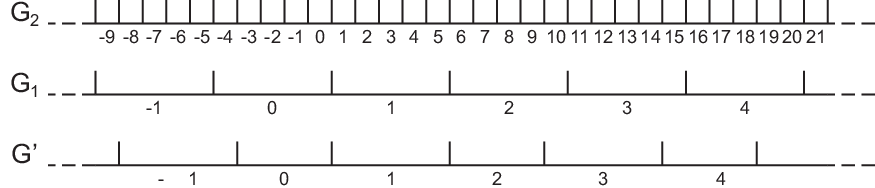
The original definition of altering-tick given by Ning et al. (?) as reported above, has the following problems when an arbitrary negative value for is used: (1) It allows the definition of a that is not a full-integer labeled granularity and (2) It allows the definition of a that does not even satisfy the definition of granularity. In order to avoid this undesired behavior, we impose the following restriction:
where is formally defined by Bettini et al. (?).
Intuitively, represents the minimum distance (in terms of granules of ) between two consecutive granules of .
3.1.3 The Shift Operation
Let be a full-integer labeled granularity, and an integer. The shifting operation generates a new granularity by shifting the labels of by positions. More formally, is the granularity such that for each integer , . Note that is also full-integer labeled.
3.1.4 The Combining Operation
Let and be granularities with label sets and respectively. The combining operation generates a new granularity by combining all the granules of that are included in one granule of into one granule of . More formally, for each , let if , and otherwise let . Then is the granularity with the label set such that for each in , .
As an example, given granularities b-day and month, the granularity for business months can be generated by
3.1.5 The Anchored Grouping Operation
Let and be granularities with label sets and respectively, where is a label-aligned subgranularity of , and is a full-integer labeled granularity. The anchored grouping operation generates a new granularity by combining all the granules of that are between two granules of into one granule of . More formally, is the granularity with the label set such that for each , where is the next label of after .
For example, each academic year at a certain university begins on the last Monday in August, and ends on the day before the beginning of the next academic year. Then, the granularity corresponding to the academic years can be generated by .
3.2 The Granule-Oriented Operations
Differently from the grouping-oriented operations, the granule-oriented operations do not modify the granules of a granularity, but rather enable the selection of the granules that should remain in the new granularity.
3.2.1 The Subset Operation
Let be a granularity with label set , and integers such that . The subset operation generates a new granularity by taking all the granules of whose labels are between and . More formally, is the granularity with the label set , and for each , . For example, given granularity year, all the years in the 20th century can be generated by . Note that is a label-aligned subgranularity of , and is not a full-integer labeled granularity even if is. We also allow the extensions of setting or with semantics properly extended.
3.2.2 The Selecting Operations
The selecting operations are all binary operations. They generate new granularities by selecting granules from the first operand in terms of their relationship with the granules of the second operand. The result is always a label-aligned subgranularity of the first operand granularity.
There are three selecting operations: select-down, select-up and select-by-intersect. To facilitate the description of these operations, the notation is used. Intuitively, if is a set of integers, selects elements starting from the -th one (for a formal description of the operator see (?)).
Select-down operation. For each granule , there exits a set of granules of that is contained in . The operation , where and are integers, selects granules of by using on each set of granules (actually their labels) of that are contained in one granule of . More formally, is the granularity with the label set
and for each , . For example, Thanksgiving days are the fourth Thursdays of all Novembers; if Thursday and November are given, it can be generated by .
Select-up operation. The select-up operation generates a new granularity by selecting the granules of that contain one or more granules of . More formally, is the granularity with the label set
and for each , . For example, given granularities Thanksgiving and week, the weeks that contain Thanksgiving days can be defined by .
Select-by-intersect operation. For each granule , there may exist a set of granules of , each intersecting . The operation, where and are integers, selects granules of by applying operator to all such sets, generating a new granularity . More formally, is the granularity with the label set
and for each , . For example, given granularities week and month, the granularity consisting of the first week of each month (among all the weeks intersecting the month) can be generated by .
3.2.3 The Set Operations
In order to have the set operations as a part of the calendar algebra and to make certain computations easier, we restrict the operand granularities participating in the set operations so that the result of the operation is always a valid granularity: the set operations can be defined on and only if there exists a granularity such that and are both label-aligned subgranularities of . In the following, we describe the union, intersection, and difference operations of and , assuming that they satisfy the requirement.
Union. The union operation generates a new granularity by collecting all the granules from both and . More formally, is the granularity with the label set , and for each ,
For example, given granularities Sunday and Saturday, the granularity of the weekend days can be generated by .
Intersection. The intersection operation generates a new granularity by taking the common granules from both and . More formally, is the granularity with the label set , and for each , (or equivalently ).
Difference. The difference operation generates a new granularity by excluding the granules of from those of . More formally, is the granularity with the label set , and for each , .
4 From Calendar Algebra to Periodical Set
In this section we first describe the overall conversion process and then we report the formulas specific for the conversion of each calendar algebra operation. Finally, we present a procedure for relabeling the resulting granularity, a sketch complexity analysis and some considerations about the period length minimality.
4.1 The Conversion Process
Our final goal is to provide a correct and effective way to convert calendar expressions into periodical representations. Under appropriate limitations, for each calendar algebra operation, if the periodical descriptions of the operand granularities are known, it is possible to compute the periodical characterization of the resulting granularity.
This result allows us to calculate, for any calendar, the periodical description of each granularity in terms of the bottom granularity. In fact, by definition, the bottom granularity is fully characterized; hence it is possible to compute the periodical representation of all the granularities that are obtained from operations applied to the bottom granularity. Recursively, the periodical description of all the granularities can be obtained.
The calendar algebra presented in the previous section can represent all the granularities that are periodical with finite exceptions (i.e., any granularity such that bottom groups periodically with finite exceptions into ). Since with the periodical representations defined in Section 2 it is not possible to express the finite exceptions, we need to restrict the calendar algebra so that it cannot represent them. This implies allowing the Subset operation to be only used as the last step of deriving a granularity. Note that in the calendar algebra presented by Ning et al. (?) there was an extension to the altering-tick operation to allow the usage of as the parameter (i.e., ); the resulting granularity has a single exception hence is not periodic. This extension is disallowed here in order to generate periodical granularities only (without finite exceptions).
The conversion process can be divided into three steps: in the first one the period length and period label distance are computed; in the second we derive the set of labels in one period, and in the last one the composition of the explicit granules is computed. For each operation we identify the correct formulas and algorithms for the three steps.
The first step consists in computing the period length and the period label distance of the resulting granularity. Those values are calculated as a function of the parameters (e.g. the “grouping factor” , in the Group operation) and the operand granularities (actually their period lengths and period label distances).
The second step in the conversion process is the identification of the label set of the resulting granularity. In Section 2.4 we pointed out that in order to fully characterize a granularity it is sufficient to identify the labels in any period of the granularity. In spite of this theoretical result, to perform the computations required by each operation we need the explicit granules of the operand granularities to be “aligned”. There are two possible approaches: the first one consist in computing the explicit granules in any period and then recalculate the needed granules in the correct position in order to eventually align them. The second one consists in aligning all the periods containing the explicit granules with a fixed granule in the bottom granularity. After considering both possibilities, for performance reasons, we decided to adopt the second approach. We decided to use as the “alignment point” for all the granularities. A formal definition of the used formalism follows.
Let be a granularity and be the smallest positive integer such that is defined. We call and the set of labels of contained in . Note that this definition of is an instance of the definition of given in Section 2.4. The definition of provided here is useful for representing and actually the final goal of this step is to compute ; however is not suitable for performing the computations. The problem is that if starts before (i.e., ) then the granule begins at or before , and hence is necessary for the computations; however .
To solve the problem we introduce the symbol to represent the set of all labels of granules of that cover one in . It is easily seen that if does not cover , then , otherwise . Therefore the conversion between and and vice versa is immediate.
The notion of is still not enough to perform the computations. The problem is that when a granularity is used as an operand in an operation, the period length of the resulting granularity is generally bigger than the period length of . Therefore it is necessary to extend the notion of to the period length of using in spite of in the definition of . The symbol used for this notion is .
The idea is that when is used as the operand in an operation that generates , is computed from . This set is then used by the formula that we provide below to compute .
The computation of is performed as follows: if is defined by an operation that returns a full-integer labeled granularity, then it is sufficient to compute the value of . Indeed it is easily seen that . If is defined by any other algebraic operation, we provide the formulas to compute ; from we easily derive .
Example 3
Figure 3 shows granularities , and ; it is clear that and . Moreover, and therefore . Since then . On the other hand, since , then .
Suppose that a granularity has period length ; then and .

The third (and last) step of the conversion process is the computation of the composition of the explicit granules. Once has been computed, it is sufficient to apply, for each label of the formulas presented in Chapter 3.
4.2 Computability Issues
In some of the formulas presented below it is necessary to compute the set of labels of a granularity such that where is a granularity and is a specific label of . Since contains an infinite number of labels, it is not possible to check, if . However it is easily seen that s.t. . Therefore s.t. is defined and .
Therefore we compute the set by considering all the labels of s.t. s.t. and . Since the set is finite33 3 With the calendar algebra it is not possible to define granularities having granules that maps to an infinite set of time instants., the computation can be performed in a finite time. The consideration is analogous if is the set such that or .
4.3 The Group Operation
Proposition 1
If , then:
- 1.
and ;
- 2.
;
- 3.
.
Example 4
Figure 4 shows an example of the group operation: . Since and , then and . Moreover, since , then and therefore and . Finally i.e., .

4.4 The Altering-tick Operation
Proposition 2
If then:
- 1.
and
- 2.
;
- 3.
where and are defined in Section 3.1.2.
Referring to step 2., note that when computing the explicit characterization of the granules of is still unknown. To perform the operation we need to know at least the explicit granules of one of its periods. We choose to compute the granules labeled by . When is derived, the granules labeled by will be computed so that the explicit granules are aligned to as required.
Example 5
Figure 5 shows an example of the altering-tick operation: . Since , , and , then and . Moreover, since , then and therefore and hence . Finally ; analogously we derive , , , and .
4.5 The Shift Operation
Proposition 3
If , then:
- 1.
and ;
- 2.
;
- 3.
.
Example 6
The shifting operation can easily model time differences. Suppose granularity USEast-Hour stands for the hours of US Eastern Time. Since the hours of the US Pacific Time are 3 hours later than those of US Eastern Time, the hours of US Pacific Time can be generated by USPacific-Hour(USEast-Hour).

4.6 The Combining Operation
Proposition 4
Given , then:
- 1.
and ;
- 2.
let be ; then ;
- 3.
.
Example 7
Figure 7 shows an example of the combining operation: . Since , , and , then and . Moreover, since and , then and hence . Since for , then ; moreover, since , then . Finally and ; consequently, i.e., and i.e., .

4.7 The Anchored Grouping Operation
Proposition 5
Given , then:
- 1.
and ;
- 2.
where is the greatest among the labels of that are smaller than .
- 3.
where is the next label of after .
Example 8
Figure 8 shows an example of the anchored grouping operation: the USweek (i.e., a week starting with a Sunday) is defined by the operation Anchored-group(day, Sunday). Since and , then the period length of USweek is 7. Moreover since , and , then . Clearly, since then . Finally, .

4.8 The Subset Operation
The Subset operation only modifies the operand granularity by introducing the bounds. The period length, the period label distance, and the composition of the explicit granules are not affected.
4.9 The Selecting Operations
4.9.1 The Select-down Operation
Proposition 6
Given , then:
- 1.
and ;
- 2.
let
Then
- 3.
.
Example 9
Figure 9 shows an example of the Select-down operation in which granularity is defined as: . Since , and then and . Moreover, since and , then and . Intuitively, , and . Hence and therefore, since , . Finally and .

4.9.2 The Select-up Operation
Proposition 7
Given , then:
- 1.
and ;
- 2.
- 3.
.
Example 10
Figure 10 shows an example of the Select-up operation: . Since , and then and . Moreover, since and , then and . Since , and then and, since , then Finally and .

4.9.3 The Select-by-intersect Operation
Proposition 8
Given , then:
- 1.
and ;
- 2.
then let
then
- 3.
.
Example 11
Figure 11 shows an example of the Select-by-intersect operation in which . Since , and then and . Moreover, since and , then and . Intuitively, , and . Hence and therefore, since , then . Finally and .

4.10 The Set Operations
Since a set operation is valid if the granularities used as argument are both labeled aligned granularity of another granularity, the following property is used.
Proposition 9
If is a labeled aligned subgranularity of , then .
Proposition 10
Given , and , then:
- 1.
and
; - 2.
; ; ;
- 3.
and
Example 12
Figure 12 shows an example of the set operations. Note that both and are labeled aligned subgranularities of . Then , and . Since and then and . Moreover, since and , then , and . Finally , and ; and .

4.11 Relabeling
Granularity processing algorithms are much simpler if restricted to operate on full-integer labeled granularities. Moreover, a further simplification is obtained by using only the positive integers as the set of labels (i.e., ).
In this section we show how to relabel a granularity to obtain a full-integer labeled granularity . A granularity such that can be obtained by using
Note that with the relabeling process some information is lost: for example, if is a labeled aligned subgranularity of and , then, after the relabeling, is not a labeled aligned subgranularity of . The lost information is semantically meaningful in the calendar algebra, and therefore the relabeling must be performed only when the granularity will not be used as an operator in an algebraic operation.
Let be a labeled granularity, and integers with s.t. . The relabeling operation generates a full-integer labeled granularity by relabeling as and relabel the next (and previous) granule of by the next (and previous, respectively) integer. More formally, for each integer , if , then let , and otherwise let where is the -th granule of after (before, respectively) . If the required -th granule of does not exist, then let . Note the is always a full-integer labeled granularity.
The relabeling procedure can be implemented in the periodic representation we adopted by computing the value of . It is easily seen that once is known, the full characterization of can be obtained with: ; and . It is clear that the explicit representation of the granules is not modified.
To compute consider the label ; represents the label of such that is a multiple of . Therefore it is clear that the label s.t. can be computed by . Finally is obtained with where is the distance, in terms of number of granules of , from to .
Example 13
Figure 13 shows an example of the Relabel operation: . Since and then and . Moreover, and . Since and then is the next granule of after . Then and hence . It follows that . Finally and .

The GSTP constraint solver imposes that the first non-empty granule of any granularity ( included) is labeled with . Therefore, when using the relabeling operation for producing granularities for GSTP, the parameter must be set to . The parameter has to be equal to the smallest label among those that identify granules of covering granules of that are all labeled with positive values. By definition of , if ; otherwise is the next label of after .
4.12 Complexity Issues
For each operation the time necessary to perform the three conversion steps, depends on the operation parameters (e.g. the “grouping factor” , in the Group operation) and on the operand granularities (in particular the period length, the period label distance and the number of granules in one period).
A central issue is that if an operand granularity is not the bottom granularity, then its period is a function of the periods of the granularities that are the operands in the operation that defines it. For most of the algebraic operations, in the worst case the period of the resulting granularity is the product of the periods of the operands granularity.
For all operations, the first step in the conversion process can be performed in a constant or logarithmic time. Indeed the formulas necessary to derive the period length and the period label distance involve (i) standard arithmetic operations, (ii) the computation of the Greatest Common Divisor and (iii) the computation of the least common multiple. Part (i) can be computed in a constant time while (ii) and (iii) can be computed in a logarithmic time using Euclid’s algorithm.
For some operations, the second step can be performed in constant time (e.g. Group, Shift or Anchored-group) or in linear time (e.g. set operations). For the other operations it is necessary to compute the set of labels of a granularity such that where is a granularity and (analogously if is the set such that or ). This computation needs to be performed once for each granule . The idea of the algorithm for solving the problem has been presented in Section 4.2. Several optimizations can be applied to that algorithm, but in the worst case (when covers the entire time domain) it is necessary to perform a number of operations linear in the period length of the resulting granularity. If an optimized data structure is used to represent the granularities, the operation can be performed in constant time 44 4 If a non-optimized data structure is used, requires logarithmic time., then the time necessary to perform the second step is linear in the period length of the resulting granularity ().
The last step in the conversion process is performed in linear time with respect to the number of granules in a period of .
The complexity analysis of the conversion of a general algebraic expression needs to consider the composition of the operations and hence their complexity. Finally, relabeling, can be done in linear time.
A more detailed complexity analysis is out of the scope of this work.
5 Minimal Representation and Experimental Results
In this section we address the problem of guaranteeing that the converted representation is minimal in terms of the period length. As we will show in Example 14 the conversion formulas proposed in this paper do not guarantee a minimal representation of the result and it is not clear if conversion formulas ensuring minimality exist. Our approach is to apply a minimization step in the conversion.
The practical applicability of the minimization step depends on the period length of the representation that is to be minimized. Indeed, in our tests we noted that the minimization step is efficient if the conversion formulas proposed in Section 4 are adopted, while it is impractical when the conversion procedure returns a period that is orders of magnitude higher than the minimal one as would be the case if conversion formulas were constructed in a naive way.
5.1 Period Length Minimization
As stated in Section 2, each granularity can have different periodical representations and, for a given granularity, it is possible to identify a set of representations that are minimal i.e. adopting the smallest period length.
Unfortunately, the conversions do not always return a minimal representation, as shown by Example 14.
Example 14
Consider a calendar that has day as the bottom granularity. We can define week as ; by applying the formulas for the Group operation we obtain and .
We can now apply the Altering-tick operation to add one day to every first week every two weeks. Let this granularity be ; applying the formulas for the Altering-tick operation we obtain and .
We can again apply the Altering-tick operation to create a granularity by removing one day from every first granule of every two granules of : . Intuitively, by applying this operation we should get back to the granularity week, however using the formulas for the Altering-tick operation we obtain and ; Hence is not minimal.
In order to qualitatively evaluate how close to the minimal representations the results of our conversions are, we performed a set of tests using an algorithm (?) for minimality checking. In our experimental results the conversions of algebraic expressions defining granularities in real-world calendars, including many user-defined non-standard ones, always returned exactly minimal representations. Non-minimal ones could only be obtained by artificial examples like the one presented in Example 14.
Although a non-minimal result is unlikely in practical calendars, the minimality of the granularity representation is known to greatly affect the performance of the algorithms for granularity processing, e.g., granularity constraint processing (?), calendar calculations (?), workflow temporal support (?). Hence, we considered an extension of the conversion algorithm by adding a minimization step exploiting the technique illustrated by Bettini et al. (?) to derive a minimal representation.
The choice of using only the conversion algorithm or the extended one with minimizations, should probably be driven by performance considerations. In Section 5.3 we report the results of our experiments showing that generally it is advantageous to apply the minimization step. In our implementation, presented in Section 5.2, it is possible to specify if the minimization step should be performed.
5.2 Implementation of the CalendarConverter Web Service
The conversion formulas presented in Section 4 have been implemented into the CalendarConverter web service that converts Calendar Algebra representations into the equivalent periodical ones. More precisely, given a calendar in which granularities are expressed by Calendar Algebra operations, the service converts each operation into an equivalent periodical representation.
The service first rewrites each calendar algebra expression in order to express it only in terms of the bottom granularity. For example, if the bottom granularity is hour, the expression is changed to
Then, Procedure 1 is run for each granularity’s expression. The idea is that the periodical representation of each subexpression is recursively computed starting from the expressions having the bottom granularity as operand. Once each operand of a given operation has been converted to periodical representation, the corresponding formula presented in Section 4 is applied. We call this step the ConvertOperation procedure.
A trivial optimization of Procedure 1 consists in caching the results of the conversions of each subexpression so that it is computed only once, even if the subexpression appears several times (like in the above Monday definition).
- •
Input: a calendar algebra expression ; a boolean value that is set to true if the minimization step is to be executed;
- •
Output: the periodical representation of ;
- •
Method:
5.3 Experimental Results
Our experiments address two main issues: first, we evaluate how the conversion formulas impact on the practical applicability of the conversion procedure and, second, we evaluate how useful is the minimization step.
For the first issue, we execute the conversion procedure with two different sets of conversion formulas and compare the results. The first set is laid out in Section 4. The other, that is less optimized, is taken from the preliminary version of this paper (?).
| Calendar | Section 4 formulas | Less optimized formulas | |||||
|---|---|---|---|---|---|---|---|
| Period | Bot | Conv. | Min. | Tot. | Conv. | Min. | Tot. |
| 1 year | day | 4 | 2 | 6 | 62 | 32 | 94 |
| 4 years | day | 7 | 2 | 9 | 76 | 55 | 131 |
| 1 year | hour | 9 | 2 | 11 | 2,244 | 126,904 | 129,148 |
| 4 years | hour | 16 | 4 | 20 | 4,362 | 908,504 | 912,866 |
| 100 years | day | 127 | 9 | 136 | 3,764 | 1,434,524 | 1,438,288 |
Table 1 shows that when converting calendars having granularities with small minimal period length (first two rows), using the formulas in Section 4 improves the performance by one order of magnitude; However, conversions and minimizations are almost instantaneous with both approaches. On the contrary, when the minimal period length is higher, (last three rows) the time required to minimize the periodical representation is up to five orders of magnitude larger if the formulas proposed by Bettini et al. (?) are used; as a consequence, the entire conversion may require several minutes while, using the formulas presented in Section 4, it still requires only a fraction of a second. If the period length is even larger, the conversion procedure is impractical if the formulas presented by Bettini et al. (?) are used, and indeed in our experiments we did not obtain a result in less than thirteen hours.
For the second issue, we perform a set of three experiments. In the first one we compare the performance of the conversion procedure with the performance of the minimization step. In the experiment we consider the case in which the conversion procedure produces minimal representations. In this case the minimization step is always an overhead since it cannot improve the performance of the conversion procedure.
Figure 14 shows the result of the experiment. Four calendars are considered, each one containing a set of granularities of the Gregorian calendar. The four calendars differs in the values of two parameters: the bottom granularity (it is second for cal-1 and cal-3 while it is minute for cal-2 and cal-4) and the period in which leap years and leap years exceptions are represented (it is , , and years for cal-1, cal-3, cal-2 and cal-4 respectively); As a consequence, the minimal period length of the granularities month and year is about for cal-1, for cal-2, for cal-3 and for cal-4.

As can be observed in Figure 14, the ratio between the time required to perform the conversions and the time required for the minimization step varies significantly from a minimum of for cal-4 to a maximum of for cal-3. The reason is that the complexity of the conversion procedure is mainly affected by the period length of the granularity having the largest period length. On the other hand, the complexity of the minimization step is affected also by other features of the granularities such as their internal structure and the number of integers that can divide at the same time the period label distance, the period length and the number of granules in one period; For more details see (?).
In the second experiment we consider the case in which the conversion procedure produces a non-minimal representation for a granularity in the input calendar; in this case it is possible to benefit from the minimization step. For example, suppose that a granularity is converted and that it is then used as an argument of another Calendar Algebra operation that defines a granularity . The time required to compute the periodical representation of strongly depends on the period length of ; If the period length of is reduced by the execution of the minimization step, the conversion of can be executed faster.
We produced this situation using a technique similar to the one of Example 14; we created Calendar Algebra definitions of the Gregorian calendar in which the granularity day is converted into a granularity having a non-minimal representation. Figure 15 shows the performance obtained converting the same granularities that were used in Figure 14. The difference was that in this case the definition of the granularity day is such that, after the conversion procedure, its period is twice as large as the minimal one (i.e., hours or minutes or seconds depending on the bottom granularity that is used). It can be easily seen that in this case the use of the minimization step can improve the performance of the entire algorithm. Indeed, when the minimization step is performed, the conversion procedure requires about one half of the time that is required when no minimization is performed.

In the third experiment we evaluate the impact of the minimal representation on the performance of applications involving intensive manipulations of granularities. In the test we use the GSTP solver as such an application; it computes solutions of temporal constraints with granularities. A description of the architecture of the GSTP system is provided in Section 6.1.
Figure 16 shows our experiments performed on four temporal constraint networks with granularities. The four networks differs in the number of variables, in the number of constraints and in the granularities used to express the constraints. The networks labeled as “non-minimal” use granularities definitions that are obtained with a technique similar to the one used in Example 14, and have a period that is twice as large as the minimal one.

Figure 16 shows that the use of minimal representations greatly improves the performance of the GSTP solver. Indeed in our experiments the ratio between the time required to solve the network using a non-minimal representation and a minimal one is between three and five. Moreover, the more time required to solve the network, the greater the improvement obtained using the minimal representation; this means that for very complex temporal networks we expect the improvement to be even higher.
Considering the results of our experiments, we conclude that, in general, it is advisable to perform the minimization step. In particular, it is very advantageous in the specific case of GSTP, based on the following considerations: i) the time required to perform the minimization step is only a fraction of the time required to perform the conversion procedure, ii) the conversions are performed off-line in most cases, with respect to granularity processing, and conversion results are cached for future use, and iii) the period length strongly influences the GSTP processing time that is in most cases much longer than the time needed for conversion.
6 Applications
In this section we complement the motivations for this work with a sketch of the applications enabled by the proposed conversion. Firstly we describe the GSTP system, as an example of applications involving intensive manipulation of time granularities. GSTP is used to check the consistency and to find solutions of temporal constraint satisfaction problems with granularities55 5 For a detailed description of the system, see (?).; It has also been applied to check the consistency of inter-organizational workflow models (?). Then, we discuss the use of Calendar Algebra to define new granularities that may later be part of the input of reasoning services, such as GSTP.
6.1 The GSTP System
The GSTP system has been developed at the University of Milan with the objective of providing universal access to the implementation of a set of algorithms for multi-granularity temporal constraint satisfaction (?). It allows the user to specify binary constraints of the form where and are the minimum and maximum values of the distance from to in terms of granularity . Variables take values in the positive integers, and unary constraints can be applied on their domains. For example, the constraint: Event2 should occur 2 to 4 business days after the occurrence of Event1 can be modeled by . This problem is considered an extension of STP (?) to multiple and arbitrary granularities. To our knowledge, GSTP is the only available system to solve this class of temporal constraint satisfaction problems.
Figure 17 shows the general architecture of the GSTP system. There are three main modules: the constraint solver; the web service, which enables external access to the solver; and a user interface that can be used locally or remotely to design and analyze constraint networks.

The constraint solver is the C implementation of the ACG algorithm which has been proposed by Bettini et al. (?), and it runs on a server machine. Following the approach of Bettini et al. (?), the solver uses the representation of granularities based on periodical sets. This representation makes it possible to efficiently compute the core operations on granularities that are required to solve the constraint satisfaction problem. These operations involve, for example, the union and the intersection of periodical sets. While we cannot exclude that these operations may be computed in terms of alternative low level representations, it seems much harder to obtain similar results if a high level representation, such as Calendar Algebra, is used.
The second module of the system is the Web Service that defines, through a WSDL specification, the parameters that can be passed to the constraint solver, including the XML schema for the constraint network specification.

The third module is a remote Java-based user interface, which allows the user to easily edit constraint networks, to submit them to the constraint solver, and to analyze results. In particular, it is possible to have views in terms of specific granularities, to visualize implicit constraints, to browse descriptions of domains, and to obtain a network solution. Fig. 18 shows a screenshot from the interface.
6.2 Defining New Granularities
While the GSTP solver can handle arbitrary granularities, new granularities must be added by editing their explicit periodical representation. This is true in general for any multi-granularity reasoning service based on a low-level representation of granularities, and it is a painful task when the granularities have a large period. For example, in the experimental results illustrated in Figure 16, we used a representation of the granularity month that considers leap years and leap years exceptions in a period of 400 years. In this case, the users have to specify the representation of 4800 granules i.e., the number of months in 400 years.
Because the period length of real world granularities is generally high, a graphical interface does not help if it only supports the user to individually select the explicit granules. An effective solution requires the use of implicit or explicit operations on granules. Among the various proposals, Calendar Algebra provides the richest set of such operators. A question arises: is the definition of granularities in terms of Calendar Algebra really simpler than the specification of the periodical representation? Calendar Algebra does not seem to be user friendly: the exact semantics of each operator may not be immediate for an inexperienced user and some time is required in order to learn how to use each operator.
In practice, we do not think that it is reasonable to ask an unexperienced user to define granularities by writing Calendar Algebra expressions. Nevertheless, we do think that Calendar Algebra can be used by specialized user interfaces to guide the user when specifying granularities. In this sense, we believe that Calendar Algebra plays the same role that SQL does in the definition of databases queries. Similarly to Calendar Algebra, SQL is an abstraction tool that can be directly exploited in all its expressive power by an advanced user, but can also be used by a less experienced user through a graphical user interface, possibly with a reduced expressiveness.
As mentioned above, in the case of periodical representations, graphical user interfaces are not sufficient for making the specification of new granularities practical. On the contrary, in the case of Calendar Algebra, user interfaces can strongly enhance the usability of Calendar Algebra, making its practical use possible also for the definition of involved granularities. There are at least two reasons for this difference. Firstly, the main difficulty of Calendar Algebra is the understanding of the semantics of the operators and the choice of the most appropriate one for a given task. An effective user interface can hide the existence of the algebraic operators to the user showing only how the operators modify existing granularities (i.e., the semantics of the operators). Secondarily, Calendar Algebra allows the compact definition of granularities. This is due to the fact that the Calendar Algebra operations are specifically designed to reflect the intuitive ways in which users define new granularities.
Example 15 shows how a graphical user interface can be effectively used to define a new granularity in terms of Calendar Algebra expression.


Example 15
This example shows how a graphical user interface can be used to support the user in the definition of the granularity final as the set of days, each one corresponding to the last Monday of every academic semester. We assume that the granularities Monday and academicSemester have already been defined. The graphical user interface that we use in this example is a wizard that guides the user step by step. In the first step (Figure 19(a)) the user chooses the kind of operation he wants to perform. In the second step (Figure 19(b)) the user can provide more details about how he wants to modify the operand granularity (Monday, in the example). The results of this choice is a Calendar Algebra expression that is shown in the third step (Figure 19(c)); in this last window the user can also give a name to the granularity that has been defined.
6.3 The Global Architecture

Figure 20 shows a possible architecture for the integration of GSTP, the interface for new granularity definitions and the CalendarConverter web service. A granularity repository collects the Calendar Algebra definitions. Upon request by the GSTP system definitions are converted in low-level representation by the CalendarConverter web service to be efficiently processed. Clearly, caching techniques can be used to optimize the process.
7 Related Work
Several formalisms have been proposed for symbolic representation of granularities and periodicity. Periodicity and its application in the AI and DB area have been extensively investigated (?, ?, ?, ?). Regarding symbolic representation, it is well known the formalism proposed by Leban et al. (?), that is based on the notion of collection, and it is intended to represent temporal expressions occurring in natural language. A collection is a structured set of time intervals where the order of the collection gives a measure of the structure depth: an order 1 collection is an ordered list of intervals, and an order () collection is an ordered list of collections having order . Two operators, called slicing and dicing are used to operate on collections by selecting specific intervals or sub-collections, and by further dividing an interval into a collection, respectively. For example, Weeks:during:January2006 divides the interval corresponding to January2006 into the intervals corresponding to the weeks that are fully contained in that month. This formalism has been adopted with some extensions by many researchers in the AI (?, ?) and Database area (?, ?). In particular, the control statements if-then-else and while have been introduced by Chandra et al. (?) to facilitate the representation of certain sets of intervals. For example, it is possible to specify: the fourth Saturday of April if not an holiday, and the previous business day otherwise.
As for the deductive database community, a second influential proposal is the slice formalism introduced by Niezette et al. (?). A slice denotes a (finite or infinite) set of not necessarily consecutive time intervals. For example, the slice all.Years + {2,4}.Months + {1}.Days 2.Days denotes a set of intervals corresponding to the first 2 days of February and April of each year.
A totally different approach is the calendar algebra described by Ning et al. (?), and considered in this paper. The representation is based on a rich set of algebraic operators on periodic sets as opposed to slicing and dicing over nonconvex intervals.
None of the above cited papers provide a mapping to identify how each operator changes the mathematical characterization of the periodicity of the argument expressions. The problem of finding these mappings is not trivial for some operators.
In (?) the expressive power of the algebras proposed by Leban et al. (?) and Niezette et al. (?) is compared and an extension to the first is proposed in order to capture a larger set of granularities. Since the periodical representation is used to compare expressiveness, a mapping from calendar expressions in those formalisms to periodical representations can be found in the proofs of that paper. However, since minimality is not an issue for the purpose of comparing expressiveness, in many cases the mapping returns non-minimal representations.
Regarding alternative approaches for low-level representation, we already mentioned that the ones based on strings (?) and automata (?, ?) may be considered as an alternative for the target of our conversion. As a matter of fact, an example of the conversion of a Calendar Algebra expression into a string based representation can be found in (?). A complete conversion procedure appeared during the revision process of this paper in the PhD Dissertation by Puppis (?). The aim of the conversion is to prove that the granspecs formalism, used to represent granularities in terms of automata, has at least the same expressiveness as the Calendar Algebra. Hence, obtaining minimal representations was not the goal. Moreover, in their case minimization is not in terms of the period length, but in terms of the automaton size and automaton complexity. About the complexity of reasoning, given an automaton , the worst case time complexity of the operations analogous to our up and down depends linearly on , a value computed from itself and called complexity of . In this sense has the same role of our period length (), even if a precise relationship between the two values is hard to obtain. In our approach we compute up in logarithmic time with respect to and down in linear time with respect to the dimension of the result (that is bounded by ). Other operations, like checking for equivalence, seem to be more complex using automata (?). Techniques for minimization in terms of automaton complexity are presented by Dal Lago et al. (?), and the time complexity is proved to be polynomial, even if the exact bound is not explicitly given. In our approach, the worst case time complexity for the minimization is (?). Overall, the automata approach is very elegant and well-founded, but, on one side it still misses an implementation in order to have some experimental data to compare with, and on the other side only basic operations have been currently defined; it would be interesting to investigate the definition on that formalism of more complex operations like the ones required by GSTP.
8 Conclusion and Future Work
We have presented an hybrid algorithm that interleaves the conversion of Calendar Algebra subexpressions into periodical sets with the minimization of the period length. We have proved that the algorithm returns set-based granularity representations having minimal period length, which is extremely important for the efficiency of operations on granularities. Based on the technical contribution of this paper, a software system is being developed allowing users to access multi-granularity reasoning services by defining arbitrary time granularities with a high-level formalism. Our current efforts are mainly devoted to completing and refining the development of the different modules of the architecture shown in Section 6.3.
As a future work, we intend to develop effective graphical user interfaces to support the definition of Calendar Algebra expressions in a user friendly way. Example 15 described one of the possible interfaces. Another open issue is how to convert a periodical representation of a granularity into a “user friendly” Calendar Algebra expression. This conversion could be useful, for example, to present the result of a computation performed using the periodical representation. However, a naive conversion may not be effective since the resulting calendar algebra expression could be as involved as the periodical representation from which it is derived. For example, a conversion procedure is presented by Bettini et al. (?) to prove that the Calendar Algebra is at least as expressive as the periodical representation; however, the resulting Calendar Algebra expression is composed by a number of Calendar Algebra operations that is linear in the number of granules that are in one period of the original granularity. On the contrary, an effective conversion should generate Calendar Algebra expressions that are compact and easily readable by the user. This problem is somehow related to the discovery of calendar-based association rules (?). Finally, we intend to investigate the usage of the automaton-based representation as a low-level granularity formalism. It would be interesting to know whether, using this representation, it is possible to compute the same operations that can be computed with the periodical representation and if any performance gain could be achieved.
Acknowledgments
We thank the anonymous referees for their useful comments and suggestions. The work of Bettini and Mascetti was partially supported by Italian MIUR InterLink project N.II04C0EC1D. The work of Wang was partially supported by the US NSF grant IIS-0415023.
Appendix A Proofs
A.1 Transitivity of the Periodically Groups Into Relationship
In order to prove the correctness of the conversions of algebraic expressions into periodical sets, it is useful to have a formal result about the transitivity of the periodically groups into relation. In addition to transitivity of , Theorem 1 also says something about period length values.
Theorem 1
Let and be two unbounded granularities such that is periodic in terms of the bottom granularity (i.e., ) and is periodic in terms of (i.e., ). Let and be the period length and the period label distance of in terms of granules of , and the period label distance of in terms of . Then, if for some positive integer , then is periodic in terms of the bottom granularity (i.e., ) and .
Proof.
Since by hypothesis and , if , then . This can be also written as follows:
if
| (1) |
then :
| (2) |
Since , if
| (3) |
then
| (4) |
This can be clearly extended using instead of .
| (5) |
Rewriting (1) substituting according to (3) and rewriting (2) substituting according to (5), we obtain:
if
then
Hence the second condition of Definition 5 is satisfied.
The third one is always satisfied for unbounded granularities.
The first one is satisfied too; in fact since with a period label distance of , then for each label of , is a label of .
Hence, by definition of periodically-groups-into with and .
A.2 Proof of Proposition 1
A.2.1 Part 1
From the definition of the Group operation, for all :
with . Furthermore, :
A.2.2 Part 2
By definition of , we need to show that with .
From the definition of the Group operation, ; hence:
We prove the thesis showing that (1) and that (2) .
(1) Since , hence
(2) First we prove that . Since we have to prove that ; it is equivalent to the inequality that is true since . Since it is trivial that .
A.3 Proof of Proposition 2
A.3.1 Part 1
Proof sketch
We show that with and
then we apply Theorem 1 to obtain the thesis. In
particular we use
and
such that, for each , if , then .
Given an arbitrary granule , we show that is the union of granules that can be obtained by adding to the index of each granule of contained in . Note that since is full-integer labeled. In order to show that this is correct we consider the way granules of are constructed by definition of altering-tick. More precisely, we compute the difference between the label of the first granule of included in and the label of the first granule of included in ; we show that this difference is equal to the difference between the label of the last granule of included in and the label of the last granule of included in . This fact together with the consideration that is a full-integer labeled granularity, leads to the conclusion that and have the same number of granules. It is then clear that the above computed label differences are also equal to the difference between the label of an arbitrary n-th granule of included in and the label of the n-th granule of included in . If this difference is , then we have: if , then . By showing that is a multiple of the thesis follows.
Proof details
Assume and . We need to compute . From the definition of the the altering-tick operation:
and
Note that if , then . Indeed, and, since is a multiple of , then .
Hence, to compute we should consider two cases:
In both cases (again considering the fact that is a multiple of ):
| (19) |
We are left to compute , i.e., the distance in terms of granules of , between and . Since, by hypothesis, and , then the first granule of making and the first granule of making is the same granule. The same can be observed for the first granule of making and the first granule of making . More formally:
and
Hence, we have:
| (20) |
We have shown that the difference between the index of the first granule of making and the index of the first granule of making is equal to the difference between the index of the first granule of making and the index of the first granule of making . Then, we need to compute the difference between the index of the first granule of making and the index of the first granule of making . Since and is a multiple of , for each , if , then . Hence, this difference has value , and for what shown above this is also the value of the difference between the index of the first granule of making and the index of the first granule of making . Then, since with period length and since is a multiple of , we have that, if:
then:
Thus, .
Reconsidering 19:
Analogously we can compute .
Thus, ; hence . Since is a full integer labeled granularity, then and are formed by the same number of granules.
Since we now know and is a multiple of , we have , and . Hence, all the hypothesis of Theorem 1 hold, and its application leads the thesis of this proposition.
A.3.2 Part 2
Since partitions (see table 2.2 of (?)), then (1) is always defined and (2) . Therefore is the label of the granule of that covers the granule of labeled with ; by definition of operation, .
A.4 Proof of Proposition 3
A.4.1 Part 2
By definition of the Shift operation, . Hence .
A.5 Proof of Proposition 4
A.5.1 Part 1
The thesis will follow from the application of Theorem 1. Indeed, we know that and we show that with multiple of . For this we need to identify and s.t., for each , if there exists s.t. , then .
Consider an arbitrary and . By definition of the combining operation, we have and with
and
We now show that is composed by all and only the elements of when the quantity is added. For this purpose we need:
| (21) |
and
| (22) |
A.5.2 Part 2
Let
where ;
We show that by proving that: (1) and (2) .
(1) Suppose by contradiction that exists . Since and since is derived by the Combine operation, then . By definition of the Combine operation ; since , then . Hence (a) .
Moreover, since , then ; therefore . By definition of the Combine operation it is easily seen that . Using this and the previous formula, we derive that (b) .
From (a) and (b) it follows that . We show that this leads to a contradiction.
Since and labels of are contiguous (i.e., s.t. ), then or . We consider the first case, the proof for the second is analogous.
If then (otherwise ).
Let be . Since , then .
If , then contradicting .
If , then and we show that . Indeed, by definition of Combine, . Since we also have ; hence and then .
Since and , then (otherwise ). Therefore, since , then , in contradiction with .
(2) Suppose by contradiction that . Since , by definition of , and ; Therefore, by definition of , .
Since , by definition of , with s.t. . Since , then . By definition of the combine operation, . Moreover, since , by definition of , , contradicting the hypothesis.
A.6 Proof of Proposition 5
A.6.1 Part 1
The thesis will follow from the application of Theorem 1. Indeed, we show that with multiple of . For this we need to identify and s.t., for each , if there exists s.t. , then . Let . By definition of anchored grouping, and where is the first label of after and is the first label of after . By periodicity of , (and since is a multiple of ) the difference between the label of the granule following and the label of the granule following is . More formally, , hence . Then, for each , if , then . By this result and considering , we conclude with . Note that by Proposition 9, , hence is a multiple of . Then, by Theorem 1, we have the thesis.
A.6.2 Part 2
Let
where is the greatest among the labels of that are smaller than . We show that by proving that (1) and (2) .
(1) Suppose by contradiction that . Then, since , then or .
If , then, by definition of , with s.t. . By definition of Anchored-group, where is the first label of after . Therefore . Since is a labeled aligned subgranularity of and since , then and . Hence . It follows that and therefore, by definition of , in contrast with the hypothesis.
If , then, by definition of , . Therefore, since is a labeled aligned subgranularity of ; then with s.t. . Since, by definition of Anchored-group, and since , then . Hence and therefore, by definition of , in contrast with the hypothesis.
(2) Suppose by contradiction that . If then, by definition of , , in contrast with the hypothesis.
If , since s.t. , then or .
If then, by definition of , . Since is a labeled aligned subgranularity of then and hence . Since then in contrast with the hypothesis .
If then, by definition of , or .
If then, let be the next label of after . Since then, by definition , . By definition of then . Since is a labeled aligned subgranularity of then ; therefore . Since and , follows that in contrast with the hypothesis .
Finally if then . Since then with s.t. . Since is the composition of granules of , is defined. Let . By definition of , and therefore . Since, by definition of Anchored-group, is the composition of granules of and since and , then . Therefore since then . It follows that and hence . By definition of , in contrast with the hypothesis.
A.7 Selecting operations
The selecting operations have a common part in the proof for the computation of the period length and the period label distance.
Let be . The proof is divided into two steps: first we show that for each select operation if then (details for Select-down, Select-up and Select-by-intersect operations can be found below). The second step is the application of Theorem 1. Indeed, for each Select operation, the following holds: ; this implies . From step 1 follows that , hence . By this result and considering , we conclude that with which is a multiple of by definition. Then, by Theorem 1 we have the thesis.
A.8 Proof of Proposition 6
A.8.1 Part 1
See Section A.7.
We prove that if then .
By definition of the select-down operation, if then s.t. where is an ordered set defined as follows: . In order to prove the thesis we need to show that . Consider we will note that (this is trivially derived from the periodicity of ). To prove that we show that is obtained from by adding to each of its elements.
Indeed note that from periodicity of , if:
| (25) |
then:
| (26) |
Since , then, from (25), . Moreover, from periodicity of :
| (27) |
Thus is obtained from by adding to each of its elements; therefore if has position in , so has position in . Hence it is trivial that if has position between and in , then has position between and in . Hence if , then .
A.8.2 Part 2
Let
where :
We show that by proving that (1) and (2) .
(1)Suppose by contradiction that . By definition of , ; therefore with s.t. . Moreover, by definition of and by definition of Select-down, hence . Since, by definition of Select-down , then ; hence, by definition of , in contradiction with hypothesis.
(2)Suppose by contradiction that . Since then, by definition of Select-down
therefore, by definition of , .
Since then with s.t. . By definition of Select-down, , then and therefore . Moreover, since , then and therefore . Since , and then, by definition of , , in contrast with the hypothesis.
A.9 Proof of Proposition 7
A.9.1 Part 1
See Section A.7. We prove that if then . From the periodicity of , (this is trivially derived from the periodicity of ). Hence we only need to show that . Since then .
From the periodicity of , if:
| (28) |
then:
| (29) |
Moreover, from the (28) and since :
From the periodicity of :
| (30) |
A.9.2 Part 2
Let
We show that by proving that (1) and (2) .
(1) Suppose by contradiction that . Since , then ; therefore with s. t. . Moreover, by definition of and by definition of Select-down, hence . Since, by definition of Select-up, , then . Hence, by definition of , , in contrast with the hypothesis.
(2) Suppose by contradiction that . Since , then with s.t. . Since, by definition of Select-up, , then ; Therefore, by definition of , . Moreover, since and , by definition of the Select-up operation, then s.t. . Hence by definition of , , in contradiction with hypothesis.
A.10 Proof of Proposition 8
A.10.1 Part 1
See Section A.7. We prove that if , then .
By definition of the select-by-intersect operation, if , then where is an ordered set defined as follows: . In order to prove the thesis we need to show that . Consider note that (this is trivially derived from the periodicity of ). To prove that we show that is obtained from by adding to each of its elements.
Indeed note that if , then . Hence and . From the periodicity of , . From the periodicity of , . So , therefore .
Analogously we can prove that . Hence is obtained from by adding to each of its elements. Therefore, if has position in , then has position in ; hence if has position between and in , then also has position between and in and so .
A.10.2 Part 2
The proof is analogous to the ones of Proposition 6.
A.11 Set Operations
A.11.1 Proof of Proposition 9
Given the periodical granularities H and G with G label aligned subgranularity of H, we prove that . The thesis is proved by considering the common period length of and i.e. .
Let be the difference between the label of the granule of one period of and the label of the granule of the next period, considering as the period length of . Analogously is defined.
By periodicity of , if then ; since is an aligned subranularity of H, and, since is periodic, ; from which we can easily derive that , hence .
From the definition of , s. t. . Moreover, since , then . Therefore .
A.11.2 Property used in the proofs for set operations
Let be and be . Since and are aligned subgranularity of a certain granularity , from Proposition 9 we can easily derive that .
A.12 Proof of Proposition 10
A.12.1 Part 1
Union. Let be and be . The thesis will be proved by showing that if, , then with . Since , two cases will be considered:
- •
. From the periodicity of , ; hence .
- •
. From the periodicity of , ; hence .
Since , then if , then . Hence, by definition of , we have the thesis.
Intersect. . From the periodicity of and , e ; since , then . Moreover ; hence, by the definition of , we have the thesis.
Difference. . Since from the periodicity of . Since , from the periodicity of , (if it would exists , from periodicity of would exists that is not possible for hypothesis). Hence . Moreover ; hence, by the definition of , we have the thesis.
A.12.2 Part 2
Let .
We show that by proving that (1) and (2) .
(1) Suppose by contradiction that . Since then or . Suppose that (the proof is analogous if ). Since , then s.t. . Since, by definition of the Union operation , then . Hence, by definition of , in contrast with the hypothesis.
(2) Suppose by contradiction that . Since , then, by definition of , s.t. . Moreover, by definition of the Union operation, or . Suppose that (the proof is analogous if ). By definition of the Union operation, therefore and so, by definition of , . Hence, by definition of , in contradiction with the hypothesis.
References
- Bettini & Mascetti Bettini, C., & Mascetti, S. (2005). An efficient algorithm for minimizing time granularity periodical representations. In Proc. of the 12th International Symposium on Temporal Representation and Reasoning (TIME), pp. 20–25. IEEE Computer Society.
- Bettini et al. Bettini, C., Mascetti, S., & Pupillo, V. (2005). A system prototype for solving multi-granularity temporal csp. In Recent Advances in Constraints, Revised selected papers from the Workshop on Constraint Solving and Constraint Logic Programming (CSCLP), volume 3419 of Lecture Notes in Computer Science, pp. 142–156. Springer.
- Bettini et al. Bettini, C., Mascetti, S., & Wang., X. S. (2004). Mapping calendar expressions into periodical granularities. In Proc. of the 11th International Symposium on Temporal Representation and Reasoning (TIME), pp. 96–102. IEEE Computer Society.
- Bettini & Sibi Bettini, C., & Sibi, R. D. (2000). Symbolic representation of user-defined time granularities. Annals of Mathematics and Artificial Intelligence, 30(1-4), 53–92.
- Bettini et al. Bettini, C., Wang, X. S., & Jajodia, S. (2000). Time Granularities in Databases, Data Mining, and Temporal Reasoning. Springer.
- Bettini et al. Bettini, C., Wang, X. S., & Jajodia, S. (2002a). Solving multi-granularity temporal constraint networks. Artificial Intelligence, 140(1/2), 107–152.
- Bettini et al. Bettini, C., Wang, X. S., & Jajodia, S. (2002b). Temporal reasoning in workflow systems. Distributed and Parallel Databases, 11(3), 269–306.
- Bresolin et al. Bresolin, D., Montanari, A., & Puppis, G. (2004). Time granularities and ultimately periodic automata. In Proc. of the 9th European Conference on Logics in Artificial Intelligence (JELIA) volume 3229 of Lecture Notes in Computer Science, pp. 513–525. Springer.
- Chandra et al. Chandra, R., Segev, A., & Stonebraker, M. (1994). Implementing calendars and temporal rules in next generation databases. In Proc. of the 10th International Conference on Data Engineering (ICDE), pp. 264–273. IEEE Computer Society.
- Combi et al. Combi, C., Franceschet, M., & Peron, A. (2004). Representing and reasoning about temporal granularities. Journal of Logic and Computation, 14(1), 51–77.
- Combi & Pozzi Combi, C., & Pozzi, G. (2003). Temporal conceptual modelling of workflows. In Proc. of the 22nd International Conference on Conceptual Modeling (ER) volume 2813 of Lecture Notes in Computer Science, pp. 59–76. Springer.
- Cukierman & Delgrande Cukierman, D., & Delgrande, J. P. (1998). Expressing time intervals and repetition within a formalization of calendars. Computational Intelligence, 14, 563–597.
- Dal Lago & Montanari Dal Lago, U., & Montanari, A. (2001). Calendars, time granularities, and automata. In Proc. of the 7th International Symposium on Spatial and Temporal Databases (SSTD), volume 2121 of Lecture Notes in Computer Science, pp. 279–298. Springer.
- Dal Lago et al. Dal Lago, U., Montanari, A., & Puppis, G. (2003). Towards compact and tractable automaton-based representations of time granularities. In Proc. of the 8th Italian Conference on Theoretical Computer Science (ICTCS), volume 2841 of Lecture Notes in Computer Science, pp. 72–85. Springer.
- Dechter et al. Dechter, R., Meiri, I., & Pearl, J. (1991). Temporal constraint networks. Artificial Intelligence, 49(1-3), 61–95.
- Kabanza et al. Kabanza, F., Stevenne, J. M., & Wolper, P. (1990). Handling infinite temporal data. In Proc. of the 9th ACM SIGACT-SIGMOD-SIGART Symposium on Principles of Database Systems (PODS), pp. 392–403. ACM Press.
- Koomen Koomen, J. (1991). Reasoning about recurrence. International Journal of Intelligent Systems, 6, 461–496.
- Ladkin Ladkin, P. B. (1986). Primitives and units for time specification. In Proc. of the 5th National Conference on Artificial Intelligence (AAAI), pp. 353–359. Morgan Kaufmann.
- Leban et al. Leban, B., McDonald, D., & Forster, D. (1986). A representation for collections of temporal intervals. In Proc. of the 5th National Conference on Artificial Intelligence (AAAI), pp. 367–371. Morgan Kaufmann.
- Li et al. Li, Y., Ning, P., Wang, X. S., & Jajodia, S. (2001). Discovering calendar-based temporal association rules. In Proc. of the 8th International Symposium on Temporal Representation and Reasoning (TIME), pp. 111–118. IEEE Computer Society.
- Montanari Montanari, A. (1996). Metric and Layered Temporal Logic for Time Granularity. Ph.D. thesis, ILLC Dissertation Series 1996-02, University of Amsterdam.
- Morris et al. Morris, R., Shoaff, W., & Khatib, L. (1996). Domain-independent temporal reasoning with recurring events. Computational Intelligence, 12, 450–477.
- Niezette & Stevenne Niezette, M., & Stevenne, J. M. (1992). An efficient symbolic representation of periodic time. In Proc. of the first International Conference on Information and Knowledge Management (CIKM) volume 725 of Lecture Notes in Computer Science, pp. 161–168. Springer.
- Ning et al. Ning, P., Wang, X. S., & Jajodia, S. (2002). An algebraic representation of calendars. Annals of Mathematics and Artificial Intelligence, 36(1-2), 5–38.
- Puppis Puppis, G. (2006). Automata for Branching and Layered Temporal Structures. Ph.D. thesis, Università degli Studi di Udine.
- Terenziani Terenziani, P. (2003). Symbolic user-defined periodicity in temporal relational databases. IEEE Transactions of Knowledge and Data Engineering, 15(2), 489–509.
- Tuzhilin & Clifford Tuzhilin, A., & Clifford, J. (1995). On periodicity in temporal databases. Information Systems, 20(8), 619–639.
- Urgun et al. Urgun, B., Dyreson, C. E., Snodgrass, R. T., Miller, J. K., Soo, M. D., Kline, N., & Jensen, C. S. (2007). Integrating multiple calendars using TauZaman. Software-Practice Experience, to appear.
- Wijsen Wijsen, J. (2000). A string-based model for infinite granularities. In Spatial and Temporal Granularity: Papers from the AAAI Workshop. Technical Report WS-00-08, pp. 9–16. AAAI Press.