Acceleration of Uncertainty Updating in the Description of Transport Processes in Heterogeneous Materials

Durability of structures is influenced by moisture damage processes. High moisture levels cause metal corrosion, wood decay and other structural degradation. Thermal expansion and contraction, on the other hand, can induce large displacements and extensive damage to structural materials with differing coefficients ,e.g. masonry. The Charles Bridge in Prague, currently the subject of rehabilitation works, is a typical example, see [1]. A study of the coupled heat and moisture transport behaviour is thus essential in order to improve the building materials’ performance. So far, a vast number of models have been introduced for the description of transport phenomena in porous media. An extensive overview of transport models can be found in [2]. In this work we focus on the model by Künzel [3], since the predicted results comply well with the results of experimental measurements [4], once the relevant material parameters are well estimated.

Material properties are usually determined from experimental measurements via an identification procedure, see e.g. [5]. However, the experimental measurements as well as the identification methods involve some inevitable errors. Bayesian updating, employed within this study, provides a general framework for inference from noisy and limited data. It enables mutually involving both expert knowledge of the material, such as limit values of physical parameters, and information from experimental observations and measurements. In other words, it uses experimental data to update the so-called a priori uncertainty in the material description and results in a posterior probabilistic description of material performance [6]. In addition, unlike traditional identification techniques that aim to regularise the ill-posed inverse problem to achieve a point estimate, the Bayesian identification process leads to a well-posed problem in an expanded stochastic space.

The main disadvantage of Bayesian updating lies in the significant computational effort that results from the sampling-based estimation of posterior densities [7]. While deterministic quadrature or cubature may be attractive alternatives to Monte Carlo at low to moderate dimensions [8], computationally exhaustive Markov chain Monte Carlo (MCMC) remains the most general and flexible method for complex and high-dimensional distributions [9, 10]. In a sampling-based procedure, the posterior distribution must be evaluated for any sample generated from the prior one in order to decide, whether the sample is admissible or not. The computation of the posterior involves the evaluation of the computational model—the FE discretisation of a non-linear partial differential equation (PDE)—relating model (i.e. material) parameters and observable quantities (i.e. model outputs). Hence, complex and time-consuming models can make the sampling procedure practically unfeasible.

Bayesian updating of uncertainty in the description of the parameters of Künzel’s model is thoroughly described in [11] for the case of heterogeneous material, where material parameters are described by random fields (RFs). It was shown that Bayesian updating is applicable even for such a complex and nonlinear model as Künzel’s model. However, the demonstrated results were performed for a sample with a coarse FE, thereby rendering the evaluation of the numerical model computationally relatively cheap. A higher complexity of modelled structure and its FE-based numerical model lead to time-consuming simulations and are prohibitive for the sampling procedure. In such a case one may construct an approximation of the model response and evaluate this within the sampling procedure in order to render the updating procedure feasible [12, 13].

The efficient forward propagation of uncertainty, which may describe material properties, the geometry of the domain, external loading etc., from model parameters to model outputs is a main topic of stochastic mechanics. The recently developed polynomial chaos (PC) variant of the stochastic finite element method (SFEM)—the spectral SFEM (SSFEM) [14, 15, 16, 17, 18]—has become one of the promising techniques in this area. Some of the uncertainties in the model are represented as random fields/processes. Here one often employed technique in SFEM computations is the use of a truncated Karhunen-Loève expansion (KLE) to represent the RFs in a computationally efficient manner by means of a minimal set of random variables (RVs) [19, 16, 20, 21], via an eigenvalue decomposition of the covariance. This approach involves the introduction of an orthogonal—hence uncorrelated—basis in a space of RVs. These are projections of the RF onto the orthogonal KL eigenfunctions, and in the case of Gaussian RFs consists of Gaussian RVs. In that case they are not only uncorrelated but independent—a computationally very important property [22]. However, the material properties very often cannot be modelled as Gaussian due to crucial constraints such as positive definiteness, boundedness in some interval, etc. In such a case, one has to adopt non-Gaussian models and their corresponding approximations, see [17, 18, 23], often as a non-linear transformation of a Gaussian RF. The orthogonal or uncorrelated RVs alluded to above are not Gaussian in that case, and hence not independent. One then may adopt a pure PC representation of the RF in terms of polynomials of independent Gaussian RVs [14], or—to take advantage of the dimension reduction inherent in the KLE truncation—one uses the PC representation for the orthogonal/uncorrelated non-Gaussian RVs from the KLE [16, 20].

In this paper, we focus on Künzel’s model [24, 3], defined by uncertain positive-definite material parameters, modelled as log-normal RFs according to the maximum entropy principle. Since these RFs are non-Gaussian, their spectral decomposition (KLE) gives a set of uncorrelated but not necessarily independent RVs. To address this problem, we project the RVs onto a PC basis constructed from Hermite polynomials in independent Gaussian RVs as alluded to in the previous paragraph. Such a combined expansion (KL/PC) is then used to represent the RFs as inputs to the FE discretisation of the nonlinear Künzel model. The solution procedure of Galerkin type for this SPDE is chosen in an “intrusive” manner based on analytic computations in the PC/Hermite algebra [20, 25, 26]. This brings huge computational savings in case of small and moderate problem dimensions, but it requires complete knowledge of the model (the FEM system can not be used in black-box fashion).

Once such a representation is propagated through the physical model, one obtains a description of all desired output quantities in terms of simply evaluable functions—in this case polynomials—of known independent Gaussian RVs. This is often called a surrogate model or a response surface.

The paper is organised in the following way. The next Section 2 reviews Künzel’s model. Section 3 is focused on the probabilistic description of heterogeneous material properties where particular material parameters are not spatially constant. Intrusive stochastic Galerkin method for computing coefficients of the PC-based surrogate of outputs of Künzel’s model is developed in Section 4 and the related outcomes a presented in Section 5. Finally, Section 6 presents the Bayesian updating procedure on Künzel’s model with the results summarized in Section 7, and Section 8 concludes.

Künzel [24, 3] derived balance equations describing coupled heat and moisture transport through porous media using the concepts of Krischer and Kiessl. Krischer [27] identified two transport mechanisms for material moisture, one being the vapour diffusion and the other being described as capillary water movement. In other words, he introduced the gradient of partial pressure in air as a driving force for the water vapour transport and the gradient of liquid moisture content as the driving force for the water transport. This model is then extended by Kiessl [28] who introduced the so-called moisture potential $\Phi$ used for unification of the description of moisture transport in the hygroscopic $\varphi\leq 0.9$ and over-hygroscopic $\varphi>0.9$ range (where $\varphi$ is relative humidity). The introduction of the moisture potential brings several advantages, especially very simple expressions for the moisture transport across the interface. On the other hand, the definition of the moisture potential in the over-hygroscopic range was too artificial, and Kiessl introduced it without any theoretical background, see [2].

For the description of simultaneous water and water vapour transport Künzel chose the relative humidity $\varphi$ as the only moisture potential for both the hygroscopic and the over-hygroscopic range. He also divided the over-hygroscopic region into two sub-ranges—the capillary water region and supersaturated region—where different conditions for water and water vapour transport are considered. In comparison with Kiessl’s or Krischer’s model Künzel’s model brings certain simplifications. Nevertheless, the proposed model describes all substantial phenomena and the predicted results comply well with experimentally obtained data [4]. Therefore, it was chosen as a physical basis for the formulation of the probabilistic framework.

Künzel’s model is described by the energy balance equation

and the conservation of mass equation

where the transport coefficients defining the material behaviour are nonlinear functions of structural responses, i.e. the temperature $\theta[^{\circ}\mathrm{C}]$ and moisture $\varphi[-]$ fields. We briefly recall their particular relations [3]:

• 1.

  Thermal conductivity $[\mathrm{Wm}^{-1}\mathrm{K}^{-1}]$:

  $$\lambda=\lambda_{0}\left(1+\frac{b_{\mathrm{tcs}}w_{\mathrm{f}}(b-1)\varphi}{\rho_{\mathrm{s}}(b-\varphi)}\right)\,.$$

  (3)

• 2.

  Evaporation enthalpy of water $[\mathrm{Jkg}^{-1}]$:

  $$h_{\mathrm{v}}=2.5008\cdot 10^{6}\left(\frac{273.15}{\theta+273.15}\right)^{(0.267+3.67\cdot 10^{-4}\theta)}\,.$$

  (4)

• 3.

  Water vapour permeability $[\mathrm{kgm}^{-1}\mathrm{s}^{-1}\mathrm{Pa}^{-1}]$:

  $$\delta_{\mathrm{p}}=\frac{1.9446\cdot 10^{-12}}{\mu}\cdot\left(\theta+273.15\right)^{0.81}\,.$$

  (5)

• 4.

  Water vapour saturation pressure $[\mathrm{Pa}]$:

  $$p_{\mathrm{sat}}=611\exp\left(\frac{17.08\theta}{234.18+\theta}\right)\,.$$

  (6)

• 5.

  Liquid conduction coefficient $[\mathrm{kgm}^{-1}\mathrm{s}^{-1}]$:

  $$D_{\varphi}=3.8\frac{a^{2}}{w_{\mathrm{f}}}\cdot 10^{\frac{3w_{\mathrm{f}}(b-1)\varphi}{(b-\varphi)(w_{\mathrm{f}}-1)}}\cdot\frac{b(b-1)}{(b-\varphi)^{2}}\,.$$

  (7)

• 6.

  Total enthalpy of building material $[\mathrm{Jm}^{-3}]$:

  $$H=\rho_{\mathrm{s}}c_{\mathrm{s}}\theta\,.$$

  (8)

• 7.

  Water content $[\mathrm{kgm}^{-3}]$:

  $$w=w_{\mathrm{f}}\frac{(b-1)\varphi}{b-\varphi}\,.$$

  (9)

A more detailed discussion on the transport coefficients can be found in [3, 29]. Some of them defined by Eqs. (3)–(8) depend on a subset of the material parameters listed in Tab. 1. The approximation factor $b$ appearing in Eqs. (3) and (7) can be determined from the relation:

where $w_{80}$ is the equilibrium water content at $0.8\,\mathrm{[-]}$ relative humidity. Moreover, the free water saturation $w_{\mathrm{f}}$ must always be greater than $w_{80}$. Therefore we introduce the water content increment $\mathrm{d}w_{\mathrm{f}}>0$ and define the free water saturation as

Consequently, $w_{80}$ and $\mathrm{d}w_{\mathrm{f}}$ substitute $b$ and $w_{\mathrm{f}}$ as material parameters to be identified within the updating procedure. Tab. 1 presents the resulting list of $W=8$ material parameters to be identified. As an outcome of such a substitution, all identified parameters should be positive and thus described by log-normal RFs (a priori information) with second order statistics (mean values $\mu_{q}$ and standard deviations $\sigma_{q}$) given in Tab. 1. Those particular values are chosen to correspond to materials used in masonry [30].

The partial differential equations (1) and (2) are discretised in space by standard finite elements. This also goes well with the use of the stochastic Galerkin method for the discretisation in the stochastic space. Performing first only the spatial discretisation, the temperature and moisture fields are spatially approximated as

where $N$ is the number of nodes in FE discretisation, $\phi_{n}(\mathchoice{\displaystyle\boldsymbol{x}}{\textstyle\boldsymbol{x}}{\scriptstyle\boldsymbol{x}}{\scriptscriptstyle\boldsymbol{x}})$ are the shape functions (according to the type of used elements) and $u_{\theta,n}$ and $u_{\varphi,n}$ are the nodal values of temperature field $\theta$ and moisture field $\varphi$, respectively.

Using the approximations Eq. (12) and Eqs. (1), (2), we obtain a set of first order differential equations

where $\mathchoice{\displaystyle\boldsymbol{K}}{\textstyle\boldsymbol{K}}{\scriptstyle\boldsymbol{K}}{\scriptscriptstyle\boldsymbol{K}}(\mathchoice{\displaystyle\boldsymbol{u}}{\textstyle\boldsymbol{u}}{\scriptstyle\boldsymbol{u}}{\scriptscriptstyle\boldsymbol{u}})$ is the conductivity matrix, $\mathchoice{\displaystyle\boldsymbol{C}}{\textstyle\boldsymbol{C}}{\scriptstyle\boldsymbol{C}}{\scriptscriptstyle\boldsymbol{C}}(\mathchoice{\displaystyle\boldsymbol{u}}{\textstyle\boldsymbol{u}}{\scriptstyle\boldsymbol{u}}{\scriptscriptstyle\boldsymbol{u}})$ is the capacity matrix, $\mathchoice{\displaystyle\boldsymbol{u}}{\textstyle\boldsymbol{u}}{\scriptstyle\boldsymbol{u}}{\scriptscriptstyle\boldsymbol{u}}^{\mathrm{T}}=(u_{\theta,1},\dots,u_{\theta,N},u_{\varphi,1},\dots,u_{\varphi,N})$ is the vector of nodal values, and $\mathchoice{\displaystyle\boldsymbol{F}}{\textstyle\boldsymbol{F}}{\scriptstyle\boldsymbol{F}}{\scriptscriptstyle\boldsymbol{F}}$ is the vector of prescribed fluxes transformed into nodes. For a detailed formulation of the matrices $\mathchoice{\displaystyle\boldsymbol{K}}{\textstyle\boldsymbol{K}}{\scriptstyle\boldsymbol{K}}{\scriptscriptstyle\boldsymbol{K}}(\mathchoice{\displaystyle\boldsymbol{u}}{\textstyle\boldsymbol{u}}{\scriptstyle\boldsymbol{u}}{\scriptscriptstyle\boldsymbol{u}})$ and $\mathchoice{\displaystyle\boldsymbol{C}}{\textstyle\boldsymbol{C}}{\scriptstyle\boldsymbol{C}}{\scriptscriptstyle\boldsymbol{C}}(\mathchoice{\displaystyle\boldsymbol{u}}{\textstyle\boldsymbol{u}}{\scriptstyle\boldsymbol{u}}{\scriptscriptstyle\boldsymbol{u}})$ and the vector $\mathchoice{\displaystyle\boldsymbol{F}}{\textstyle\boldsymbol{F}}{\scriptstyle\boldsymbol{F}}{\scriptscriptstyle\boldsymbol{F}}$, we refer the interested reader to the doctoral thesis [31, Chapter 3.1].

The numerical solution of the system Eq. (13) is based on a simple temporal finite difference discretisation. If we use time steps $\Delta\tau$ and denote the quantities at time step $i$ with a corresponding superscript, the time-stepping equation is

where $\gamma$ is a generalised midpoint integration rule parameter. In the results presented in this paper the Crank-Nicolson (trapezoidal rule) integration scheme with $\gamma=0.5$ was used. Expressing $\dot{\mathchoice{\displaystyle\boldsymbol{u}}{\textstyle\boldsymbol{u}}{\scriptstyle\boldsymbol{u}}{\scriptscriptstyle\boldsymbol{u}}}^{i+1}$ from Eq. (14) and substituting into the Eq. (13), one obtains a system of non-linear equations:

which can be solved by some iterative method such as Newton-Raphson. For clarification and easier reading, we rewrite Eq. (15) using the symbols $\mathchoice{\displaystyle\boldsymbol{A}}{\textstyle\boldsymbol{A}}{\scriptstyle\boldsymbol{A}}{\scriptscriptstyle\boldsymbol{A}}^{i+1}(\mathchoice{\displaystyle\boldsymbol{u}}{\textstyle\boldsymbol{u}}{\scriptstyle\boldsymbol{u}}{\scriptscriptstyle\boldsymbol{u}}^{i+1}):=\gamma\Delta\tau\mathchoice{\displaystyle\boldsymbol{K}}{\textstyle\boldsymbol{K}}{\scriptstyle\boldsymbol{K}}{\scriptscriptstyle\boldsymbol{K}}^{i+1}(\mathchoice{\displaystyle\boldsymbol{u}}{\textstyle\boldsymbol{u}}{\scriptstyle\boldsymbol{u}}{\scriptscriptstyle\boldsymbol{u}}^{i+1})+\mathchoice{\displaystyle\boldsymbol{C}}{\textstyle\boldsymbol{C}}{\scriptstyle\boldsymbol{C}}{\scriptscriptstyle\boldsymbol{C}}^{i+1}(\mathchoice{\displaystyle\boldsymbol{u}}{\textstyle\boldsymbol{u}}{\scriptstyle\boldsymbol{u}}{\scriptscriptstyle\boldsymbol{u}}^{i+1})$ and $\mathchoice{\displaystyle\boldsymbol{f}}{\textstyle\boldsymbol{f}}{\scriptstyle\boldsymbol{f}}{\scriptscriptstyle\boldsymbol{f}}^{i+1}(\mathchoice{\displaystyle\boldsymbol{u}}{\textstyle\boldsymbol{u}}{\scriptstyle\boldsymbol{u}}{\scriptscriptstyle\boldsymbol{u}}^{i+1}):=\gamma\Delta\tau\mathchoice{\displaystyle\boldsymbol{F}}{\textstyle\boldsymbol{F}}{\scriptstyle\boldsymbol{F}}{\scriptscriptstyle\boldsymbol{F}}^{i+1}+\mathchoice{\displaystyle\boldsymbol{C}}{\textstyle\boldsymbol{C}}{\scriptstyle\boldsymbol{C}}{\scriptscriptstyle\boldsymbol{C}}^{i+1}(\mathchoice{\displaystyle\boldsymbol{u}}{\textstyle\boldsymbol{u}}{\scriptstyle\boldsymbol{u}}{\scriptscriptstyle\boldsymbol{u}}^{i+1})[\mathchoice{\displaystyle\boldsymbol{u}}{\textstyle\boldsymbol{u}}{\scriptstyle\boldsymbol{u}}{\scriptscriptstyle\boldsymbol{u}}^{i}+\Delta\tau(1-\gamma)\dot{\mathchoice{\displaystyle\boldsymbol{u}}{\textstyle\boldsymbol{u}}{\scriptstyle\boldsymbol{u}}{\scriptscriptstyle\boldsymbol{u}}}^{i}]$ in the following form

When dealing with heterogeneous material, some material parameters can vary spatially in an uncertain fashion and therefore RFs are suitable for their description. This means that the uncertainty in a particular material parameter $q$ is modelled by defining $q(\mathchoice{\displaystyle\boldsymbol{x}}{\textstyle\boldsymbol{x}}{\scriptstyle\boldsymbol{x}}{\scriptscriptstyle\boldsymbol{x}})$ for each $\mathchoice{\displaystyle\boldsymbol{x}}{\textstyle\boldsymbol{x}}{\scriptstyle\boldsymbol{x}}{\scriptscriptstyle\boldsymbol{x}}\in\mathcal{G}$ as a RV $q(\mathchoice{\displaystyle\boldsymbol{x}}{\textstyle\boldsymbol{x}}{\scriptstyle\boldsymbol{x}}{\scriptscriptstyle\boldsymbol{x}}):\mathit{\Omega}\rightarrow\mathbb{R}$ on a suitable probability space $(\mathit{\Omega},\mathscr{S},\mathbb{P})$ in some bounded admissible region $\mathcal{G}\subset\mathbb{R}^{d}$. As a consequence, $q:\mathcal{G}\times\mathit{\Omega}\rightarrow\mathbb{R}$ is a RF and one may identify $\mathit{\Omega}$ with the set of all possible realisations of $q$. Alternatively, $q(\mathchoice{\displaystyle\boldsymbol{x}}{\textstyle\boldsymbol{x}}{\scriptstyle\boldsymbol{x}}{\scriptscriptstyle\boldsymbol{x}},\omega)$ can be seen as a collection of real-valued RVs indexed by $\mathchoice{\displaystyle\boldsymbol{x}}{\textstyle\boldsymbol{x}}{\scriptstyle\boldsymbol{x}}{\scriptscriptstyle\boldsymbol{x}}\in\mathcal{G}$.

The description of log-normal RFs given in Tab. 1 can be derived from a Gaussian RF $g(\mathchoice{\displaystyle\boldsymbol{x}}{\textstyle\boldsymbol{x}}{\scriptstyle\boldsymbol{x}}{\scriptscriptstyle\boldsymbol{x}},\omega)$, which is defined by its mean

and its covariance

The log-normal RF $q(\mathchoice{\displaystyle\boldsymbol{x}}{\textstyle\boldsymbol{x}}{\scriptstyle\boldsymbol{x}}{\scriptscriptstyle\boldsymbol{x}},\omega)$ can be then obtained by a nonlinear transformation of a zero-mean unit-variance Gaussian RF $g(\mathchoice{\displaystyle\boldsymbol{x}}{\textstyle\boldsymbol{x}}{\scriptstyle\boldsymbol{x}}{\scriptscriptstyle\boldsymbol{x}},\omega)$ [20, 26] as

The statistical moments $\mu_{g}$ and $\sigma_{g}$ of the Gaussian field can be obtained from the statistical moments $\mu_{q}$ and $\sigma_{q}$ given for the log-normally distributed material property according to the following relations [26]:

In numerical computation random fields are first spatially discretised by finite element method (see Eq. (12)) into a finite collection of points $\{{\mathchoice{\displaystyle\boldsymbol{x}}{\textstyle\boldsymbol{x}}{\scriptstyle\boldsymbol{x}}{\scriptscriptstyle\boldsymbol{x}}}^{n}_{i=1}\}\in\mathcal{G}$. Further, the semi-discretised RF are described by a finite—but probably very large—number of RVs $\mathchoice{\displaystyle\boldsymbol{q}}{\textstyle\boldsymbol{q}}{\scriptstyle\boldsymbol{q}}{\scriptscriptstyle\boldsymbol{q}}(\omega)=(q(\mathchoice{\displaystyle\boldsymbol{x}}{\textstyle\boldsymbol{x}}{\scriptstyle\boldsymbol{x}}{\scriptscriptstyle\boldsymbol{x}}_{1},\omega),\dots,q(\mathchoice{\displaystyle\boldsymbol{x}}{\textstyle\boldsymbol{x}}{\scriptstyle\boldsymbol{x}}{\scriptscriptstyle\boldsymbol{x}}_{n},\omega))$, which are usually highly correlated. Large number of RVs is, however, very challenging for the efficient numerical implementation of forward problem, as well as for MCMC identification. As already alluded to previously, the number of RVs can be reduced by the approximation $\hat{\mathchoice{\displaystyle\boldsymbol{g}}{\textstyle\boldsymbol{g}}{\scriptstyle\boldsymbol{g}}{\scriptscriptstyle\boldsymbol{g}}}(\omega)$ of a RF $\mathchoice{\displaystyle\boldsymbol{g}}{\textstyle\boldsymbol{g}}{\scriptstyle\boldsymbol{g}}{\scriptscriptstyle\boldsymbol{g}}(\omega)$ based on a truncated KLE including much smaller number of RVs [20, 13]. Here we use the KLE on the underlying Gaussian field $\mathchoice{\displaystyle\boldsymbol{g}}{\textstyle\boldsymbol{g}}{\scriptstyle\boldsymbol{g}}{\scriptscriptstyle\boldsymbol{g}}(\omega)$, and hence the RVs in the KLE are independent Gaussian RVs, as already indicated above.

The spatial discretisation of a given RF concerns also the discretisation of corresponding covariance function $C_{g}(\mathchoice{\displaystyle\boldsymbol{x}}{\textstyle\boldsymbol{x}}{\scriptstyle\boldsymbol{x}}{\scriptscriptstyle\boldsymbol{x}},\mathchoice{\displaystyle\boldsymbol{x}}{\textstyle\boldsymbol{x}}{\scriptstyle\boldsymbol{x}}{\scriptscriptstyle\boldsymbol{x}}^{\prime})$ into the covariance matrix $\mathchoice{\displaystyle\boldsymbol{C}}{\textstyle\boldsymbol{C}}{\scriptstyle\boldsymbol{C}}{\scriptscriptstyle\boldsymbol{C}}_{g}$ which is symmetric and positive definite [16, 20]. The KLE is based on the spectral decomposition of the covariance matrix $\mathchoice{\displaystyle\boldsymbol{C}}{\textstyle\boldsymbol{C}}{\scriptstyle\boldsymbol{C}}{\scriptscriptstyle\boldsymbol{C}}_{g}$ leading to the solution of a symmetric matrix eigenvalue problem

where $\mathchoice{\displaystyle\boldsymbol{\psi}}{\textstyle\boldsymbol{\psi}}{\scriptstyle\boldsymbol{\psi}}{\scriptscriptstyle\boldsymbol{\psi}}_{i}$ are orthogonal eigenvectors and $\varsigma_{i}^{2}$ are positive eigenvalues ordered in a descending order. The KLE approximation $\hat{\mathchoice{\displaystyle\boldsymbol{g}}{\textstyle\boldsymbol{g}}{\scriptstyle\boldsymbol{g}}{\scriptscriptstyle\boldsymbol{g}}}(\omega)$ of a RF $\mathchoice{\displaystyle\boldsymbol{g}}{\textstyle\boldsymbol{g}}{\scriptstyle\boldsymbol{g}}{\scriptscriptstyle\boldsymbol{g}}(\omega)$ can then be written as

where $\xi_{i}(\omega)=\mathchoice{\displaystyle\boldsymbol{\psi}_{i}}{\textstyle\boldsymbol{\psi}_{i}}{\scriptstyle\boldsymbol{\psi}_{i}}{\scriptscriptstyle\boldsymbol{\psi}_{i}}^{T}(\mathchoice{\displaystyle\boldsymbol{g}}{\textstyle\boldsymbol{g}}{\scriptstyle\boldsymbol{g}}{\scriptscriptstyle\boldsymbol{g}}(\omega)-\mathchoice{\displaystyle\boldsymbol{\mu}}{\textstyle\boldsymbol{\mu}}{\scriptstyle\boldsymbol{\mu}}{\scriptscriptstyle\boldsymbol{\mu}}_{g})/\varsigma_{i}$ are uncorrelated RVs of zero mean and unit variance, and in case that $g(\mathchoice{\displaystyle\boldsymbol{x}}{\textstyle\boldsymbol{x}}{\scriptstyle\boldsymbol{x}}{\scriptscriptstyle\boldsymbol{x}},\omega)$ and hence $\mathchoice{\displaystyle\boldsymbol{g}}{\textstyle\boldsymbol{g}}{\scriptstyle\boldsymbol{g}}{\scriptscriptstyle\boldsymbol{g}}(\omega)$ are Gaussian, then $x_{i}(\omega)$ are Gaussian and independent. The number $M\leq n$—the number of points used for the discretisation of the spatial domain—is chosen such that Eq. (22) gives a good approximation, i.e. captures a high proportion of the total variance. Higher values of $M$ lead to better description of a RF, smaller values imply faster exploration by MCMC. The eigenvalue problem Eq. (21) is usually solved by a Krylov subspace method with a sparse matrix approximation. For large eigenvalue problems, the authors in [32] propose efficient low-rank and data sparse hierarchical matrix techniques. The approximation of a non-Gaussian RF can be then obtained by a nonlinear transformation of the KLE obtained for a Gaussian RF such as in our particular case, where the approximation of a given RF $\hat{\mathchoice{\displaystyle\boldsymbol{q}}{\textstyle\boldsymbol{q}}{\scriptstyle\boldsymbol{q}}{\scriptscriptstyle\boldsymbol{q}}}(\omega)$ is obtained from the Eq. (19) by the substitution of the Gaussian RF $\mathchoice{\displaystyle\boldsymbol{g}}{\textstyle\boldsymbol{g}}{\scriptstyle\boldsymbol{g}}{\scriptscriptstyle\boldsymbol{g}}(\omega)$ by its KLE $\hat{\mathchoice{\displaystyle\boldsymbol{g}}{\textstyle\boldsymbol{g}}{\scriptstyle\boldsymbol{g}}{\scriptscriptstyle\boldsymbol{g}}}(\omega)$.

We assume full spatial correlation among material properties, i.e. spatial fluctuations for all parameters differ only in magnitude. Taking into account a log-normal distribution of the parameters, the final formulation of the RF describing the parameter $q$ then becomes

where the exponential is to be used at each spatial point, i.e. for each component of the vector inside the parentheses. The statistical moments $\mathchoice{\displaystyle\boldsymbol{\mu}}{\textstyle\boldsymbol{\mu}}{\scriptstyle\boldsymbol{\mu}}{\scriptscriptstyle\boldsymbol{\mu}}_{g}$ and $\sigma_{g}$ are derived from the prior mean $\mathchoice{\displaystyle\boldsymbol{\mu}}{\textstyle\boldsymbol{\mu}}{\scriptstyle\boldsymbol{\mu}}{\scriptscriptstyle\boldsymbol{\mu}}_{q}$ and standard deviation $\sigma_{q}$ for each material parameter according to Eq. (20). The eigenvectors $\mathchoice{\displaystyle\boldsymbol{\psi}}{\textstyle\boldsymbol{\psi}}{\scriptstyle\boldsymbol{\psi}}{\scriptscriptstyle\boldsymbol{\psi}}_{i}$ are obtained for the a priori exponential covariance function

where $\mathchoice{\displaystyle\boldsymbol{r}}{\textstyle\boldsymbol{r}}{\scriptstyle\boldsymbol{r}}{\scriptscriptstyle\boldsymbol{r}}=(r_{1},r_{2})=\mathchoice{\displaystyle\boldsymbol{x}}{\textstyle\boldsymbol{x}}{\scriptstyle\boldsymbol{x}}{\scriptscriptstyle\boldsymbol{x}}-\mathchoice{\displaystyle\boldsymbol{x}}{\textstyle\boldsymbol{x}}{\scriptstyle\boldsymbol{x}}{\scriptscriptstyle\boldsymbol{x}}^{\prime}$, and $l_{x_{1}}=0.1$ $\mathrm{[m]}$ and $l_{x_{2}}=0.04$ $\mathrm{[m]}$ are a priori covariance lengths. Determination of correlation lengths is generally not obvious. In material modelling, one possible way is based on image analysis as described in [33]. A numerical study for a differing number of modes $M$ included in the KLE is presented in [11].

While the KLE can be efficiently applied to reduce the number of RVs and thus to accelerate the exploration of the MCMC method in terms of the number of samples, construction of a surrogate of the computational model can be used for a significant acceleration of each sample evaluation. In [12, 13] methods were introduced for accelerating Bayesian inference in this context through the use of stochastic spectral methods to propagate the prior uncertainty through the forward problem. Here we employ the stochastic Galerkin method [15, 16] to construct the surrogate of Künzel’s model based on polynomial chaos expansion (PCE).

According to Eq. (23), all model parameters are characterised by $M$ independent standard Gaussian RVs $\mathchoice{\displaystyle\boldsymbol{\xi}}{\textstyle\boldsymbol{\xi}}{\scriptstyle\boldsymbol{\xi}}{\scriptscriptstyle\boldsymbol{\xi}}(\omega)=[\xi_{1}(\omega),\dots,\xi_{M}(\omega)]$. Hence, the discretised model response $\mathchoice{\displaystyle\boldsymbol{u}}{\textstyle\boldsymbol{u}}{\scriptstyle\boldsymbol{u}}{\scriptscriptstyle\boldsymbol{u}}(\mathchoice{\displaystyle\boldsymbol{\xi}}{\textstyle\boldsymbol{\xi}}{\scriptstyle\boldsymbol{\xi}}{\scriptscriptstyle\boldsymbol{\xi}}(\omega))=\left(\dots,u_{i}(\mathchoice{\displaystyle\boldsymbol{\xi}}{\textstyle\boldsymbol{\xi}}{\scriptstyle\boldsymbol{\xi}}{\scriptscriptstyle\boldsymbol{\xi}}(\omega))\dots\right)^{\mathrm{T}}$ is a random vector which can be expressed in terms of the same RVs $\mathchoice{\displaystyle\boldsymbol{\xi}}{\textstyle\boldsymbol{\xi}}{\scriptstyle\boldsymbol{\xi}}{\scriptscriptstyle\boldsymbol{\xi}}(\omega)$. Since $\mathchoice{\displaystyle\boldsymbol{\xi}}{\textstyle\boldsymbol{\xi}}{\scriptstyle\boldsymbol{\xi}}{\scriptscriptstyle\boldsymbol{\xi}}(\omega)$ are independent standard Gaussian RVs, Wiener’s PCE based on multivariate Hermite polynomials—orthogonal in the Gaussian measure—$\{H_{\alpha}(\mathchoice{\displaystyle\boldsymbol{\xi}}{\textstyle\boldsymbol{\xi}}{\scriptstyle\boldsymbol{\xi}}{\scriptscriptstyle\boldsymbol{\xi}}(\omega))\}_{\alpha\in\mathcal{J}}$ (see [16, 20] for the notation) is the most suitable choice for the approximation $\tilde{\mathchoice{\displaystyle\boldsymbol{u}}{\textstyle\boldsymbol{u}}{\scriptstyle\boldsymbol{u}}{\scriptscriptstyle\boldsymbol{u}}}(\mathchoice{\displaystyle\boldsymbol{\xi}}{\textstyle\boldsymbol{\xi}}{\scriptstyle\boldsymbol{\xi}}{\scriptscriptstyle\boldsymbol{\xi}}(\omega))$ of the model response $\mathchoice{\displaystyle\boldsymbol{u}}{\textstyle\boldsymbol{u}}{\scriptstyle\boldsymbol{u}}{\scriptscriptstyle\boldsymbol{u}}(\mathchoice{\displaystyle\boldsymbol{\xi}}{\textstyle\boldsymbol{\xi}}{\scriptstyle\boldsymbol{\xi}}{\scriptscriptstyle\boldsymbol{\xi}}(\omega))$ [34], and it can be written as

where $\mathchoice{\displaystyle\boldsymbol{u}}{\textstyle\boldsymbol{u}}{\scriptstyle\boldsymbol{u}}{\scriptscriptstyle\boldsymbol{u}}_{\alpha}$ is a vector of PC coefficients and the index set $\mathcal{J}\subset\mathbb{N}_{0}^{(\mathbb{N})}$ is a finite set of non-negative integer sequences with only finitely many non-zero terms, i.e. multi-indices, with cardinality $|\mathcal{J}|=R$. We collect all the PC coefficients in $\mathchoice{\displaystyle\mathbf{u}}{\textstyle\mathbf{u}}{\scriptstyle\mathbf{u}}{\scriptscriptstyle\mathbf{u}}:=[\dots,\mathchoice{\displaystyle\boldsymbol{u}}{\textstyle\boldsymbol{u}}{\scriptstyle\boldsymbol{u}}{\scriptscriptstyle\boldsymbol{u}}_{\alpha},\dots]_{\alpha\in\mathcal{J}}$. Assuming the uncertainty in all material parameters listed in Tab. 1 and consequently in the model response, Eq. (16) can be rewritten as

Substituting the model response $\mathchoice{\displaystyle\boldsymbol{u}}{\textstyle\boldsymbol{u}}{\scriptstyle\boldsymbol{u}}{\scriptscriptstyle\boldsymbol{u}}^{i+1}(\mathchoice{\displaystyle\boldsymbol{\xi}}{\textstyle\boldsymbol{\xi}}{\scriptstyle\boldsymbol{\xi}}{\scriptscriptstyle\boldsymbol{\xi}})$ by its PC approximation $\tilde{\mathchoice{\displaystyle\boldsymbol{u}}{\textstyle\boldsymbol{u}}{\scriptstyle\boldsymbol{u}}{\scriptscriptstyle\boldsymbol{u}}}^{i+1}(\mathchoice{\displaystyle\boldsymbol{\xi}}{\textstyle\boldsymbol{\xi}}{\scriptstyle\boldsymbol{\xi}}{\scriptscriptstyle\boldsymbol{\xi}})$ given in Eq. (25) and applying a Bubnov-Galerkin projection, one requires that the weighted residuals vanish:

where $\tilde{\mathchoice{\displaystyle\boldsymbol{A}}{\textstyle\boldsymbol{A}}{\scriptstyle\boldsymbol{A}}{\scriptscriptstyle\boldsymbol{A}}}^{i+1}(\mathchoice{\displaystyle\boldsymbol{\xi}}{\textstyle\boldsymbol{\xi}}{\scriptstyle\boldsymbol{\xi}}{\scriptscriptstyle\boldsymbol{\xi}}):=\mathchoice{\displaystyle\boldsymbol{A}}{\textstyle\boldsymbol{A}}{\scriptstyle\boldsymbol{A}}{\scriptscriptstyle\boldsymbol{A}}^{i+1}\left(\mathchoice{\displaystyle\boldsymbol{\xi}}{\textstyle\boldsymbol{\xi}}{\scriptstyle\boldsymbol{\xi}}{\scriptscriptstyle\boldsymbol{\xi}};\tilde{\mathchoice{\displaystyle\boldsymbol{u}}{\textstyle\boldsymbol{u}}{\scriptstyle\boldsymbol{u}}{\scriptscriptstyle\boldsymbol{u}}}^{i+1}(\mathchoice{\displaystyle\boldsymbol{\xi}}{\textstyle\boldsymbol{\xi}}{\scriptstyle\boldsymbol{\xi}}{\scriptscriptstyle\boldsymbol{\xi}})\right)$. Eq. (27) together with Eq. (25) leads to

which is a non-linear system of equations of size $N\times R$.

The approximation $\tilde{\mathchoice{\displaystyle\boldsymbol{u}}{\textstyle\boldsymbol{u}}{\scriptstyle\boldsymbol{u}}{\scriptscriptstyle\boldsymbol{u}}}^{i+1}(\mathchoice{\displaystyle\boldsymbol{\xi}}{\textstyle\boldsymbol{\xi}}{\scriptstyle\boldsymbol{\xi}}{\scriptscriptstyle\boldsymbol{\xi}})$ can be represented through its PC coefficients $\mathchoice{\displaystyle\mathbf{u}}{\textstyle\mathbf{u}}{\scriptstyle\mathbf{u}}{\scriptscriptstyle\mathbf{u}}^{i+1}$, and similarly for all other quantities. Denoting the block-matrix $\mathchoice{\displaystyle\mathbf{A}}{\textstyle\mathbf{A}}{\scriptstyle\mathbf{A}}{\scriptscriptstyle\mathbf{A}}^{i+1}(\mathchoice{\displaystyle\mathbf{u}}{\textstyle\mathbf{u}}{\scriptstyle\mathbf{u}}{\scriptscriptstyle\mathbf{u}}^{i+1}):=\left(\mathbb{E}\left(H_{\beta}(\mathchoice{\displaystyle\boldsymbol{\xi}}{\textstyle\boldsymbol{\xi}}{\scriptstyle\boldsymbol{\xi}}{\scriptscriptstyle\boldsymbol{\xi}})\mathchoice{\displaystyle\boldsymbol{A}}{\textstyle\boldsymbol{A}}{\scriptstyle\boldsymbol{A}}{\scriptscriptstyle\boldsymbol{A}}^{i+1}(\mathchoice{\displaystyle\boldsymbol{\xi}}{\textstyle\boldsymbol{\xi}}{\scriptstyle\boldsymbol{\xi}}{\scriptscriptstyle\boldsymbol{\xi}})H_{\alpha}(\mathchoice{\displaystyle\boldsymbol{\xi}}{\textstyle\boldsymbol{\xi}}{\scriptstyle\boldsymbol{\xi}}{\scriptscriptstyle\boldsymbol{\xi}})\right)\right)_{\beta,\alpha\in\mathcal{J}}$, and the right hand side $\mathchoice{\displaystyle\mathbf{f}}{\textstyle\mathbf{f}}{\scriptstyle\mathbf{f}}{\scriptscriptstyle\mathbf{f}}^{i+1}:=(\mathbb{E}(\mathchoice{\displaystyle\boldsymbol{f}}{\textstyle\boldsymbol{f}}{\scriptstyle\boldsymbol{f}}{\scriptscriptstyle\boldsymbol{f}}^{i+1}(\mathchoice{\displaystyle\boldsymbol{\xi}}{\textstyle\boldsymbol{\xi}}{\scriptstyle\boldsymbol{\xi}}{\scriptscriptstyle\boldsymbol{\xi}})H_{\beta}(\mathchoice{\displaystyle\boldsymbol{\xi}}{\textstyle\boldsymbol{\xi}}{\scriptstyle\boldsymbol{\xi}}{\scriptscriptstyle\boldsymbol{\xi}})))_{\beta\in\mathcal{J}}$, the system Eq. (28) may succinctly be written as

The matrix $\mathchoice{\displaystyle\mathbf{A}}{\textstyle\mathbf{A}}{\scriptstyle\mathbf{A}}{\scriptscriptstyle\mathbf{A}}^{i+1}$ has more structure than is displayed here, but this is outside the scope of this paper; see [16, 20] for details and possible computational procedures.

The evaluation of expected values in Eq. (28) can often be performed analytically in intrusive Galerkin procedures—that is their advantage—using the Hermite algebra [20]. In case they are to be computed numerically, they may be approximated by a weighted sum of samples drawn from the prior distributions. To that purpose, one can apply some integration technique: the Monte Carlo (MC) method, the quasi-Monte Carlo (QMC) method, or some quadrature rule, see [20] for a recent review. The latter ones allow to take advantage of a possibly regular behaviour in the stochastic variables and consequently reduce the number of samples. Since the system of equations Eq. (28) can be quite large, the evaluation of the left hand side for each sample of $\mathchoice{\displaystyle\boldsymbol{\xi}}{\textstyle\boldsymbol{\xi}}{\scriptstyle\boldsymbol{\xi}}{\scriptscriptstyle\boldsymbol{\xi}}$ becomes costly. Here we apply a sparse-grid Smolyak quadrature rule [35, 22, 16, 20], sometimes also named hyperbolic cross integration method, which is an efficient alternative for integration over Gaussian RVs.

After solving the system Eq. (29), one has via Eq. (25) a surrogate representation of the model outputs. This model approximation may be evaluated orders of magnitude more quickly than the evaluation containing the full FE simulation.

For an illustration of the described method, we employ the same simple example as in [11] with the two-dimensional rectangular domain discretised by an FE mesh into $N=80$ nodes and $120$ triangular elements. Its geometry together with the specific loading conditions are shown in Fig. 1.

The initial temperature is $\theta_{\mathrm{in}}=14$ [^∘C] and the moisture $\varphi_{\mathrm{in}}=0.5$ [-] in the whole domain. One side of the domain is submitted to exterior loading conditions $\theta_{\mathrm{ext}}=5$ [^∘C] and $\varphi_{\mathrm{ext}}=0.5$ [-], while the opposite side is submitted to interior loading conditions $\theta_{\mathrm{int}}=24$ [^∘C] and $\varphi_{\mathrm{int}}=0.8$ [-]. The solution of the time-dependent problem in Eq. (29) also involves a discretisation of the time domain $\mathcal{T}$ into $T=151$ time steps and hence the PCE-based surrogate model consist of $N\times T=12,080$ PCEs for the temperature, and the same for the moisture.

In order to describe the accuracy of such a surrogate model, let us define the MC estimate of the error expectation $\varepsilon(\mathchoice{\displaystyle\boldsymbol{u}}{\textstyle\boldsymbol{u}}{\scriptstyle\boldsymbol{u}}{\scriptscriptstyle\boldsymbol{u}})$ as a relative difference between two response fields $\mathchoice{\displaystyle\boldsymbol{u}}{\textstyle\boldsymbol{u}}{\scriptstyle\boldsymbol{u}}{\scriptscriptstyle\boldsymbol{u}}^{a}$ and $\mathchoice{\displaystyle\boldsymbol{u}}{\textstyle\boldsymbol{u}}{\scriptstyle\boldsymbol{u}}{\scriptscriptstyle\boldsymbol{u}}^{b}$ over the discretised spatial and time domain as

The quality of a PC-based surrogate model depends on the number $M$ of eigenmodes involved in KLE describing the fields of material properties as well as on the degree of polynomials $P$ used in the expansion Eq. (25)¹¹ 1 We assume the full PC expansion, where number of polynomials $R$ is fully determined by the degree of polynomials $P$ and number of eigenmodes $M$ according to the well-known relation $R=(M+P)!/(M!P!)$..

Figure 2 shows the error estimate $\varepsilon(\mathchoice{\displaystyle\boldsymbol{u}}{\textstyle\boldsymbol{u}}{\scriptstyle\boldsymbol{u}}{\scriptscriptstyle\boldsymbol{u}})$ computed for different numbers of eigenmodes $M$ and for the polynomial order $P=2$ and $P=3$. Here, the response fields $\mathchoice{\displaystyle\boldsymbol{u}}{\textstyle\boldsymbol{u}}{\scriptstyle\boldsymbol{u}}{\scriptscriptstyle\boldsymbol{u}}^{a}$ are computed by the FEM based on one realization of the KLE of the parameter fields (further shortly called FE simulations) and the response fields $\mathchoice{\displaystyle\boldsymbol{u}}{\textstyle\boldsymbol{u}}{\scriptstyle\boldsymbol{u}}{\scriptscriptstyle\boldsymbol{u}}^{b}$ are obtained by evaluation of the constructed PCE in the same sample point. In order to distinguish the portion of error induced by the KL approximation of the parameter fields, the estimate $\varepsilon(\mathchoice{\displaystyle\boldsymbol{u}}{\textstyle\boldsymbol{u}}{\scriptstyle\boldsymbol{u}}{\scriptscriptstyle\boldsymbol{u}})$ is computed once for the FE simulations using all $M=120$ (dashed lines), and once for the FE simulation using the same number of eigenmodes as in the constructed PCE (solid lines). In other words, the solid lines represent the error induced by PC approximation and the difference between the solid and corresponding dashed line quantifies the error induced by the KL approximation of the parameter fields.

Figure 3 represents the same errors $\varepsilon(\mathchoice{\displaystyle\boldsymbol{u}}{\textstyle\boldsymbol{u}}{\scriptstyle\boldsymbol{u}}{\scriptscriptstyle\boldsymbol{u}})$ as Fig. 2, but this time with respect to the computational effort needed for the computation of PC coefficients. Regarding the obtained results, we focus our following computations on the KL approximation of the material parameters including $M=7$ eigenmodes and a PCE of order $P=2$ providing, at reasonable time, sufficiently good approximation of the model response, namely of the temperature field where the errors are more significant.

For a more detailed presentation of the PCE accuracy, Fig. 4 compares the model response in one node of FE mesh (the node No. $1$ at Fig. 5) at the time $t=400[\mathrm{h}]$ obtained by the FE simulation and by the PCE as a function of the first stochastic variable $\xi_{1}$.

In the Bayesian approach to parameter identification, we assume three sources of information and uncertainties which should be taken into account. The first one is the prior knowledge about the model/material parameters $q_{i}(\omega)$ defining the prior density functions. In our particular case, we know that all the identified parameters are positive-definite and the log-normal random fields with the statistical moments given in Tab. 1 are suitable for a description of the prior information. In fact, they are maximum entropy distributions for this case. We describe the material parameters using the KLE which is fully defined by a finite set of standard Gaussian variables $\mathchoice{\displaystyle\boldsymbol{\xi}}{\textstyle\boldsymbol{\xi}}{\scriptstyle\boldsymbol{\xi}}{\scriptscriptstyle\boldsymbol{\xi}}=[\xi_{1}(\omega),\dots,\xi_{M}(\omega)]$ with the probability density function (pdf) $p_{\mathchoice{\displaystyle\boldsymbol{\xi}}{\textstyle\boldsymbol{\xi}}{\scriptstyle\boldsymbol{\xi}}{\scriptscriptstyle\boldsymbol{\xi}}}(\mathchoice{\displaystyle\boldsymbol{\xi}}{\textstyle\boldsymbol{\xi}}{\scriptstyle\boldsymbol{\xi}}{\scriptscriptstyle\boldsymbol{\xi}})$ and thus, the updating procedure can be performed in terms of $\mathchoice{\displaystyle\boldsymbol{\xi}}{\textstyle\boldsymbol{\xi}}{\scriptstyle\boldsymbol{\xi}}{\scriptscriptstyle\boldsymbol{\xi}}$ turning them into non-Gaussian variables.

Other source of information comes from measurements, which are violated by uncertain experimental errors $\epsilon(\bar{\omega})$. Last uncertainty $\bar{\bar{\omega}}$ arises from imperfection of the numerical model, when for example the description of a real system does not include all important phenomena. However, it is a common situation that the imperfection of the system description cannot be distinguished from measurement error $\epsilon$ and the modelling uncertainties $\bar{\bar{\omega}}$ can be hidden inside the measuring error $\epsilon(\bar{\omega})$. Then we can define the pdf $p_{\mathchoice{\displaystyle\boldsymbol{z}}{\textstyle\boldsymbol{z}}{\scriptstyle\boldsymbol{z}}{\scriptscriptstyle\boldsymbol{z}}}(\mathchoice{\displaystyle\boldsymbol{z}}{\textstyle\boldsymbol{z}}{\scriptstyle\boldsymbol{z}}{\scriptscriptstyle\boldsymbol{z}})$ for noisy measurements $\mathchoice{\displaystyle\boldsymbol{z}}{\textstyle\boldsymbol{z}}{\scriptstyle\boldsymbol{z}}{\scriptscriptstyle\boldsymbol{z}}(\bar{\omega})$.

Bayesian update is based on the idea of Bayes’ rule defined for probabilities. Definition of Bayes’ rule for continuous distribution is, however, more problematic and hence [6, Chapter 1.5] derived the posterior state of information $\pi(\mathchoice{\displaystyle\boldsymbol{\xi}}{\textstyle\boldsymbol{\xi}}{\scriptstyle\boldsymbol{\xi}}{\scriptscriptstyle\boldsymbol{\xi}},\mathchoice{\displaystyle\boldsymbol{z}}{\textstyle\boldsymbol{z}}{\scriptstyle\boldsymbol{z}}{\scriptscriptstyle\boldsymbol{z}})$ as a conjunction of all information at hand

where $\kappa$ is a normalization constant.

The posterior state of information defined in the space of model parameters $\mathchoice{\displaystyle\boldsymbol{\xi}}{\textstyle\boldsymbol{\xi}}{\scriptstyle\boldsymbol{\xi}}{\scriptscriptstyle\boldsymbol{\xi}}$ is given by the marginal pdf

where $\mathit{\bar{\Omega}}$ is a set of random elementary events $\bar{\omega}$ and measured data $\mathchoice{\displaystyle\boldsymbol{z}}{\textstyle\boldsymbol{z}}{\scriptstyle\boldsymbol{z}}{\scriptscriptstyle\boldsymbol{z}}$ enters through the likelihood function $L(\mathchoice{\displaystyle\boldsymbol{\xi}}{\textstyle\boldsymbol{\xi}}{\scriptstyle\boldsymbol{\xi}}{\scriptscriptstyle\boldsymbol{\xi}})$, which gives a measure of how good a numerical model is in explaining the data $\mathchoice{\displaystyle\boldsymbol{z}}{\textstyle\boldsymbol{z}}{\scriptstyle\boldsymbol{z}}{\scriptscriptstyle\boldsymbol{z}}$.

The most general way of extracting the information from the posterior density $\pi_{\mathchoice{\displaystyle\boldsymbol{\xi}}{\textstyle\boldsymbol{\xi}}{\scriptstyle\boldsymbol{\xi}}{\scriptscriptstyle\boldsymbol{\xi}}}(\mathchoice{\displaystyle\boldsymbol{\xi}}{\textstyle\boldsymbol{\xi}}{\scriptstyle\boldsymbol{\xi}}{\scriptscriptstyle\boldsymbol{\xi}})$ is based on sampling procedure governed by MCMC method. For more details about this approach to Bayesian updating of uncertainty in description of couple heat and moisture transport we refer to [11]. In this paper, we focus on the comparison of the posterior information obtained from the sampling procedure using directly the computationally exhaustive numerical model (16) on one hand and using the PC approximation of the model (25) on the other hand.

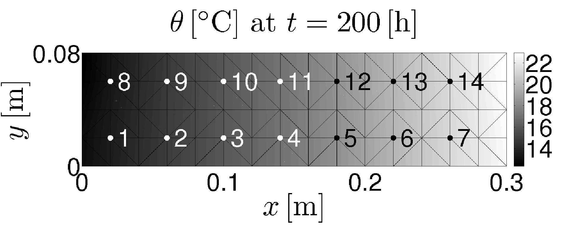
Due to the lack of experimental data, we prepared a virtual experiment using a FE simulation based on parameter fields obtained by the KLE with $7$ eigenmodes so as to avoid the error induced by KLE, which is mainly the subject of the work presented in [11]. A related set of random variables $\mathchoice{\displaystyle\boldsymbol{\xi}}{\textstyle\boldsymbol{\xi}}{\scriptstyle\boldsymbol{\xi}}{\scriptscriptstyle\boldsymbol{\xi}}$ is drawn randomly from the prior distribution and stored for a purpose of latter comparison with the prior and the posterior state of knowledge. The resulting temperature and moisture fields considered as a so-called “true state” or simply the “truth” are shown in Fig. 5. According to [11] the values of temperature and moisture are measured in 14 points (see Figs. 5 (a) and (c)), and at three distinct times (see Figs. 5 (b) and (d)). Hence, the observations $\mathchoice{\displaystyle\boldsymbol{z}}{\textstyle\boldsymbol{z}}{\scriptstyle\boldsymbol{z}}{\scriptscriptstyle\boldsymbol{z}}$ consist of $84$ values.

To keep the presentation of the different numerical aspects of the presented methods clear and transparent, we focus here on a quite common and simple case, where modelling-uncertainties are neglected and measurement errors are assumed to be Gaussian. Then the likelihood function takes the form

where $\mathchoice{\displaystyle\boldsymbol{Y}}{\textstyle\boldsymbol{Y}}{\scriptstyle\boldsymbol{Y}}{\scriptscriptstyle\boldsymbol{Y}}(\mathchoice{\displaystyle\boldsymbol{\xi}}{\textstyle\boldsymbol{\xi}}{\scriptstyle\boldsymbol{\xi}}{\scriptscriptstyle\boldsymbol{\xi}})$ is an observation operator mapping the model response $\mathchoice{\displaystyle\boldsymbol{u}}{\textstyle\boldsymbol{u}}{\scriptstyle\boldsymbol{u}}{\scriptscriptstyle\boldsymbol{u}}$ given parameters $\mathchoice{\displaystyle\boldsymbol{\xi}}{\textstyle\boldsymbol{\xi}}{\scriptstyle\boldsymbol{\xi}}{\scriptscriptstyle\boldsymbol{\xi}}$ and loading $\mathchoice{\displaystyle\boldsymbol{f}}{\textstyle\boldsymbol{f}}{\scriptstyle\boldsymbol{f}}{\scriptscriptstyle\boldsymbol{f}}$ to observed quantities $\mathchoice{\displaystyle\boldsymbol{z}}{\textstyle\boldsymbol{z}}{\scriptstyle\boldsymbol{z}}{\scriptscriptstyle\boldsymbol{z}}$. $\mathchoice{\displaystyle\mathbf{C}}{\textstyle\mathbf{C}}{\scriptstyle\mathbf{C}}{\scriptscriptstyle\mathbf{C}}_{\mathrm{obs}}$ is a covariance matrix representing the uncertainty in experimental error, which is obtained by perturbing the virtual observations by Gaussian noise with standard deviation for temperature $\sigma_{\theta}=0.2$ $\mathrm{[^{\circ}C]}$ and for moisture $\sigma_{\varphi}=0.02$ $\mathrm{[-]}$ so as to get $100$ virtual as an input for the covariance matrix evaluation. In order to be able to compare the posterior state with the true state also in terms of model parameters $\mathchoice{\displaystyle\boldsymbol{\xi}}{\textstyle\boldsymbol{\xi}}{\scriptstyle\boldsymbol{\xi}}{\scriptscriptstyle\boldsymbol{\xi}}$, we assume an artificial situation where the observed quantities $\mathchoice{\displaystyle\boldsymbol{z}}{\textstyle\boldsymbol{z}}{\scriptstyle\boldsymbol{z}}{\scriptscriptstyle\boldsymbol{z}}$ correspond exactly to the true state of temperature and moisture.

The Bayesian update was performed using Metropolis-Hasting algorithm and $100,000$ samples were generated in order to sample the posterior density (31) over the variables $\mathchoice{\displaystyle\boldsymbol{\xi}}{\textstyle\boldsymbol{\xi}}{\scriptstyle\boldsymbol{\xi}}{\scriptscriptstyle\boldsymbol{\xi}}=(\xi_{1}\dots\xi_{M=7})$. The truth state, prior and posterior pdfs obtained by the FE simulations and using the PCE are plotted in Fig. 6.

One can see that the error induced by PC surrogate of model response are negligible in terms of the resulting posterior densities. Figure 6 also demonstrates the fact that the variables $\mathchoice{\displaystyle\boldsymbol{\xi}}{\textstyle\boldsymbol{\xi}}{\scriptstyle\boldsymbol{\xi}}{\scriptscriptstyle\boldsymbol{\xi}}$ being a priori standard Gaussian should not be a posteriori Gaussian.

During the sampling procedure, we stored also the corresponding values of parameter fields and response fields in order to obtain their posterior state of information.

As a result, Fig. 7 shows the comparison of the truth, and prior and posterior pdfs for two material parameters $\lambda_{0}$ and $\mu$ in the top-right corner FE element, and similarly, Fig. 8 presents pdfs for the temperature and moisture in FE node $7$ at $400[\mathrm{h}]$ (i.e. at the $151$-th time step).

We should note that the similarity of the prior and the posterior pdfs for moisture in Fig. 8 is probably caused by the very slight influence of the studied material parameters to the moisture value or more precisely, the prior standard deviations were very small.

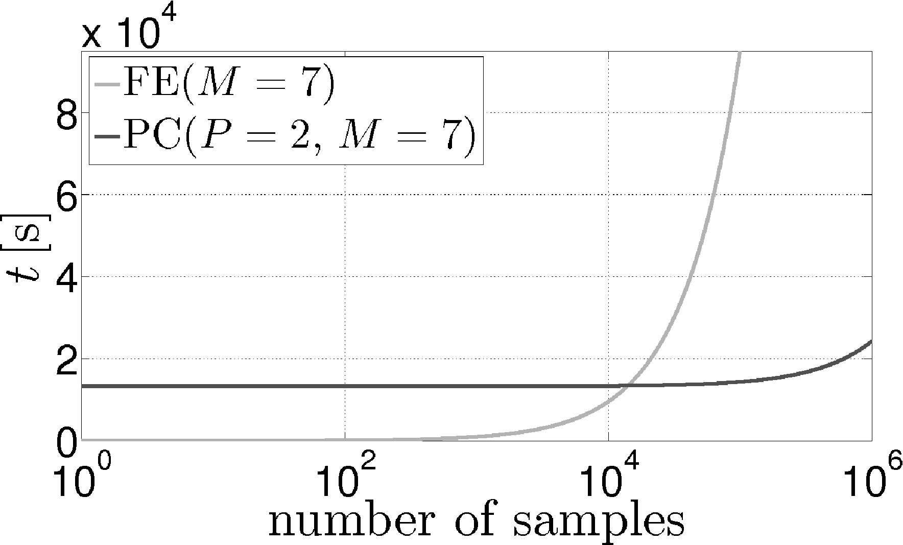
Beside the comparison of the PCE accuracy, we also compared the time necessary to generate the samples. In case of PCE, the total time also includes the time of PC coefficients computation. Particular comparison of computational time needed by FE simulations and by PCE evaluations is demonstrated in Fig. 9.

The presented paper presents an efficient approach to propagation and updating of uncertainties in description of coupled heat and moisture transport in heterogeneous material. In particular, we employed the Künzel’s model, which is sufficiently robust to describe real-world materials, but which is also highly nonlinear, time-dependent and is defined by $8$ material parameters difficult to be estimated from measurements. The updating procedure starts with the prior information about the parameters’ properties such as positive-definitness and second order statistics. Heterogeneity of the material under the study is taken into account by describing the material properties by random fields, which are for a simplicity considered as fully correlated. Then, the corresponding correlation lengths are assume to be known as another a priori information. In order to limit the number of random variables necessary to describe the material, the random fields are approximated by Karhunen-Loève expansion and hence, all the remaining uncertainties are described by a set of standard Gaussian variables whose number is given by the number of eigenmodes involved in KLE.

These uncertainties are then propagated through the numerical model so as to provide a probabilistic characterization of the model response, here the moisture and temperature fields. Simultaneously, the other information including uncertainties coming from the experimental measurements is used to update the prior uncertainties in the model parameters. In order to imitate the experimental measurements, a virtual experiment is prepared together with the relating uncertainties given by a covariance matrix. The Markov Chain Monte Carlo method is then employed so as to sample the posterior state of information.

The primary objective of the presented paper is to accelerate the sampling procedure. To this goal, a polynomial chaos-based approximation of the model response is constructed in order to replace computationally expensive FE simulations by fast evaluations of the PCE during the sampling. In particular, the PC coefficients are obtained by an intrusive stochastic Galerkin method. It is shown that the resulting approximations exhibit high accuracy and the related posterior probability density functions are sufficiently precise as well. Finally, the comparison of the computational effort confirmed the large savings in case of PC evaluations.

While the acceleration obtained by the presented procedure is significant, it can be still unfeasible for very large problems. Our future work will be focused on the elimination of the MCMC sampling procedure itself by the update directly in terms of parameters of probability density functions as proposed in [36].

This outcome has been achieved with the financial support of the Czech Science Foundation, project No. 105/11/0411, the Czech Ministry of Education, Youth and Sports, projects No. MSM6840770003 and No. MEB101105 and the German Research Foundation (DFG) project No. MA 2236/14-1.

References

• [1] J. Zeman, J. Novák, M. Šejnoha, J. Šejnoha, Pragmatic multi-scale and multi-physics analysis of Charles Bridge in Prague, Engineering Structures 30 (11) (2008) 3365–3376.
• [2] R. Černý, P. Rovnaníková, Transport Processes in Concrete, London: Spon Press, 2002.
• [3] H. Künzel, K. Kiessl, Calculation of heat and moisture transfer in exposed building components, International Journal of Heat Mass Transfer 40 (1997) 159–167.
• [4] J. Sýkora, M. Šejnoha, J. Šejnoha, Homogenization of coupled heat and moisture transport in masonry structures including interfaces, Appl. Math. Comput.doi:10.1016/j.amc.2011.02.05.
• [5] A. Kučerová, Identification of nonlinear mechanical model parameters based on softcomputing methods, Ph.D. thesis, Ecole Normale Supérieure de Cachan, Laboratoire de Mécanique et Technologie (2007).
• [6] A. Tarantola, Inverse Problem Theory and Methods for Model Parameter Estimation, Society for Industrial and Applied Mathematics, 2005.
• [7] K. Mosegaard, A. Tarantola, Probabilistic Approach to Inverse Problems, Academic Press, 2002, pp. 237–265.
• [8] M. Evans, T. Swartz, Methods for approximating integrals in statistics with special emphasis on Bayesian integration problems, Statistical Science 10 (3) (1995) 254–272.
• [9] L. Tierney, Markov chains for exploring posterior distributions, Annals of Statistics 22 (4) (1994) 1701–1728.
• [10] W. R. Gilks, S. Richardson, D. Spiegelhalter, Markov Chain Monte Carlo in Practice, Chapman & Hall/CRC, 1995.
• [11] A. Kučerová, J. Sýkora, Uncertainty updating in the description of coupled heat and moisture transport in heterogeneous materials, Appl. Math. Comput.doi:10.1016/j.amc.2011.02.078.
• [12] Y. Marzouk, H. Najm, L. Rahn., Stochastic spectral methods for efficient Bayesian solution of inverse problems, Journal of Computational Physics 224 (2) (2007) 560–586.
• [13] Y. Marzouk, H. Najm, Dimensionality reduction and polynomial chaos acceleration of Bayesian inference in inverse problems, Journal of Computational Physics 228 (6) (2009) 1862–1902.
• [14] R. Ghanem, P. D. Spanos, Stochastic finite elements: A spectral approach, second revised Edition, Dover Publications, Mineola, New York, 2003.
• [15] I. Babuška, R. Tempone, G. E. Zouraris, Galerkin finite element approximations of stochastic elliptic partial differential equations, SIAM Journal on Numerical Analysis 42 (2) (2004) 800–825.
• [16] H. G. Matthies, A. Keese, Galerkin methods for linear and nonlinear elliptic stochastic partial differential equations, Computer Methods in Applied Mechanics and Engineering 194 (12-16) (2005) 1295–1331.
• [17] H. G. Matthies, C. E. Brenner, C. G. Bucher, C. G. Soares, Uncertainties in probabilistic numerical analysis of structures and solids - stochastic finite elements, Structural Safety 19 (3) (1997) 283–336.
• [18] A. Keese, Numerical solution of systems with stochastic uncertainties, Ph.D. thesis, Institute of Scientific Computing, Department of Mathematics and Computer Science, Technische Universität Braunschweig (2004).
• [19] R. Ghanem, Analysis of stochastic systems with discrete elements, Ph.D. thesis, Rice University (1989).
• [20] H. G. Matthies, Encyclopedia of Computational Mechanics, John Wiley & Sons, Ltd., 2007, Ch. Uncertainty Quantification with Stochastic Finite Elements.
• [21] N. Z. Chen, C. G. Soares, Spectral stochastic finite element analysis for laminated composite plates, Computer Methods in Applied Mechanics and Engineering 197 (51–52) (2008) 4830–4839.
• [22] A. Keese, H. G. Matthies, Numerical methods and Smolyak quadrature for nonlinear stochastic partial differential equations, Informatikbericht 2003-5, Institute of Scientific Computing, Department of Mathematics and Computer Science, Technische Universität Braunschweig, Brunswick (2003).
• [23] J.-B. Colliat, M. Hautefeuille, A. Ibrahimbegović, H. G. Matthies, Stochastic approach to size effect in quasi-brittle materials, Comptes Rendus Mécanique 335 (8) (2007) 430–435.
• [24] H. M. Künzel, Simultaneous heat and moisture transport in building components, Tech. rep., Fraunhofer IRB Verlag Stuttgart (1995).
• [25] B. V. Rosić, H. G. Matthies, M. Živkoviić, A. Ibrahimbegović, Stochastic plasticity- a variational and functional approximation approach i: The small strain case, Tech. rep., Institute of Scientific Computing, TU Braunschweig (2011).
• [26] B. Rosić, H. G. Matthies, Computational approaches to inelastic media with uncertain parameters, Journal of the Serbian Society for Computational Mechanics 2 (1) (2008) 28–43.
• [27] O. Krischer, W. Kast, Die wissenschaftlichen Grundlagen der Trocknungstechnik, Dritte Auflage, Berlin: Springer, 1978.
• [28] K. Kiessl, Kapillarer und dampfförmiger Feuchtetransport in mehrschichtlichen Bauteilen, Ph.D. thesis, Universität in Essen (1983).
• [29] R. Černý, J. Maděra, J. Kočí, E. Vejmelková, Heat and moisture transport in porous materials involving cyclic wetting and drying, in: Computational Methods and Experimental Measurements XIV, Vol. 48 of WIT Transactions on Modelling and Simulation, 2009, pp. 3–12.
• [30] Z. Pavlík, J. Mihulka, J. Žumár, R. Černý, Experimental monitoring of moisture transfer across interfaces in brick masonry, in: Structural Faults and Repair, 2010.
• [31] J. Sýkora, Multiscale modeling of transport processes in masonry structures, Ph.D. thesis, Czech Technical University in Prague, Faculty of Civil Engineering, Department of Mechanics (2010).
• [32] B. N. Khoromskij, A. Litvinenko, Data sparse computation of the Karhunen-Loève expansion, in: Proceedings of International Conference on Numerical Analysis and Applied Mathematics 2008, Vol. 1048, 2008, pp. 311–314.
• [33] M. Lombardo, J. Zeman, M. Šejnoha, G. Falsone, Stochastic modeling of chaotic masonry via mesostructural characterization, International Journal for Multiscale Computational Engineering 7 (2) (2009) 171–185.
• [34] D. Xiu, G. E. Karniadakis, The Wiener-Askey polynomial chaos for stochastic differential equations, SIAM J. Sci. Comput. 24 (2) (2002) 619–644.
• [35] S. A. Smolyak, Quadrature and interpolation formulas for tensor products of certain classes of functions, Soviet Math. Dokl. 4 (1963) 240–243.
• [36] B. Rosić, A. Litvinenko, O. Pajonk, H. G. Matthies, Direct bayesian update of polynomial chaos representations, Journal of Computational PhysicsSubmitted for publication.