Asymptotic Freedom in Holographic QCD

Understanding Quantum Chromodynamics (QCD) at the low-energy region has been a challenge for physicists in the past half century. While the high-energy region of QCD is asymptotically free [1] and can be studied and understood well using perturbative method, in the low-energy region, QCD interactions actually become strong and non-linear and cannot be studied perturbatively. Another challenge is to understand the structure of nucleons as the non-linearity of QCD cause the interactions between quarks in the low-energy region to be very complicated.

For the lack of formal derivation, most of the efforts to understand QCD at low-energy region are concentrated in building models that closely resemble QCD at this energy scale, in particular in modeling hadrons. Many models have been proposed in the past, such as Bag Model [2], Constituent Quark Model  [3], Chiral Soliton Model [4], Chiral Lagrangian [5, 6], etc. While most of these models work quite well in the energy region they are prescribed and explain certain properties and behavior of hadrons, they are not derived from first principle. They also generally cannot extend to the high-energy region where QCD works very well.

In 1997 Maldacena conjectured that a certain type of string theory, in particular the type IIB string theory in AdS${}_{5}\times$S₅ corresponds to the conformally invariant large N_c SU(N_c) ${\cal N}=4$ Supersymmetric theory on the 4-dimensional space on the surface of the 5-dimensional AdS space [7]. This is how the moniker AdS/CFT got its name. With this conjecture, the relationship becomes more tangible and a dictionary can be composed to relate parameters and symmetries in one theory to another [8, 9]. Better yet, the two regions of the theory cross where strong coupling, i.e. non-linear region in one theory corresponds to weak coupling, i.e. perturbative region in another theory. To calculate a theory in the strong region all we have to do is to calculate the corresponding theory in the perturbative region. There are two approaches in constructing the dual of QCD, dubbed the top-down and the bottom-up approaches. In the former, one starts from a string theory with an appropriate brane configuration [10, 11, 12]. In the latter, one begins by introducing a 5D action with the few fields needed to reproduce the well-known properties of low-lying QCD states [13, 14, 15]. In this paper we will follow the bottom-up approach.

In its simplest form, the bottom-up models use a 5D AdS metric with cutoff to break conformal symmetry and simulate confinement in QCD. The 5D fields present in the action are bifundamental scalar field $X(x,z)$ and gauge fields, $L(x,z)$ and $R(x,z)$, satisfying the SU$(2)_{\rm L}\times$ SU$(2)_{\rm R}$ symmetry. These 5D fields corresponds to $\bar{q}_{L}q_{R}(x)$, $J_{L}(x)$ and $J_{R}(x)$ operators in the 4D gauge theory respectively. The model produces QCD features quite well [16, 17, 18, 19, 20, 21, 22, 23, 24]. However, the model has some drawbacks. There are ambiguities in the infrared boundary conditions, and the resulting meson spectrum does not satisfy the observed Regge trajectory where the mass squared grows as $n$. Instead, the spectrum of the mass is similar to that of the quantum system of a particle in a box, i.e. $m_{n}^{2}$ grows as $n^{2}$.

Another way to simulate confinement is by introducing a background dilaton field to the 5D action [25]. In order to obtain a meson spectrum that satisfies linear Regge trajectory, the profile of the dilaton field is chosen to be quadratic while the metric of the 5D space remains AdS. However, while the soft-wall model successfully reproduce the linear Regge trajectory, it fails to reproduce a QCD-like chiral symmetry breaking. In particular, in the limit of vanishing quark mass parameter, the quark condensate parameter is vanishing as well. A way to overcome this problem, among other things, was pointed out in [26]. They introduced a quartic term to the bulk scalar potential, included a tachyon field and modified the dilaton profile.

A dilaton field with opposite sign, relative to the one used in [25], has been considered in the literature [27, 28, 29] as it seems to have more appealing confinement properties. In [25] and later reemphasized in [30], this reversed sign choice was discarded because it leads to an unphysical massless vector meson. It was shown that the problem can not be easily remedied unless the asymptotic value of the dilaton field at the IR boundary is changed. With the correct dilaton sign, the wave function of the massless mode is non-normalizable, hence, decouple.

Various aspect of QCD has been investigated using the holographic principle [31, 32, 33, 34, 35, 36, 37, 38, 39, 40, 41]. In this paper, we will use a model introduced in [42] where back reaction by the dilaton field to the AdS metric is considered. Even in the simplest case in which no potential term for the dilaton field presents, the back reaction from the dilaton field automatically provides an IR cutoff. With an addition of appropriate potential terms for the dilaton field, the model can reproduce asymptotic freedom of QCD quite well.

The organization of this paper is as follows. In section 2, we will review the original AdS/QCD proposal for the hard-wall and the soft-wall model. In section 3, we will review the holographic model in [42]. We will discuss the vector part of the action in section 4, and show that the spectrum does not contain massless vector meson. In section 5, we consider the scalar part of the action and investigate the running of the quark mass and the quark condensate. Finally in section 6, we provide the conclusions.

In AdS/CFT there is a correspondence between 5-dimensional fields $\phi(x,z)$, and 4-dimensional operators $\mathcal{O}(x)$ living on the boundary of the 5-dimensional Anti-de Sitter (AdS₅) space, where $z$ is the fifth coordinate. The metric of AdS₅ can be written as

The fifth coordinate, $z$, corresponds to energy scale (or momentum transfer $Q^{2}$), i. e., $z\to 0$ corresponds to infinite energy ($Q^{2}\to\infty$).

The 4D sources in the 4D generating functional $Z_{\rm 4D}[\phi^{0}]$ is called $\phi^{0}(x)$ and the generating functional is defined as follow:

The correspondence maybe written as

where on the right hand side $S_{\rm 5D}[\phi_{cl}]$ is the action evaluated for the classical solution $\phi_{cl}(x,z)$ to the field equations with boundary condition

The constant $\Delta$ depends on the nature of the operator $\mathcal{O}$. Utilizing the correspondence, one obtain the $n$-point correlator

There are an infinite number of 5D fields corresponding to an infinite number of 4D operators in QCD. However, there are only several crucial operators involved in the dynamics of spontaneous chiral symmetry breaking. One of these crucial operators is the quark bilinear $\bar{\psi}_{L}\psi_{R}$, whose non-vanishing vacuum expectation value breaks the full symmetry SU$(N_{f})_{L}\times$SU$(N_{f})_{R}$ down to SU$(N_{f})_{V}$. The corresponding 5D field of the quark bilinear operator is a scalar field, $X$, which transform as a bifundamental. The conserved current operators of the SU$(N_{f})_{L}\times$SU$(N_{f})_{R}$ symmetry, $J^{a\mu}_{L}(x)$ and $J^{b\nu}_{R}(x)$, correspond to the 5D gauge field $L^{a}_{\mu}(x,z)$ and $R^{b}_{\nu}(x,z)$, respectively.

The goal of AdS/QCD is to reproduce a model that resembles QCD as close as possible, including QCD asymptotic freedom behaviour. Following Csaki et. al. formulation [42], we define our action

with $\kappa^{2}$ the 5-dimensional Newton constant and $V(\phi)$ chosen to reproduce asymptotic freedom. Note that $\phi$ is dimensionless here.

We assume QCD gauge coupling is given by $e^{b\phi(z)}$ just like in string theory. For the coupling to run logarithmically we need a solution of the form:

where as usual we have identified the AdS coordinate $z$ with the energy scale and defined $z_{0}=\Lambda^{-1}_{QCD}$. We do not fix the value of $b$ a priori. It is easier to work in coordinate $y$ given by $\exp{(y/R)}\equiv z/R$ in which our solution will take the form: $e^{b\phi(y)}=\frac{R}{y_{0}-y}$. Inverting this we obtain the function for the dilaton

and its derivative

First we write our metric in the $y$ coordinate:

Subtituting the metric into our action we obtain:

Taking the variance of this action with respect to $A$ and $\phi$ and setting it to zero:

Next we use superpotential method by defining a function $W(\phi)$ such that:

Solving for $W(\phi)$ with $\phi^{\prime}$ as defined in Eq. 16, we obtain:

It is very easy to show that the potential is

Now we can solve for the warp factor:

or in $z$ coordinate:

For $e^{-2A(z)}=e^{-2A_{0}}\left(\frac{R}{z}\right)^{2W_{0}R}\left(\log{\frac{z_{0}}{z}}\right)^{\frac{1}{3b^{2}}}$ to resemble AdS metric with $\log z_{0}/z$ factor, we need $A_{0}=0$ and $W_{0}=1/R$. This will give us

and

For the case $b=\pm\sqrt{\frac{2}{3}}$, we got:

and

And finally the metric is

In order to write down the action of the dilaton couple into matter in Einstein frame, we compared the action in string and Einstein frame of a noncritical string theory in 5 dimensions [42]. In string frame the action has the form [45, 46]

The action in Einstein frame is:

where the metric of the string frame and the metric of the Einstein frame are related as $g_{MN}^{str}=e^{\frac{4}{3}\Phi}g_{MN}$. We can rescale the dilaton field to obtain a canonical kinetic term, by using $\Phi=\sqrt{3/8}\phi$.

We have chosen the background dilaton profile such that the model produce asymptotic freedom. Here we will calculate the resulting vector meson spectrum on this background. Using the action in equation (32) and the rescaled dilaton field $\Phi=\sqrt{3/8}\phi$, the vector part of the action can be written as

with the following equation of motion for the bulk-to-boundary propagator of the transverse vector field

where $q$ denotes 4-momentum and $b$ as defined in (14).

In order for the action evaluated on the solution of the equation (34) to be finite when $b>(2/7)\sqrt{2/3}$, the bulk-to-boundary propagator or its derivative must vanish sufficiently fast at the IR boundary. Multiplication of both should vanish sufficiently fast such that the IR surface term of the action vanish.

Evaluating the action on the solution, we obtain

where $P_{T}^{\mu\nu}=(\eta^{\mu\nu}-q^{\mu}q^{\nu}/q^{2})$ and $V^{0}_{\mu}(x)$ is the UV boundary value of the vector field which corresponds to the source of vector current operator. In order to obtain 2-point function for the vector current, one has to take functional derivative with respect to the source $V^{0}_{\mu}$ twice on the 5D action. One obtains from the AdS/CFT correspondence

where we have set the AdS radius to unity ($R=1$). The bulk-to-boundary propagator can be normalized to $V(q,\varepsilon)=1$ at the UV boundary.

The vector meson mass spectrum can be obtained by solving the eigenvalue equation

where $m_{n}$ is the mass of the $n$-th Kaluza Klein modes. The wave function is normalized as follows

The wave functions and their derivatives vanish at both the UV and the IR boundaries, except for the massless mode where the wave function approach a non-zero constant at IR boundary. The vanishing values of the wave functions at the boundaries is crucial for their normalizability.

Setting $m_{0}=0$ in equation (37), one obtains the following solution

which is the upper incomplete gamma function. This function is vanishing at UV boundary and approach $N_{0}\Gamma(1-1/(3b^{2})+7/(6b)\sqrt{3/2})$ at IR boundary. The slope vanishes at the IR boundary for $b>(2/7)\sqrt{2/3}$. The weighting function of the normalization integral is infinite at both UV and IR boundary. However, the vanishing value of $\psi_{0}$ near UV overcome this to make the integrand in (38) goes to zero at the UV boundary. This is not the case at the IR boundary as the wave function goes to a non-zero constant when $b>(2/7)\sqrt{2/3}$. Near the IR boundary, one can pull out $\psi_{0}^{2}$ out of the integral. This leave us with the following integral

which is infinite for $0<b<(7/6)\sqrt{3/2}$, with $\eta$ close to $z_{0}$. In the next section we will show that with $b>0$ the quark mass runs properly, that is, in the high energy limit as the energy scale increases, the quark mass decreases as in QCD.

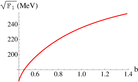
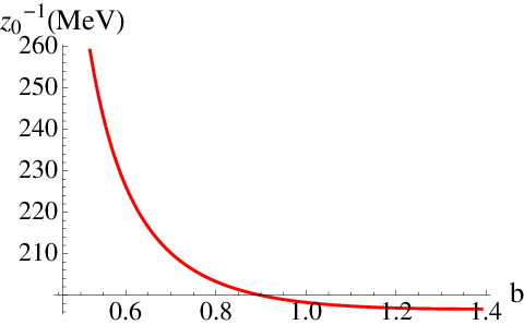
In the case of $b=\sqrt{2/3}$, the first four mass eigenvalues of equation (37) ( in unit of $1/z_{0}$) are $3.83$, $6.52$, $9.14$, $11.74$. We set the value of $z_{0}$ to fit the mass of the first mode to the mass of rho meson. For $m_{\rho}=775.5$ MeV, we obtain $1/z_{0}=202.6$ MeV. The resulting mass of the first few excited states are $1321$ MeV, $1852$ MeV, $2379$ MeV. This mass spectrum grows like $m_{n}^{2}\sim n^{2}$, similar to the hard-wall model. As comparisons, in the original hard-wall model, the corresponding mass of the excited states are $1780$ MeV, $2789$ MeV, $3802$ MeV. For the soft-wall model with quadratic dilaton profile, the corresponding mass are $1097$ MeV, $1343$ MeV, $1551$ MeV.

The bulk-to-boundary propagator can be written as a sum over normalizable modes,

This expansion can be substituted into (36) from which one can identify the decay constant of the vector meson

where $g_{5}=2\pi$ [13]. We obtain $F_{1}=(222\,{\rm MeV})^{2}$. As comparisons, the hard-wall model and the soft-wall model with quadratic dilaton profile yield $F_{1}=(329\,{\rm MeV})^{2}$ and $F_{1}=(260\,{\rm MeV})^{2}$, respectively.

We can vary the value of $b$ while fixing the mass of the lightest vector meson to $775.5$ MeV. The results for the decay constant and the value of $z_{0}^{-1}$ are shown in Figure 1.

The action for dilaton coupled to matter in Einstein frame is:

with $D^{M}X=\partial^{M}X-iA_{L}^{M}X+iXA_{R}^{M}$ and $F_{L,R}^{MN}=\partial^{M}A_{L,R}^{N}-\partial^{N}A_{L,R}^{M}-i[A_{L,R}^{M},A_{L,R}^{N}]$.

The equation of motion for the background field $X_{0}$ in the $u=(y_{0}-y)/R$ coordinate:

where $r=\frac{2}{3b^{2}}-\frac{7}{6b}\sqrt{\frac{3}{2}}$. The solutions of the equation of motion (44) from [47, 48] in terms of Kummer functions are:

with $C_{1}$ and $C_{2}$ are integration constants. Contrary to the soft-wall model, we can keep both terms since the action evaluated on the above solution remains finite.

In order to understand how the scalar field behaves near the UV boundary, we write the solution in the following form, using coordinate transformation $u=-\ln(z/z_{0})$ and Kummer’s transformation [47, 48]

The constants are related as follows

The Kummer’s functions in equation (46) can be written as an infinite series

where $(a)_{n}=(a)(a+1)\ldots(a+n-1)$, and $(a)_{0}=1$. In the limit $z\to 0$ both term in above equation vanish, however, the second term vanish faster than the first term because of the $z^{3}$ factor. Hence, in this limit we can drop the second term and identify the remaining term as quark mass multiplying $\zeta z/2$ as in (8).

We will determine the constants of integration using the value of $m_{q}$ and $\sigma$ at $1/z=2\,\mathrm{GeV}$ from [49] as input parameter. Because the imaginary parts of equation (46) cancel out as a consequence of equation (45) which is real, we take the real part of $X_{0}(z)$ and associate them to the quark mass $m_{q}$ and QCD condensate $\sigma$:

By associating $z_{0}$ with $1/\Lambda_{QCD}$, equation (50) and (51) show how the running of quark mass and QCD condensate as a function of energy scale $1/z=\mu$. Figure (2) shows the running of the quark mass from equation (50) compared with the running of quark mass from perturbative QCD up to two loops calculation [50, 51],

where $\gamma_{0}=2$, $\gamma_{1}=\frac{101}{12}-\frac{5}{18}n_{q}$, $\beta_{0}=11-\frac{2}{3}n_{q}$, $\beta_{1}=51-\frac{19}{3}n_{q}$, and $L=\ln(\mu^{2}/\Lambda^{2})$. Here, $\widetilde{m}_{q}$ is the renormalization group invariant mass.

We vary the value of $r$ while fixing the mass of the lightest vector meson $m_{\rho}=757\,\mathrm{MeV}$. The best fit as shown in figure (2) is for $r=-0.53$ which corresponds to $1/z_{0}=226\,\mathrm{MeV}$ and $\sqrt{F_{\rho}}=197$ MeV.

In figure (3), we fit equation (51) to the one loop QCD calculation for the running of quark condensate in the chiral limit [52, 53]:

with $\gamma_{m}=12/(33-2n_{q})$. The best fit is for $r=-0.29$ which corresponds to $1/z_{0}=259\,\mathrm{MeV}$ and $\sqrt{F_{\rho}}=183$ MeV.

In this paper we have calculated the running of the quark mass and the quark condensate using a dynamical soft-wall model. In order to remove the massless vector meson and to make the quark mass runs properly we have determined the allowed value of parameter $b$ to be $0<b<(7/6)\sqrt{3/2}$. We also find that, contrary to the soft-wall model with quadratic dilaton profile, the model allows for a non-vanishing quark condensate in the chiral limit. We obtain the vector meson mass spectrum similar to that of the hard-wall model. The best fit of this model to the running of the quark mass yield $r=-0.53$, which corresponds to $b=0.60$ and the best fit to the running of the quark condensate yield $r=-0.29$, which corresponds to $b=0.52$.

References

- (1) D. J. Gross and F. Wilczek, ULTRAVIOLET BEHAVIOR OF NON-ABELIAN GAUGE THEORIES, Phys. Rev. Lett. 30 (1973) 1343–1346.
- (2) K. Johnson, QUANTUM CHROMODYNAMICS AND BAG MODEL, . IN *ZUOZ 1985, PROCEEDINGS, STRONG INTERACTIONS* 133-169.
- (3) S. Capstick and N. Isgur, Baryons in a Relativized Quark Model with Chromodynamics, Phys. Rev. D34 (1986) 2809.
- (4) T. H. R. Skyrme, A Unified Field Theory of Mesons and Baryons, Nucl. Phys. 31 (1962) 556–569.
- (5) S. R. Coleman, J. Wess, and B. Zumino, Structure of phenomenological Lagrangians. 1, Phys. Rev. 177 (1969) 2239–2247.
- (6) J. Gasser and H. Leutwyler, Chiral Perturbation Theory to One Loop, Ann. Phys. 158 (1984) 142.
- (7) J. M. Maldacena, The large N limit of superconformal field theories and supergravity, Adv. Theor. Math. Phys. 2 (1998) 231–252, [hep-th/9711200].
- (8) S. S. Gubser, I. R. Klebanov, and A. M. Polyakov, Gauge theory correlators from non-critical string theory, Phys. Lett. B428 (1998) 105–114, [hep-th/9802109].
- (9) E. Witten, Anti-de Sitter space and holography, Adv. Theor. Math. Phys. 2 (1998) 253–291, [hep-th/9802150].
- (10) M. Kruczenski, D. Mateos, R. C. Myers, and D. J. Winters, Towards a holographic dual of large-N(c) QCD, JHEP 05 (2004) 041, [hep-th/0311270].
- (11) T. Sakai and S. Sugimoto, Low energy hadron physics in holographic QCD, Prog. Theor. Phys. 113 (2005) 843–882, [hep-th/0412141].
- (12) T. Sakai and S. Sugimoto, More on a holographic dual of QCD, Prog. Theor. Phys. 114 (2005) 1083–1118, [hep-th/0507073].
- (13) J. Erlich, E. Katz, D. T. Son, and M. A. Stephanov, QCD and a Holographic Model of Hadrons, Phys. Rev. Lett. 95 (2005) 261602, [hep-ph/0501128].
- (14) L. Da Rold and A. Pomarol, Chiral symmetry breaking from five dimensional spaces, Nucl. Phys. B721 (2005) 79–97, [hep-ph/0501218].
- (15) J. Hirn and V. Sanz, Interpolating between low and high energy QCD via a 5D Yang-Mills model, JHEP 12 (2005) 030, [hep-ph/0507049].
- (16) H. R. Grigoryan and A. V. Radyushkin, Form Factors and Wave Functions of Vector Mesons in Holographic QCD, Phys. Lett. B650 (2007) 421–427, [hep-ph/0703069].
- (17) H. J. Kwee and R. F. Lebed, Pion Form Factors in Holographic QCD, JHEP 01 (2008) 027, [arXiv:0708.4054].
- (18) H. R. Grigoryan and A. V. Radyushkin, Pion Form Factor in Chiral Limit of Hard-Wall AdS/QCD Model, Phys. Rev. D76 (2007) 115007, [arXiv:0709.0500].
- (19) H. J. Kwee and R. F. Lebed, Pion Form Factor in Improved Holographic QCD Backgrounds, Phys. Rev. D77 (2008) 115007, [arXiv:0712.1811].
- (20) J. Erlich, Recent Results in AdS/QCD, PoS CONFINEMENT8 (2008) 032, [arXiv:0812.4976].
- (21) Z. Abidin and C. E. Carlson, Gravitational Form Factors of Vector Mesons in an AdS/QCD Model, Phys. Rev. D77 (2008) 095007, [arXiv:0801.3839].
- (22) Z. Abidin and C. E. Carlson, Gravitational Form Factors in the Axial Sector from an AdS/QCD Model, Phys. Rev. D77 (2008) 115021, [arXiv:0804.0214].
- (23) Z. Abidin and C. E. Carlson, Strange hadrons and kaon-to-pion transition form factors from holography, Phys. Rev. D80 (2009) 115010, [arXiv:0908.2452].
- (24) J. Erlich, How Well Does AdS/QCD Describe QCD?, Int. J. Mod. Phys. A25 (2010) 411–421, [arXiv:0908.0312].
- (25) A. Karch, E. Katz, D. T. Son, and M. A. Stephanov, Linear Confinement and AdS/QCD, Phys. Rev. D74 (2006) 015005, [hep-ph/0602229].
- (26) T. Gherghetta, J. I. Kapusta, and T. M. Kelley, Chiral symmetry breaking in the soft-wall AdS/QCD model, Phys. Rev. D79 (2009) 076003, [arXiv:0902.1998].
- (27) G. F. de Teramond and S. J. Brodsky, Light-Front Holography and Gauge/Gravity Duality: The Light Meson and Baryon Spectra, Nucl. Phys. Proc. Suppl. 199 (2010) 89–96, [arXiv:0909.3900].
- (28) F. Zuo, Improved soft-wall model with a negative dilaton, Phys. Rev. D82 (2010) 086011, [arXiv:0909.4240].
- (29) S. Nicotri, Phenomenology Of The Holographic Soft-Wall Model Of QCD With ’Reversed’ Dilaton, AIP Conf. Proc. 1317 (2011) 322–327, [arXiv:1009.4829].
- (30) A. Karch, E. Katz, D. T. Son, and M. A. Stephanov, On the sign of the dilaton in the soft wall models, arXiv:1012.4813.
- (31) E. Katz, A. Lewandowski, and M. D. Schwartz, Tensor mesons in AdS/QCD, Phys. Rev. D74 (2006) 086004, [hep-ph/0510388].
- (32) O. Andreev and V. I. Zakharov, Heavy-quark potentials and AdS/QCD, Phys. Rev. D74 (2006) 025023, [hep-ph/0604204].
- (33) S. J. Brodsky and G. F. de Teramond, Light-front hadron dynamics and AdS/CFT correspondence, Phys. Lett. B582 (2004) 211–221, [hep-th/0310227].
- (34) S. J. Brodsky and G. F. de Teramond, Hadronic spectra and light-front wavefunctions in holographic QCD, Phys. Rev. Lett. 96 (2006) 201601, [hep-ph/0602252].
- (35) S. J. Brodsky and G. F. de Teramond, Light-Front Dynamics and AdS/QCD Correspondence: The Pion Form Factor in the Space- and Time-Like Regions, Phys. Rev. D77 (2008) 056007, [arXiv:0707.3859].
- (36) C. P. Herzog, A holographic prediction of the deconfinement temperature, Phys. Rev. Lett. 98 (2007) 091601, [hep-th/0608151].
- (37) C. A. Ballon Bayona, H. Boschi-Filho, N. R. F. Braga, and L. A. Pando Zayas, On a holographic model for confinement / deconfinement, Phys. Rev. D77 (2008) 046002, [arXiv:0705.1529].
- (38) S. K. Domokos and J. A. Harvey, Baryon number-induced Chern-Simons couplings of vector and axial-vector mesons in holographic QCD, Phys. Rev. Lett. 99 (2007) 141602, [arXiv:0704.1604].
- (39) H. R. Grigoryan and A. V. Radyushkin, Anomalous Form Factor of the Neutral Pion in Extended AdS/QCD Model with Chern-Simons Term, Phys. Rev. D77 (2008) 115024, [arXiv:0803.1143].
- (40) D. Albrecht and J. Erlich, Pion condensation in holographic QCD, Phys. Rev. D82 (2010) 095002, [arXiv:1007.3431].
- (41) A. Vega, I. Schmidt, T. Gutsche, and V. E. Lyubovitskij, Generalized parton distributions in AdS/QCD, Phys. Rev. D83 (2011) 036001, [arXiv:1010.2815].
- (42) C. Csaki and M. Reece, Toward a systematic holographic QCD: A braneless approach, JHEP 05 (2007) 062, [hep-ph/0608266].
- (43) L. Da Rold and A. Pomarol, The scalar and pseudoscalar sector in a five-dimensional approach to chiral symmetry breaking, JHEP 01 (2006) 157, [hep-ph/0510268].
- (44) A. Cherman, T. D. Cohen, and E. S. Werbos, Chiral condensate in holographic models of QCD, Phys. Rev. C79 (2009) 045203, [arXiv:0804.1096].
- (45) J. Polchinski, String theory. Vol. 1: An introduction to the bosonic string. Cambridge University Press, Cambridge, UK, 1998.
- (46) B. Batell and T. Gherghetta, Dynamical Soft-Wall AdS/QCD, Phys. Rev. D78 (2008) 026002, [arXiv:0801.4383].
- (47) F. W. Olver, D. W. Lozier, R. F. Boisvert, and C. W. Clark, eds., NIST Handbook of Mathematical Functions. Cambridge University Press, New York, NY, USA, 1st ed., 2010.
- (48) M. Abramowitz and I. A. Stegun, eds., Handbook of Mathematical Functions: with Formulas, Graphs, and Mathematical Tables. Dover books on mathematics. Dover Publications, New York, NY, USA, 1st ed., 1965.
- (49) Particle Data Group Collaboration, K. Nakamura et. al., Review of particle physics, J. Phys. G37 (2010) 075021.
- (50) Y. Koide, Table of running quark mass values: 1994, hep-ph/9410270.
- (51) H. Fusaoka and Y. Koide, Updated estimate of running quark masses, Phys. Rev. D57 (1998) 3986–4001, [hep-ph/9712201].
- (52) R. Williams, C. S. Fischer, and M. R. Pennington, Quark condensates: Flavour dependence, Acta Phys. Polon. B38 (2007) 2803–2810, [hep-ph/0703255].
- (53) R. Williams, C. S. Fischer, and M. R. Pennington, Extracting the anti-q q condensate for light quarks beyond the chiral limit in models of QCD, arXiv:0704.2296.