跳到论文正文
W Papers独立论文阅读器 arXiv:1110.1769 论文正文 计算阅读时间 · 0%
引用这篇论文根据当前论文元数据生成,正式投稿前建议核对。


License: arXiv.org perpetual non-exclusive license
arXiv:1110.1769v1 [stat.ML] 08 Oct 2011

On the trade-off between complexity and correlation decay in structural learning algorithms

José Bento    and   Andrea Montanari ††thanks: ˜Department of Electrical Engineering, Stanford University††thanks: ˜Departments of Electrical Engineering and Statistics, Stanford University
August 24, 2026
Abstract

We consider the problem of learning the structure of Ising models (pairwise binary Markov random fields) from i.i.d. samples. While several methods have been proposed to accomplish this task, their relative merits and limitations remain somewhat obscure. By analyzing a number of concrete examples, we show that low-complexity algorithms often fail when the Markov random field develops long-range correlations. More precisely, this phenomenon appears to be related to the Ising model phase transition (although it does not coincide with it).

1 Introduction and main results

Given a graph G=(V=[p],E)G=(V=[p],E), and a positive parameter θ>0\theta>0 the ferromagnetic Ising model on GG is the pairwise Markov random field

μG,θ​(x¯)=1ZG,θ​∏(i,j)∈Eeθ​xi​xj\displaystyle\mu_{G,\theta}(\underline{x})=\frac{1}{Z_{G,\theta}}\,\prod_{(i,j)\in E}e^{\theta x_{i}x_{j}} (1)

over binary variables x¯=(x1,x2,…,xp)\underline{x}=(x_{1},x_{2},\dots,x_{p}), xi∈{+1,−1}x_{i}\in\{+1,-1\}. Apart from being one of the best studied models in statistical mechanics [1, 2], the Ising model is a prototypical undirected graphical model. Since the seminal work of Hopfield [3] and Hinton and Sejnowski [4], it has found application in numerous areas of machine learning, computer vision, clustering and spatial statistics.

The obvious generalization of the distribution (1) to edge-dependent parameters θi​j\theta_{ij}, (i,j)∈E(i,j)\in E is of central interest in such applications, and will be introduced in Section 2.2.2. Let us stress that we follow the statistical mechanics convention of calling (1) an Ising model even if the graph GG is not a grid.

In this paper we study the following structural learning problem:

Given nn i.i.d. samples x¯(1)\underline{x}^{(1)}, x¯(2)\underline{x}^{(2)},…, x¯(n)∈{+1,−1}p\underline{x}^{(n)}\in\{+1,-1\}^{p} with distribution μG,θ​(⋅)\mu_{G,\theta}(\,\cdot\,), reconstruct the graph GG.

For the sake of simplicity, we assume in most of the paper that the parameter θ\theta is known, and that GG has no double edges (it is a ‘simple’ graph). We focus therefore on the key challenge of learning the graph structure associated to the measure μG,θ​(⋅)\mu_{G,\theta}(\,\cdot\,). This structure is particularly important for extracting the qualitative features of the model, since it encodes its conditional independence properties.

It follows from the general theory of exponential families that, for any θ∈(0,∞)\theta\in(0,\infty), the model (1) is identifiable [5]. In particular, the structural learning problem is solvable with unbounded sample complexity and computational resources. The question we address is: for which classes of graphs and values of the parameter θ\theta is the problem solvable under realistic complexity constraints? More precisely, given an algorithm 𝖠𝗅𝗀{\sf Alg}, a graph GG, a value θ\theta of the model parameter, and a small δ>0\delta>0, the sample complexity is defined as

n𝖠𝗅𝗀(G,θ)≡inf{n∈ℕ:ℙn,G,θ{𝖠𝗅𝗀(x¯(1),…,x¯(n))=G}≥1−δ},\displaystyle n_{{\sf Alg}}(G,\theta)\equiv\inf\left\{n\in{\mathds{N}}:\,{\mathbb{P}}_{n,G,\theta}\{{\sf Alg}(\underline{x}^{(1)},\dots,\underline{x}^{(n)})=G\}\geq 1-\delta\right\}\,, (2)

where ℙn,G,θ{\mathbb{P}}_{n,G,\theta} denotes probability with respect to nn i.i.d. samples with distribution μG,θ\mu_{G,\theta}. Further, we let χ𝖠𝗅𝗀​(G,θ)\chi_{{\sf Alg}}(G,\theta) denote the number of operations of the algorithm 𝖠𝗅𝗀{\sf Alg}, when run on n𝖠𝗅𝗀​(G,θ)n_{{\sf Alg}}(G,\theta) samples. The general problem is therefore to characterize the functions n𝖠𝗅𝗀​(G,θ)n_{{\sf Alg}}(G,\theta) and χ𝖠𝗅𝗀​(G,θ)\chi_{{\sf Alg}}(G,\theta), and to design algorithms that minimize the complexity.

Let us emphasize that these are not the only possible definitions of sample and computational complexity. Alternative definitions are obtained by requiring that the reconstructed structure 𝖠𝗅𝗀⁡(x¯(1),…,x¯(n)){\sf Alg}(\underline{x}^{(1)},\dots,\underline{x}^{(n)}) is only partially correct. However, for the algorithms considered in this paper, such definitions should not result in qualitatively different behavior11 1 Indeed the algorithms considered in this paper reconstruct GG by separately estimating the neighborhood of each node ii. This implies that any significant probability of error results in a substantially different graph.

General upper and lower bounds on the sample complexity n𝖠𝗅𝗀​(G,θ)n_{{\sf Alg}}(G,\theta) were proved by Santhanam and Wainwright [6, 7], without however taking into account computational complexity. On the other end of the spectrum, several low complexity algorithms have been developed in the last few years (see Section 1.3 for a brief overview). However the resulting sample complexity bounds only hold under specific assumptions on the underlying model (i.e. on the pair (G,θ)(G,\theta)). A general understanding of the trade-offs between sample complexity and computational complexity is largely lacking.

This paper is devoted to the study of the tradeoff between sample complexity and computational complexity for some specific structural learning algorithms, when applied to the Ising model. An important challenge consists in the fact that the model (1) induces subtle correlations between the binary variables (x1,…,xp)(x_{1},\dots,x_{p}). The objective of a structural learning algorithm is to disentangle pairs xi,xjx_{i},x_{j} that are conditionally independent given the other variables (and hence are not connected by an edge) from those that are instead conditionally dependent (and hence connected by an edge in GG). This becomes particularly difficult when θ\theta becomes large and hence pairs xix_{i}, xjx_{j} that are not connected by an edge in GG become strongly dependent. The next section sets the stage for our work by discussing a simple and concrete illustration of this phenomenon.

1.1 A toy example

Refer to caption
Figure 1: Two families of graphs GpG_{p} and Gp′G^{\prime}_{p} whose distributions μGp,θ\mu_{G_{p},\theta} and μGp′,θ′\mu_{G^{\prime}_{p},\theta^{\prime}} merge as pp gets large.

As a toy illustration22 2 A similar example was considered in [8]. of the challenges of structural learning, we will study the two families of graphs in Figure 1. The two families will be denoted by {Gp}p≥3\{G_{p}\}_{p\geq 3} and {Gp′}p≥3\{G^{\prime}_{p}\}_{p\geq 3} and are indexed by the number of vertices pp.

Graph GpG_{p} has pp vertices and 2​(p−2)2(p-2) edges. Two of the vertices (vertex 11 and vertex 22) have degree (p−2)(p-2), and (p−2)(p-2) have degree 22. Graph Gp′G^{\prime}_{p} has also pp vertices, but only one edge between vertices 11 and 22. In other words, graph Gp′G_{p}^{\prime} corresponds to variables x1x_{1} and x2x_{2} interacting ‘directly’ (and hence not conditionally independent), while graph GpG_{p} describes a situation in which the two variables interact ‘indirectly’ through numerous weak intermediaries (but still are conditionally independent since they are not connected). Fix pp, and assume that one of GpG_{p} or Gp′G^{\prime}_{p} is chosen randomly and i.i.d. samples x¯(1)\underline{x}^{(1)},…,x¯(n)\underline{x}^{(n)} from the corresponding Ising distribution are given to us.

Can we efficiently distinguish the two graphs, i.e. infer whther the samples were generated using GpG_{p} or Gp′G^{\prime}_{p}? As mentioned above, since the model is identifiable, this task can be achieved with unbounded sample and computational complexity. Further, since model (1) is an exponential family, the p×pp\times p matrix of empirical covariances (1/n)​∑ℓ=1nx¯(ℓ)​(x¯(ℓ))T(1/n)\sum_{\ell=1}^{n}\underline{x}^{(\ell)}(\underline{x}^{(\ell)})^{T} provides a sufficient statistic for inferring the graph structure.

In this specific example, we assume that different edge strengths are used in the two graphs: θ\theta for graph GpG_{p} and θ′\theta^{\prime} for graph Gp′G_{p}^{\prime} (i.e. we have to distinguish between μGp,θ\mu_{G_{p},\theta} and μGp′,θ′\mu_{G^{\prime}_{p},\theta^{\prime}}). We claim that, by properly choosing the parameters θ\theta and θ′\theta^{\prime}, we can ensure that the covariances approximately match |𝔼Gp,θ​{xi​xj}−𝔼Gp′,θ′​{xi​xj}|=O⁡(1/p)|{\mathbb{E}}_{G_{p},\theta}\{x_{i}x_{j}\}-{\mathbb{E}}_{G^{\prime}_{p},\theta^{\prime}}\{x_{i}x_{j}\}|=O(1/\sqrt{p}). Indeed the same remains true for all marginals involving a bounded number of variables. Namely, for all subsets of vertices U⊆[p]U\subseteq[p] of bounded size |μGp,θ​(x¯U)−μGp′,θ′​(x¯U)|=O⁡(1/p)|\mu_{G_{p},\theta}(\underline{x}_{U})-\mu_{G^{\prime}_{p},\theta^{\prime}}(\underline{x}_{U})|=O(1/\sqrt{p}). Low-complexity algorithms typically estimate each edge using only a small subset low–dimensional marginal. Hence, they are bound to fail unless the number of samples nn diverges with the graph size pp. On the other hand, a naive information-theoretic lower bound (in the spirit of [6, 7]) only yields n𝖠𝗅𝗀​(G,θ)=Ω⁡(1)n_{{\sf Alg}}(G,\theta)=\Omega(1). This sample complexity is achievable by using global statistics to distinguish the two graphs.

In other words, even for this simple example, a dichotomy emerges: either a number of samples has to grow with the number of parameters, or algorithms have to exploit a large number of marginals of μG,θ\mu_{G,\theta}.

To confirm our claim, we need to compute the covariance of the Ising measures distributions μGp,θ\mu_{G_{p},\theta}, μGp′,θ′\mu_{G^{\prime}_{p},\theta^{\prime}}. We easily obtain, for the latter graph

𝔼Gp′,θ′​{x1​x2}\displaystyle{\mathbb{E}}_{G_{p}^{\prime},\theta^{\prime}}\{x_{1}x_{2}\} =\displaystyle= tanh⁡θ′,\displaystyle\tanh\theta^{\prime}\,, (3)
𝔼Gp′,θ′​{xi​xj}\displaystyle{\mathbb{E}}_{G_{p}^{\prime},\theta^{\prime}}\{x_{i}x_{j}\} =\displaystyle= 0.(i,j)≠(1,2).\displaystyle 0\,.\;\;\;\;\;\;\;\;\;\;(i,j)\neq(1,2)\,. (4)

The calculation is somewhat more intricate for graph GpG_{p}, so we defer complete formulae to Appendix A and report here only the result for p≫1p\gg 1, θ≪1\theta\ll 1:

𝔼Gp,θ​{x1​x2}\displaystyle{\mathbb{E}}_{G_{p},\theta}\{x_{1}x_{2}\} =\displaystyle= tanh⁡{p​θ2+O⁡(p​θ4,θ)},\displaystyle\tanh\big\{p\theta^{2}+O(p\theta^{4},\theta)\big\}\,\,, (5)
𝔼Gp,θ​{xi​xj}\displaystyle{\mathbb{E}}_{G_{p},\theta}\{x_{i}x_{j}\} =\displaystyle= O⁡(θ,p​θ3),i∈{1,2},j∈{3,…,p},\displaystyle O(\theta,p\theta^{3})\,,\;\;\;\;\;\;\;\;\;\;\;\;i\in\{1,2\},j\in\{3,\dots,p\}\,, (6)
𝔼Gp,θ​{xi​xj}\displaystyle{\mathbb{E}}_{G_{p},\theta}\{x_{i}x_{j}\} =\displaystyle= O⁡(θ2,p​θ4),i,j∈{3,…,p}.\displaystyle O(\theta^{2},p\theta^{4})\,,\;\;\;\;\;\;\;\;\;\;\;i,j\in\{3,\dots,p\}\,. (7)

In other words, variables x1x_{1} and x2x_{2} are strongly correlated (although not connected), while all the other variables are weakly correlated. By letting θ=θ′/p\theta=\sqrt{\theta^{\prime}/p} this covariance structure matches Eqs. (3), (4) up to corrections of order 1/p1/\sqrt{p}.

Notice that the ambiguity between the two models GpG_{p} and Gp′G^{\prime}_{p} arises because several weak, indirect paths between x1x_{1} and x2x_{2} in graph GpG_{p}, add up to the same effect as a strong direct connection. This toy example is hence suggestive of the general phenomenon that strong long-range correlations can ‘fake’ a direct connection. However, the example is not completely convincing for several reasons:

  1. 1.

    Most algorithms of interest estimate each edge on the basis of a large number of low-dimensional marginals (for instance all pairwise correlations).

  2. 2.

    Reconstruction guarantees have been proved for graphs with bounded degree [9, 10, 6, 7, 11], while here we are letting the maximum degree be as large as the system size. Notice however that a the graph considered here are only sparse ‘on average’.

  3. 3.

    It may appear that the difficulty in distinguishing graph GpG_{p} from Gp′G^{\prime}_{p} is related to the fact that in the former we take θ=O⁡(1/p)\theta=O(1/\sqrt{p}). This is however the natural scaling when the degree of a vertex is large, in order to obtain a non-trivial distribution. If the graph GpG_{p} had θ\theta bounded away from 00, this would result in a distribution μGp,θ​(x¯)\mu_{G_{p},\theta}(\underline{x}) concentrated on the two antipodal configurations: all-(+1)(+1) and all-(−1)(-1). Structural learning would be equally difficult in this case.

Despite these points, this model provides already a useful counter-example. In Appendix D.3 we will show why, even for bounded pp (and hence θ\theta bounded away from 00) the model GpG_{p} in Figure 1 ‘fools’ regularized logistic regression algorithm of Ravikumar, Wainwright and Lafferty [11]. Regularized logistic regression reconstructs Gp′G^{\prime}_{p} instead of GpG_{p}.

1.2 Outline of the paper

The rest of this paper is devoted to bounding the sample complexity n𝖠𝗅𝗀n_{{\sf Alg}} and computational complexity χ𝖠𝗅𝗀\chi_{{\sf Alg}} for a number of graph models, as a function of θ\theta. Results of this analysis are presented in Section 2 for three algorithms: a simple thresholding algorithm, the conditional independence test method of [10] and the penalized pseudo-likelihood method of [11]. In Section 3, we validate our analysis through numerical simulations. Finally, Section 4 contains the proofs with some technical details deferred to the appendices.

This analysis unveils a general pattern: when the model (1) develops strong correlations, several low-complexity algorithms fail, or require a large number of samples. What does ‘strong correlations’ mean? As the toy example in the previous section demonstrates, correlations arise from a trade-off between the degree (which we will characterize here via the maximum degree Δ\Delta), and the interaction strength θ\theta. It can be ascribed to a few strong connections (large θ\theta) or to a large number of weak connections (large Δ\Delta). Is there any meaningful way to compare and combine these quantities (θ\theta and Δ\Delta)? An answer is suggested by the theory of Gibbs measures which predicts a dramatic change of behavior when θ\theta crosses the so-called ‘uniqueness threshold’ θuniq​(Δ)=atanh⁡(1/(Δ−1))\theta_{\rm uniq}(\Delta)={\rm atanh}(1/(\Delta-1)) [12]. For θ<θuniq​(Δ)\theta<\theta_{\rm uniq}(\Delta) Gibbs sampling mixes rapidly and far apart variables in GG are roughly independent [13]. Vice versa, for any θ>θuniq​(Δ)\theta>\theta_{\rm uniq}(\Delta) there exist graph families on which Gibbs sampling is slow, and far apart variables are strongly dependent [14]. While polynomial sampling algorithms exists for all θ>0\theta>0 [15], for θ<0\theta<0, in the regime |θ|>θuniq​(Δ)|\theta|>\theta_{\rm uniq}(\Delta) sampling is arguably #\#-P hard [16]. Related to the uniqueness threshold is also the phase transition threshold, which is graph dependent, with typically θcrit≤const./Δ\theta_{\rm crit}\leq{\rm const.}/\Delta.

We will see that this is indeed a relevant way of comparing interaction strength and degree, even for structural learning. Al the algorithms we analyzed (mentioned above) provably fail for θ≫const./Δ\theta\gg{\rm const.}/\Delta, for a number of ‘natural’ graph families. Our work raises several fascinating questions, the most important being the construction of structural learning algorithm with provable performance guarantees in the strongly dependent regime θcrit≫const./Δ\theta_{\rm crit}\gg{\rm const.}/\Delta. The question as to whether such an algorithm exists is left open by the present paper (but see next section for an overview of earlier work).

Let us finally emphasize that we do not think that any of the specific families of graphs studied in the present paper is intrinsically ‘hard’ to learn. For instance, we show below that the regularized logistic regression method of [11] fails on random regular graphs, while it is easy to learn such graphs using the simple thresholding algorithm of Section 2.1. The specific families where indeed chosen mostly because they are analytically tractable.

1.3 Further related work

Traditional algorithms for learning Ising models were developed in the context of Boltzmann machines [4, 17, 18]. These algorithms try to solve the maximum likelihood problem by gradient ascent. Estimating the gradient of the log-likelihood function requires to compute expectations with respect to the Ising distribution. In these works, this was done using the Markov Chain Monte Carlo (MCMC) method, and more specifically Gibbs sampling.

We shall not consider this approach in our study for two type of reasons. First of all, it does not output a ‘structure’ (i.e. a sparse subset of the (p2)\binom{p}{2} potential edges): because of approximation errors, it yields non-zero values for all the edges. This problem can in principle be overcome by using suitably regularized objective functions, but such a modified algorithm was never studied.

Second, the need to compute expectation values with respect to the Ising distribution, and the use of MCMC to achieve this goal, poses some fundamental limitations. As mentioned above, the Markov chain commonly used by these methods is simple Gibbs sampling. This is known to have mixing time that grows exponentially in the number of variables for θ>θuniq​(Δ)\theta>\theta_{\rm uniq}(\Delta), and hence does not yield good estimates of the expectation values in practice. While polynomial sampling schemes exist for models with θ>0\theta>0 [15], they do not apply to θ<0\theta<0 or to general models with edge-dependent parameters θi​j\theta_{ij}. Already in the case θ<0\theta<0, estimating expectation values of the Ising distribution is likely to be #\#-P hard [16].

Abbeel, Koller and Ng [9] first developed a method with computational complexity provably polynomial in the number of variables, for bounded maximum degree, and logarithmic sample complexity. Their approach is based on ingenious use of the Hammersley-Clifford representation of Markov Random Fields. Unfortunately, the computational complexity of this approach is of order pΔ+2p^{\Delta+2} which becomes unpractical for reasonable values of the degree and network size (and superpolynomial for Δ\Delta diverging with pp). The algorithm by Bresler, Mossel and Sly [10] studied in Section 2.2.1 presents similar limitations, that the authors overcome (in the small θ\theta regime) by exploiting the correlation decay phenomenon.

An alternative point of view consists in using standard regression methods. In the context of Ising models, Ravikumar, Wainwright and Lafferty [11] showed that the neighborhood of a vertex ii can be efficiently reconstructed by solving an appropriate regularized regression problem. More precisely, the values of variable xix_{i} are regressed against the value of all the other variables. The logistic regression log-likelihood is regularized by adding an ℓ1\ell_{1}-penalty that promotes the selection of sparse graph structures. We will analyze this method in Section 2.2.2. The approach of [11] extends to non-Gaussian models earlier work by Meinshausen and Bühlmann [19]. Let us notice in passing that the case of Gaussian graphical models is substantially easier since the log-likelihood of a given model can be evaluated easily in this case [20].

A short version of this paper was presented at the 2009 Neural Information Processing Systems symposium. Since then, at least two groups explored the challenges put forward in our work. Anandkumar, Tan and Willsky [21] prove that, for sequences of random graphs which are sparse on average (i.e. with bounded average degree), structural learning is possible throughout the correlation decay regime θ<θcrit\theta<\theta_{\rm crit}. This result generalizes our analysis of random regular graphs (see next section), to the more challenging case of graphs with random degrees. Cocco and Monasson [22] proposed and ‘adaptive cluster’ heuristics and demonstrated empirically good performances for specific graph families, also for θ>θcrit\theta>\theta_{\rm crit}. A mathematical analysis of their approach is lacking.

2 Results

2.1 The simple thresholding algorithm

In order to illustrate the interplay between graph structure, sample complexity and interaction strength θ\theta, it is instructive to consider a simple example. The thresholding algorithm reconstructs GG by thresholding the empirical correlations

C^i​j≡1n​∑ℓ=1nxi(ℓ)​xj(ℓ),\displaystyle\widehat{C}_{ij}\equiv\frac{1}{n}\sum_{\ell=1}^{n}x^{(\ell)}_{i}x^{(\ell)}_{j}\,, (8)

for i,j∈Vi,j\in V.

a

Thresholding( samples {x(ℓ)}\{x^{(\ell)}\}, threshold τ\tau )
1: Compute the empirical correlations {C^i​j}(i,j)∈V×V\{\widehat{C}_{ij}\}_{(i,j)\in V\times V};
2: For each (i,j)∈V×V(i,j)\in V\times V
3:   aaaIf C^i​j≥τ\widehat{C}_{ij}\geq\tau, set (i,j)∈E(i,j)\in E;

a

We will denote this algorithm by 𝖳𝗁𝗋⁡(τ){\sf Thr}(\tau). Notice that its complexity is dominated by the computation of the empirical correlations, i.e. χ𝖳𝗁𝗋⁡(τ)=O⁡(p2​n)\chi_{{\sf Thr}(\tau)}=O(p^{2}n). The sample complexity n𝖳𝗁𝗋⁡(τ)n_{{\sf Thr}(\tau)} can be bounded for specific classes of graphs as follows (for proofs see Section 4.2).

Theorem 2.1.

If GG is a tree, and τ⁡(θ)=(tanh⁡θ+tanh2⁡θ)/2\tau(\theta)=(\tanh\theta+\tanh^{2}\theta)/2, then

n𝖳𝗁𝗋⁡(τ)​(G,θ)≤32(tanh⁡θ−tanh2⁡θ)2​log⁡2​pδ.\displaystyle n_{{\sf Thr}(\tau)}(G,\theta)\leq\frac{32}{(\tanh\theta-\tanh^{2}\theta)^{2}}\;\log\frac{2p}{\delta}\,. (9)
Theorem 2.2.

If GG has maximum degree Δ>1\Delta>1 and if θ<atanh⁡(1/(2​Δ))\theta<{\rm atanh}(1/(2\Delta)) then there exists τ=τ⁡(θ)\tau=\tau(\theta) such that

n𝖳𝗁𝗋⁡(τ)​(G,θ)≤32(tanh⁡θ−12​Δ)2​log⁡2​pδ.\displaystyle n_{{\sf Thr}(\tau)}(G,\theta)\leq\frac{32}{(\tanh\theta-\frac{1}{2\Delta})^{2}}\;\log\frac{2p}{\delta}\,. (10)

Further, the choice τ⁡(θ)=(tanh⁡θ+(1/2​Δ))/2\tau(\theta)=(\tanh\theta+(1/2\Delta))/2 achieves this bound.

Theorem 2.3.

There exists a numerical constant KK such that the following is true. If Δ>3\Delta>3 and θ>K/Δ\theta>K/\Delta, there are graphs of bounded degree Δ\Delta such that for any τ\tau, n𝖳𝗁𝗋⁡(τ)=∞n_{{\sf Thr}(\tau)}=\infty, i.e. the thresholding algorithm always fails with high probability.

These results confirm the idea that the failure of low-complexity algorithms is related to long-range correlations in the underlying graphical model. If the graph GG is a tree, then correlations between far apart variables xix_{i}, xjx_{j} decay exponentially with the distance between vertices ii, jj. Hence trees can be learnt from O⁡(log⁡p)O(\log p) samples irrespectively of their topology and maximum degree (assuming θ≠∞\theta\neq\infty). The same happens on bounded-degree graphs if θ≤const./Δ\theta\leq{\rm const.}/\Delta. However, for θ>const./Δ\theta>{\rm const.}/\Delta, there exists families of bounded degree graphs with long-range correlations.

2.2 More sophisticated algorithms

In this section we characterize χ𝖠𝗅𝗀​(G,θ)\chi_{{\sf Alg}}(G,\theta) and n𝖠𝗅𝗀​(G,θ)n_{{\sf Alg}}(G,\theta) for more advanced algorithms. We again obtain very distinct behaviors of these algorithms depending on the strength of correlations. We focus on two type of algorithms and only include the proof of our most challenging result, Theorem 2.8 (for the proof see Section 4.3).

In the following we denote by ∂i{\partial i} the neighborhood of a node i∈Gi\in G (i∉∂ii\notin\partial i), and assume the degree to be bounded: |∂i|≤Δ|{\partial i}|\leq\Delta.

2.2.1 Local Independence Test

A recurring approach to structural learning consists in exploiting the conditional independence structure encoded by the graph [9, 10, 23, 24].

Let us consider, to be definite, the approach of [10], specializing it to the model (1). Fix a vertex rr, whose neighborhood we want to reconstruct, and consider the conditional distribution of xrx_{r} given its neighbors33 3 If a¯\underline{a} is a vector and RR is a set of indices then we denote by a¯R\underline{a}_{R} the vector formed by the components of a¯\underline{a} with index in RR.: μG,θ​(xr|x¯∂r)\mu_{G,\theta}(x_{r}|\underline{x}_{{\partial r}}). Any change of xix_{i}, i∈∂ri\in{\partial r}, produces a change in this distribution which is bounded away from 00. Let UU be a candidate neighborhood, and assume U⊆∂rU\subseteq{\partial r}. Then changing the value of xjx_{j}, j∈Uj\in U will produce a noticeable change in the marginal of XrX_{r}, even if we condition on the remaining values in UU and in any WW, |W|≤Δ|W|\leq\Delta. On the other hand, if U⊈∂rU\nsubseteq{\partial r}, then it is possible to find WW (with |W|≤Δ|W|\leq\Delta) and a node i∈Ui\in U such that, changing its value after fixing all other values in U∪WU\cup W will produce no noticeable change in the conditional marginal. (Just choose i∈U\∂ri\in U\backslash{\partial r} and W=∂r\UW={\partial r}\backslash U). This procedure allows us to distinguish subsets of ∂r{\partial r} from other sets of vertices, thus motivating the following algorithm.

a

Local Independence Test( samples {x(ℓ)}\{x^{(\ell)}\}, thresholds (ϵ,γ)(\epsilon,\gamma) )
1: Select a node r∈Vr\in V;
2: Set as its neighborhood the largest candidate neighbor UU of
size at most Δ\Delta for which the score function Score​(U)>ϵ/2\mbox{\sc Score}(U)>\epsilon/2;
3: Repeat for all nodes r∈Vr\in V;

a

The score function Score​(⋅)\mbox{\sc Score}(\,\cdot\,) depends on ({x(ℓ)},Δ,γ)(\{x^{(\ell)}\},\Delta,\gamma) and is defined as follows,

minW,j⁡maxxi,x¯W,x¯U,xj\displaystyle\min_{W,j}\max_{x_{i},\underline{x}_{W},\underline{x}_{U},x_{j}} |ℙ^n,G,θ{Xi=xi|X¯W=x¯W,X¯U=x¯U}−\displaystyle|\widehat{\mathbb{P}}_{n,G,\theta}\{X_{i}=x_{i}|\underline{X}_{W}=\underline{x}_{W},\underline{X}_{U}=\underline{x}_{U}\}-
ℙ^n,G,θ{Xi=xi|X¯W=x¯W,X¯U\j=x¯U\j,Xj=xj}|.\displaystyle\widehat{\mathbb{P}}_{n,G,\theta}\{X_{i}=x_{i}|\underline{X}_{W}=\underline{x}_{W},\underline{X}_{U\backslash j}=\underline{x}_{U\backslash j},X_{j}=x_{j}\}|\,. (11)

In the minimum, |W|≤Δ|W|\leq\Delta and j∈Uj\in U. In the maximum, the values must be such that

ℙ^n,G,θ​{X¯W=x¯W,X¯U=x¯U}>γ/2\displaystyle\widehat{\mathbb{P}}_{n,G,\theta}\{\underline{X}_{W}=\underline{x}_{W},\underline{X}_{U}=\underline{x}_{U}\}>\gamma/2
ℙ^n,G,θ​{X¯W=x¯W,X¯U\j=x¯U\j,Xj=xj}>γ/2\displaystyle\widehat{\mathbb{P}}_{n,G,\theta}\{\underline{X}_{W}=\underline{x}_{W},\underline{X}_{U\backslash j}=\underline{x}_{U\backslash j},X_{j}=x_{j}\}>\gamma/2 (12)

ℙ^n,G,θ\widehat{\mathbb{P}}_{n,G,\theta} is the empirical distribution calculated from the samples {x¯(ℓ)}ℓ=1n\{\underline{x}^{(\ell)}\}^{n}_{\ell=1}. We denote this algorithm by 𝖨𝗇𝖽⁡(ϵ,γ){\sf Ind}(\epsilon,\gamma). The search over candidate neighbors UU, the search for minima and maxima in the computation of the Score​(U)\mbox{\sc Score}(U) and the computation of ℙ^n,G,θ\widehat{\mathbb{P}}_{n,G,\theta} all contribute for χ𝖨𝗇𝖽​(G,θ)\chi_{{\sf Ind}}(G,\theta).

Both theorems that follow are consequences of the analysis of [10], hence omitted.

Theorem 2.4.

Let GG be a graph of bounded degree Δ≥1\Delta\geq 1. For every θ\theta there exists (ϵ,γ)(\epsilon,\gamma), and a numerical constant KK, such that

n𝖨𝗇𝖽⁡(ϵ,γ)​(G,θ)≤100​Δϵ2​γ4​log⁡2​pδ,\displaystyle n_{{\sf Ind}(\epsilon,\gamma)}(G,\theta)\leq\frac{100\Delta}{\epsilon^{2}\gamma^{4}}\log\frac{2p}{\delta}\,, (13)
χ𝖨𝗇𝖽⁡(ϵ,γ)​(G,θ)≤K​(2​p)2​Δ+1​log⁡p.\displaystyle\chi_{{\sf Ind}(\epsilon,\gamma)}(G,\theta)\leq K\,(2p)^{2\Delta+1}\log p\,. (14)

More specifically, one can take ϵ=14​sinh⁡(2​θ)\epsilon=\frac{1}{4}\sinh(2\theta), γ=e−4​Δ​θ​ 2−2​Δ\gamma=e^{-4\Delta\theta}\;2^{-2\Delta}.

This first result implies in particular that GG can be reconstructed with polynomial complexity for any bounded Δ\Delta. However, the degree of such polynomial is pretty high and non-uniform in Δ\Delta. This makes the above approach impractical.

A way out was proposed in [10]. The idea is to identify a set of ‘potential neighbors’ of vertex rr via thresholding:

B⁡(r)={i∈V:C^r​i>κ/2}.B(r)=\{i\in V:\widehat{C}_{ri}>\kappa/2\}\,. (15)

For each node r∈Vr\in V, we evaluate Score​(U)\mbox{\sc Score}(U) by restricting the minimum in Eq. (11) over W⊆B⁡(r)W\subseteq B(r), and search only over U⊆B⁡(r)U\subseteq B(r). We call this algorithm 𝖨𝗇𝖽𝖣⁡(ϵ,γ,κ){\sf IndD}(\epsilon,\gamma,\kappa). The basic intuition here is that Cr​iC_{ri} decreases rapidly with the graph distance between vertices rr and ii. As mentioned above, this is true at low temperature.

Theorem 2.5.

Let GG be a graph of bounded degree Δ≥1\Delta\geq 1. Assume that θ<K/Δ\theta<K/\Delta for some small enough constant KK. Then there exists ϵ,γ,κ\epsilon,\gamma,\kappa such that

n𝖨𝗇𝖽𝖣⁡(ϵ,γ,κ)​(G,θ)≤8​(κ2+8Δ)​log⁡4​pδ,\displaystyle n_{{\sf IndD}(\epsilon,\gamma,\kappa)}(G,\theta)\leq 8(\kappa^{2}+8^{\Delta})\log\frac{4p}{\delta}\,, (16)
χ𝖨𝗇𝖽𝖣(ϵ,γ,κ)​(G,θ)≤K′​p​ΔΔ​log⁡(4/κ)α+K′​Δ​p2​log⁡p.\displaystyle\chi_{{\sf IndD}_{(\epsilon,\gamma,\kappa)}}(G,\theta)\leq K^{\prime}p\Delta^{\Delta\frac{\log(4/\kappa)}{\alpha}}+K^{\prime}\Delta p^{2}\log p\,. (17)

More specifically, we can take κ=tanh⁡θ\kappa=\tanh\theta, ϵ=14​sinh⁡(2​θ)\epsilon=\frac{1}{4}\sinh(2\theta) and γ=e−4​Δ​θ​ 2−2​Δ\gamma=e^{-4\Delta\theta}\;2^{-2\Delta}.

2.2.2 Regularized Pseudo-Likelihoods

A different approach to the learning problem consists in maximizing an appropriate empirical likelihood function [11, 25, 26, 27, 19, 28]. In order to control statistical fluctuations, and select sparse graphs, a regularization term is often added to the cost function.

As a specific low complexity implementation of this idea, we consider the ℓ1\ell_{1}-regularized pseudo-likelihood method of [11]. For each node rr, the following likelihood function is considered

L(θ¯;{x(ℓ)})=−1n∑ℓ=1nlogℙn,G,θ¯(xr(ℓ)|x\r(ℓ))L(\underline{\theta};\{x^{(\ell)}\})=-\displaystyle{\frac{1}{n}\sum_{\ell=1}^{n}{\log{\mathbb{P}}_{n,G,\underline{\theta}}(x_{r}^{(\ell)}|x_{\backslash r}^{(\ell)})}} (18)

where x¯\r=x¯V∖r={xi:i∈V∖r}\underline{x}_{\backslash r}=\underline{x}_{V\setminus r}=\{x_{i}:\,i\in V\setminus r\} is the vector of all variables except xrx_{r} and ℙG,θ¯{\mathbb{P}}_{G,\underline{\theta}} is defined from the following extension of (1),

μG,θ¯​(x¯)=1ZG,θ¯​∏i,j∈Veθi​j​xi​xj\displaystyle\mu_{G,\underline{\theta}}(\underline{x})=\frac{1}{Z_{G,\underline{\theta}}}\,\prod_{i,j\in V}e^{\theta_{ij}x_{i}x_{j}} (19)

where θ¯={θi​j}i,j∈V\underline{\theta}=\{\theta_{ij}\}_{i,j\in V} is a vector of real parameters. Model (1) corresponds to θi​j=0,∀(i,j)∉E\theta_{ij}=0,\;\forall(i,j)\notin E and θi​j=θ,∀(i,j)∈E\theta_{ij}=\theta,\;\forall(i,j)\in E.

The function L⁡(θ¯,{x(ℓ)})L(\underline{\theta};\{x^{(\ell)}\}) depends only on θ¯r,⋅={θr​j,j∈∂r}\underline{\theta}_{r,\cdot}=\{\theta_{rj},\,j\in{\partial r}\} and is used to estimate the neighborhood of each node by the following algorithm, 𝖱𝗅𝗋⁡(λ){\sf Rlr}(\lambda),

a

Regularized Logistic Regression( samples {x(ℓ)}\{x^{(\ell)}\}, regularization (λ)(\lambda))
1: Select a node r∈Vr\in V;
2: Calculate θ¯^r,⋅=arg⁡minθ¯r,⋅∈ℝp−1​{L⁡(θ¯r,⋅,{x(ℓ)})+λ​‖θ¯r,⋅‖1}\displaystyle\hat{\underline{\theta}}_{r,\cdot}=\arg\min_{\underline{\theta}_{r,\cdot}\in{\mathds{R}}^{p-1}}\{L(\underline{\theta}_{r,\cdot};\{x^{(\ell)}\})+\lambda\|\underline{\theta}_{r,\cdot}\|_{1}\};
3:   aaa If θ^r​j>0\hat{\theta}_{rj}>0, set (r,j)∈E(r,j)\in E;

a

Our first result shows that 𝖱𝗅𝗋⁡(λ){\sf Rlr}(\lambda) indeed reconstructs GG if θ\theta is sufficiently small.

Theorem 2.6.

There exists numerical constants K1K_{1}, K2K_{2}, K3K_{3}, such that the following is true. Let GG be a graph with degree bounded by Δ≥3\Delta\geq 3. If θ≤K1/Δ\theta\leq K_{1}/\Delta, then there exist λ\lambda such that

n𝖱𝗅𝗋⁡(λ)​(G,θ)≤K2​θ−2​Δ​log⁡8​p2δ.n_{{\sf Rlr}(\lambda)}(G,\theta)\leq K_{2}\,\theta^{-2}\,\Delta\,\log\frac{8p^{2}}{\delta}\,. (20)

Further, the above holds with λ=K3θΔ−1/2\lambda=K_{3}\,\theta\,\Delta^{-1/2}.

This theorem is proved by noting that for θ≤K1/Δ\theta\leq K_{1}/\Delta correlations decay exponentially, which makes all conditions in Theorem 1 of [11] (denoted there by A1 and A2) hold, and then computing the probability of success as a function of nn with slightly more care. The details of the proof are written in Appendix B.

In order to prove a converse to the above result, we need to make some assumptions on λ\lambda.

Definition 2.7.

Given θ>0\theta>0, we say that λ\lambda is reasonable for that value of θ\theta if the following conditions hold: (i)(i) 𝖱𝗅𝗋⁡(λ){\sf Rlr}(\lambda) is successful with probability larger than 1/21/2 on any star graphs (a graph composed by a vertex rr connected to Δ\Delta neighbors, plus isolated vertices) if nn is chosen sufficiently high; (i​i)(ii) λ≤δ⁡(n)\lambda\leq\delta(n) for some sequence δ⁡(n)↓0\delta(n)\downarrow 0.

In other words, assumption (i)(i) requires the algorithm to be successful on a particularly simple class of graphs, and hence does not entail any loss of generality. Assumption (i​i)(ii) encodes instead the standard way of scaling regularization terms, by letting them vanish as the number of samples increases. This is necessary in order to get asymptotic consistency of the parameter values θi​j\theta_{ij}. With these assumptions we can state the following converse theorem, whose proof is deferred to Section 4.3.

Theorem 2.8.

There exists a numerical constant KK such that the following happens. If θ>K/Δ\theta>K/\Delta,Δ>3\Delta>3, then there exists graphs GG of degree bounded by Δ\Delta such that for all reasonable λ\lambda, n𝖱𝗅𝗋⁡(λ)​(G)=∞n_{{\sf Rlr}(\lambda)}(G)=\infty, i.e. regularized logistic regression fails with high probability.

The graphs for which regularized logistic regression fails are not contrived examples. Indeed, as part of the proof of Theorem 2.8, and as proved in Appendix D, we have the following facts about 𝖱𝗅𝗋⁡(λ){\sf Rlr}(\lambda):

  • •

    If GG is a tree, then 𝖱𝗅𝗋⁡(λ){\sf Rlr}(\lambda) recover GG with high probability for any θ\theta (for a suitable λ\lambda);

  • •

    For every graph GpG_{p} in the family described in Section 1.1, 𝖱𝗅𝗋⁡(λ){\sf Rlr}(\lambda) fails with high probability for θ\theta large enough and for all λ\lambda;

  • •

    If GG is sampled uniformly from the ensemble of regular graphs 𝖱𝗅𝗋⁡(λ){\sf Rlr}(\lambda) fails with high probability for θ\theta large enough and λ\lambda ‘reasonable’;

  • •

    if GG is a large two dimensional grid It fails with high probability for θ\theta large enough and λ\lambda ‘reasonable’.

We note here that Theorem 2.8 relies on proving that a so-called ‘Incoherence condition’ is necessary for 𝖱𝗅𝗋{\sf Rlr} to successfully reconstruct GG. Although a similar result was proven in [29] for model selection using the Lasso, this paper is the first to prove that a similar Incoherence condition is also necessary when the underlying model is the Ising model.

The intuition behind this is quite simple. Begin by noticing that when n→∞n\rightarrow\infty, and under the restriction that λ→0\lambda\rightarrow 0, solutions given by 𝖱𝗅𝗋{\sf Rlr} converge to θ¯∗\underline{\theta}^{*} as n→∞n\rightarrow\infty [11]. Hence, for large nn, we can expand LL in a quadratic function centered around θ¯∗\underline{\theta}^{*} plus a small stochastic error term. Consequently, when adding the regularization term to LL, we obtain cost function analogous to the Lasso plus an error term that needs to be controlled. The study of the dominating contribution leads to the incoherence condition.

In general there are no practical ways to evaluate the incoherence condition for a given graphical model. This requires in fact to compute expectations with respect to the Ising distribution. As discussed above, this is hard for |θ|>θuniq​(Δ)|\theta|>\theta_{\rm uniq}(\Delta). Hence this condition was not checked for families of graphs. A large part of our technical contribution consists indeed in filling this gap. To this end, we use tools from mathematical statistical mechanics, namely low temperature series for Ising models on grids [30, 31], and local weak convergence results for Ising models on random graphs [32, 33].

3 Numerical experiments

In order to explore the practical relevance of the above results, we carried out extensive numerical simulations using the regularized logistic regression algorithm 𝖱𝗅𝗋⁡(λ){\sf Rlr}(\lambda). Among other learning algorithms, 𝖱𝗅𝗋⁡(λ){\sf Rlr}(\lambda) strikes a good balance of complexity and performance. Samples from the Ising model (1) where generated using Gibbs sampling (a.k.a. Glauber dynamics). Mixing time can be very large for θ≥θuniq\theta\geq\theta_{\rm uniq}, and was estimated using the time required for the overall bias to change sign (this is a quite conservative estimate at low temperature). Generating the samples {x¯(ℓ)}\{\underline{x}^{(\ell)}\} was indeed the bulk of our computational effort and took about 5050 days CPU time on Pentium Dual Core processors. Notice that 𝖱𝗅𝗋⁡(λ){\sf Rlr}(\lambda) had been tested in [11] only on tree graphs GG, or in the weakly coupled regime θ<θuniq\theta<\theta_{\rm uniq}. In these cases sampling from the Ising model is easy, but structural learning is also intrinsically easier.

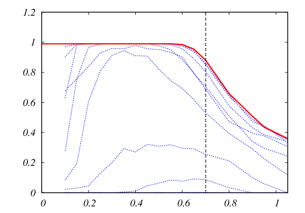
aRefer to caption Refer to caption λ 0 θ θ Psucc

Figure 2: Learning random subgraphs of a 7×77\times 7 (p=49p=49) two-dimensional grid from n=4500n=4500 Ising models samples, using regularized logistic regression. Left: success probability as a function of the model parameter θ\theta and of the regularization parameter λ0\lambda_{0} (darker corresponds to highest probability). Right: the same data plotted for several choices of λ\lambda versus θ\theta. The vertical line corresponds to the model critical temperature. The thick line is an envelope of the curves obtained for different λ\lambda, and should correspond to optimal regularization.

Figure reports the success probability of 𝖱𝗅𝗋⁡(λ){\sf Rlr}(\lambda) when applied to random subgraphs of a 7×77\times 7 two-dimensional grid. Each such graphs was obtained by removing each edge independently with probability ρ=0.3\rho=0.3. Success probability was estimated by applying 𝖱𝗅𝗋⁡(λ){\sf Rlr}(\lambda) to each vertex of 88 graphs (thus averaging over 392392 runs of 𝖱𝗅𝗋⁡(λ){\sf Rlr}(\lambda)), using n=4500n=4500 samples. We scaled the regularization parameter as λ=2​λ0​θ​(log⁡p/n)1/2\lambda=2\lambda_{0}\theta(\log p/n)^{1/2} (this choice is motivated by the algorithm analysis [11] and is empirically the most satisfactory), and searched over λ0\lambda_{0}.

The data clearly illustrate the phenomenon discussed in the previous pages. Despite the large number of samples n≫log⁡pn\gg\log p, when θ\theta crosses a threshold, the algorithm starts performing poorly irrespective of λ\lambda. Intriguingly, this threshold is not far from the critical point of the Ising model on a randomly diluted grid θcrit​(ρ=0.3)≈0.7\theta_{\rm crit}(\rho=0.3)\approx 0.7 [34, 35].

aRefer to caption Refer to caption Psucc = θ 0.10 = θ 0.15 = θ 0.45 = θ 0.45 n θ Psucc

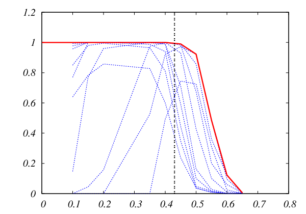
Figure 3: Learning uniformly random graphs of degree Δ=4\Delta=4 from Ising models samples, using regularized logistic regression. Left: success probability as a function of the number of samples nn for several values of θ\theta. Dotted: θ=0.10\theta=0.10, 0.150.15, 0.200.20, 0.350.35, 0.400.40 (in all these cases θ<θthr​(Δ=4)\theta<\theta_{\rm thr}(\Delta=4)). Dashed: θ=0.45\theta=0.45, 0.500.50, 0.550.55, 0.600.60, 0.650.65 (θ>θthr​(4)\theta>\theta_{\rm thr}(4), some of these are indistinguishable from the axis). Right: the same data plotted for several choices of λ\lambda versus θ\theta as in Fig. 2, right panel.

Figure 3 presents similar data when GG is a uniformly random graph of degree Δ=4\Delta=4, over p=50p=50 vertices. The evolution of the success probability with nn clearly shows a dichotomy. When θ\theta is below a threshold, a small number of samples is sufficient to reconstruct GG with high probability. Above the threshold even n=104n=10^{4} samples are to few. In this case we can predict the threshold analytically, cf. Lemma 33 below, and get θthr​(Δ=4)≈0.4203\theta_{\rm thr}(\Delta=4)\approx 0.4203, which compares favorably with the data.

4 Proofs

4.1 Notation and important remarks

Before proceeding it is convenient to introduce some notation and make some important remarks. If VV is a matrix and RR is an index set then VRV_{R} denotes the vector formed by all entries whose index lies in RR and similarly, if MM is a matrix and R,PR,P are index sets then MR​PM_{R\;P} denotes the submatrix with row indices in RR and column indices in PP. As before, we let rr be the vertex whose neighborhood we are trying to reconstruct and define S=∂rS={\partial r} and Sc=V∖∂r∪rS^{c}=V\setminus{{\partial r}\cup r}. Since the cost function L⁡(θ¯,{x¯(ℓ)})+λ​‖θ¯‖1L(\underline{\theta};\{\underline{x}^{(\ell)}\})+\lambda\|\underline{\theta}\|_{1} only depends on θ¯\underline{\theta} through its components θ¯r,⋅={θr​j}\underline{\theta}_{r,\cdot}=\{\theta_{rj}\}, we will hereafter neglect all the other parameters and write θ¯\underline{\theta} as a shorthand of θ¯r,⋅\underline{\theta}_{r,\cdot}.

Let z^∗\hat{z}^{*} be a subgradient of ‖θ¯‖1\|\underline{\theta}\|_{1} evaluated at the true parameters values, θ¯∗={θr​j:θi​j=0,∀j∉∂r,θr​j=θ,∀j∈∂r}\underline{\theta}^{*}=\{\theta_{rj}:\theta_{ij}=0,\;\forall j\notin{\partial r},\theta_{rj}=\theta,\;\forall j\in{\partial r}\}. Let θ¯^n\hat{\underline{\theta}}^{n} be the parameter estimate returned by 𝖱𝗅𝗋⁡(λ){\sf Rlr}(\lambda) when the number of samples is nn. Note that, since we assumed θ¯∗≥0\underline{\theta}^{*}\geq 0, we have θ¯S∗>0\underline{\theta}_{S}^{*}>0 and hence z^S∗=𝟙\hat{z}^{*}_{S}=\mathbbm{1}. Define Qn​(θ¯,{x¯(ℓ)})Q^{n}(\underline{\theta};\{\underline{x}^{(\ell)}\}) to be the Hessian of L⁡(θ¯,{x(ℓ)})L(\underline{\theta};\{x^{(\ell)}\}) and Q⁡(θ¯)=limn→∞Qn​(θ¯,{x¯(ℓ)})Q(\underline{\theta})=\lim_{n\rightarrow\infty}Q^{n}(\underline{\theta};\{\underline{x}^{(\ell)}\}). By the law of large numbers Q⁡(θ¯)Q(\underline{\theta}) exists a.s. and is the Hessian of 𝔼G,θ¯​log⁡ℙG,θ¯​(Xr|X\r){\mathbb{E}}_{G,\underline{\theta}}\log{\mathbb{P}}_{G,\underline{\theta}}(X_{r}|X_{\backslash r}) where 𝔼G,θ¯{\mathbb{E}}_{G,\underline{\theta}} is the expectation with respect to (19) and X¯\underline{X} is a random variable distributed according to (19). It is convenient to recall here the expressions for the Hessian and gradient of LL for finite nn and in the limit when n→∞n\rightarrow\infty. For all i,j∈V\{r}i,j\in V\backslash\{r\} we have,

Qi​jn​(θ¯)\displaystyle Q^{n}_{ij}(\underline{\theta}) =1n​∑ℓ=1nxi(ℓ)​xj(ℓ)cosh2⁡(∑t∈V\{r}θr​t​xt(ℓ)),\displaystyle=\frac{1}{n}\sum^{n}_{\ell=1}\frac{x^{(\ell)}_{i}x^{(\ell)}_{j}}{\cosh^{2}\left(\sum_{t\in V\backslash\{r\}}\theta_{rt}x^{(\ell)}_{t}\right)}, (21)
Qi​j​(θ¯)\displaystyle Q_{ij}(\underline{\theta}) =𝔼G,θ¯∗​(Xi​Xjcosh2⁡(∑t∈V\{r}θr​t​Xt)),\displaystyle={\mathbb{E}}_{G,\underline{\theta}^{*}}\left(\frac{X_{i}X_{j}}{\cosh^{2}(\sum_{t\in V\backslash\{r\}}\theta_{rt}X_{t})}\right), (22)
[∇Ln​(θ¯)]i\displaystyle[\nabla L^{n}(\underline{\theta})]_{i} =1n​∑ℓ=1nxi(ℓ)​(tanh⁡(∑t∈V\{r}θr​t​xt(ℓ))−xr(ℓ)),\displaystyle=\frac{1}{n}\sum^{n}_{\ell=1}x^{(\ell)}_{i}\Big(\tanh\Big(\sum_{t\in V\backslash\{r\}}\theta_{rt}x^{(\ell)}_{t}\Big)-x^{(\ell)}_{r}\Big), (23)
[∇L​(θ¯)]i\displaystyle[\nabla L(\underline{\theta})]_{i} =𝔼G,θ¯∗​{Xi​tanh⁡(∑t∈V\{r}θr​t​Xt)}−𝔼G,θ¯∗​{Xi​Xr}.\displaystyle={\mathbb{E}}_{G,\underline{\theta}^{*}}\Big\{X_{i}\tanh\Big(\sum_{t\in V\backslash\{r\}}\theta_{rt}X_{t}\Big)\Big\}-{\mathbb{E}}_{G,\underline{\theta}^{*}}\{X_{i}X_{r}\}. (24)

Note that from the last expression it follows that ∇L​(θ¯∗)=0\nabla L(\underline{\theta}^{*})=0.

We will denote the maximum and minimum eigenvalue of a symmetric matrix MM by σmax​(M)\sigma_{\rm max}(M) and σmin​(M)\sigma_{\rm min}(M) respectively. Recall that ‖M‖∞=max⁡∑ji⁡|Mi​j|\|M\|_{\infty}=\max_{i}\sum_{j}|M_{ij}|.

We will omit arguments whenever clear from the context. Any quantity evaluated at the true parameter values will be represented with a ∗, e.g. Q∗=Q⁡(θ∗)Q^{*}=Q(\theta^{*}). Quantities under a ∧\wedge depend on nn. When clear from the context and since all the examples that we work on have θi​j∈{0,θ\theta_{ij}\in\{0,\theta }, we will write 𝔼G,θ{\mathbb{E}}_{G,\theta} as 𝔼G,θ¯{\mathbb{E}}_{G,\underline{\theta}} or even simply 𝔼{\mathbb{E}}. Similarly, ℙG,θ¯{\mathbb{P}}_{G,\underline{\theta}} will be sometimes written as simply ℙG,θ{\mathbb{P}}_{G,\theta} or just ℙ{\mathbb{P}}. A subscript nn under ℙG,θ¯{\mathbb{P}}_{G,\underline{\theta}}, i.e. ℙn,G,θ¯{\mathbb{P}}_{n,G,\underline{\theta}}, will be introduced to denote the product measure formed by nn copies of model (19). Through out this section Psucc{\rm P}_{\rm succ} will denote the probability of success of a given algorithm, that is, the probability that the algorithm is able to recover the underlying GG exactly.

Throughout this section GG is a graph of maximum degree Δ\Delta.

4.2 Simple Thresholding

In the following we let Ci​j≡𝔼G,θ​{Xi​Xj}C_{ij}\equiv{\mathbb{E}}_{G,\theta}\{X_{i}X_{j}\} where expectation is taken with respect to the Ising model (1).

Proof.

(Theorem 2.1 ) If GG is a tree then Ci​j=tanh⁡θC_{ij}=\tanh\theta for all (i​j)∈E(ij)\in E and Ci​j≤tanh2⁡θC_{ij}\leq\tanh^{2}\theta for all (i​j)∉E(ij)\notin E. To see this notice that only paths that connect ii to jj contribute to Ci​jC_{ij} and given that GG is a tree there is only one such path and its length is exactly 1 if (i,j)∈E(i,j)\in E and at least 2 when (i,j)∉E(i,j)\notin E. The probability that 𝖳𝗁𝗋⁡(τ){\sf Thr}(\tau) fails is

1−Psucc=ℙn,G,θ{C^i​j<τ for some (i,j)∈EorC^i​j≥τ for some (i,j)∉E}.\displaystyle 1-{\rm P}_{\rm succ}={\mathbb{P}}_{n,G,\theta}\{\widehat{C}_{ij}<\tau\mbox{ for some }(i,j)\in E\;{\rm or}\;\widehat{C}_{ij}\geq\tau\;\mbox{ for some }\;(i,j)\notin E\}\,. (25)

Let τ=(tanh⁡θ+tanh2⁡θ)/2\tau=(\tanh\theta+\tanh^{2}\theta)/2. Applying Azuma-Hoeffding inequality to C^i​j=1n​∑ℓ=1nxi(ℓ)​xj(ℓ)\widehat{C}_{ij}=\frac{1}{n}\sum^{n}_{\ell=1}x^{(\ell)}_{i}x^{(\ell)}_{j} we have that if (i,j)∈E(i,j)\in E then,

ℙn,G,θ​(C^i​j<τ)=ℙn,G,θ​(∑ℓ=1n(xi(ℓ)​xj(ℓ)−Ci​j)<n⁡(τ−tanh⁡θ))≤e−132​n​(tanh⁡θ−tanh2⁡θ)2{\mathbb{P}}_{n,G,\theta}(\widehat{C}_{ij}<\tau)={\mathbb{P}}_{n,G,\theta}\left(\sum^{n}_{\ell=1}(x^{(\ell)}_{i}x^{(\ell)}_{j}-C_{ij})<n(\tau-\tanh\theta)\right)\leq e^{-\frac{1}{32}n(\tanh\theta-\tanh^{2}\theta)^{2}} (26)

and if (i,j)∉E(i,j)\notin E then similarly,

ℙn,G,θ​(C^i​j≥τ)=ℙn,G,θ​(∑ℓ=1n(xi(ℓ)​xj(ℓ)−Ci​j)≥n⁡(τ−tanh2⁡θ))≤e−132​n​(tanh⁡θ−tanh2⁡θ)2.{\mathbb{P}}_{n,G,\theta}(\widehat{C}_{ij}\geq\tau)={\mathbb{P}}_{n,G,\theta}\left(\sum^{n}_{\ell=1}(x^{(\ell)}_{i}x^{(\ell)}_{j}-C_{ij})\geq n(\tau-\tanh^{2}\theta)\right)\leq e^{-\frac{1}{32}n(\tanh\theta-\tanh^{2}\theta)^{2}}. (27)

Applying union bound over the two possibilities, (i,j)∈E(i,j)\in E or (i,j)∉E(i,j)\notin E, and over the edges (|E|<p2/2|E|<p^{2}/2), we can bound Psucc{\rm P}_{\rm succ} by

Psucc≥1−p2​e−132​n​(tanh⁡θ−tanh2⁡θ)2.\displaystyle{\rm P}_{\rm succ}\geq 1-p^{2}\,e^{-\frac{1}{32}n(\tanh\theta-\tanh^{2}\theta)^{2}}\,. (28)

Imposing the right hand side to be larger than δ\delta proves our result. ∎

Proof.

(Theorem 2.2) We will prove that, for θ<arctanh⁡(1/(2​Δ))\theta<{\rm arctanh}(1/(2\Delta)), Ci​j≥tanh⁡θC_{ij}\geq\tanh\theta for all (i,j)∈E(i,j)\in E and Ci​j≤1/(2​Δ)C_{ij}\leq 1/(2\Delta) for all (i​j)∉E(ij)\notin E. In particular Ci​j<Ck​lC_{ij}<C_{kl} for all (i,j)∉E(i,j)\notin E and all (k,l)∈E(k,l)\in E . The theorem follows from this fact via union bound and Azuma-Hoeffding inequality as in the proof of Theorem 2.1.

The bound Ci​j≥tanh⁡θC_{ij}\geq\tanh\theta for (i​j)∈E(ij)\in E is a direct consequence of Griffiths inequality [36] : compare the expectation of xi​xjx_{i}x_{j} in GG with the same expectation in the graph that only includes edge (i,j)(i,j).

The second bound is derived using the technique of [35], i.e., bound Ci​jC_{ij} by the generating function for self-avoiding walks on the graphs from ii to jj. More precisely, assume l=dist⁡(i,j)l={\rm dist}(i,j) and denote by Ni​j​(k)N_{ij}(k) the number of self avoiding walks of length kk between ii and jj on GG. Then [35] proves that

Ci​j≤∑k=l∞(tanh⁡θ)k​Ni​j​(k)≤∑n=l∞Δk−1​(tanh⁡θ)k≤Δl−1​(tanh⁡θ)l1−Δ​tanh⁡θ≤Δ​(tanh⁡θ)21−Δ​tanh⁡θ.\displaystyle C_{ij}\leq\sum^{\infty}_{k=l}(\tanh\theta)^{k}N_{ij}(k)\leq\sum^{\infty}_{n=l}\Delta^{k-1}(\tanh\theta)^{k}\leq\frac{\Delta^{l-1}(\tanh\theta)^{l}}{1-\Delta\tanh\theta}\leq\frac{\Delta(\tanh\theta)^{2}}{1-\Delta\tanh\theta}. (29)

If θ<arctanh⁡(1/(2​Δ))\theta<{\rm arctanh}(1/(2\Delta)) the above implies Ci​j≤1/(2​Δ)C_{ij}\leq 1/(2\Delta) which is our claim. ∎

Proof.

(Theorem 2.3) The theorem is proved by constructing GG as follows: sample a uniformly random regular graph of degree Δ\Delta over the p−2p-2 vertices {1,2,…,p−2}≡[p−2]\{1,2,\dots,p-2\}\equiv[p-2]. Add an extra edge between nodes p−1p-1 and pp. The resulting graph is not connected. We claim that for θ>K/Δ\theta>K/\Delta and with probability converging to 11 as p→∞p\to\infty, there exist i,j∈[p−2]i,j\in[p-2] such that (i,j)∉E(i,j)\notin E and Ci​j>Cp−1,pC_{ij}>C_{p-1,p}. As a consequence, thresholding fails.

Obviously Cp−1,p=tanh⁡θC_{p-1,p}=\tanh\theta. Choose i∈[p−2]i\in[p-2] uniformly at random, and jj a node at a fixed distance tt from ii. We can compute Ci​jC_{ij} as p→∞p\to\infty using the same local weak convergence result as in the proof of Lemma 33. Namely, Ci​jC_{ij} converges to the correlation between the root and a leaf node in the tree Ising model (45). In particular one can show, [33], that

limp→∞Ci​j≥m​(θ)2,\displaystyle\lim_{p\to\infty}C_{ij}\geq m(\theta)^{2}\,, (30)

where m⁡(θ)=tanh⁡(Δ​h∗/(Δ−1))m(\theta)=\tanh(\Delta h^{*}/(\Delta-1)) and h∗h^{*} is the unique positive solution of Eq. (46).

The proof is completed by showing that tanh⁡θ<m​(θ)2\tanh\theta<m(\theta)^{2} for all θ>K/Δ\theta>K/\Delta. ∎

4.3 Proof of Theorem 2.8: failure of regularized logistic regression

In order to prove Theorem 2.8, we need a few auxiliary results. Our first auxiliary results establishes that, if λ\lambda is small, then ‖QSc​S∗​QS​S∗−1​z^S∗‖∞>1\|Q^{*}_{S^{c}S}{Q^{*}_{SS}}^{-1}\hat{z}^{*}_{S}\|_{\infty}>1 is a sufficient condition for the failure of 𝖱𝗅𝗋⁡(λ){\sf Rlr}(\lambda). We recall here that the subgradient of ‖θ¯‖1\|\underline{\theta}\|_{1} evaluated at θ¯∗\underline{\theta}^{*},that is z^∗\hat{z}^{*}, satisfies z^S∗=𝟙\hat{z}^{*}_{S}={\mathbbm{1}}.

Lemma 4.1.

Assume [QSc​S∗​QS​S∗−1​z^S∗]i≥1+ϵ[Q^{*}_{S^{c}S}{Q^{*}_{SS}}^{-1}\hat{z}^{*}_{S}]_{i}\geq 1+\epsilon for some ϵ>0\epsilon>0 and some row i∈Vi\in V, σmin​(QS​S∗)≥Cmin>0\sigma_{\rm min}(Q^{*}_{SS})\geq C_{\rm min}>0, and λ<Cmin3​ϵ/(27​(1+ϵ2)​Δ3)\lambda<C^{3}_{\min}\epsilon/(2^{7}(1+\epsilon^{2})\Delta^{3}). Then the success probability of 𝖱𝗅𝗋⁡(λ){\sf Rlr}(\lambda) is upper bounded as

Psucc≤4​Δ2​e−n​δA2+4​Δ​e−n​λ2​δB2{\rm P}_{\rm succ}\leq 4\Delta^{2}e^{-n\delta_{A}^{2}}+4\Delta\,e^{-n\lambda^{2}\delta_{B}^{2}} (31)

where δA=(Cmin2/32​Δ)​ϵ\delta_{A}=(C_{\rm min}^{2}/32\Delta)\epsilon and δB=(Cmin/64​Δ)​ϵ\delta_{B}=(C_{\rm min}/64\sqrt{\Delta})\epsilon.

The next Lemma implies that, for λ\lambda to be ‘reasonable’ (in the sense introduced in Section 2.2.2), n​λ2n\lambda^{2} must be unbounded with respect to pp. In fact, by this lemma, if we choose nn to be very large and choose a sequence of star graphs of increasing number of nodes but with only one edge between the central node and the remaining nodes, then, unless KK is increasing with pp, 𝖱𝗅𝗋⁡(λ){\sf Rlr}(\lambda) will fail to reconstruct the graph with a probability greater than 1/21/2, which is a contradiction if λ\lambda is ‘reasonable’.

Lemma 4.2.

There exist M=M⁡(K,θ)>0M=M(K,\theta)>0 decreasing with KK for θ>0\theta>0 such that the following is true: If GG is the (star) graph with vertex set V=[p]V=[p] and edge set E={(r,i)}E=\{(r,i)\} (e.g. r=1r=1, i=2i=2) and n​λ2≤Kn\lambda^{2}\leq K, then

Psucc≤e−M⁡(K,θ)​p+e−n(1−tanhθ)2/32.{\rm P}_{\rm succ}\leq e^{-M(K,\theta)p}+e^{-n(1-\tanh\theta)^{2}/32}\,. (32)

Finally, our key result shows that the condition ‖QSc​S∗​QS​S∗−1​z^S∗‖∞≤1\|Q^{*}_{S^{c}S}{Q^{*}_{SS}}^{-1}\hat{z}^{*}_{S}\|_{\infty}\leq 1 is violated with high probability for large random graphs. The proof of this result relies on a local weak convergence result for ferromagnetic Ising models on random graphs proved in [32].

Lemma 4.3.

Let GG be a uniformly random regular graph of degree Δ>3\Delta>3. Then, there exists θthr​(Δ)\theta_{\rm thr}(\Delta) such that, for θ>θthr​(Δ)\theta>\theta_{\rm thr}(\Delta), ‖QSc​S∗​QS​S∗−1​z^S∗‖∞≥1+ϵ⁡(θ,Δ)\|Q^{*}_{S^{c}S}{Q^{*}_{SS}}^{-1}\hat{z}^{*}_{S}\|_{\infty}\geq 1+\epsilon(\theta,\Delta) with probability converging to 11 as p→∞p\to\infty (ϵ⁡(θ,Δ)>0\epsilon(\theta,\Delta)>0 and ϵ⁡(θ,Δ)→0\epsilon(\theta,\Delta)\rightarrow 0 as θ→∞\theta\rightarrow\infty).

Furthermore, for large Δ\Delta, θthr​(Δ)=θ~​Δ−1​(1+o⁡(1))\theta_{\rm thr}(\Delta)=\tilde{\theta}\,\Delta^{-1}(1+o(1)). The constant θ~\tilde{\theta} is given by θ~=h∞2\tilde{\theta}=h^{2}_{\infty} and h∞h_{\infty} is the unique positive solution of

h∞tanhh∞=1.h_{\infty}\tanh h_{\infty}=1. (33)

Finally, there exist Cmin>0C_{\rm min}>0 dependent only on Δ\Delta and θ\theta such that σmin​(QS​S∗)≥Cmin\sigma_{\rm min}(Q^{*}_{SS})\geq C_{\rm min} with probability converging to 11 as p→∞p\to\infty.

The proofs of Lemmas 4.1, 32 and 33 are sketched in the next subsection.

Proof.

(Theorem 2.8) Fix Δ>3\Delta>3, θ>K/Δ\theta>K/\Delta (where KK is a large enough constant independent of Δ\Delta), and ϵ,Cmin>0\epsilon,C_{\rm min}>0 and both small enough. By Lemma 33, for any pp large enough we can choose a Δ\Delta-regular graph Gp=(V=[p],Ep)G_{p}=(V=[p],E_{p}) and vertex r∈Vr\in V such that |QSc​S∗​QS​S∗−1​z^S∗|i>1+ϵ|Q^{*}_{S^{c}S}{Q^{*}_{SS}}^{-1}\hat{z}^{*}_{S}|_{i}>1+\epsilon for some i∈V∖ri\in V\setminus r (Indeed most vertices rr and graphs GpG_{p} will work).

By Theorem 1 in [10] we can assume without loss of generality n>K′​Δ​log⁡pn>K^{\prime}\Delta\log p for some small constant K′K^{\prime}. Further by Lemma 32, n​λ2≥F⁡(p)n\lambda^{2}\geq F(p) for some F⁡(p)↑∞F(p)\uparrow\infty as p→∞p\to\infty and the condition of Lemma 4.1 on λ\lambda is satisfied since by the assumption that λ\lambda is ‘reasonable’ we have λ→0\lambda\to 0 as n→∞n\rightarrow\infty. Using these results in Eq. (31) of Lemma 4.1 we get the following upper bound on the success probability

Psucc​(Gp)≤4​Δ2​p−δA2​K′​Δ+2​Δ​e−F⁡(p)​δB2.{\rm P}_{\rm succ}(G_{p})\leq 4\Delta^{2}p^{-\delta_{A}^{2}K^{\prime}\Delta}+2\Delta\,e^{-F(p)\delta_{B}^{2}}\,. (34)

In particular Psucc​(Gp)→0{\rm P}_{\rm succ}(G_{p})\to 0 as p→∞p\to\infty. ∎

4.3.1 Proofs of auxiliary lemmas

Proof.

(Lemma 4.1) This proof follows closely the proof of Proposition 1 in [11]. For a matter of clarify of exposition we will include all the steps, even if these do not differ from the exposition done in [11].

We will show that (under the assumptions of the Lemma on the Incoherence Condition, σmin​(QS​S∗)\sigma_{\min}(Q^{*}_{SS}) and λ\lambda) if θ¯^=(θ¯^S,θ¯^SC)=(θ¯^S,0)\hat{\underline{\theta}}=(\hat{\underline{\theta}}_{S},\hat{\underline{\theta}}_{S^{C}})=(\hat{\underline{\theta}}_{S},0) with θ¯^S>0\hat{\underline{\theta}}_{S}>0 then the probability that 𝖱𝗅𝗋⁡(λ){\sf Rlr}(\lambda) returns θ¯^\hat{\underline{\theta}} is upper bounded as in Eq. (31). More specifically, we will show that this θ¯^\hat{\underline{\theta}} will not satisfy the stationarity condition ∇L​(θ¯^)+λ​z^=0\nabla L(\hat{\underline{\theta}})+\lambda\hat{z}=0 with high probability for any subgradient z^\hat{z} of the function ‖θ¯‖1\|\underline{\theta}\|_{1} at θ¯^\hat{\underline{\theta}}.

To simplify notation we will omit {x¯(ℓ)}\{\underline{x}^{(\ell)}\} in all the expressions involving and derived from LL.

Assume the event ∇L​(θ¯^)+λ​z^=0\nabla L(\hat{\underline{\theta}})+\lambda\hat{z}=0 holds for some θ¯^\hat{\underline{\theta}} as specified above. An application of the mean value theorem yields

∇2L​(θ¯∗)​[θ¯^−θ¯∗]=Wn−λ​z^−Rn,\nabla^{2}L(\underline{\theta}^{*})[\hat{\underline{\theta}}-\underline{\theta}^{*}]=W^{n}-\lambda\hat{z}-R^{n}\,, (35)

where Wn=−∇L​(θ¯∗)W^{n}=-\nabla L(\underline{\theta}^{*}) and [Rn]j=[∇2L​(θ¯¯(j))−∇2L​(θ¯∗)]jT​(θ¯^−θ¯∗)[R^{n}]_{j}=[\nabla^{2}L(\bar{\underline{\theta}}^{(j)})-\nabla^{2}L(\underline{\theta}^{*})]_{j}^{T}(\hat{\underline{\theta}}-\underline{\theta}^{*}) with θ¯¯(j)\bar{\underline{\theta}}^{(j)} a point in the line from θ¯^\hat{\underline{\theta}} to θ¯∗\underline{\theta}^{*}. Notice that by definition ∇2L​(θ¯∗)=Qn∗=Qn​(θ¯∗)\nabla^{2}L(\underline{\theta}^{*})={Q^{n}}^{*}=Q^{n}(\underline{\theta}^{*}). To simplify notation we will omit the ∗* in all Qn∗{Q^{n}}^{*}. All QnQ^{n} in this proof are thus evaluated at θ¯∗\underline{\theta}^{*}.

Breaking this expression into its SS and SCS^{C} components and since θ¯^SC=θ¯SC∗=0\hat{\underline{\theta}}_{S^{C}}=\underline{\theta}^{*}_{S^{C}}=0 we can write

QSC​Sn​(θ¯^S−θ¯S∗)\displaystyle Q^{n}_{S^{C}S}(\hat{\underline{\theta}}_{S}-\underline{\theta}_{S}^{*}) =WSCn−λ​z^SC+RSCn,\displaystyle=W^{n}_{S^{C}}-\lambda\hat{z}_{S^{C}}+R_{S^{C}}^{n}, (36)
QS​Sn​(θ¯^S−θ¯S∗)\displaystyle Q^{n}_{SS}(\hat{\underline{\theta}}_{S}-\underline{\theta}_{S}^{*}) =WSn−λ​z^S+RSn.\displaystyle=W^{n}_{S}-\lambda\hat{z}_{S}+R_{S}^{n}. (37)

Eliminating θ¯^S−θ¯S∗\hat{\underline{\theta}}_{S}-\underline{\theta}_{S}^{*} from the two expressions we obtain

[WSCn−RSCn]−QSC​Sn​(QS​Sn)−1​[WSn−RSn]+λ​QSC​Sn​(QS​Sn)−1​z^S=λ​z^SC.[W^{n}_{S^{C}}-R^{n}_{S^{C}}]-Q^{n}_{S^{C}S}(Q^{n}_{SS})^{-1}[W^{n}_{S}-R^{n}_{S}]+\lambda Q^{n}_{S^{C}S}(Q^{n}_{SS})^{-1}\hat{z}_{S}=\lambda\hat{z}_{S^{C}}\,. (38)

Now notice that QSC​Sn​(QS​Sn)−1=T1+T2+T3+T4Q^{n}_{S^{C}S}(Q^{n}_{SS})^{-1}=T_{1}+T_{2}+T_{3}+T_{4} where

T1\displaystyle T_{1} =QSC​S∗​[(QS​Sn)−1−(QS​S∗)−1],T2=[QSC​Sn−QSC​S∗]​QS​S∗−1,\displaystyle=Q^{*}_{S^{C}S}[(Q^{n}_{SS})^{-1}-(Q^{*}_{SS})^{-1}]\,,\;\;\;\;\;\;\;\;\;\;\;\;\;\;\;\;\;\;\;\;\;\;\;\;\;T_{2}=[Q^{n}_{S^{C}S}-Q^{*}_{S^{C}S}]{Q^{*}_{SS}}^{-1}\,,
T3\displaystyle T_{3} =[QSC​Sn−QSC​S∗]​[(QS​Sn)−1−(QS​S∗)−1],T4=QSC​S∗​QS​S∗−1.\displaystyle=[Q^{n}_{S^{C}S}-Q^{*}_{S^{C}S}][(Q^{n}_{SS})^{-1}-(Q^{*}_{SS})^{-1}]\,,\;\;\;\;\;\;\;\;\;\;T_{4}=Q^{*}_{S^{C}S}{Q^{*}_{SS}}^{-1}\,.

Recalling that z^S=𝟙\hat{z}_{S}={\mathbbm{1}} and using the above decomposition we can lower bound the absolute value of the indexed-ii component of z^SC\hat{z}_{S^{C}} by

|z^i|≥‖[QSC​S∗​QS​S∗−1​z^S]i‖∞−‖T1,i‖1−‖T2,i‖1−‖T3,i‖1\displaystyle|\hat{z}_{i}|\geq\|[Q^{*}_{S^{C}S}{Q^{*}_{SS}}^{-1}\hat{z}_{S}]_{i}\|_{\infty}-\|T_{1,i}\|_{1}-\|T_{2,i}\|_{1}-\|T_{3,i}\|_{1} (39)
−|Winλ|−|Rinλ|−|[QSC​Sn​(QS​Sn)−1]i|(‖WSnλ‖∞+‖RSnλ‖∞).\displaystyle-\Big|\frac{W^{n}_{i}}{\lambda}\Big|-\Big|\frac{R^{n}_{i}}{\lambda}\Big|-\|[Q^{n}_{S^{C}S}(Q^{n}_{SS})^{-1}]_{i}\|\left(\Big\|\frac{W^{n}_{S}}{\lambda}\Big\|_{\infty}+\Big\|\frac{R^{n}_{S}}{\lambda}\Big\|_{\infty}\right).

We will now assume that the samples {x(ℓ)}\{x^{(\ell)}\} are such that the following event holds (notice that i∈SCi\in S^{C}),

ℰi≡{‖QS∪{i}​Sn−QS∪{i}​S∗‖∞<ξA,‖WS∪{i}nλ‖∞<ξB},{\cal E}_{i}\equiv\Big\{\|Q^{n}_{S\cup\{i\}\;S}-Q^{*}_{S\cup\{i\}\;S}\|_{\infty}<\xi_{A},\Big\|\frac{W^{n}_{S\cup\{i\}}}{\lambda}\Big\|_{\infty}<\xi_{B}\Big\}\,, (40)

where ξA≡Cmin2​ϵ/(8​Δ)\xi_{A}\equiv C_{\rm min}^{2}\epsilon/(8\Delta) and ξB≡Cmin​ϵ/(16​Δ)\xi_{B}\equiv C_{\rm min}\epsilon/(16\sqrt{\Delta}).

From relations (21) to (24) in Section 4.1 we know that 𝔼G,θ​(Qn)=Q∗\mathbb{E}_{G,\theta}(Q^{n})=Q^{*}, 𝔼G,θ​(Wn)=0{\mathbb{E}}_{G,\theta}(W^{n})=0 and that both Qn−Q∗Q^{n}-Q^{*} and WnW^{n} are sums i.i.d. random variables bounded by 2. From this, a simple application of Azuma-Hoeffding inequality yields 44 4 For full details see the proof of Lemma 2 and the discussion following Lemma 6 in [11].

ℙn,G,θ​(|Qi​jn−Qi​j∗|>δ)≤2​e−δ2​n8,\displaystyle{\mathbb{P}}_{n,G,\theta}(|Q_{ij}^{n}-Q_{ij}^{*}|>\delta)\leq 2e^{-\frac{\delta^{2}n}{8}}, (41)
ℙn,G,θ​(|Wi​jn|>δ)≤2​e−δ2​n8,\displaystyle{\mathbb{P}}_{n,G,\theta}(|W_{ij}^{n}|>\delta)\leq 2e^{-\frac{\delta^{2}n}{8}}, (42)

for all ii and jj. Applying union bound we conclude that the event ℰi{\cal E}_{i} holds with probability at least

1−2​Δ​(Δ+1)​e−n​ξA28−2​(Δ+1)​e−n​λ2​ξB28≥1−4​Δ2​e−n​δA2−4​Δ​e−n​λ2​δB,\displaystyle 1-2\Delta(\Delta+1)e^{-\frac{n\xi^{2}_{A}}{8}}-2(\Delta+1)e^{-\frac{n\lambda^{2}\xi^{2}_{B}}{8}}\geq 1-4\Delta^{2}e^{-n\delta^{2}_{A}}-4\Delta e^{-n\lambda^{2}\delta_{B}}, (43)

where δA=Cmin2​ϵ/(32​Δ)\delta_{A}=C^{2}_{\min}\epsilon/(32\Delta) and δB=Cmin​ϵ/(64​Δ)\delta_{B}=C_{\min}\epsilon/(64\sqrt{\Delta}).

If the event ℰi{\cal E}_{i} holds then σmin​(QS​Sn)>σmin​(QS​S∗)−Cmin/2>Cmin/2\sigma_{\rm min}(Q^{n}_{SS})>\sigma_{\rm min}(Q^{*}_{SS})-C_{\rm min}/2>C_{\rm min}/2. Since ‖[QSC​Sn​(QS​Sn)−1]i‖∞≤‖QS​Sn−1‖2​‖QS​in‖2\|[Q^{n}_{S^{C}S}(Q^{n}_{SS})^{-1}]_{i}\|_{\infty}\leq\|{Q^{n}_{SS}}^{-1}\|_{2}\|Q^{n}_{Si}\|_{2} and |Qj​in|≤1​∀i,j|Q^{n}_{ji}|\leq 1\forall i,j we can write ‖[QSC​Sn​(QS​Sn)−1]i‖∞≤2​Δ/Cmin\|[Q^{n}_{S^{C}S}(Q^{n}_{SS})^{-1}]_{i}\|_{\infty}\leq 2\sqrt{\Delta}/C_{\min} and simplify our lower bound to

|z^i|≥‖[QSC​S∗​QS​S∗−1​z^S]i‖∞−‖T1,i‖1−‖T2,i‖1−‖T3,i‖1\displaystyle|\hat{z}_{i}|\geq\|[Q^{*}_{S^{C}S}{Q^{*}_{SS}}^{-1}\hat{z}_{S}]_{i}\|_{\infty}-\|T_{1,i}\|_{1}-\|T_{2,i}\|_{1}-\|T_{3,i}\|_{1} (44)
−|Winλ|−|Rinλ|−2​ΔCmin​(‖WSnλ‖∞+‖RSnλ‖∞).\displaystyle-\Big|\frac{W^{n}_{i}}{\lambda}\Big|-\Big|\frac{R^{n}_{i}}{\lambda}\Big|-\frac{2\sqrt{\Delta}}{C_{\min}}\left(\Big\|\frac{W^{n}_{S}}{\lambda}\Big\|_{\infty}+\Big\|\frac{R^{n}_{S}}{\lambda}\Big\|_{\infty}\right).

The proof is completed by showing that the event ℰi{\cal E}_{i} and the assumptions of the theorem imply that each of last 77 terms in this expression is smaller than ϵ/8\epsilon/8. Since |[QSC​S∗​QS​S∗−1]iT​z^Sn|≥1+ϵ|[Q^{*}_{S^{C}S}{Q^{*}_{SS}}^{-1}]_{i}^{T}\hat{z}^{n}_{S}|\geq 1+\epsilon by assumption, this implies |z^i|≥1+ϵ/8>1|\hat{z}_{i}|\geq 1+\epsilon/8>1 which cannot be true since any subgradient of the 11-norm has components of magnitude at most 11.

Taking into account that σmin​(QS​S∗)≤maxi​j⁡Qi​j∗≤1\sigma_{\min}(Q^{*}_{SS})\leq\max_{ij}Q^{*}_{ij}\leq 1 and that Δ>1\Delta>1, the last condition on ℰi{\cal E}_{i} immediately bounds all terms involving WnW^{n} by ϵ/8\epsilon/8. Some straightforward manipulations imply (see Lemma 7 from [11] for a similar computation)

‖T1,i‖1\displaystyle\|T_{1,i}\|_{1} ≤ΔCmin2​‖QS​Sn−QS​S∗‖∞,‖T2,i‖1≤ΔCmin​‖[QSC​Sn−QSC​S∗]i‖∞,\displaystyle\leq\frac{\Delta}{C_{\rm min}^{2}}\|Q^{n}_{SS}-Q^{*}_{SS}\|_{\infty}\,,\;\;\;\;\;\;\;\;\;\|T_{2,i}\|_{1}\leq\frac{\sqrt{\Delta}}{C_{\rm min}}\|[Q^{n}_{S^{C}S}-Q^{*}_{S^{C}S}]_{i}\|_{\infty}\,,
‖T3,i‖1\displaystyle\|T_{3,i}\|_{1} ≤2​ΔCmin2​‖QS​Sn−QS​S∗‖∞​‖[QSC​Sn−QSC​S∗]i‖∞,\displaystyle\leq\frac{2\Delta}{C_{\rm min}^{2}}\|Q^{n}_{SS}-Q^{*}_{SS}\|_{\infty}\|[Q^{n}_{S^{C}S}-Q^{*}_{S^{C}S}]_{i}\|_{\infty}\,,

and thus, again making use of the fact that σmin​(QS​S∗)≤1\sigma_{\min}(Q^{*}_{SS})\leq 1, all will be bounded by ϵ/8\epsilon/8 when ℰi{\cal E}_{i} holds. The final step of the proof consists in showing that if ℰi{\cal E}_{i} holds and λ\lambda satisfies the condition given in the Lemma enunciation then the terms involving RnR^{n} will also be bounded above by ϵ/8\epsilon/8. The details of this calculation are included in Appendix C.1. ∎

Proof.

(Lemma 33.) Let us state explicitly the local weak convergence result mentioned in Sec. 4.3 right before our statement of Lemma 33. For t∈ℕt\in{\mathds{N}}, let 𝖳⁡(t)=(V𝖳,E𝖳){\sf T}(t)=(V_{\sf T},E_{{\sf T}}) be the regular rooted tree of degree Δ\Delta of tt generations and define the associated Ising measure as

μ𝖳,θ+​(x¯)=1Z𝖳,θ​∏(i,j)∈E𝖳eθ​xi​xj​∏i∈∂𝖳⁡(t)eh∗​xi.\displaystyle\mu_{{\sf T},\theta}^{+}(\underline{x})=\frac{1}{Z_{{\sf T},\theta}}\,\prod_{(i,j)\in E_{{\sf T}}}e^{\theta x_{i}x_{j}}\prod_{i\in\partial{\sf T}(t)}e^{h^{*}x_{i}}\,. (45)

Here ∂𝖳⁡(t)\partial{\sf T}(t) is the set of leaves of 𝖳⁡(t){\sf T}(t) and h∗h^{*} is the unique positive solution of

h=(Δ−1)​atanh​{tanh⁡θ​tanh⁡h}.h=(\Delta-1)\,{\rm atanh}\,\{\tanh\theta\,\tanh h\}\,. (46)

It was proved in [33] that non-trivial local expectations with respect to μG,θ​(x¯)\mu_{G,\theta}(\underline{x}) converge to local expectations with respect to μ𝖳,θ+​(x¯)\mu_{{\sf T},\theta}^{+}(\underline{x}), as p→∞p\to\infty.

More precisely, let 𝖡r​(t){\sf B}_{r}(t) denote a ball of radius tt around node r∈Gr\in G (the node whose neighborhood we are trying to reconstruct). For any fixed tt, the probability that 𝖡r​(t){\sf B}_{r}(t) is not isomorphic to 𝖳⁡(t){\sf T}(t) goes to 00 as p→∞p\to\infty.

Let g⁡(x¯𝖡r​(t))g(\underline{x}_{{\sf B}_{r}(t)}) be any function of the variables in 𝖡r​(t){\sf B}_{r}(t) such that g⁡(x¯𝖡r​(t))=g⁡(−x¯𝖡r​(t))g(\underline{x}_{{\sf B}_{r}(t)})=g(-\underline{x}_{{\sf B}_{r}(t)}). Then almost surely over graph sequences GpG_{p} of uniformly random regular graphs with pp nodes (expectations here are taken with respect to the measures (1) and (45))

limp→∞𝔼G,θ​{g⁡(X¯𝖡r​(t))}=𝔼𝖳⁡(t),θ,+​{g⁡(X¯𝖳⁡(t))}.\displaystyle\lim_{p\to\infty}{\mathbb{E}}_{G,\theta}\{g(\underline{X}_{{\sf B}_{r}(t)})\}={\mathbb{E}}_{{\sf T}(t),\theta,+}\{g(\underline{X}_{{\sf T}(t)})\}\,. (47)

Notice that this characterizes expectations completely since if g⁡(x¯𝖡r​(t))=−g⁡(−x¯𝖡r​(t))g(\underline{x}_{{\sf B}_{r}(t)})=-g(-\underline{x}_{{\sf B}_{r}(t)}) then,

𝔼G,θ​{g⁡(X¯𝖡r​(t))}=0.{\mathbb{E}}_{G,\theta}\{g(\underline{X}_{{\sf B}_{r}(t)})\}=0. (48)

The proof consists in considering [QSc​S∗​QS​S∗−1​z^S∗]i[Q^{*}_{S^{c}S}{Q^{*}_{SS}}^{-1}\hat{z}^{*}_{S}]_{i} for t=dist⁡(r,i)t={\rm dist}(r,i) bounded. We then write (QS​S∗)l​k=𝔼G,θ{gl,k(X¯𝖡r​(t))}(Q^{*}_{SS})_{lk}={\mathbb{E}}_{G,\theta}\{g_{l,k}(\underline{X}_{{}_{{\sf B}_{r}(t)}})\} and (QSc​S∗)i​l=𝔼G,θ{gi,l(X¯𝖡r​(t))}(Q^{*}_{S^{c}S})_{il}={\mathbb{E}}_{G,\theta}\{g_{i,l}(\underline{X}_{{}_{{\sf B}_{r}(t)}})\} for some functions g⋅,⋅(X¯𝖡r​(t))g_{\cdot,\cdot}(\underline{X}_{{}_{{\sf B}_{r}(t)}}) and apply the weak convergence result (47) to these expectations. We thus reduced the calculation of [QSc​S∗​QS​S∗−1​z^S∗]i[Q^{*}_{S^{c}S}{Q^{*}_{SS}}^{-1}\hat{z}^{*}_{S}]_{i} to the calculation of expectations with respect to the tree measure (45). The latter can be implemented explicitly through a recursive procedure, with simplifications arising thanks to the tree symmetry and by taking t≫1t\gg 1. The actual calculations consist in a (very) long exercise in calculus and is deferred to Appendix C.3.

The lower bound on σmin​(QS​S∗)\sigma_{\rm min}(Q^{*}_{SS}) is proved by a similar calculation. ∎

Acknowledgments

This work was partially supported by a Terman fellowship, the NSF CAREER award CCF-0743978 and the NSF grant DMS-0806211 and by a Portuguese Doctoral FCT fellowship.

Appendix A Covariance calculation for the toy example

In this section we compute the covariance matrix for the Ising model on the graph GpG_{p} introduced within the toy example of Section 1.1, see Fig. 1. In fact we only need to compute 𝔼Gp,θ​{x1​x2}{\mathbb{E}}_{G_{p},\theta}\{x_{1}x_{2}\}, 𝔼Gp,θ​{x1​x3}{\mathbb{E}}_{G_{p},\theta}\{x_{1}x_{3}\} and 𝔼Gp,θ​{x3​x4}{\mathbb{E}}_{G_{p},\theta}\{x_{3}x_{4}\}, since all other covariances reduce to one of these tree by symmetry. First recall that by [35] we can write the correlation between xix_{i} and xjx_{j} as follows

𝔼G,θ​{xi​xj}=∑F∈ℐ⁡(G)(tanh⁡θ)|F|∑G∈𝒫⁡(G)(tanh⁡θ)|F|,{\mathbb{E}}_{G,\theta}\{x_{i}x_{j}\}=\frac{\sum_{F\in\mathcal{I}(G)}(\tanh\theta)^{|F|}}{\sum_{G\in\mathcal{P}(G)}(\tanh\theta)^{|F|}}, (49)

where:(i)(i) ℐ⁡(G)\mathcal{I}(G) is the set of all subsets of edges of graphs of GG with odd number of edges adjacent to node ii and jj and even number of edges adjacent to every other node; (i​i)(ii) 𝒫⁡(G)\mathcal{P}(G) is the set of all subsets of edges of GG with even number of edges in all nodes; (i​i​i)(iii) |F||F| is the number of edges in FF.

Expression (49) implies three basic facts that we will use to compute the correlations of GpG_{p}. Some of these observations can be proved in different and maybe simpler ways but for a matter of unity, we will explain them from the point of view of (49).

First, if i,ji,j are two nodes in a graph GG and k,lk,l two nodes in a graph G′G^{\prime} and we ‘glue’ jj and kk together (i.e. we fix xj=xkx_{j}=x_{k}) to form a new graph G′′G^{\prime\prime} (see Figure 4 (a)) then

𝔼G′′,θ​{xi​xl}=𝔼G,θ​{xi​xj}​𝔼G′,θ​{xk​xl}.{\mathbb{E}}_{G^{\prime\prime},\theta}\{x_{i}x_{l}\}={\mathbb{E}}_{G,\theta}\{x_{i}x_{j}\}\;{\mathbb{E}}_{G^{\prime},\theta}\{x_{k}x_{l}\}. (50)

Second, if instead we ‘glue’ ii with kk and jj with ll (i.e. we fix xi=xkx_{i}=x_{k} and xj=xlx_{j}=x_{l}) (see Figure 4 (b)) then

𝔼G′′,θ​{xi​xj}\displaystyle{\mathbb{E}}_{G^{\prime\prime},\theta}\{x_{i}x_{j}\} =𝔼G,θ​{xi​xj}+𝔼G′,θ​{xk​xl}1+𝔼G,θ​{xi​xj}​𝔼G′,θ​{xk​xl}\displaystyle=\frac{{\mathbb{E}}_{G,\theta}\{x_{i}x_{j}\}+{\mathbb{E}}_{G^{\prime},\theta}\{x_{k}x_{l}\}}{1+{\mathbb{E}}_{G,\theta}\{x_{i}x_{j}\}\;{\mathbb{E}}_{G^{\prime},\theta}\{x_{k}x_{l}\}} (51)
=tanh⁡(arctanh⁡(𝔼G,θ​{xi​xj})+arctanh⁡(𝔼G′,θ​{xk​xl})).\displaystyle=\tanh({\rm arctanh}({\mathbb{E}}_{G,\theta}\{x_{i}x_{j}\})+{\rm arctanh}({\mathbb{E}}_{G^{\prime},\theta}\{x_{k}x_{l}\})). (52)

Note that in this second case we are computing 𝔼G′′,θ​{xi​xj}{\mathbb{E}}_{G^{\prime\prime},\theta}\{x_{i}x_{j}\} and not 𝔼G′′,θ​{xi​xl}{\mathbb{E}}_{G^{\prime\prime},\theta}\{x_{i}x_{l}\}.

Finally, if GG is the square graph formed by nodes {1,2,3,4}\{1,2,3,4\} and edge set {(1,3),(1,4),(2,3),(2,4)}\{(1,3),(1,4),(2,3),(2,4)\} and G′G^{\prime} is some other graph to which nodes ii and jj belong and we ‘glue’ node 11 with ii and node 22 with jj (i.e. x1=xix_{1}=x_{i} and x2=xjx_{2}=x_{j}) to form G′′G^{\prime\prime} (see Figure 4 (c)) then

𝔼G12,θ​{x3​x4}=2​tanh2⁡θ+2​𝔼G2,θ​{xi​xj}​tanh2⁡θ1+tanh4⁡θ+2​𝔼G2,θ​{xi​xj}​tanh2⁡θ.{\mathbb{E}}_{G_{12},\theta}\{x_{3}x_{4}\}=\frac{2\tanh^{2}\theta+2{\mathbb{E}}_{G_{2},\theta}\{x_{i}x_{j}\}\tanh^{2}\theta}{1+\tanh^{4}\theta+2{\mathbb{E}}_{G_{2},\theta}\{x_{i}x_{j}\}\tanh^{2}\theta}. (53)
Refer to caption
(a) ‘Series‘ composition
Refer to caption
(b) ‘Parallel’ composition
Refer to caption
(c) ’Bridge’ composition

G 1 G 2 i j , k l i , k j , l G 1 G 2 3 1 , i 4 2 , j G 1 G 2

Figure 4: Correlation for different composite graphs

With these three relationships we can quickly compute 𝔼Gp,θ​{x1​x2}{\mathbb{E}}_{G_{p},\theta}\{x_{1}x_{2}\}, 𝔼Gp,θ​{x1​x3}{\mathbb{E}}_{G_{p},\theta}\{x_{1}x_{3}\} and 𝔼Gp,θ​{x3​x4}{\mathbb{E}}_{G_{p},\theta}\{x_{3}x_{4}\}. Let p=3p=3 and note that from (50) we have that 𝔼G3,θ​{x1​x2}=tanh2⁡θ{\mathbb{E}}_{G_{3},\theta}\{x_{1}x_{2}\}=\tanh^{2}\theta. Since GpG_{p} is formed by p−2p-2 copies of G3G_{3} glued in ‘parallel’ in between nodes 1 and 2, by (52) we have that 𝔼Gp,θ​{x1​x2}=tanh⁡((p−2)​arctanh​(tanh2⁡θ)){\mathbb{E}}_{G_{p},\theta}\{x_{1}x_{2}\}=\tanh((p-2)\;{\rm arctanh}(\tanh^{2}\theta)). Now notice that GpG_{p} can also be seen as a single edge connecting 1 and 3 in ’parallel’ with the graph formed by connecting in ’series’ the edge (2,3)(2,3) to a copy of Gp−1G_{p-1}. This tells us that 𝔼Gp,θ​{x1​x3}=tanh⁡(θ+arctanh⁡(𝔼Gp−1,θ​{x1​x2}​tanh⁡θ)){\mathbb{E}}_{G_{p},\theta}\{x_{1}x_{3}\}=\tanh(\theta+{\rm arctanh}({\mathbb{E}}_{G_{p-1},\theta}\{x_{1}x_{2}\}\tanh\theta)). Finally, we can also see GpG_{p} as a square graph formed by nodes {1,2,3,4}\{1,2,3,4\} and edges {(1,3),(1,4),(2,3),(2,4)}\{(1,3),(1,4),(2,3),(2,4)\} to which we add Gp−2G_{p-2} as a ‘bridge’ in between nodes 1 and 2. Making use of (53) we get that

𝔼Gp,θ​{x3​x4}=2​tanh2⁡θ+2​𝔼Gp−2,θ​{x1​x2}​tanh2⁡θ1+tanh4⁡θ+2​𝔼Gp−2,θ​{x1​x2}​tanh2⁡θ.{\mathbb{E}}_{G_{p},\theta}\{x_{3}x_{4}\}=\frac{2\tanh^{2}\theta+2{\mathbb{E}}_{G_{p-2},\theta}\{x_{1}x_{2}\}\tanh^{2}\theta}{1+\tanh^{4}\theta+2{\mathbb{E}}_{G_{p-2},\theta}\{x_{1}x_{2}\}\tanh^{2}\theta}. (54)

From these closed form expressions it is now easy to obtain the behavior of the correlations for the regime θ≫1\theta\gg 1 and p≪1p\ll 1.

Appendix B Success of regularized logistic regression for small θ\theta

Proof.

(Theorem 2.6 ) The proof of this theorem consists in verifying the conditions of Theorem 1 in [11] (denoted there by A1 and A2) and computing the probability of success as a function of nn with slightly more care.

In what follows, CminC_{\rm min} is a lower bound for σmin​(QS​S∗)\sigma_{\rm min}(Q^{*}_{SS}) and DmaxD_{\max} 55 5 It is easy to prove that Cmin≤DmaxC_{\min}\leq D_{\max} is an upper bound for

σmax​(𝔼G,θ¯∗​(XS​XST)).\sigma_{\max}({\mathbb{E}}_{G,\underline{\theta}^{*}}(X_{S}X^{T}_{S})). (55)

We define 1−α≡‖QSC​S∗​QS​S∗−1‖∞1-\alpha\equiv\|Q^{*}_{S^{C}S}{Q^{*}_{SS}}^{-1}\|_{\infty} and θmin\theta_{\min} is the minimum absolute value of the components of θ¯∗\underline{\theta}^{*}. Throughout this proof we will have C^min\hat{C}_{\min} and D^max\hat{D}_{\max} denote σmin​(QnS​S∗)\sigma_{\min}({Q^{n}}^{*}_{SS}) and σmax​(1n​∑l=1nxS(l)​x(l)ST)\sigma_{\max}\Big(\frac{1}{n}\sum^{n}_{l=1}x^{(l)}_{S}{x^{(l)}}^{T}_{S}\Big) respectively and 1−α^=‖QSC​Sn​QS​Sn−1‖∞1-\hat{\alpha}=\|Q^{n}_{S^{C}S}{Q^{n}_{SS}}^{-1}\|_{\infty}.

Consider the event, ℰ\mathcal{E}, that the following conditions hold (these conditions are part of the conditions required for Theorem 1 in [11] to be applicable and are labeled by the names of the theorems that use them that help proving Theorem 1),

In Lemma 5: ‖QS​Sn−QS​S∗‖2<Cmin/2,\displaystyle\|Q^{n}_{SS}-Q^{*}_{SS}\|_{2}<C_{\min}/2\,, (56)
In Lemma 6: for T1 σmin​(QnS​S∗)≤Cmin/2,\displaystyle\sigma_{\min}({Q^{n}}^{*}_{SS})\leq C_{\min}/2\,, (57)
for T1 ‖QS​Sn−QS​S∗‖∞≤112​α1−α​Cmin/Δ,\displaystyle\|Q^{n}_{SS}-Q^{*}_{SS}\|_{\infty}\leq\frac{1}{12}\frac{\alpha}{1-\alpha}C_{\min}/\sqrt{\Delta}\,, (58)
for T2 ‖QSC​Sn−QSC​S∗‖∞≤α6​Cmin/Δ,\displaystyle\|Q^{n}_{S^{C}S}-Q^{*}_{S^{C}S}\|_{\infty}\leq\frac{\alpha}{6}C_{\min}/\sqrt{\Delta}\,, (59)
for T3 ‖QSC​Sn−QSC​S∗‖∞≤α/6,\displaystyle\|Q^{n}_{S^{C}S}-Q^{*}_{S^{C}S}\|_{\infty}\leq\sqrt{\alpha/6}\,, (60)
In Lemma 7: σmin​(QnS​S∗)≤Cmin/2​and​‖QS​Sn−QS​S∗‖2≤α6​Cmin22​Δ,\displaystyle\sigma_{\min}({Q^{n}}^{*}_{SS})\leq C_{\min}/2\;\text{and}\;\|Q^{n}_{SS}-Q^{*}_{SS}\|_{2}\leq\sqrt{\frac{\alpha}{6}}\frac{C^{2}_{\min}}{2\sqrt{\Delta}}\,, (61)
In Proposition 1: ‖Wn‖∞λ<α^4​(2−α^),\displaystyle\frac{\|W^{n}\|_{\infty}}{\lambda}<\frac{\hat{\alpha}}{4(2-\hat{\alpha})}\,, (64)
λ​Δ≤C^min210​D^max,\displaystyle\lambda\Delta\leq\frac{\hat{C}_{\min}^{2}}{10\hat{D}_{\max}}\,,
5C^min​λ​Δ≤θmin2.\displaystyle\frac{5}{\hat{C}_{\min}}\lambda\sqrt{\Delta}\leq\frac{\theta_{\min}}{2}\,.

Note that these conditions imply that C^min≥Cmin/2\hat{C}_{\min}\geq C_{\min}/2, D^max≤2​Dmax\hat{D}_{\max}\leq 2D_{\max} and also, from the proof of Proposition 1 in [11], they imply that without loss of generality we can assume α^=α/2\hat{\alpha}=\alpha/2. Since the assumption σmin​(QnS​S∗)≤Cmin/2\sigma_{\min}({Q^{n}}^{*}_{SS})\leq C_{\min}/2 follows from the assumption of Lemma 5 in [11], all assumptions are in fact assumptions on the proximity, under different norms, of empirical vectors and matrices to their correspondent mean values.

Having the definition of ℰ\mathcal{E} in mind we beging by noting that Theorem 1 can be rewritten in the following form.

Theorem B.1.

If λ≤(Cmin/2)2/(20​Δ​Dmax)\lambda\leq(C_{\min}/2)^{2}/(20\Delta D_{\max}), λ≤(Cmin/2)​θmin/(20​Δ)\lambda\leq(C_{\min}/2)\theta_{\min}/(20\sqrt{\Delta}), 1−α<11-\alpha<1 and ℰ\mathcal{E} holds then Rlr  will not fail.

A straightforward application of Azuma’s inequality yields the following upper bound on the probability of these assumptions not occurring together, (the first three terms are for the conditions involving matrix QQ and the fourth with the event dealing with matrix WW),

ℙn,G,θ​(ℰc)\displaystyle{\mathbb{P}}_{n,G,\theta}(\mathcal{E}^{c}) ≤2​e−n​132​Δ2​(dS​S(2))2+2​log⁡Δ+2​e−n​132​Δ2​(dS​S(∞))2+2​log⁡Δ\displaystyle\leq 2e^{-n\frac{1}{32\Delta^{2}}(d^{(2)}_{SS})^{2}+2\log\Delta}+2e^{-n\frac{1}{32\Delta^{2}}(d^{(\infty)}_{SS})^{2}+2\log\Delta} (65)
+2​e−n​132​Δ2​(dSC​S(∞))2+log⁡Δ+log⁡p−Δ+2​e−n​λ227​(α^2−α^)2+log⁡p,\displaystyle+2e^{-n\frac{1}{32\Delta^{2}}(d^{(\infty)}_{S^{C}S})^{2}+\log\Delta+\log p-\Delta}+2e^{-n\frac{\lambda^{2}}{2^{7}}(\frac{\hat{\alpha}}{2-\hat{\alpha}})^{2}+\log p}\,,

where

dS​S(2)\displaystyle d^{(2)}_{SS} =\displaystyle= min⁡{Cmin2,α6​Cmin22​Δ},\displaystyle\min\Big\{\frac{C_{\min}}{2},\sqrt{\frac{\alpha}{6}}\frac{C^{2}_{\min}}{2\sqrt{\Delta}}\Big\}, (66)
dS​S(∞)\displaystyle d^{(\infty)}_{SS} =\displaystyle= 112​α1−α​CminΔ,\displaystyle\frac{1}{12}\frac{\alpha}{1-\alpha}\frac{C_{\min}}{\sqrt{\Delta}}, (67)
dSC​S(∞)\displaystyle d^{(\infty)}_{S^{C}S} =\displaystyle= min⁡{α6​CminΔ,α6}.\displaystyle\min\Big\{\frac{\alpha}{6}\frac{C_{\min}}{\sqrt{\Delta}},\sqrt{\frac{\alpha}{6}}\Big\}. (68)

Under the assumption that θ≤K1/Δ\theta\leq K_{1}/\Delta for K1K_{1} small enough we now calculate lower bounds for CminC_{\min} and α\alpha and upper bound for DmaxD_{\max} which will allow us to verify the condition of Theorem B.1 and simplify expression for the upper bound on ℙn,G,θ​(ℰc){\mathbb{P}}_{n,G,\theta}(\mathcal{E}^{c}).

First notice that by (22) we have Cmin=σmin​{𝔼G,θ¯∗​((1−tanh2⁡θ​M)​XS​XST)}C_{\min}=\sigma_{\min}\{{\mathbb{E}}_{G,\underline{\theta}^{*}}((1-\tanh^{2}\theta M)X_{S}X^{T}_{S})\} where M=∑t∈∂rXtM=\sum_{t\in\partial r}X_{t}. Since θ​M≤θ​Δ≤K1\theta M\leq\theta\Delta\leq K_{1} and because σmin​(A​B)≥σmin​(A)​σmin​(B)\sigma_{\min}(AB)\geq\sigma_{\min}(A)\sigma_{\min}(B) we have, Cmin≥(1−K12)​σmin​(𝔼G,θ¯∗​{XS​XST})C_{\min}\geq(1-K^{2}_{1})\sigma_{\min}({\mathbb{E}}_{G,\underline{\theta}^{*}}\{X_{S}X^{T}_{S}\}). Now write 𝔼G,θ¯∗​{XS​XST}≡𝟙+Q{\mathbb{E}}_{G,\underline{\theta}^{*}}\{X_{S}X^{T}_{S}\}\equiv{\mathbbm{1}}+Q and notice that by (29) QQ is a symmetric matrix whose values are non-negative and smaller than tanh⁡θ/(1−Δ​tanh⁡θ)\tanh\theta/(1-\Delta\tanh\theta). Since σmin​(𝔼G,θ¯∗​{XS​XST})=1−vT​(−Q)​v\sigma_{\min}({\mathbb{E}}_{G,\underline{\theta}^{*}}\{X_{S}X^{T}_{S}\})=1-v^{T}(-Q)v for some unit norm vector vv and since, by Cauchy–Schwarz inequality, we have vT​(−Q)​v≤‖v‖12​maxi​j​|Qi​j|≤Δ​tanh⁡θ/(1−Δ​tanh⁡θ)≤K1/(1−K1)v^{T}(-Q)v\leq\|v\|^{2}_{1}\max_{ij}|Q_{ij}|\leq\Delta\tanh\theta/(1-\Delta\tanh\theta)\leq K_{1}/(1-K_{1}), it follows that σmin​(𝔼G,θ¯∗​{XS​XST})≥(1−2​K1)/(1−K1)\sigma_{\min}({\mathbb{E}}_{G,\underline{\theta}^{*}}\{X_{S}X^{T}_{S}\})\geq(1-2K_{1})/(1-K_{1}). Consequently, Cmin≥(1+K1)​(1−2​K1)C_{\min}\geq(1+K_{1})(1-2K_{1}). With the bound (29), and again for K1K_{1} small, we can write Dmax≤1+Δ​tanh⁡θ/(1−Δ​tanh⁡θ)≤(1−K1)−1.D_{\max}\leq 1+\Delta\tanh\theta/(1-\Delta\tanh\theta)\leq(1-K_{1})^{-1}. A similar calculation yields 1−α≤K1/((1−K12)​(1−2​K1))1-\alpha\leq K_{1}/((1-K^{2}_{1})(1-2K_{1})).

For K1K_{1} small enough, and looking at the bounds just obtained for CminC_{\min} and DminD_{\min}, the restriction on λ\lambda in Theorem B.1, namely

λ≤Cmin/40​Δ​min⁡{θ,Cmin/40​Dmax​Δ},\lambda\leq C_{\min}/40\sqrt{\Delta}\min\{\theta,C_{\min}/40D_{\max}\sqrt{\Delta}\}, (69)

can be simplified to Cmin​θ/40​ΔC_{\min}\theta/40\sqrt{\Delta}. Choosing λ=K3θΔ−1/2\lambda=K_{3}\theta\Delta^{-1/2} it is easy to see we can simplify the expression for the probability upper bound and write

1−ℙn,G,θ​(ℰ)≤8​e−n​K2−1​θ2​Δ−1+2​log⁡p\displaystyle 1-{\mathbb{P}}_{n,G,\theta}(\mathcal{E})\leq 8e^{-nK_{2}^{-1}\theta^{2}\Delta^{-1}+2\log p} (70)

for some constant K2K_{2} which in turn implies the bound on n𝖱𝗅𝗋​(λ)n_{\sf Rlr}(\lambda). ∎

Appendix C Failure of regularized logistic regression at large θ\theta

C.1 Bound on terms involving RnR^{n}

Proof.

(Lemma 4.1) We outline here the upper bound on the term RnR^{n}. Note that we are omitting the samples {x(i)}\{x^{(i)}\} in the argument of function LL and we are representing θ¯r,.\underline{\theta}_{r,.} by θ¯\underline{\theta}. This proof is just a replica and fusion of Lemmas 3 and 4 in [11]. Through out this proof we have θ¯^SC=θ¯SC∗=0\hat{\underline{\theta}}_{S^{C}}=\underline{\theta}^{*}_{S^{C}}=0.

First we write,

Rjn\displaystyle R^{n}_{j} =[∇2L​(θ¯¯(j))−∇2L​(θ¯∗)]jT​[θ¯^−θ¯∗]\displaystyle=[\nabla^{2}L(\bar{\underline{\theta}}^{(j)})-\nabla^{2}L(\underline{\theta}^{*})]^{T}_{j}[\hat{\underline{\theta}}-\underline{\theta}^{*}] (71)
=1n​∑i=1n[η⁡(θ¯¯(j))−η⁡(θ¯∗)]​[x(i)​x(i)T]jT​[θ¯^−θ¯∗]\displaystyle=\frac{1}{n}\sum^{n}_{i=1}[\eta(\bar{\underline{\theta}}^{(j)})-\eta(\underline{\theta}^{*})][x^{(i)}\,{x^{(i)}}^{T}]^{T}_{j}[\hat{\underline{\theta}}-\underline{\theta}^{*}] (72)

for some point θ¯¯(j)\bar{\underline{\theta}}^{(j)} lying in the line between θ¯^\hat{\underline{\theta}} and θ¯∗\underline{\theta}^{*},i.e. θ¯¯(j)=tj​θ¯^+(1−tj)​θ¯∗\bar{\underline{\theta}}^{(j)}=t_{j}\hat{\underline{\theta}}+(1-t_{j})\underline{\theta}^{*}. Since η⁡(θ¯)=g⁡(xr(i)​∑t∈V\rθr​t​xt(i))=g⁡(xr(i)​θ¯T​x¯(i))=g⁡(θ¯T​x¯(i))\eta(\underline{\theta})=g(x_{r}^{(i)}\sum_{t\in V\backslash r}{\theta_{rt}x_{t}^{(i)}})=g(x_{r}^{(i)}\underline{\theta}^{T}\underline{x}^{(i)})=g(\underline{\theta}^{T}\underline{x}^{(i)}) where g⁡(s)=4​e2​s/(1+e2​s)2g(s)=4e^{2s}/(1+e^{2s})^{2} another application of the chain rule yields,

Rjn\displaystyle R^{n}_{j} =1n​∑i=1ng′​(θ¯¯¯(j)T​x(i))​x(i)T​[θ¯¯(j)−θ¯∗]​{xj(i)​x(i)T​[θ¯^−θ¯∗]}\displaystyle=\frac{1}{n}\sum^{n}_{i=1}g^{\prime}({\bar{\bar{\underline{\theta}}}^{(j)}}^{T}x^{(i)}){x^{(i)}}^{T}[\bar{\underline{\theta}}^{(j)}-\underline{\theta}^{*}]\{x^{(i)}_{j}\,{x^{(i)}}^{T}[\hat{\underline{\theta}}-\underline{\theta}^{*}]\} (73)
=1n​∑i=1n{g′​(θ¯¯¯(j)T​x(i))​xj(i)}​{[θ¯¯(j)−θ¯∗]T​x(i)​x(i)T​[θ¯^−θ¯∗]}\displaystyle=\frac{1}{n}\sum^{n}_{i=1}\{g^{\prime}({\bar{\bar{\underline{\theta}}}^{(j)}}^{T}x^{(i)}){x^{(i)}_{j}\}\{[\bar{\underline{\theta}}^{(j)}-\underline{\theta}^{*}]^{T}x^{(i)}}\,{x^{(i)}}^{T}[\hat{\underline{\theta}}-\underline{\theta}^{*}]\} (74)

where θ¯¯¯(j)\bar{\bar{\underline{\theta}}}^{(j)} is a point in the line between θ¯¯(j)\bar{\underline{\theta}}^{(j)} and θ¯∗\underline{\theta}^{*}. Let

bi:=[θ¯¯(j)−θ¯∗]T​x(i)​x(i)T​[θ¯^−θ¯∗]=tj​[θ¯^−θ¯∗]T​x(i)​x(i)T​[θ¯^−θ¯∗]≥0b_{i}:=[\bar{\underline{\theta}}^{(j)}-\underline{\theta}^{*}]^{T}x^{(i)}\,{x^{(i)}}^{T}[\hat{\underline{\theta}}-\underline{\theta}^{*}]=t_{j}[\hat{\underline{\theta}}-\underline{\theta}^{*}]^{T}x^{(i)}\,{x^{(i)}}^{T}[\hat{\underline{\theta}}-\underline{\theta}^{*}]\geq 0 (75)

then, noticing that θ¯^SC=θ¯SC∗=0\hat{\underline{\theta}}_{S^{C}}=\underline{\theta}^{*}_{S^{C}}=0 and |g′|≤1|g^{\prime}|\leq 1 we can apply Holder’s inequality to obtain,

|Rjn|≤1n​‖b‖1≤tj​[θ¯^S−θ¯S∗]T​{1n​∑i=1nxS(i)​xS(i)T}​[θ¯^S−θ¯S∗]≤Δ​‖θ¯^S−θ¯S∗‖22.|R^{n}_{j}|\leq\frac{1}{n}\|b\|_{1}\leq t_{j}[\hat{\underline{\theta}}_{S}-\underline{\theta}_{S}^{*}]^{T}\left\{\frac{1}{n}\sum^{n}_{i=1}x_{S}^{(i)}\,{x_{S}^{(i)}}^{T}\right\}[\hat{\underline{\theta}}_{S}-\underline{\theta}_{S}^{*}]\leq\Delta\|\hat{\underline{\theta}}_{S}-\underline{\theta}_{S}^{*}\|^{2}_{2}. (76)

Slightly readapting the proof of Lemma 3 from [11] we now show that

‖θ¯^S−θ¯S∗‖2≤Cmin4​Δ3/2​(1−1−λ​16​Δ2Cmin2​(1+‖WSnλ‖∞)).\|\hat{\underline{\theta}}_{S}-\underline{\theta}^{*}_{S}\|_{2}\leq\frac{C_{\rm min}}{4\Delta^{3/2}}\left(1-\sqrt{1-\lambda\frac{16\Delta^{2}}{C^{2}_{\rm min}}\left(1+\Big\|\frac{W^{n}_{S}}{\lambda}\Big\|_{\infty}\right)}\right)\,. (77)

Define G⁡(u)=L⁡(θ¯∗+u)−L⁡(θ¯∗)+λ⁡(‖θ¯∗+u‖1−‖θ¯∗‖1)G(u)=L(\underline{\theta}^{*}+u)-L(\underline{\theta}^{*})+\lambda(\|\underline{\theta}^{*}+u\|_{1}-\|\underline{\theta}^{*}\|_{1}). Since G⁡(0)=0G(0)=0 and GG is strictly convex we have that if G⁡(u)>0G(u)>0 for ‖u‖2=B\|u\|_{2}=B then ‖u^‖2<B\|\hat{u}\|_{2}<B, where u^=θ¯^−θ¯∗\hat{u}=\hat{\underline{\theta}}-\underline{\theta}^{*} is the unique minimum point of G⁡(u)G(u). To prove (77) we will compute a lower bound on the set of points for which G⁡(u)>0G(u)>0.

By the mean value theorem we can write,

G⁡(u)=−WnT​u+uT​∇2L​(θ¯∗+α​u)​u+λ⁡(‖θ¯∗+u‖1−‖θ¯∗‖1).G(u)=-{W^{n}}^{T}u+u^{T}\nabla^{2}L(\underline{\theta}^{*}+\alpha u)u+\lambda(\|\underline{\theta}^{*}+u\|_{1}-\|\underline{\theta}^{*}\|_{1}). (78)

Note that Wn=−∇L​(θ¯∗)W^{n}=-\nabla L(\underline{\theta}^{*}).

We now get bounds on each of the terms of the previous expression,

|WnT​u|\displaystyle|{W^{n}}^{T}u| ≤\displaystyle\leq ‖WSn‖∞​Δ​‖u‖2,\displaystyle\|W^{n}_{S}\|_{\infty}\sqrt{\Delta}\|u\|_{2}, (79)
λ⁡(‖θ¯∗+u‖1−‖θ¯∗‖1)\displaystyle\lambda(\|\underline{\theta}^{*}+u\|_{1}-\|\underline{\theta}^{*}\|_{1}) ≥\displaystyle\geq −λ​Δ​‖u‖2\displaystyle-\lambda\sqrt{\Delta}\|u\|_{2} (80)
uT​∇2L​(θ¯∗+α​u)​u\displaystyle u^{T}\nabla^{2}L(\underline{\theta}^{*}+\alpha u)u ≥\displaystyle\geq ‖u‖22​(σmin​(QS​Sn∗)−Δ1/2​‖u‖2​σmax​(1n​∑i=1nxS(i)​xS(i)T)),\displaystyle\|u\|^{2}_{2}\left(\sigma_{\min}({Q^{n}_{SS}}^{*})-\Delta^{1/2}\|u\|_{2}\,\sigma_{\max}\left(\frac{1}{n}\sum^{n}_{i=1}x_{S}^{(i)}{x_{S}^{(i)}}^{T}\right)\right), (81)
≥\displaystyle\geq ‖u‖22​(Cmin/2−Δ3/2​‖u‖2).\displaystyle\|u\|^{2}_{2}\left(C_{\rm min}/2-\Delta^{3/2}\|u\|_{2}\right).

Thus can write,

G(u)≥∥u∥2Δ1/2(−Δ∥u∥22+Δ−1/2Cmin2∥u∥2−λ−∥WSn∥∞),G(u)\geq\|u\|_{2}\,\Delta^{1/2}\left(-\Delta\|u\|^{2}_{2}+\Delta^{-1/2}\frac{C_{\rm min}}{2}\|u\|_{2}-\lambda-\|W^{n}_{S}\|_{\infty}\right), (82)

from which we derive expression (77).

If ℰi{\cal E}_{i} holds we can assume without loss of generality ‖WSnλ‖∞<ϵ\|\frac{W^{n}_{S}}{\lambda}\|_{\infty}<\epsilon. Now notice that 1−1−x≤x,x∈[0,1]1-\sqrt{1-x}\leq x,x\in[0,1] and thus we can write,

|Rjn|≤Δ​(Cmin4​Δ3/2​16​(1+ϵ)​Δ2​λCmin2)2≤16​Δ2​λ2​(1+ϵ)2Cmin2.|R^{n}_{j}|\leq\Delta\left(\frac{C_{\min}}{4\Delta^{3/2}}\frac{16(1+\epsilon)\Delta^{2}\lambda}{C^{2}_{\min}}\right)^{2}\leq\frac{16\Delta^{2}\lambda^{2}(1+\epsilon)^{2}}{C^{2}_{\min}}. (83)

If we now want that

Δ​|Rjn|λ​Cmin≤ϵ8,\frac{\Delta|R^{n}_{j}|}{\lambda C_{\min}}\leq\frac{\epsilon}{8}, (84)

then we can simply impose that λ<Cmin3​ϵ/(27​(1+ϵ2)​Δ3)\lambda<C^{3}_{\min}\epsilon/(2^{7}(1+\epsilon^{2})\Delta^{3}), which finishes the proof.

∎

C.2 n​λ2n\lambda^{2} must be unbounded with pp

Proof.

(Lemma 32) In this proof S={i}S=\{i\} and SC=∂r\{i}S^{C}=\partial r\backslash\{i\}.

We prove the lemma by computing a lower bound on the probability that ‖∇SCL​(θ¯^,{x¯(ℓ)})‖∞>λ\|\nabla_{S^{C}}L(\hat{\underline{\theta}};\{\underline{x}^{(\ell)}\})\|_{\infty}>\lambda under the assumption that n​λ2≤Kn\lambda^{2}\leq K and θ¯^SC=0\hat{\underline{\theta}}_{S^{C}}=0 and θ¯^S>0\hat{\underline{\theta}}_{S}>0 66 6 The requirement θ^r​i>0\hat{\theta}_{ri}>0, necessary for correct reconstruction, allows us to ignore the ∥.∥∞\|.\|_{\infty} and ∥.∥1\|.\|_{1} in what follows.. This will prove the corresponding upper bound on the probability of success of 𝖱𝗅𝗋⁡(λ){\sf Rlr}(\lambda).

First we show that there exists an C⁡(θ)C(\theta) such that if ‖θ¯^S‖∞>C\|\hat{\underline{\theta}}_{S}\|_{\infty}>C then with high probability 𝖱𝗅𝗋⁡(λ){\sf Rlr}(\lambda) fails.

Begin by noticing that 𝔼G,θ​(L⁡(θ¯^))≥θ^i​r​(1−tanh⁡θ){\mathbb{E}}_{G,\theta}(L(\hat{\underline{\theta}}))\geq\hat{\theta}_{ir}(1-\tanh\theta) and that |L⁡(θ¯^)−𝔼G,θ​(L⁡(θ¯^))|≤2​log⁡2+2​‖θ¯^‖1|L(\hat{\underline{\theta}})-{\mathbb{E}}_{G,\theta}(L(\hat{\underline{\theta}}))|\leq 2\log 2+2\|\hat{\underline{\theta}}\|_{1}. Then use Azuma’s inequality to get the following bound,

ℙn,G,θ​(L⁡(θ¯^)+λ​‖θ¯^‖1>L⁡(0¯))\displaystyle{\mathbb{P}}_{n,G,\theta}(L(\hat{\underline{\theta}})+\lambda\|\hat{\underline{\theta}}\|_{1}>L(\underline{0})) (85)
=ℙn,G,θ​(L⁡(θ¯^)−𝔼G,θ​(L⁡(θ¯^))>log⁡2−λ​‖θ¯^‖1−𝔼G,θ​(L⁡(θ¯^)))\displaystyle={\mathbb{P}}_{n,G,\theta}(L(\hat{\underline{\theta}})-{\mathbb{E}}_{G,\theta}(L(\hat{\underline{\theta}}))>\log 2-\lambda\|\hat{\underline{\theta}}\|_{1}-{\mathbb{E}}_{G,\theta}(L(\hat{\underline{\theta}}))) (86)
≥1−e−2​n​(log⁡2−λ​θ^i​r−𝔼G,θ​(L⁡(θ¯^)))2(2​log⁡2+2​θ^i​r)2.\displaystyle\geq 1-e^{\frac{-2n(\log 2-\lambda\hat{\theta}_{ir}-{\mathbb{E}}_{G,\theta}(L(\hat{\underline{\theta}})))^{2}}{(2\log 2+2\hat{\theta}_{ir})^{2}}}. (87)

If ‖θ¯^S‖∞>C⁡(θ)\|\hat{\underline{\theta}}_{S}\|_{\infty}>C(\theta) for large enough C⁡(θ)C(\theta) then we can lower bound the previous expression by

1−e−2​n​(θ^i​r2)2​(1−tanh⁡θ)2(2​log⁡2+2​θ^i​r)2≥1−e−n​C2​(1−tanh⁡θ)28​(log⁡2+C)2≥1−e−n​(1−tanh⁡θ)232.\displaystyle 1-e^{\frac{-2n(\frac{\hat{\theta}_{ir}}{2})^{2}(1-\tanh\theta)^{2}}{(2\log 2+2\hat{\theta}_{ir})^{2}}}\geq 1-e^{\frac{-nC^{2}(1-\tanh\theta)^{2}}{8(\log 2+C)^{2}}}\geq 1-e^{\frac{-n(1-\tanh\theta)^{2}}{32}}. (88)

Since L⁡(θ¯^)+λ​‖θ¯^‖1>L⁡(0¯)L(\hat{\underline{\theta}})+\lambda\|\hat{\underline{\theta}}\|_{1}>L(\underline{0}) contradicts the fact that θ¯^\hat{\underline{\theta}} is the optimal solution found by Rlr  this shows that with high probability θ^i​r\hat{\theta}_{ir} must be smaller than C⁡(θ)C(\theta).

Under the assumption that θ^r​i≤C\hat{\theta}_{ri}\leq C and n​λ2≤Kn\lambda^{2}\leq K we will now compute a lower bound for the event ‖∇SCL​(θ¯^)‖∞>λ\|\nabla_{S^{C}}L(\hat{\underline{\theta}})\|_{\infty}>\lambda.

ℙn,G,θ​(‖1λ​∇SCL​(θ¯^)‖∞>1|θ^r​i≤C)\displaystyle{\mathbb{P}}_{n,G,\theta}\left(\|\frac{1}{\lambda}\nabla_{S^{C}}L(\hat{\underline{\theta}})\|_{\infty}>1\bigg|\hat{\theta}_{ri}\leq C\right) (89)
=ℙn,G,θ​(‖1λ​1n​∑ℓ=1nXr(ℓ)​XSC(ℓ)​(1−tanh⁡(Xr(ℓ)​Xi(ℓ)​θ^r​i))‖∞>1)\displaystyle={\mathbb{P}}_{n,G,\theta}\left(\|\frac{1}{\lambda}\frac{1}{n}\sum^{n}_{\ell=1}X^{(\ell)}_{r}X^{(\ell)}_{S^{C}}(1-\tanh(X^{(\ell)}_{r}X^{(\ell)}_{i}\hat{\theta}_{ri}))\|_{\infty}>1\right) (90)
≥1−ℙn,G,θ(1n∑ℓ=1nXr(ℓ)Xr′(ℓ)(1−tanh(Xr(ℓ)Xi(ℓ)θ^r​i))≤K,∀r′∈SC)\displaystyle\geq 1-{\mathbb{P}}_{n,G,\theta}\left(\frac{1}{\sqrt{n}}\sum^{n}_{\ell=1}X^{(\ell)}_{r}X^{(\ell)}_{r^{\prime}}(1-\tanh(X^{(\ell)}_{r}X^{(\ell)}_{i}\hat{\theta}_{ri}))\leq\sqrt{K}\;,\forall r^{\prime}\in S^{C}\right) (91)
≥1−𝔼G,θ(ℙn,G,θ(1n∑ℓ=1nXr′(ℓ)Cℓ≤K,∀r′∈SC|{Cℓ}ℓ=1n)),\displaystyle\geq 1-{\mathbb{E}}_{G,\theta}\left({\mathbb{P}}_{n,G,\theta}\left(\frac{1}{\sqrt{n}}\sum^{n}_{\ell=1}X^{(\ell)}_{r^{\prime}}C_{\ell}\leq\sqrt{K}\;,\forall r^{\prime}\in S^{C}\bigg|\{C_{\ell}\}^{n}_{\ell=1}\right)\right), (92)

where Cℓ=Xr(ℓ)​(1−tanh⁡(Xr(ℓ)​Xi(ℓ)​θ^r​i))C_{\ell}=X^{(\ell)}_{r}(1-\tanh(X^{(\ell)}_{r}X^{(\ell)}_{i}\hat{\theta}_{ri})).

Conditioned on {Cℓ}l=1n\{C_{\ell}\}^{n}_{l=1} all the ∑ℓXr′(ℓ)​Cℓ\sum_{\ell}X^{(\ell)}_{r^{\prime}}C_{\ell} are independent and identically distributed. Hence, choosing one particular r0′∈SCr^{\prime}_{0}\in S_{C}, and defining Vℓ=Xr0′ℓV_{\ell}=X^{\ell}_{r^{\prime}_{0}} we can rewrite the previous expression as,

1−𝔼G,θ(ℙn,G,θ(1n∑ℓ=1nVℓCℓ≤K|{Cℓ}ℓ=1n)p−1).\displaystyle 1-{\mathbb{E}}_{G,\theta}\left({\mathbb{P}}_{n,G,\theta}\left(\frac{1}{\sqrt{n}}\sum^{n}_{\ell=1}V_{\ell}C_{\ell}\leq\sqrt{K}\bigg|\{C_{\ell}\}^{n}_{{}_{\ell}=1}\right)^{p-1}\right). (93)

We now use the central limit theorem for independent nonidentical random variables to upper bound the conditional probability inside the expectation. It is easy to see that Lyapunov conditions hold. In fact, let sn2=∑ℓ=1nVar(VℓCℓ|{Cℓ}ℓ=1n)=∑ℓ=1nCℓ2s^{2}_{n}=\sum^{n}_{\ell=1}\text{Var}(V_{\ell}C_{\ell}|\{C_{\ell}\}^{n}_{{}_{\ell}=1})=\sum^{n}_{{}_{\ell}=1}C^{2}_{\ell} then for some δ>0\delta>0,

𝔼G,θ​(|Vℓ​Cℓ|2+δ|{Cℓ}ℓ=1n)=|Cℓ|2+δ<∞,∀ℓ\displaystyle{\mathbb{E}}_{G,\theta}(|V_{\ell}C_{\ell}|^{2+\delta}|\{C_{\ell}\}^{n}_{\ell=1})=|C_{\ell}|^{2+\delta}<\infty\;,\forall\ell (94)

and

limn→∞1sn2+δ​∑ℓ=1n𝔼G,θ​(|Vℓ​Cℓ−𝔼G,θ​(Vℓ​Cℓ|{Cℓ}ℓ=1n)|2+δ|{Cℓ}ℓ=1n)\displaystyle\lim_{n\to\infty}\frac{1}{s^{2+\delta}_{n}}\sum^{n}_{\ell=1}{\mathbb{E}}_{G,\theta}(|V_{\ell}C_{\ell}-{\mathbb{E}}_{G,\theta}(V_{\ell}C_{\ell}|\{C_{\ell}\}^{n}_{\ell=1})|^{2+\delta}|\{C_{\ell}\}^{n}_{\ell=1}) (96)
=limn→∞1(∑ℓ=1nCℓ2)1+δ/2∑ℓ=1n|Cℓ|2+δ≤limn→∞n−δ/2(1+tanh⁡C⁡(θ)1−tanh⁡C⁡(θ))2+δ=0.\displaystyle=\lim_{n\to\infty}\frac{1}{(\sum^{n}_{\ell=1}C^{2}_{\ell})^{1+\delta/2}}\sum^{n}_{\ell=1}|C_{\ell}|^{2+\delta}\leq\lim_{n\to\infty}n^{-\delta/2}\left(\frac{1+\tanh C(\theta)}{1-\tanh C(\theta)}\right)^{2+\delta}=0. (97)

Thus we can write,

ℙn,G,θ​(1n​∑ℓ=1nVℓ​Cℓ≤K|{Cℓ}ℓ=1n)=ℙn,G,θ​(∑ℓ=1nVℓ​Cℓ∑ℓ=1nCℓ2≤K​n∑ℓ=1nCℓ2|{Cℓ}ℓ=1n)\displaystyle{\mathbb{P}}_{n,G,\theta}\left(\frac{1}{\sqrt{n}}\sum^{n}_{\ell=1}V_{\ell}C_{\ell}\leq\sqrt{K}\bigg|\{C_{\ell}\}^{n}_{\ell=1}\right)={\mathbb{P}}_{n,G,\theta}\left(\frac{\sum^{n}_{\ell=1}V_{\ell}C_{\ell}}{\sqrt{\sum^{n}_{\ell=1}C^{2}_{\ell}}}\leq\sqrt{K}\frac{\sqrt{n}}{\sqrt{\sum^{n}_{\ell=1}C^{2}_{\ell}}}\bigg|\{C_{\ell}\}^{n}_{\ell=1}\right) (98)
≤ℙn,G,θ​(∑ℓ=1nVℓ​Cℓ∑ℓ=1nCℓ2≤K1−tanh⁡C⁡(θ)|{Cℓ}ℓ=1n)=Φ⁡(K1−tanh⁡C⁡(θ))+ϵn\displaystyle\leq{\mathbb{P}}_{n,G,\theta}\left(\frac{\sum^{n}_{\ell=1}V_{\ell}C_{\ell}}{\sqrt{\sum^{n}_{\ell=1}C^{2}_{\ell}}}\leq\frac{\sqrt{K}}{1-\tanh C(\theta)}\bigg|\{C_{\ell}\}^{n}_{\ell=1}\right)=\Phi\left(\frac{\sqrt{K}}{1-\tanh C(\theta)}\right)+\epsilon_{n} (99)

where Φ\Phi is the cumulative distribution of the normal(0,1) distribution and ϵn→0\epsilon_{n}\to 0 with nn. We can finally write,

ℙn,G,θ​(‖1λ​∇SCL​(θ¯^)‖∞>1|θ^r​i≤C)≥1−e(p−1)​(log⁡(Φ⁡(K1−tanh⁡C⁡(θ))+ϵn))≥1−e−p​M​(K,θ){\mathbb{P}}_{n,G,\theta}\left(\|\frac{1}{\lambda}\nabla_{S^{C}}L(\hat{\underline{\theta}})\|_{\infty}>1\bigg|\hat{\theta}_{ri}\leq C\right)\geq 1-e^{(p-1)(\log(\Phi\left(\frac{\sqrt{K}}{1-\tanh C(\theta)}\right)+\epsilon_{n}))}\geq 1-e^{-pM(K,\theta)} (100)

for nn big enough. In the above expression M⁡(K,θ)→0M(K,\theta)\rightarrow 0 as K→∞K\rightarrow\infty. From this bound and (88) we get the desired upper bound on the probability of success of Rlr. ∎

C.3 Random regular graphs and the violation of the incoherence condition

Proof.

(Lemma 4.3) We explain here the calculations with respect to the tree model (45). Throughout all calculations we assume that 0<θ<∞0<\theta<\infty. An important property that follows from the fixed point equation (46) is that, if g⁡(x¯𝖳⁡(t))g(\underline{x}_{{\sf T}(t)}) is a function of the variables in 𝖳⁡(t){\sf T}(t) then

𝔼𝖳⁡(t),θ,+​{g⁡(X¯𝖳⁡(t))}=𝔼𝖳⁡(t+1),θ,+​{g⁡(X¯𝖳⁡(t))},\displaystyle{\mathbb{E}}_{{\sf T}(t),\theta,+}\{g(\underline{X}_{{\sf T}(t)})\}={\mathbb{E}}_{{\sf T}(t+1),\theta,+}\{g(\underline{X}_{{\sf T}(t)})\}\ , (101)

with the obvious identification of 𝖳⁡(t){\sf T}(t) as a subtree of 𝖳⁡(t+1){\sf T}(t+1).

Let rr be a uniformly random vertex in GG and i≠ji\neq j two neighbors of rr. Using the local weak convergence property (47) with t=1t=1 we get

limp→∞(QS​S∗)i​i\displaystyle\lim_{p\to\infty}(Q^{*}_{SS})_{ii} ≡\displaystyle\equiv a=𝔼𝖳⁡(1),θ,+​(1cosh2⁡θ​M),\displaystyle a={\mathbb{E}}_{{\sf T}(1),\theta,+}\Big(\frac{1}{\cosh^{2}\theta M}\Big)\,, (102)
limp→∞(QS​S∗)i​j\displaystyle\lim_{p\to\infty}(Q^{*}_{SS})_{ij} ≡\displaystyle\equiv b=𝔼𝖳⁡(1),θ,+​(Xi​Xjcosh2⁡θ​M),\displaystyle b=\mathbb{E}_{{\sf T}(1),\theta,+}\Big(\frac{X_{i}X_{j}}{\cosh^{2}\theta M}\Big), (103)

where M≡∑i∈∂𝖳⁡(1)XiM\equiv\sum_{i\in\partial{\sf T}(1)}X_{i} is the sum of the variables on the leaves of a depth 11 tree, and i,j∈∂𝖳⁡(1)i,j\in\partial{\sf T}(1). For r′r^{\prime} at distance t>1t>1 from rr, consider the Δ\Delta-dimensional vector in

limp→∞(QSc​S∗)r′=FS​(t).\displaystyle\lim_{p\to\infty}(Q^{*}_{S^{c}S})_{r^{\prime}}=F_{S}(t)\,. (104)

Elements of FS​(t)F_{S}(t) are of the form 𝔼𝖳⁡(t),θ,+​(Xr′​Xicosh2⁡θ​M)\mathbb{E}_{{\sf T}(t),\theta,+}\Big(\frac{X_{r^{\prime}}X_{i}}{\cosh^{2}\theta M}\Big) where i∈∂𝖳⁡(1)i\in\partial{\sf T}(1). These elements can take only two different values: one if r′r^{\prime} is a child of jj and other if not. We denote the first value by Fd​(t)\rm F_{d}(t) and the second by Fi​(t)\rm F_{i}(t). Since z^S∗=𝟙\hat{z}_{S}^{*}=\mathds{1} is an eigenvector of QS​S∗Q^{*}_{SS} with eigenvalue a+(Δ−1)​ba+(\Delta-1)b we can write,

limp→∞‖QSC​S∗​Q∗S​S−1​z^S∗‖∞=supt≥1|A⁡(t)|\lim_{p\to\infty}\|Q^{*}_{S^{C}S}{Q^{*}}^{-1}_{SS}\hat{z}_{S}^{*}\|_{\infty}=\sup_{t\geq 1}|A(t)| (105)

where

A⁡(t)\displaystyle A(t) =\displaystyle= Fd​(t)+(Δ−1)​Fi​(t)a+(Δ−1)​b=𝔼+​(Xr′​M/cosh2⁡(θ​M))𝔼+​(Xi​M/cosh2⁡(θ​M)).\displaystyle\frac{F_{d}(t)+(\Delta-1)F_{i}(t)}{a+(\Delta-1)b}=\frac{{\mathbb{E}}_{+}(X_{r^{\prime}}M/\cosh^{2}(\theta M))}{{\mathbb{E}}_{+}(X_{i}M/\cosh^{2}(\theta M))}. (106)

In this expression, and through the rest of the proof, 𝔼+{\mathbb{E}}_{+} will denote 𝔼𝖳⁡(t′),θ,+{\mathbb{E}}_{{\sf T}(t^{\prime}),\theta,+} where t′t^{\prime} is the smallest value such that all the variables inside the expectation are in 𝖳⁡(t′){\sf T}(t^{\prime}). Now, conditioning on the value of XiX_{i} (i∈∂𝖳⁡(1)i\in\partial{\sf T}(1)) we can write,

𝔼+​(Xr′​M/cosh2⁡(θ​M))\displaystyle{\mathbb{E}}_{+}(X_{r^{\prime}}M/\cosh^{2}(\theta M)) =\displaystyle= c1​⟨t⟩++c2​⟨t⟩−,\displaystyle c_{1}\langle t\rangle_{+}+c_{2}\langle t\rangle_{-}, (107)
𝔼+​(Xi​M/cosh2⁡(θ​M))\displaystyle{\mathbb{E}}_{+}(X_{i}M/\cosh^{2}(\theta M)) =\displaystyle= c1−c2.\displaystyle c_{1}-c_{2}. (108)

where

c1\displaystyle c_{1} =\displaystyle= 𝔼+​(𝟙Xi=1​M/cosh2⁡(θ​M)),\displaystyle{\mathbb{E}}_{+}({\mathbbm{1}}_{X_{i}=1}M/\cosh^{2}(\theta M)), (109)
c2\displaystyle c_{2} =\displaystyle= 𝔼+​(𝟙Xi=−1​M/cosh2⁡(θ​M)),\displaystyle{\mathbb{E}}_{+}({\mathbbm{1}}_{X_{i}=-1}M/\cosh^{2}(\theta M)), (110)
⟨t⟩+\displaystyle\langle t\rangle_{+} =\displaystyle= 𝔼+​(Xr′|Xi=1),\displaystyle{\mathbb{E}}_{+}(X_{r^{\prime}}|X_{i}=1), (111)
⟨t⟩−\displaystyle\langle t\rangle_{-} =\displaystyle= 𝔼+​(Xr′|Xi=−1).\displaystyle{\mathbb{E}}_{+}(X_{r^{\prime}}|X_{i}=-1). (112)

In the expression above the binomial coefficients are to be assume zero whenever its parameters are not integer values. In order to prove that the incoherence condition is violated we will now show that B≡limt→∞A⁡(t)>1B\equiv\lim_{t\rightarrow\infty}A(t)>1 if θ\theta is large enough. Writing a first order recurrence relation for ⟨t⟩+\langle t\rangle_{+} and ⟨t⟩−\langle t\rangle_{-} it is not hard to see that,

⟨t⟩+\displaystyle\langle t\rangle_{+} =\displaystyle= β−αα+β−2+2​(α−1)α+β−2​(α+β−1)t,\displaystyle\frac{\beta-\alpha}{\alpha+\beta-2}+\frac{2(\alpha-1)}{\alpha+\beta-2}(\alpha+\beta-1)^{t}, (114)
⟨t⟩−\displaystyle\langle t\rangle_{-} =\displaystyle= β−αα+β−2+2​(1−β)α+β−2​(α+β−1)t,\displaystyle\frac{\beta-\alpha}{\alpha+\beta-2}+\frac{2(1-\beta)}{\alpha+\beta-2}(\alpha+\beta-1)^{t}, (115)

where

α\displaystyle\alpha =\displaystyle= ℙ+​(Xr′′=1|Xr′=1)=eh∗+θ/(eh∗+θ+e−h∗−θ),\displaystyle{\mathbb{P}}_{+}(X_{r^{\prime\prime}}=1|X_{r^{\prime}}=1)=e^{h^{*}+\theta}/(e^{h^{*}+\theta}+e^{-h^{*}-\theta}), (116)
β\displaystyle\beta =\displaystyle= ℙ+​(Xr′′=−1|Xr′=−1)=e−h∗+θ/(eh∗−θ+e−h∗+θ),\displaystyle{\mathbb{P}}_{+}(X_{r^{\prime\prime}}=-1|X_{r^{\prime}}=-1)=e^{-h^{*}+\theta}/(e^{h^{*}-\theta}+e^{-h^{*}+\theta}), (117)

and r′′r^{\prime\prime} denotes a child of rr, i.e., a node at distance t+1t+1 from rr. Recall that h∗h^{*} is the unique positive solution of (46). In the above expression ℙ+{\mathbb{P}}_{+} denotes the probability associated with the measure (45) where again we can restrict 𝖳{\sf T} to the smallest tree containing all the variables that compose the event whose probability we are trying to compute. Since 0<α+β−1<10<\alpha+\beta-1<1 we have that

B=β−αα+β−2​c1+c2c1−c2.B=\frac{\beta-\alpha}{\alpha+\beta-2}\frac{c_{1}+c_{2}}{c_{1}-c_{2}}. (118)

A little bit of algebra allows us to write,

β−αα+β−2\displaystyle\frac{\beta-\alpha}{\alpha+\beta-2} =\displaystyle= (1−β)−(1−α)(1−α)+(1−β)\displaystyle\frac{(1-\beta)-(1-\alpha)}{(1-\alpha)+(1-\beta)} (119)
=\displaystyle= ℙ+​(Xr′′=1|Xr′=−1)−ℙ+​(Xr′′=−1|Xr′=1)ℙ+​(Xr′′=1|Xr′=−1)+ℙ+​(Xr′′=−1|Xr′=1)\displaystyle\frac{{\mathbb{P}}_{+}(X_{r^{\prime\prime}}=1|X_{r^{\prime}}=-1)-{\mathbb{P}}_{+}(X_{r^{\prime\prime}}=-1|X_{r^{\prime}}=1)}{{\mathbb{P}}_{+}(X_{r^{\prime\prime}}=1|X_{r^{\prime}}=-1)+{\mathbb{P}}_{+}(X_{r^{\prime\prime}}=-1|X_{r^{\prime}}=1)} (120)
=\displaystyle= ℙ+​(Xr′′=1,Xr′=−1)ℙ+​(Xr′=−1)−ℙ+​(Xr′′=−1,Xr′=1)ℙ+​(Xr′=1)ℙ+​(Xr′′=1,Xr′=−1)ℙ+​(Xr′=−1)+ℙ+​(Xr′′=−1,Xr′=1)ℙ+​(Xr′=1)\displaystyle\frac{\frac{{\mathbb{P}}_{+}(X_{r^{\prime\prime}}=1,X_{r^{\prime}}=-1)}{{\mathbb{P}}_{+}(X_{r^{\prime}}=-1)}-\frac{{\mathbb{P}}_{+}(X_{r^{\prime\prime}}=-1,X_{r^{\prime}}=1)}{{\mathbb{P}}_{+}(X_{r^{\prime}}=1)}}{\frac{{\mathbb{P}}_{+}(X_{r^{\prime\prime}}=1,X_{r^{\prime}}=-1)}{{\mathbb{P}}_{+}(X_{r^{\prime}}=-1)}+\frac{{\mathbb{P}}_{+}(X_{r^{\prime\prime}}=-1,X_{r^{\prime}}=1)}{{\mathbb{P}}_{+}(X_{r^{\prime}}=1)}} (121)
=\displaystyle= 1/ℙ+​(Xr′=−1)−1/ℙ+​(Xr′=1)1/ℙ+​(Xr′=−1)+1/ℙ+​(Xr′=1)\displaystyle\frac{1/{\mathbb{P}}_{+}(X_{r^{\prime}}=-1)-1/{\mathbb{P}}_{+}(X_{r^{\prime}}=1)}{1/{\mathbb{P}}_{+}(X_{r^{\prime}}=-1)+1/{\mathbb{P}}_{+}(X_{r^{\prime}}=1)} (122)
=\displaystyle= ℙ+​(Xr′=1)−ℙ+​(Xr′=−1)ℙ+​(Xr′=1)+ℙ+​(Xr′=−1)=𝔼𝖳⁡(1),θ,+​(Xr′)=tanh⁡(Δ​h∗/(Δ−1)).\displaystyle\frac{{\mathbb{P}}_{+}(X_{r^{\prime}}=1)-{\mathbb{P}}_{+}(X_{r^{\prime}}=-1)}{{\mathbb{P}}_{+}(X_{r^{\prime}}=1)+{\mathbb{P}}_{+}(X_{r^{\prime}}=-1)}={\mathbb{E}}_{{\sf T}(1),\theta,+}(X_{r^{\prime}})=\tanh(\Delta h^{*}/(\Delta-1)). (123)

In addition, taking into account that c1c_{1} and c2c_{2} can be expressed as,

c1=2Z​∑m=−ΔΔ(Δ−1Δ+m−22)​m​eh∗​mcosh⁡θ​m,\displaystyle c_{1}=\frac{2}{Z}\sum^{\Delta}_{m=-\Delta}{\Delta-1\choose\frac{\Delta+m-2}{2}}\frac{me^{h^{*}m}}{\cosh\theta m}, (124)
c2=2Z​∑m=−ΔΔ(Δ−1Δ+m2)​m​eh∗​mcosh⁡θ​m,\displaystyle c_{2}=\frac{2}{Z}\sum^{\Delta}_{m=-\Delta}{\Delta-1\choose\frac{\Delta+m}{2}}\frac{me^{h^{*}m}}{\cosh\theta m}, (125)

we have,

c1+c2c1−c2=∑m=1Δ(ΔΔ+m2)​m​sinh⁡m​h∗cosh⁡θ​m∑m=1Δ(ΔΔ+m2)​m2Δ​coshh∗mcosh⁡θ​m.\frac{c_{1}+c_{2}}{c_{1}-c_{2}}=\frac{\sum^{\Delta}_{m=1}{\Delta\choose\frac{\Delta+m}{2}}m\frac{\sinh mh^{*}}{\cosh\theta m}}{\sum^{\Delta}_{m=1}{\Delta\choose\frac{\Delta+m}{2}}\frac{m^{2}}{\Delta}\frac{\cosh h^{*}m}{\cosh\theta m}}. (127)

Expanding everything in powers of e−h∗e^{-h^{*}} we get,

limp→∞∥QSc​S∗QS​S∗−1∥≥B=(1−2e−2h∗Δ/(Δ−1)+…)(1+(Δ−2)e−2​h∗+2+…)\displaystyle\lim_{p\rightarrow\infty}\|Q^{*}_{S^{c}S}{Q^{*}_{SS}}^{-1}\|\geq B=\left(1-2e^{-2h^{*}\Delta/(\Delta-1)}+...\right)\left(1+(\Delta-2)e^{-2h^{*}+2}+...\right) (128)
(1−(Δ−2)2Δ​e−2​h∗+2+…)=1+2​Δ−2Δ​e−2​h∗+2+….\displaystyle\left(1-\frac{(\Delta-2)^{2}}{\Delta}e^{-2h^{*}+2}+...\right)=1+2\frac{\Delta-2}{\Delta}e^{-2h^{*}+2}+.... (129)

Since h∗h^{*} grows with θ\theta 77 7 h∗=(Δ−1+o⁡(1))​θh^{*}=(\Delta-1+o(1))\theta this expansion proves the first part of Lemma 33. In fact, this expression shows that for large θ\theta, as θ\theta increases, BB decays to 1 from above. Hence, there exists a θthr​(Δ)\theta_{\rm thr}(\Delta) such that for all θ>θthr​(Δ)\theta>\theta_{\rm thr}(\Delta) we will have limp→∞‖QSC​S∗​QS​S∗‖∞>0\lim_{p\rightarrow\infty}\|Q^{*}_{S^{C}S}Q^{*}_{SS}\|_{\infty}>0.

Remark C.1.

It is interesting to see that the condition for B≥1B\geq 1 is equivalent to c1​(α−1)+c2​(1−β)≥0c_{1}(\alpha-1)+c_{2}(1-\beta)\geq 0. This implies that if B≥1B\geq 1 then A⁡(t)≥BA(t)\geq B and if B≤1B\leq 1 then A⁡(t)≤BA(t)\leq B. Hence, when B>1B>1 we have A⁡(t)>1​∀tA(t)>1\;\forall t and when B<1B<1 we have A⁡(t)<1​∀tA(t)<1\;\forall t. Consequently, {θ:A⁡(t)>1}={θ:B>1}\{\theta:A(t)>1\}=\{\theta:B>1\} which does not depend on tt. It is not hard to prove that A⁡(t)>0​∀t,θA(t)>0\;\forall t,\theta and thus, {θ:limp→∞‖QSC​S∗​QS​S∗−1‖∞>1}={θ:B>1}\{\theta:\lim_{p\rightarrow\infty}\|Q^{*}_{S^{C}S}{Q^{*}_{SS}}^{-1}\|_{\infty}>1\}=\{\theta:B>1\}.

We now study how θthr​(Δ)\theta_{\rm thr}(\Delta) scales with Δ\Delta for large Δ\Delta. Notice that B=1B=1 is equivalent to S⁡(θ)≡c1​(α−1)+c2​(1−β)=0S(\theta)\equiv c_{1}(\alpha-1)+c_{2}(1-\beta)=0. It is not hard to see that this equation has a single solution 88 8 By Remark C.1, this tells us that there is a single point where limp→∞‖QSC​S∗​QS​S∗−1‖∞\lim_{p\rightarrow\infty}\|Q^{*}_{S^{C}S}{Q^{*}_{SS}}^{-1}\|_{\infty} crosses 1.. We show that if we search for solutions, θ\theta, that scale like Δ−1\Delta^{-1} then in the limit when Δ→∞\Delta\to\infty we get an expression that exhibits a single nontrivial zero. This means that for large Δ\Delta the solution of S⁡(θ)=0S(\theta)=0 must be of the form θ~​Δ−1​(1+o⁡(1))\tilde{\theta}\Delta^{-1}(1+o(1)), where θ~\tilde{\theta} is the solution of the scaled equation.

First notice that when Δ→∞\Delta\to\infty and θ=θ~/(Δ−1)\theta=\tilde{\theta}/(\Delta-1) then h∗h^{*} converges to the solution of h∗=θ~tanhh∗h^{*}=\tilde{\theta}\tanh h^{*}. We denote this solution by h∞∗h^{*}_{\infty}. Hence, for large finite Δ\Delta we can say that h∗=h∞∗+O⁡(Δ−1)h^{*}=h^{*}_{\infty}+O(\Delta^{-1}).

We now write new expressions for c1,c2,αc_{1},c_{2},\alpha and β\beta namely,

c1\displaystyle c_{1} =\displaystyle= 12​𝔼+​(M/cosh2⁡(θ​M))+12​Δ​𝔼+​(M2/cosh2⁡(θ​M)),\displaystyle\frac{1}{2}{\mathbb{E}}_{+}(M/\cosh^{2}(\theta M))+\frac{1}{2\Delta}{\mathbb{E}}_{+}(M^{2}/\cosh^{2}(\theta M)), (130)
c2\displaystyle c_{2} =\displaystyle= 12​𝔼+​(M/cosh2⁡(θ​M))−12​Δ​𝔼+​(M2/cosh2⁡(θ​M)),\displaystyle\frac{1}{2}{\mathbb{E}}_{+}(M/\cosh^{2}(\theta M))-\frac{1}{2\Delta}{\mathbb{E}}_{+}(M^{2}/\cosh^{2}(\theta M)), (131)
1−α\displaystyle 1-\alpha =\displaystyle= 12​(1−tanh⁡(h∗+θ~/(Δ−1))),\displaystyle\frac{1}{2}(1-\tanh(h^{*}+\tilde{\theta}/(\Delta-1))), (132)
1−β\displaystyle 1-\beta =\displaystyle= 12​(1+tanh⁡(h∗−θ~/(Δ−1))).\displaystyle\frac{1}{2}(1+\tanh(h^{*}-\tilde{\theta}/(\Delta-1))). (133)

Expanding the function tanh(.)\tanh(.) in α\alpha and β\beta in powers of Δ−1\Delta^{-1} we can write

S⁡(θ)\displaystyle S(\theta) =\displaystyle= 12tanhh∗𝔼+(M/cosh2(θM))−12​Δ𝔼+(M2/cosh2(θM))\displaystyle\frac{1}{2}\tanh h^{*}\;{\mathbb{E}}_{+}(M/\cosh^{2}(\theta M))-\frac{1}{2\Delta}{\mathbb{E}}_{+}(M^{2}/\cosh^{2}(\theta M)) (135)
+\displaystyle+ θ~2​Δ​(Δ−1)​sech2​h∗​𝔼+​(M2/cosh2⁡(θ​M))+O⁡(Δ−2).\displaystyle\frac{\tilde{\theta}}{2\Delta(\Delta-1)}\text{sech}^{2}h^{*}\;{\mathbb{E}}_{+}(M^{2}/\cosh^{2}(\theta M))+O(\Delta^{-2}). (136)

Note that we have not expanded h∗h^{*} in powers of Δ−1\Delta^{-1}. Defining 𝔼+0(.){\mathbb{E}}_{+}^{0}(.) to be the expectation with respect to the tree model (45) where all connections to node rr have been removed (the field on each node is still h∗h^{*}) we can write,

𝔼+​(M/cosh2⁡(θ​M))\displaystyle{\mathbb{E}}_{+}(M/\cosh^{2}(\theta M)) =\displaystyle= 𝔼+0​(M/cosh⁡(θ~​M/(Δ−1)))𝔼+0​(cosh⁡(θ~​M/(Δ−1))),\displaystyle\frac{{\mathbb{E}}_{+}^{0}(M/\cosh(\tilde{\theta}M/(\Delta-1)))}{{\mathbb{E}}_{+}^{0}(\cosh(\tilde{\theta}M/(\Delta-1)))}, (137)
𝔼+​(M2/cosh2⁡(θ​M))\displaystyle{\mathbb{E}}_{+}(M^{2}/\cosh^{2}(\theta M)) =\displaystyle= 𝔼+0​(M2/cosh⁡(θ~​M/(Δ−1)))𝔼+0​(cosh⁡(θ~​M/(Δ−1))).\displaystyle\frac{{\mathbb{E}}_{+}^{0}(M^{2}/\cosh(\tilde{\theta}M/(\Delta-1)))}{{\mathbb{E}}_{+}^{0}(\cosh(\tilde{\theta}M/(\Delta-1)))}. (138)

In addition, making use of the symmetry of the regular tree and expanding cosh⁡(θ~​M/(Δ−1))\cosh(\tilde{\theta}M/(\Delta-1)) around θ~​M′/(Δ−1)\tilde{\theta}M^{\prime}/(\Delta-1) and θ~​M′′/(Δ−1)\tilde{\theta}M^{\prime\prime}/(\Delta-1) (M′M^{\prime} and M′′M^{\prime\prime} to be defined later) we can write

𝔼+0​(Mcosh⁡(θ~​M/(Δ−1)))\displaystyle{\mathbb{E}}_{+}^{0}\left(\frac{M}{\cosh(\tilde{\theta}M/(\Delta-1))}\right) =\displaystyle= Δ​𝔼+0​(Xicosh⁡(θ~​M/(Δ−1))),\displaystyle\Delta\;{\mathbb{E}}_{+}^{0}\left(\frac{X_{i}}{\cosh(\tilde{\theta}M/(\Delta-1))}\right), (139)
𝔼+0​(Xicosh⁡(θ~​M/(Δ−1)))\displaystyle{\mathbb{E}}_{+}^{0}\left(\frac{X_{i}}{\cosh(\tilde{\theta}M/(\Delta-1))}\right) =\displaystyle= tanh⁡h∗​𝔼+0​(1cosh⁡(θ~​M′/(Δ−1)))\displaystyle\tanh h^{*}\;{\mathbb{E}}_{+}^{0}\left(\frac{1}{\cosh(\tilde{\theta}M^{\prime}/(\Delta-1))}\right) (140)
−\displaystyle- θ~Δ−1​𝔼+0​(tanh⁡(θ~​M′/(Δ−1))cosh⁡(θ~​M′/(Δ−1)))+O⁡(Δ−2),\displaystyle\frac{\tilde{\theta}}{\Delta-1}{\mathbb{E}}_{+}^{0}\left(\frac{\tanh(\tilde{\theta}M^{\prime}/(\Delta-1))}{\cosh(\tilde{\theta}M^{\prime}/(\Delta-1))}\right)+O(\Delta^{-2}), (141)
𝔼+0​(M2cosh⁡(θ~​M/(Δ−1)))\displaystyle{\mathbb{E}}_{+}^{0}\left(\frac{M^{2}}{\cosh(\tilde{\theta}M/(\Delta-1))}\right) =\displaystyle= Δ​𝔼+0​(1cosh⁡(θ~​M/(Δ−1)))\displaystyle\Delta{\mathbb{E}}_{+}^{0}\left(\frac{1}{\cosh(\tilde{\theta}M/(\Delta-1))}\right) (142)
+\displaystyle+ Δ⁡(Δ−1)​𝔼+0​(Xi​Xjcosh⁡(θ~​M/(Δ−1))),\displaystyle\Delta(\Delta-1)\;{\mathbb{E}}_{+}^{0}\left(\frac{X_{i}X_{j}}{\cosh(\tilde{\theta}M/(\Delta-1))}\right), (143)
𝔼+0​(Xi​Xjcosh⁡(θ~​M/(Δ−1)))\displaystyle{\mathbb{E}}_{+}^{0}\left(\frac{X_{i}X_{j}}{\cosh(\tilde{\theta}M/(\Delta-1))}\right) =\displaystyle= tanh2⁡h∗​𝔼+0​(1cosh⁡(θ~​M′′/(Δ−1)))\displaystyle\tanh^{2}h^{*}\;{\mathbb{E}}_{+}^{0}\left(\frac{1}{\cosh(\tilde{\theta}M^{\prime\prime}/(\Delta-1))}\right) (144)
−\displaystyle- 2θ~Δ−1tanhh∗𝔼+0(tanh⁡(θ~​M′′/(Δ−1))cosh⁡(θ~​M′′/(Δ−1)))+O(Δ−2),\displaystyle 2\frac{\tilde{\theta}}{\Delta-1}\tanh h^{*}\;{\mathbb{E}}_{+}^{0}\left(\frac{\tanh(\tilde{\theta}M^{\prime\prime}/(\Delta-1))}{\cosh(\tilde{\theta}M^{\prime\prime}/(\Delta-1))}\right)+O(\Delta^{-2}), (145)

where M′=M−XiM^{\prime}=M-X_{i} and M′′=M−Xi−XjM^{\prime\prime}=M-X_{i}-X_{j}. Using these relations, the law of large numbers and the relation h∗=h∞∗+O⁡(Δ−1)h^{*}=h^{*}_{\infty}+O(\Delta^{-1}) where h∗∞=θ~tanhh∗∞h^{*}_{\infty}=\tilde{\theta}\tanh h^{*}_{\infty} it is now possible to calculate the limit

limΔ→∞S⁡(θ~/(Δ−1))=−1+h∗∞tanhh∗∞2​cosh4⁡h∞∗.\displaystyle\lim_{\Delta\to\infty}S(\tilde{\theta}/(\Delta-1))=\frac{-1+h^{*}_{\infty}\tanh h^{*}_{\infty}}{2\cosh^{4}h^{*}_{\infty}}. (146)

This finishes the proof of the second part of the lemma since h∞h_{\infty} can now be determined by h∞tanhh∞=1h_{\infty}\tanh h_{\infty}=1 and θ~=h∞2\tilde{\theta}=h_{\infty}^{2}.

We now show how to deduce the above expression. Let us introduce the following notation,

E0\displaystyle E_{0} =𝔼+0​(1cosh⁡(θ~​M/(Δ−1))),E1=𝔼+0​(1cosh⁡(θ~​M′/(Δ−1))),\displaystyle={\mathbb{E}}_{+}^{0}\left(\frac{1}{\cosh(\tilde{\theta}M/(\Delta-1))}\right),E_{1}={\mathbb{E}}_{+}^{0}\left(\frac{1}{\cosh(\tilde{\theta}M^{\prime}/(\Delta-1))}\right), (147)
E2\displaystyle E_{2} =𝔼+0​(1cosh⁡(θ~​M′′/(Δ−1))),F1=𝔼+0​(tanh⁡(θ~​M′/(Δ−1))cosh⁡(θ~​M′/(Δ−1))),\displaystyle={\mathbb{E}}_{+}^{0}\left(\frac{1}{\cosh(\tilde{\theta}M^{\prime\prime}/(\Delta-1))}\right),F_{1}={\mathbb{E}}_{+}^{0}\left(\frac{\tanh(\tilde{\theta}M^{\prime}/(\Delta-1))}{\cosh(\tilde{\theta}M^{\prime}/(\Delta-1))}\right), (148)
F2\displaystyle F_{2} =𝔼+0​(tanh⁡(θ~​M′′/(Δ−1))cosh⁡(θ~​M′′/(Δ−1))),D=𝔼+0​(cosh⁡(θ~​M/(Δ−1))).\displaystyle={\mathbb{E}}_{+}^{0}\left(\frac{\tanh(\tilde{\theta}M^{\prime\prime}/(\Delta-1))}{\cosh(\tilde{\theta}M^{\prime\prime}/(\Delta-1))}\right),D={\mathbb{E}}_{+}^{0}\left(\cosh(\tilde{\theta}M/(\Delta-1))\right). (149)

With this in mind and recalling that θ=θ~/(Δ−1)\theta=\tilde{\theta}/(\Delta-1) we can write,

S⁡(θ)\displaystyle S(\theta) =\displaystyle= (150)
tanh⁡h∗2​D(ΔE1tanhh∗−θ~​ΔΔ−1F1)\displaystyle\frac{\tanh h^{*}}{2D}\left(\Delta E_{1}\tanh h^{*}-\frac{\tilde{\theta}\Delta}{\Delta-1}F_{1}\right) (151)
−12​Δ​D(1−θ~Δ−1sech2h∗)(ΔE0+Δ(Δ−1)(E2tanh2h∗−2​θ~Δ−1F2tanhh∗))\displaystyle-\frac{1}{2\Delta D}\left(1-\frac{\tilde{\theta}}{\Delta-1}\text{sech}^{2}h^{*}\right)\left(\Delta E_{0}+\Delta(\Delta-1)\left(E_{2}\tanh^{2}h^{*}-\frac{2\tilde{\theta}}{\Delta-1}F_{2}\tanh h^{*}\right)\right) (152)
+O⁡(Δ−1)\displaystyle+O(\Delta^{-1}) (153)
=tanh2⁡h∗2​D(ΔE1−(Δ−1)E2)−E02​D−ΔΔ−1F12​Dθ~tanhh∗+F2Dθ~tanhh∗\displaystyle=\frac{\tanh^{2}h^{*}}{2D}(\Delta E_{1}-(\Delta-1)E_{2})-\frac{E_{0}}{2D}-\frac{\Delta}{\Delta-1}\frac{F_{1}}{2D}\tilde{\theta}\tanh h^{*}+\frac{F_{2}}{D}\tilde{\theta}\tanh h^{*} (154)
+E22​Dθ~sech2h∗tanh2h∗+1Δ−1E02​Dθ~sech2h∗−1Δ−1F22​Dθ~2tanhh∗sech2h∗+O(Δ−1).\displaystyle+\frac{E_{2}}{2D}\tilde{\theta}\text{sech}^{2}h^{*}\tanh^{2}h^{*}+\frac{1}{\Delta-1}\frac{E_{0}}{2D}\tilde{\theta}\text{sech}^{2}h^{*}-\frac{1}{\Delta-1}\frac{F_{2}}{2D}\tilde{\theta}^{2}\tanh h^{*}\text{sech}^{2}h^{*}+O(\Delta^{-1}). (155)

Now notice that expanding the cosh(.)\cosh(.) inside E1E_{1} in expression Δ​E1−(Δ−1)​E2\Delta E_{1}-(\Delta-1)E_{2} around M′′​θ~/(Δ−1)M^{\prime\prime}\tilde{\theta}/(\Delta-1) we can rewrite the same expression as,

E2−ΔΔ−1θ~tanhh∗F2+O(Δ−1).\displaystyle E_{2}-\frac{\Delta}{\Delta-1}\tilde{\theta}\tanh h^{*}F_{2}+O(\Delta^{-1}). (156)

Inserting this in the above expression finally gives us,

S⁡(θ)\displaystyle S(\theta) =E22​Dtanh2h∗−ΔΔ−1F22​Dθ~tanh3h∗−E02​D−ΔΔ−1F12​Dθ~tanhh∗+F2Dθ~tanhh∗\displaystyle=\frac{E_{2}}{2D}\tanh^{2}h^{*}-\frac{\Delta}{\Delta-1}\frac{F_{2}}{2D}\tilde{\theta}\tanh^{3}h^{*}-\frac{E_{0}}{2D}-\frac{\Delta}{\Delta-1}\frac{F_{1}}{2D}\tilde{\theta}\tanh h^{*}+\frac{F_{2}}{D}\tilde{\theta}\tanh h^{*} (157)
+E22​D​θ~​sech2​h∗​tanh2⁡h∗+O⁡(Δ−1).\displaystyle+\frac{E_{2}}{2D}\tilde{\theta}\text{sech}^{2}h^{*}\tanh^{2}h^{*}+O(\Delta^{-1}). (158)

By the law of large numbers we have,

limΔ→∞M/(Δ−1)\displaystyle\lim_{\Delta\to\infty}M/(\Delta-1) =limΔ→∞M′/(Δ−1)=limΔ→∞M′′/(Δ−1)\displaystyle=\lim_{\Delta\to\infty}M^{\prime}/(\Delta-1)=\lim_{\Delta\to\infty}M^{\prime\prime}/(\Delta-1) (159)
=limΔ→∞𝔼+​(Xi)|θ=θ~/(Δ−1)=tanh⁡h∞∗,\displaystyle=\lim_{\Delta\to\infty}{\mathbb{E}}_{+}(X_{i})\bigg|_{\theta=\tilde{\theta}/(\Delta-1)}=\tanh h^{*}_{\infty}, (160)

and since all the variables inside the expectations are uniformly bounded, we can take the limit inside all the expectations of our expression for S⁡(θ)S(\theta). Doing so we get,

limθ→∞S⁡(θ~/(Δ−1))\displaystyle\lim_{\theta\to\infty}S(\tilde{\theta}/(\Delta-1)) =tanh2⁡h∞∗2​cosh2⁡h∞∗−θ~​tanh4⁡h∞∗2​cosh2⁡h∞∗−12​cosh2⁡h∞∗−θ~​tanh2⁡h∞∗2​cosh2⁡h∞∗\displaystyle=\frac{\tanh^{2}h^{*}_{\infty}}{2\cosh^{2}h^{*}_{\infty}}-\frac{\tilde{\theta}\tanh^{4}h^{*}_{\infty}}{2\cosh^{2}h^{*}_{\infty}}-\frac{1}{2\cosh^{2}h^{*}_{\infty}}-\frac{\tilde{\theta}\tanh^{2}h^{*}_{\infty}}{2\cosh^{2}h^{*}_{\infty}} (161)
+θ~​tanh2⁡h∞∗cosh2⁡h∞∗+θ~​tanh2⁡h∞∗2​cosh4⁡h∞∗.\displaystyle+\frac{\tilde{\theta}\tanh^{2}h^{*}_{\infty}}{\cosh^{2}h^{*}_{\infty}}+\frac{\tilde{\theta}\tanh^{2}h^{*}_{\infty}}{2\cosh^{4}h^{*}_{\infty}}. (162)

If we now use the relation h∞=θ~tanhh∞h_{\infty}=\tilde{\theta}\tanh h_{\infty} this expression can be simplified to,

12​cosh4⁡h∞∗(−1+h∞∗tanhh∞∗).\displaystyle\frac{1}{2\cosh^{4}h^{*}_{\infty}}(-1+h^{*}_{\infty}\tanh h^{*}_{\infty}). (163)

Finally, we show that there exists a constant CminC_{\min} such that

limp→∞σmin​(QS​S∗)=σmin​(limp→∞QS​S∗)>Cmin.\lim_{p\to\infty}\sigma_{\min}(Q^{*}_{SS})=\sigma_{\min}\left(\lim_{p\to\infty}Q^{*}_{SS}\right)>C_{\min}. (164)

First notice that the eigenvalues of limp→∞QS​S∗\lim_{p\to\infty}Q^{*}_{SS} are a−ba-b and a+(Δ−1)​b=c1−c2a+(\Delta-1)b=c_{1}-c_{2}. It is immediate to see that a−b>0a-b>0. In addition, since Δ⁡(c1−c2)=𝔼+​(M2/cosh2⁡(θ​M))>0\Delta(c_{1}-c_{2})={\mathbb{E}}_{+}(M^{2}/\cosh^{2}(\theta M))>0 it follows that c1−c2>0c_{1}-c_{2}>0. Hence we can choose Cmin=min⁡{a−b,c1−c2}>0C_{\min}=\min\{a-b,c_{1}-c_{2}\}>0.

∎

Appendix D Analysis of 𝖱𝗅𝗋⁡(λ){\sf Rlr}(\lambda) for other families of graphs

Refer to caption
Figure 5: Example of small graph for which the incoherence fails.

As already discussed, the success of Rlr  is closely related to the incoherence condition. For small graphs, brute force computations allow to explicitly evaluate this condition. For example, consider the reconstruction of the neighborhood of the leftmost node in the graph of Figure 5. The corresponding incoherence parameter takes the for,

‖QSC​S∗​QS​S∗−1‖∞=3​x​(1+x2)1+3​x2,\|Q^{*}_{S^{C}S}{Q^{*}_{SS}}^{-1}\|_{\infty}=\frac{3x(1+x^{2})}{1+3x^{2}}, (165)

where x=tanh⁡θx=\tanh\theta. For x>x∗≡13​(1−23+22/3)≈0.44249x>x_{*}\equiv\frac{1}{3}\left(1-\sqrt[3]{2}+2^{2/3}\right)\approx 0.44249 (i.e. for θ>atanh⁡(x∗)≈0.475327\theta>{\rm atanh}(x_{*})\approx 0.475327) the right hand side is larger than 11, whence the incoherence condition is violated ‖QSC​S∗​QS​S∗−1‖∞>1\|Q^{*}_{S^{C}S}{Q^{*}_{SS}}^{-1}\|_{\infty}>1.

This simple calculation strongly suggests that 𝖱𝗅𝗋⁡(λ){\sf Rlr}(\lambda) fails on the graph of Figure 5 for θ>atanh⁡(x∗)\theta>{\rm atanh}(x_{*}), although it does not provide a complete proof of this failure. In this appendix we study three classes of graphs of increasing size. We show that with high probability Rlr  succeeds in reconstructing trees. On the other hand, we show that it fails –for θ\theta large enough– at reconstructing large two-dimensional grids, and that in fails in reconstructing graphs GpG_{p} from the toy example in Section 1.1.

D.1 Trees

Lemma D.1.

If GG is a tree rooted at rr with depth >1>1 and node rr has degree Δ>1\Delta>1 then, for this node

‖QSC​S∗​QS​S∗−1‖∞=tanh⁡θ<1,\|Q^{*}_{S^{C}S}{Q^{*}_{SS}}^{-1}\|_{\infty}=\tanh\theta<1, (166)

σmin​(QS​S∗)≥(1−tanh2⁡θ)/cosh2⁡(θ​Δ)\sigma_{\min}(Q^{*}_{SS})\geq(1-\tanh^{2}\theta)/\cosh^{2}(\theta\Delta) and σmax​(𝔼G,θ​(XST​XS))=1+(Δ−1)​tanh2⁡θ\sigma_{\max}({\mathbb{E}}_{G,\theta}(X^{T}_{S}X_{S}))=1+(\Delta-1)\tanh^{2}\theta.

Proof.

In what follows 𝔼{\mathbb{E}} will denote 𝔼G,θ{\mathbb{E}}_{G,\theta}. Consider a node r′∈SCr^{\prime}\in S^{C} and let k∈Sk\in S be the unique node in SS that belongs to the shortest path connecting r′r^{\prime} to rr. Let tt be the distance between r′r^{\prime} and kk. For every i∈Si\in S one can write,

Qr′​i∗=𝔼⁡(Xr′​Xi/cosh2⁡(θ​M))=𝔼⁡(Xr′​Xk)​𝔼​(Xk​Xi/cosh2⁡(θ​M))=(tanh⁡θ)t​𝔼​(Xk​Xi/cosh2⁡(θ​M)).Q^{*}_{r^{\prime}i}={\mathbb{E}}(X_{r^{\prime}}X_{i}/\cosh^{2}(\theta M))={\mathbb{E}}(X_{r^{\prime}}X_{k}){\mathbb{E}}(X_{k}X_{i}/\cosh^{2}(\theta M))=(\tanh\theta)^{t}\;{\mathbb{E}}(X_{k}X_{i}/\cosh^{2}(\theta M)).

This equation is still valid if k=ik=i. We can thus write that Qr′​S∗=(tanh⁡θ)t​Qk​S∗Q^{*}_{r^{\prime}S}=(\tanh\theta)^{t}\;Q^{*}_{kS} and hence Qr′​S∗​(QS​S∗)−1=(tanh⁡θ)t​ekQ^{*}_{r^{\prime}S}(Q^{*}_{SS})^{-1}=(\tanh\theta)^{t}e_{k} where eke_{k} is a row vector with all entries equal to zero except kthk^{\text{th}} entry that equals 1. Therefore we can write ‖Qr′​S∗​(QS​S∗)−1‖1=(tanh⁡θ)t\|Q^{*}_{r^{\prime}S}(Q^{*}_{SS})^{-1}\|_{1}=(\tanh\theta)^{t}. Since there must exist at least one node r′∈Sr^{\prime}\in S for which the corresponding node kk is at distance 1 from SS, that is for which t=1t=1, we conclude that ‖QSC​S∗​QS​S∗−1‖∞=tanh⁡θ<1\|Q^{*}_{S^{C}S}{Q^{*}_{SS}}^{-1}\|_{\infty}=\tanh\theta<1.

To prove the spectral bounds first notice that the positive-semidefinite matrix QS​S∗Q^{*}_{SS} has entries Qi​j∗=(a−b)​δi​j+bQ^{*}_{ij}=(a-b)\delta_{ij}+b where a=𝔼⁡(1/cosh2⁡(θ​M))a={\mathbb{E}}(1/\cosh^{2}(\theta M)) and b=𝔼⁡(X1​X2/cosh2⁡(θ​M))b={\mathbb{E}}(X_{1}X_{2}/\cosh^{2}(\theta M)) and where 1 and 2 are any two distinct nodes in SS. A matrix of this form has eigenvalues a−ba-b and a+(Δ−1)​ba+(\Delta-1)b. It is not hard to see that b≥0b\geq 0 and hence

σmin​(QS​S∗)=a−b=𝔼⁡((1−X1​X2)/cosh2⁡(θ​M))≥𝔼⁡(1−X1​X2)/cosh2⁡(θ​Δ).\sigma_{\min}(Q^{*}_{SS})=a-b={\mathbb{E}}((1-X_{1}X_{2})/\cosh^{2}(\theta M))\geq{\mathbb{E}}(1-X_{1}X_{2})/\cosh^{2}(\theta\Delta). (167)

Since 𝔼⁡(1−X1​X2)=1−tanh2⁡θ{\mathbb{E}}(1-X_{1}X_{2})=1-\tanh^{2}\theta the lower bound follows.

The computation of the value of the maximum eigenvalue value of 𝔼G,θ​(XST​XS){\mathbb{E}}_{G,\theta}(X^{T}_{S}X_{S}) is trivial since this matrix is also of the form (a−b)​δi​j+b(a-b)\delta_{ij}+b with a=1a=1 and b=tanh2⁡θb=\tanh^{2}\theta.

∎

D.2 Two-dimensional grids

Lemma D.2.

If GG is a two dimensional grid with periodic boundary conditions (each node connects to its four closest neighbors) then for pp large enough θ>θc\theta>\theta_{c} we have ‖QSC​S∗​QS​S∗−1‖∞>1+ϵ\|Q^{*}_{S^{C}S}{Q^{*}_{SS}}^{-1}\|_{\infty}>1+\epsilon and σmin​(QS​S∗)>Cmin\sigma_{\min}(Q^{*}_{SS})>C_{\min} where θc\theta_{c}, ϵ>0\epsilon>0 and CminC_{\min} are independent of pp.

Proof.

We shall compute a lower bound on ‖QSC​S∗​QS​S∗−1‖∞\|Q^{*}_{S^{C}S}{Q^{*}_{SS}}^{-1}\|_{\infty} by means of a low temperature expansion, i.e. a Taylor expansion in powers of e−θe^{-\theta}. We will show that for this lower bound the lemma holds.

Label the central node as node 0, the neighboring nodes as 1, 2, 3 and 4. Denote as node 5 be the common neighbor of node 1 and node 4. Throughout this proof we will denote 𝔼G,θ{\mathbb{E}}_{G,\theta} by 𝔼{\mathbb{E}} and ℙG,θ{\mathbb{P}}_{G,\theta} by ℙ{\mathbb{P}}.

Refer to caption
Figure 6: Labeling of the nodes in the grid.

First notice that due to the periodic boundary condition there is symmetry along the vertical and horizontal axis in the lattice. Knowing this, matrix QS​S∗Q^{*}_{SS} can be written as

[abcbbabccbabbcba],\left[\begin{array}[]{cccc}a&b&c&b\\ b&a&b&c\\ c&b&a&b\\ b&c&b&a\end{array}\right], (168)

where a=𝔼⁡(1/cosh2⁡(θ​M))a={\mathbb{E}}(1/\cosh^{2}(\theta M)), b=𝔼⁡(X1​X2/cosh2⁡(θ​M))b={\mathbb{E}}(X_{1}X_{2}/\cosh^{2}(\theta M)) and c=𝔼⁡(X1​X3/cosh2⁡(θ​M))c={\mathbb{E}}(X_{1}X_{3}/\cosh^{2}(\theta M)), where M=∑i∈∂iXiM=\sum_{i\in\partial i}X_{i}, that is, MM is the sum of the variables in the neighborhood of ii (ii not included). Since we only want to prove a lower bound on ‖QSC​S∗​QS​S∗−1‖∞\|Q^{*}_{S^{C}S}{Q^{*}_{SS}}^{-1}\|_{\infty} we only consider the row of QSC​S∗Q^{*}_{S^{C}S} associated with node 5. This row has the form,

[deed],\left[\begin{array}[]{cccc}d&e&e&d\end{array}\right], (169)

where d=𝔼⁡(X1​X5/cosh2⁡(θ​M))d={\mathbb{E}}(X_{1}X_{5}/\cosh^{2}(\theta M)) and e=𝔼⁡(X2​X5/cosh2⁡(θ​M))e={\mathbb{E}}(X_{2}X_{5}/\cosh^{2}(\theta M)). To compute the low temperature expansions of each of these quantities we first write,

a\displaystyle a =\displaystyle= ℙ⁡(|M|=0)+1cosh2⁡2​θ​ℙ​(|M|=2)+1cosh2⁡4​θ​ℙ​(|M|=4),\displaystyle{\mathbb{P}}(|M|=0)+\frac{1}{\cosh^{2}2\theta}{\mathbb{P}}(|M|=2)+\frac{1}{\cosh^{2}4\theta}{\mathbb{P}}(|M|=4), (170)
𝔼⁡(Xi​Xjcosh2⁡θ​M)\displaystyle{\mathbb{E}}\left(\frac{X_{i}X_{j}}{\cosh^{2}\theta M}\right) =\displaystyle= [ℙ⁡(|M|=0,Xi​Xj=1)−ℙ⁡(|M|=0,Xi​Xj=−1)]\displaystyle[{\mathbb{P}}(|M|=0,X_{i}X_{j}=1)-{\mathbb{P}}(|M|=0,X_{i}X_{j}=-1)] (171)
+\displaystyle+ 1cosh2⁡2​θ​[ℙ⁡(|M|=2,Xi​Xj=1)−ℙ⁡(|M|=2,Xi​Xj=−1)]\displaystyle\frac{1}{\cosh^{2}2\theta}[{\mathbb{P}}(|M|=2,X_{i}X_{j}=1)-{\mathbb{P}}(|M|=2,X_{i}X_{j}=-1)] (172)
+\displaystyle+ 1cosh2⁡4​θ​[ℙ⁡(|M|=4,Xi​Xj=1)−ℙ⁡(|M|=4,Xi​Xj=−1)].\displaystyle\frac{1}{\cosh^{2}4\theta}[{\mathbb{P}}(|M|=4,X_{i}X_{j}=1)-{\mathbb{P}}(|M|=4,X_{i}X_{j}=-1)]. (173)

The problem thus resumes to the computation of the above probabilities. We will exemplify the calculation of the low temperature expansion of ℙ⁡(|M|=0){\mathbb{P}}(|M|=0), the calculation of the expansion for the other terms follows in a similar fashion.

Let ℋ⁡(x¯)=∑(i​j)∈Exi​xj\mathcal{H}(\underline{x})=\sum_{(ij)\in E}x_{i}x_{j}, ℋmax=maxx¯⁡ℋ⁡(x¯)=|E|\mathcal{H}_{\max}=\max_{\underline{x}}\mathcal{H}(\underline{x})=|E| and δ​ℋ​(x¯)=ℋ⁡(x¯)−ℋmax=−2​𝒫​(x¯)\delta\mathcal{H}(\underline{x})=\mathcal{H}(\underline{x})-\mathcal{H}_{\max}=-2\mathcal{P}(\underline{x}) where 𝒫⁡(x¯)\mathcal{P}(\underline{x}) is the length of the boundary separating positive spins from negative spins in configuration x¯\underline{x}. Then,

ℙ⁡(|M|=0)\displaystyle{\mathbb{P}}(|M|=0) =\displaystyle= 2Z∑{x¯:x0=1,M=0}eθ​ℋ​(x¯)\displaystyle\frac{2}{Z}\sum_{\{\underline{x}:x_{0}=1,M=0\}}e^{\theta\mathcal{H}(\underline{x})} (174)
=\displaystyle= 2Zeθ​ℋmax∑s≥4∑{x¯:x0=1,M=0,𝒫=s}e−2​θ​s.\displaystyle\frac{2}{Z}e^{\theta\mathcal{H}_{\max}}\sum_{s\geq 4}\sum_{\{\underline{x}:x_{0}=1,M=0,\mathcal{P}=s\}}e^{-2\theta s}. (175)

The term 2​eθ​ℋmax/Z2e^{\theta\mathcal{H}_{\max}}/Z appears in all a,b,c,da,b,c,d and ee and thus is irrelevant for the computation of [QSC​S∗​QS​S∗−1]5[Q^{*}_{S^{C}S}{Q^{*}_{SS}}^{-1}]_{5}. Since only configurations with zero magnetization contribute to the sum there are two basic types of configurations we need to consider, both of which must have exactly two neighbors of node 0 with negative spin. These are represented in figure 7.

Refer to caption
Refer to caption
Figure 7: Basic type of configurations for the calculation of ℙ⁡(|M|=0){\mathbb{P}}(|M|=0). The number in front of each picture represents the number of equivalent symmetric configurations that need to be taken into account.

Starting from these two basic states we need to consider the first few lowest energy configurations. To help the counting there are two parameters that we keep track of: the number of negative spins, tt, and the perimeter of the boundary, ss. The first type of state produces the counting expressed in table 1. The associated configurations are represented in figure 8.

Table 1: Low energy states from first basic configuration for low temperature expansion of ℙ⁡(|M|=0){\mathbb{P}}(|M|=0)
Negative spins, t Boundary perimeter, s Number of states
2 8 4 ×\times 1
3 8 4 ×\times 1
3 10 4 ×\times 4
4 10 4 ×\times 6
5 10 4 ×\times 2
Refer to caption
Refer to caption
Refer to caption
Refer to caption
Refer to caption
Refer to caption
Refer to caption
Refer to caption
Refer to caption
Refer to caption
Refer to caption
Refer to caption
Refer to caption
Refer to caption
Figure 8: Configurations derived from first basic type of configuration for the calculation of ℙ⁡(|M|=0){\mathbb{P}}(|M|=0).

For the second type of basic configuration the counting is in table 2 and the associated configurations in figure 9.

Table 2: Low energy states from second basic configuration for low temperature expansion of ℙ⁡(|M|=0){\mathbb{P}}(|M|=0)
Negative spins, t Boundary perimeter, s Number of states
2 8 4 ×\times 1
3 10 4 ×\times 6
Refer to caption
Refer to caption
Refer to caption
Refer to caption
Refer to caption
Refer to caption
Refer to caption
Figure 9: Configurations derived from second basic type of configuration for the calculation of ℙ⁡(|M|=0){\mathbb{P}}(|M|=0).

We can thus write,

ℙ⁡(|M|=0)=2Z​eθ​ℋmax​(10​e−16​θ+60​e−20​θ+O⁡(e−24​θ)).{\mathbb{P}}(|M|=0)=\frac{2}{Z}e^{\theta\mathcal{H}_{\max}}(10e^{-16\theta}+60e^{-20\theta}+O(e^{-24\theta})). (176)

For the expansion of ℙ⁡(|M|=2){\mathbb{P}}(|M|=2) we also have two basic states types from which all the other ones are built. The first type has only one negative spin in the neighborhood of node 0 and the second type has 3 negative spins in the neighborhood of node 0. See figure 10.

Refer to caption
Refer to caption
Figure 10: Basic type of configurations for the calculation of ℙ⁡(|M|=2){\mathbb{P}}(|M|=2). The number in front of each picture represents the number of equivalent symmetric configurations that need to be taken into account.

The counting of states derived from the first basic state type and second basic state type are recorded in tables 3 and 4 respectively.

Table 3: Low energy states from first basic configuration for calculation of ℙ⁡(|M|=2){\mathbb{P}}(|M|=2)
Negative spins, t Boundary perimeter, s Number of states
1 4 4 ×\times 1
2 6 4 ×\times 3
2 8 4 ×\times (|E||E| - 8)
3 8 4 ×\times 10
4 8 4 ×\times 2
Table 4: Low energy states from second basic configuration for calculation of ℙ⁡(|M|=2){\mathbb{P}}(|M|=2)
Negative spins, t Boundary perimeter, s Number of states
3 12 4 ×\times 1

We can thus write,

ℙ⁡(|M|=2)=2Z​eθ​ℋmax​(4​e−8​θ+12​e−12​θ+O⁡(e−16​θ)).{\mathbb{P}}(|M|=2)=\frac{2}{Z}e^{\theta\mathcal{H}_{\max}}(4e^{-8\theta}+12e^{-12\theta}+O(e^{-16\theta})). (177)

For the expansion of ℙ⁡(|M|=4){\mathbb{P}}(|M|=4) we again have two basic states types from which all the other ones are built. The first type has all spins positive in the neighborhood of node 0 and the second type has all spins negative in the neighborhood of node 0. The counting of states in printed in table 5.

Table 5: Low energy states for calculation of ℙ⁡(|M|=4){\mathbb{P}}(|M|=4)
Negative spins, t Boundary perimeter, s Number of states
0 0 1
1 4 |E||E| - 5
4 16 1

We thus have,

ℙ⁡(|M|=4)=2Z​eθ​ℋmax​(4​e−8​θ+12​e−12​θ+O⁡(e−16​θ)).{\mathbb{P}}(|M|=4)=\frac{2}{Z}e^{\theta\mathcal{H}_{\max}}(4e^{-8\theta}+12e^{-12\theta}+O(e^{-16\theta})). (178)

Using the expansion 1/cosh2⁡(x)=4​e−2​x​(1−2​e−2​x+3​e−4​x+O⁡(e−8​x))1/\cosh^{2}(x)=4e^{-2x}(1-2e^{-2x}+3e^{-4x}+O(e^{-8x})) we can finally write,

a=2Z​eθ​ℋmax​(4​e−8​θ+16​e−12​θ+O⁡(e−16​θ)).a=\frac{2}{Z}e^{\theta\mathcal{H}_{\max}}(4e^{-8\theta}+16e^{-12\theta}+O(e^{-16\theta})). (179)

For the probabilities involved in the calculation of bb we get the following expansions,

ℙ⁡(|M|=0,X1​X2=1)\displaystyle{\mathbb{P}}(|M|=0,X_{1}X_{2}=1) =\displaystyle= 2Z​eθ​ℋmax​(4​e−16​θ+24​e−20​θ+O⁡(e−24​θ)),\displaystyle\frac{2}{Z}e^{\theta\mathcal{H}_{\max}}(4e^{-16\theta}+24e^{-20\theta}+O(e^{-24\theta})), (180)
ℙ⁡(|M|=0,X1​X2=−1)\displaystyle{\mathbb{P}}(|M|=0,X_{1}X_{2}=-1) =\displaystyle= 2Z​eθ​ℋmax​(6​e−16​θ+38​e−20​θ+O⁡(e−24​θ)),\displaystyle\frac{2}{Z}e^{\theta\mathcal{H}_{\max}}(6e^{-16\theta}+38e^{-20\theta}+O(e^{-24\theta})), (181)
ℙ⁡(|M|=2,X1​X2=1)\displaystyle{\mathbb{P}}(|M|=2,X_{1}X_{2}=1) =\displaystyle= 2Z​eθ​ℋmax​(2​e−8​θ+6​e−12​θ+O⁡(e−16​θ)),\displaystyle\frac{2}{Z}e^{\theta\mathcal{H}_{\max}}(2e^{-8\theta}+6e^{-12\theta}+O(e^{-16\theta})), (182)
ℙ⁡(|M|=2,X1​X2=−1)\displaystyle{\mathbb{P}}(|M|=2,X_{1}X_{2}=-1) =\displaystyle= 2Z​eθ​ℋmax​(2​e−8​θ+6​e−12​θ+O⁡(e−16​θ)),\displaystyle\frac{2}{Z}e^{\theta\mathcal{H}_{\max}}(2e^{-8\theta}+6e^{-12\theta}+O(e^{-16\theta})), (183)
ℙ⁡(|M|=4,X1​X2=1)\displaystyle{\mathbb{P}}(|M|=4,X_{1}X_{2}=1) =\displaystyle= 2Z​eθ​ℋmax​(1+(|E|−5)​e−8​θ+O⁡(e−12​θ)),\displaystyle\frac{2}{Z}e^{\theta\mathcal{H}_{\max}}(1+(|E|-5)e^{-8\theta}+O(e^{-12\theta})), (184)
ℙ⁡(|M|=4,X1​X2=−1)\displaystyle{\mathbb{P}}(|M|=4,X_{1}X_{2}=-1) =\displaystyle= 0,\displaystyle 0, (185)

and putting everything together we obtain,

b=2Z​eθ​ℋmax​(4​e−8​θ+(4​|E|−30)​e−16​θ+O⁡(e−20​θ)).b=\frac{2}{Z}e^{\theta\mathcal{H}_{\max}}(4e^{-8\theta}+(4|E|-30)e^{-16\theta}+O(e^{-20\theta})). (186)

For the probabilities involved in the calculation of cc we get the following expansions,

ℙ⁡(|M|=0,X1​X3=1)\displaystyle{\mathbb{P}}(|M|=0,X_{1}X_{3}=1) =\displaystyle= 2Z​eθ​ℋmax​(2​e−16​θ+12​e−20​θ+O⁡(e−24​θ)),\displaystyle\frac{2}{Z}e^{\theta\mathcal{H}_{\max}}(2e^{-16\theta}+12e^{-20\theta}+O(e^{-24\theta})), (187)
ℙ⁡(|M|=0,X1​X3=−1)\displaystyle{\mathbb{P}}(|M|=0,X_{1}X_{3}=-1) =\displaystyle= 2Z​eθ​ℋmax​(8​e−16​θ+48​e−20​θ+O⁡(e−24​θ)),\displaystyle\frac{2}{Z}e^{\theta\mathcal{H}_{\max}}(8e^{-16\theta}+48e^{-20\theta}+O(e^{-24\theta})), (188)
ℙ⁡(|M|=2,X1​X3=1)\displaystyle{\mathbb{P}}(|M|=2,X_{1}X_{3}=1) =\displaystyle= 2Z​eθ​ℋmax​(2​e−8​θ+6​e−12​θ+O⁡(e−16​θ)),\displaystyle\frac{2}{Z}e^{\theta\mathcal{H}_{\max}}(2e^{-8\theta}+6e^{-12\theta}+O(e^{-16\theta})), (189)
ℙ⁡(|M|=2,X1​X3=−1)\displaystyle{\mathbb{P}}(|M|=2,X_{1}X_{3}=-1) =\displaystyle= 2Z​eθ​ℋmax​(2​e−8​θ+6​e−12​θ+O⁡(e−16​θ)),\displaystyle\frac{2}{Z}e^{\theta\mathcal{H}_{\max}}(2e^{-8\theta}+6e^{-12\theta}+O(e^{-16\theta})), (190)
ℙ⁡(|M|=4,X1​X3=1)\displaystyle{\mathbb{P}}(|M|=4,X_{1}X_{3}=1) =\displaystyle= 2Z​eθ​ℋmax​(1+(|E|−5)​e−8​θ+O⁡(e−12​θ)),\displaystyle\frac{2}{Z}e^{\theta\mathcal{H}_{\max}}(1+(|E|-5)e^{-8\theta}+O(e^{-12\theta})), (191)
ℙ⁡(|M|=4,X1​X3=−1)\displaystyle{\mathbb{P}}(|M|=4,X_{1}X_{3}=-1) =\displaystyle= 0,\displaystyle 0, (192)

and putting everything together we obtain,

c=2Z​eθ​ℋmax​(4​e−8​θ+(4​|E|−34)​e−16​θ+O⁡(e−20​θ)).c=\frac{2}{Z}e^{\theta\mathcal{H}_{\max}}(4e^{-8\theta}+(4|E|-34)e^{-16\theta}+O(e^{-20\theta})). (193)

For the probabilities involved in the calculation of dd we get the following expansions,

ℙ⁡(|M|=0,X1​X5=1)\displaystyle{\mathbb{P}}(|M|=0,X_{1}X_{5}=1) =\displaystyle= 2Z​eθ​ℋmax​(6​e−16​θ+38​e−20​θ+O⁡(e−24​θ)),\displaystyle\frac{2}{Z}e^{\theta\mathcal{H}_{\max}}(6e^{-16\theta}+38e^{-20\theta}+O(e^{-24\theta})), (194)
ℙ⁡(|M|=0,X1​X5=−1)\displaystyle{\mathbb{P}}(|M|=0,X_{1}X_{5}=-1) =\displaystyle= 2Z​eθ​ℋmax​(4​e−16​θ+19​e−20​θ+O⁡(e−24​θ)),\displaystyle\frac{2}{Z}e^{\theta\mathcal{H}_{\max}}(4e^{-16\theta}+19e^{-20\theta}+O(e^{-24\theta})), (195)
ℙ⁡(|M|=2,X1​X5=1)\displaystyle{\mathbb{P}}(|M|=2,X_{1}X_{5}=1) =\displaystyle= 2Z​eθ​ℋmax​(3​e−8​θ+9​e−12​θ+O⁡(e−16​θ)),\displaystyle\frac{2}{Z}e^{\theta\mathcal{H}_{\max}}(3e^{-8\theta}+9e^{-12\theta}+O(e^{-16\theta})), (196)
ℙ⁡(|M|=2,X1​X5=−1)\displaystyle{\mathbb{P}}(|M|=2,X_{1}X_{5}=-1) =\displaystyle= 2Z​eθ​ℋmax​(e−8​θ+3​e−12​θ+O⁡(e−16​θ)),\displaystyle\frac{2}{Z}e^{\theta\mathcal{H}_{\max}}(e^{-8\theta}+3e^{-12\theta}+O(e^{-16\theta})), (197)
ℙ⁡(|M|=4,X1​X5=1)\displaystyle{\mathbb{P}}(|M|=4,X_{1}X_{5}=1) =\displaystyle= 2Z​eθ​ℋmax​(1+(|E|−6)​e−8​θ+O⁡(e−12​θ)),\displaystyle\frac{2}{Z}e^{\theta\mathcal{H}_{\max}}(1+(|E|-6)e^{-8\theta}+O(e^{-12\theta})), (198)
ℙ⁡(|M|=4,X1​X5=−1)\displaystyle{\mathbb{P}}(|M|=4,X_{1}X_{5}=-1) =\displaystyle= 2Z​eθ​ℋmax​(e−8​θ+O⁡(e−12​θ)),\displaystyle\frac{2}{Z}e^{\theta\mathcal{H}_{\max}}(e^{-8\theta}+O(e^{-12\theta})), (199)

and putting everything together we obtain,

d=2Z​eθ​ℋmax​(4​e−8​θ+8​e−12​θ+(4​|E|−30)​e−16​θ+O⁡(e−20​θ)).d=\frac{2}{Z}e^{\theta\mathcal{H}_{\max}}(4e^{-8\theta}+8e^{-12\theta}+(4|E|-30)e^{-16\theta}+O(e^{-20\theta})). (200)

For the probabilities involved in the calculation of ee we get the following expansions,

ℙ⁡(|M|=0,X2​X5=1)\displaystyle{\mathbb{P}}(|M|=0,X_{2}X_{5}=1) =\displaystyle= 2Z​eθ​ℋmax​(4​e−16​θ+22​e−20​θ+O⁡(e−24​θ)),\displaystyle\frac{2}{Z}e^{\theta\mathcal{H}_{\max}}(4e^{-16\theta}+22e^{-20\theta}+O(e^{-24\theta})), (201)
ℙ⁡(|M|=0,X2​X5=−1)\displaystyle{\mathbb{P}}(|M|=0,X_{2}X_{5}=-1) =\displaystyle= 2Z​eθ​ℋmax​(6​e−16​θ+38​e−20​θ+O⁡(e−24​θ)),\displaystyle\frac{2}{Z}e^{\theta\mathcal{H}_{\max}}(6e^{-16\theta}+38e^{-20\theta}+O(e^{-24\theta})), (202)
ℙ⁡(|M|=2,X2​X5=1)\displaystyle{\mathbb{P}}(|M|=2,X_{2}X_{5}=1) =\displaystyle= 2Z​eθ​ℋmax​(3​e−8​θ+7​e−12​θ+O⁡(e−16​θ)),\displaystyle\frac{2}{Z}e^{\theta\mathcal{H}_{\max}}(3e^{-8\theta}+7e^{-12\theta}+O(e^{-16\theta})), (203)
ℙ⁡(|M|=2,X2​X5=−1)\displaystyle{\mathbb{P}}(|M|=2,X_{2}X_{5}=-1) =\displaystyle= 2Z​eθ​ℋmax​(e−8​θ+5​e−12​θ+O⁡(e−16​θ)),\displaystyle\frac{2}{Z}e^{\theta\mathcal{H}_{\max}}(e^{-8\theta}+5e^{-12\theta}+O(e^{-16\theta})), (204)
ℙ⁡(|M|=4,X2​X5=1)\displaystyle{\mathbb{P}}(|M|=4,X_{2}X_{5}=1) =\displaystyle= 2Z​eθ​ℋmax​(1+(|E|−6)​e−8​θ+O⁡(e−12​θ)),\displaystyle\frac{2}{Z}e^{\theta\mathcal{H}_{\max}}(1+(|E|-6)e^{-8\theta}+O(e^{-12\theta})), (205)
ℙ⁡(|M|=4,X2​X5=−1)\displaystyle{\mathbb{P}}(|M|=4,X_{2}X_{5}=-1) =\displaystyle= 2Z​eθ​ℋmax​(e−8​θ+O⁡(e−12​θ)),\displaystyle\frac{2}{Z}e^{\theta\mathcal{H}_{\max}}(e^{-8\theta}+O(e^{-12\theta})), (206)

and putting everything together we obtain,

e=2Z​eθ​ℋmax​(4​e−8​θ+8​e−12​θ+(4​|E|−46)​e−16​θ+O⁡(e−20​θ)).e=\frac{2}{Z}e^{\theta\mathcal{H}_{\max}}(4e^{-8\theta}+8e^{-12\theta}+(4|E|-46)e^{-16\theta}+O(e^{-20\theta})). (207)

Using the expansions for a,b,c,da,b,c,d and ee and computing the series expansion of [QSC​S∗​QS​S∗−1]5[Q^{*}_{S^{C}S}{Q^{*}_{SS}}^{-1}]_{5} in powers of e−θe^{-\theta} we finally obtain,

‖[QSC​S∗​QS​S∗−1]‖∞≥‖[QSC​S∗​QS​S∗−1]5‖1=1+e−4​θ+O⁡(e−8​θ).\|[Q^{*}_{S^{C}S}{Q^{*}_{SS}}^{-1}]\|_{\infty}\geq\|[Q^{*}_{S^{C}S}{Q^{*}_{SS}}^{-1}]_{5}\|_{1}=1+e^{-4\theta}+O(e^{-8\theta}). (208)

Following the ideas of [31] one can then show that the above formal expansion converges (a priori it could be case that one of the higher order terms would depend on |E||E|). This finishes the first part of the proof.

We now prove that there exists Cmin>0C_{\min}>0 such that limp→∞σ⁡(QS​S∗)>Cmin\lim_{p\to\infty}\sigma(Q^{*}_{SS})>C_{\min}. This will prove the second part of the theorem. First notice that the eigenvalues of QS​S∗Q^{*}_{SS} are {a−c,a+2​b+c,a−2​b+c}\{a-c,a+2b+c,a-2b+c\}. Now notice that,

a−c\displaystyle a-c =𝔼⁡(1−X1​X2cosh2⁡(θ​M)),\displaystyle={\mathbb{E}}\left(\frac{1-X_{1}X_{2}}{\cosh^{2}(\theta M)}\right), (209)
a+2​b+c\displaystyle a+2b+c =14​𝔼​(M2cosh2⁡(θ​M)),\displaystyle=\frac{1}{4}{\mathbb{E}}\left(\frac{M^{2}}{\cosh^{2}(\theta M)}\right), (210)
a−2​b+c\displaystyle a-2b+c =14​𝔼​((X1+X3−X2−X4)2cosh2⁡(θ​M)).\displaystyle=\frac{1}{4}{\mathbb{E}}\left(\frac{(X_{1}+X_{3}-X_{2}-X_{4})^{2}}{\cosh^{2}(\theta M)}\right). (211)

where for a+2​b+ca+2b+c and a−2​b+ca-2b+c we made use of the symmetry of the lattice. Since 1−X1​X21-X_{1}X_{2}, MM and X1+X3−X2−X4X_{1}+X_{3}-X_{2}-X_{4} only depend on a fixed finite number of spins, and since θ<∞\theta<\infty, there is a positive probability, independent of pp, of their being non-zero. Hence, all eigenvalues of QS​S∗Q^{*}_{SS} are strictly positive even as p→∞p\to\infty. ∎

D.3 Graphs GpG_{p} from the toy example

In this section we show that 𝖱𝗅𝗋⁡(λ){\sf Rlr}(\lambda) fails to reconstruct the graphs GpG_{p} defined in Section 1.1 (see Figure 1) for all λ\lambda when θ\theta is large enough. Note that this differs from previous analysis in the sense that we do not require that λ→0\lambda\rightarrow 0. We also show that this ‘critical’ θ\theta behaves like Δ−1\Delta^{-1} for large Δ\Delta. Our analysis is based on numerical evaluation of functions for which explicit analytic expressions can be given along the lines of Section A. Hence, our argument should be understood as a sketch of a proof.

The success of 𝖱𝗅𝗋⁡(λ){\sf Rlr}(\lambda) is dictated by the behavior of L⁡(θ¯r,.,{x(ℓ)}ℓ=1n)L(\underline{\theta}_{r,.};\{x^{(\ell)}\}^{n}_{\ell=1}) when nn is large. In fact, it is easy to use concentration inequalities to show that the solution of 𝖱𝗅𝗋{\sf Rlr} for finite nn converges with high probability to the minima of L∞​(θ¯)+λ​‖θ¯‖1L_{\infty}(\underline{\theta})+\lambda\|\underline{\theta}\|_{1} where L∞​(θ¯)≡limn→∞L⁡(θ¯r,.,{x(ℓ)}ℓ=1n)L_{\infty}(\underline{\theta})\equiv\lim_{n\to\infty}L(\underline{\theta}_{r,.};\{x^{(\ell)}\}^{n}_{\ell=1}).

If λ→0\lambda\to 0 as n→∞n\to\infty, we have seen that the success of 𝖱𝗅𝗋{\sf Rlr} is dictated by the incoherence condition, which in turn is determined by the Hessian of L∞​(θ¯)L_{\infty}(\underline{\theta}). It is not hard to see that for this family of graphs, ‖QSC​S∗​QS​S∗−1‖∞\|Q^{*}_{S^{C}S}{Q^{*}_{SS}}^{-1}\|_{\infty} is increasing with pp. For p=5p=5, Eq. (165) tells us that the incoherence condition will be violated for θ\theta high enough. Hence, by Lemma 4.1, 𝖱𝗅𝗋{\sf Rlr} will fail for all GpG_{p} (p≥5p\geq 5) when λ→0\lambda\to 0 as n→∞n\to\infty. The question now is: how does 𝖱𝗅𝗋⁡(λ){\sf Rlr}(\lambda) behave if λ→0\lambda\rightarrow 0 does not hold?

If λ>constant>0\lambda>\text{constant}>0, the success of 𝖱𝗅𝗋{\sf Rlr} is dictated by the minima of L∞​(θ¯)+λ​‖θ¯‖1L_{\infty}(\underline{\theta})+\lambda\|\underline{\theta}\|_{1}. For this specific family of graphs, it is also not hard to see that for 0<θ<∞0<\theta<\infty, L∞L_{\infty} is strictly convex and that due to symmetry the unique minimum of L∞​(θ¯)+λ​‖θ¯‖1L_{\infty}(\underline{\theta})+\lambda\|\underline{\theta}\|_{1} must satisfy θ^13=θ^14=⋯=θ^1​p\hat{\theta}_{13}=\hat{\theta}_{14}=\dots=\hat{\theta}_{1p} for any λ\lambda. This allows us to consider L∞​(θ¯)L_{\infty}(\underline{\theta}) as a function of only two parameters. We call it L′​(θ13,θ12)≡L⁡(θ12,θ13,θ13,…,θ13)L^{\prime}(\theta_{13},\theta_{12})\equiv L(\theta_{12},\theta_{13},\theta_{13},...,\theta_{13}). Now, the problem of understanding 𝖱𝗅𝗋{\sf Rlr} for λ>0\lambda>0, large nn and any pp becomes tractable and associated to understanding the following problem,

minθ13,θ12⁡L′​(θ13,θ12)+λ⁡(p−2)​|θ13|+λ​|θ12|.\min_{\theta_{13},\theta_{12}}L^{\prime}(\theta_{13},\theta_{12})+\lambda(p-2)|\theta_{13}|+\lambda|\theta_{12}|. (212)

We can analyze this optimization problem by solving it numerically. Figure 12 shows the solution path of this problem as a function of λ\lambda for p=5p=5 and for different values of θ\theta.

Refer to caption
Figure 11: For this family of graphs of increasing maximum degree Δ\Delta 𝖱𝗅𝗋⁡(λ){\sf Rlr}(\lambda) will fail for any λ>0\lambda>0 if θ>K/Δ\theta>K/\Delta, where KK is a large enough constant.

From the plots we see that for high values of θ\theta, 𝖱𝗅𝗋{\sf Rlr} will never yield a correct reconstruction (unless we assume λ=0\lambda=0) since for these θ\thetas all curves are strictly above the horizontal axis, that is, θ^12>0\hat{\theta}_{12}>0. However, if θ\theta is bellow a certain value, call it θT\theta_{T} (θT≈0.61\theta_{T}\approx 0.61 for graph G5G_{5}), then there are solution that yield a correct reconstruction if we choose values of λ>0\lambda>0. In fact, for θ<θT\theta<\theta_{T} all curves exhibit a portion (above a certain λ\lambda) that have θ^12=0\hat{\theta}_{12}=0 and θ^13>0\hat{\theta}_{13}>0. That is, for θ<θT\theta<\theta_{T}, 𝖱𝗅𝗋{\sf Rlr} makes a correct structural reconstruction. If we make θ\theta even smaller then the curves identify themselves with the horizontal axis. We call by θL\theta_{L} the value of θ\theta below which this occurs.

Refer to caption

= θ 0.51 = θ 0.55 = θ 0.65 = θ 0.61 = λ 0 = λ ∞ ^ θ 13 ^ θ 12

Figure 12: Solution curves of 𝖱𝗅𝗋⁡(λ){\sf Rlr}(\lambda) as a function of λ\lambda for different values of θ\theta and p=5p=5. Along each curve, λ\lambda increases from right to left. Plot points separated by δ​λ=0.05\delta\lambda=0.05 are included to show the speed of the parameterization with λ\lambda. For λ→∞\lambda\rightarrow\infty all curves tend to the point (0,0)(0,0). Remark: Curves like the one for θ=0.55\theta=0.55 are identically zero above a certain value of λ\lambda.

We again note that all previous considerations were made in the limit when n→∞n\rightarrow\infty. For high finite nn, with high probability the solution curves will not be the ones plotted but rather be random fluctuations around these. For λ=0\lambda=0, finite nn and θ>θL\theta>\theta_{L}, the solution curves will no longer start from θ¯^=θ¯∗=(θ,0)\hat{\underline{\theta}}=\underline{\theta}^{*}=(\theta,0) but will have a positive non vanishing probability of having θ^12>0\hat{\theta}_{12}>0. This reflects the fact that for finite nn the success of 𝖱𝗅𝗋⁡(λ){\sf Rlr}(\lambda) requires λ\lambda to be positive. However, for θ<θL\theta<\theta_{L} and λ>0\lambda>0 such that we are in the region where the curves for n=∞n=\infty are identically zero, the curves for finite nn will have an increasing probability of being identically zero too. Thus, for these values of λ\lambda and θ\theta, the probability of successful reconstruction will tend to 1 as n→∞n\rightarrow\infty. From the plots we also conclude that, unless the whole curve (for n=∞n=\infty) is identified with zero, 𝖱𝗅𝗋⁡(λ){\sf Rlr}(\lambda) restricted to the assumption λ→0\lambda\rightarrow 0 will fail with positive non vanishing probability for finite nn. For θ<θL\theta<\theta_{L}, when the curves (for n=∞n=\infty) become identically zero, there will be a scaling of λ\lambda with nn to zero that will allow for a probability of success converging to 1 as n→∞n\rightarrow\infty.

Requiring λ→0\lambda\rightarrow 0 makes θL\theta_{L} be the critical value above which reconstruction with 𝖱𝗅𝗋{\sf Rlr} fails. This is the scenario in which we studied 𝖱𝗅𝗋{\sf Rlr} in section 2.2.2. In fact, θL\theta_{L} coincides with the value above which ‖QSC​S∗​QS​S∗−1‖∞>1\|Q^{*}_{S^{C}S}{Q^{*}_{SS}}^{-1}\|_{\infty}>1. For this family of graphs we thus conclude that the true condition required for successful reconstruction is not ‖QSC​S∗​QS​S∗−1‖∞<1\|Q^{*}_{S^{C}S}{Q^{*}_{SS}}^{-1}\|_{\infty}<1 but rather that θ<θT\theta<\theta_{T}. Surprisingly, for graphs in GpG_{p} this condition coincides with 𝔼G,θ​(X1​X3)>𝔼G,θ​(X1​X2){\mathbb{E}}_{G,\theta}(X_{1}X_{3})>{\mathbb{E}}_{G,\theta}(X_{1}X_{2}), i.e. the correlation between neighboring nodes must be bigger than that between non-neighboring nodes. Notice that this condition is in fact the condition required for 𝖳𝗁𝗋{\sf Thr} to work. Consequently, for this family of graphs, the thresholding algorithm will always have a working range in terms of θ\theta larger than that of 𝖱𝗅𝗋{\sf Rlr}, when restricted to λ→∞\lambda\rightarrow\infty. In fact, a simple calculation using the local weak convergence used in proving Lemma 33 shows that with high probability, for large random regular graphs, the correlation between neighboring nodes is always strictly greater than between non-neighboring nodes. This shows that the thresholding algorithm has as operation range θ∈(0,∞)\theta\in(0,\infty) for random regular graphs, compared to θ∈(0,θL)\theta\in(0,\theta_{L}) for 𝖱𝗅𝗋{\sf Rlr}.

We will now prove that for large enough Δ=p−2\Delta=p-2 there is a unique θT​(Δ)\theta_{T}(\Delta) (solution of 𝔼G,θ,Δ​(X1​X3)=𝔼G,θ,Δ​(X1​X2){\mathbb{E}}_{G,\theta,\Delta}(X_{1}X_{3})={\mathbb{E}}_{G,\theta,\Delta}(X_{1}X_{2})) that scales like 1/Δ1/\Delta and above which 𝔼G,θ,Δ​(X1​X3)<𝔼G,θ,Δ​(X1​X2){\mathbb{E}}_{G,\theta,\Delta}(X_{1}X_{3})<{\mathbb{E}}_{G,\theta,\Delta}(X_{1}X_{2}). Let 1 and 2 be the two nodes with degree greater than 2 and let 3 be any other node (of degree 2), see Figure 11. Define xΔ=𝔼G,θ,Δ​(X1​X2)x_{\Delta}={\mathbb{E}}_{G,\theta,\Delta}(X_{1}X_{2}) and yΔ=𝔼G,θ,Δ​(X1​X3)y_{\Delta}={\mathbb{E}}_{G,\theta,\Delta}(X_{1}X_{3}). It is not hard to see that,

xΔ+1=xΔ+tanh2⁡θ1+tanh2⁡θ​xΔyΔ+1=tanh⁡θ​xΔ+tanh⁡θ1+tanh2⁡θ​xΔ.x_{\Delta+1}=\frac{x_{\Delta}+\tanh^{2}\theta}{1+\tanh^{2}\theta\;x_{\Delta}}\phantom{aaaa}y_{\Delta+1}=\frac{\tanh\theta\;x_{\Delta}+\tanh\theta}{1+\tanh^{2}\theta\;x_{\Delta}}. (213)

From these expression we see that the condition xΔ​(θ)>yΔ​(θ)x_{\Delta}(\theta)>y_{\Delta}(\theta) is equivalent to xΔ−1​(θ)>tanh⁡θx_{\Delta-1}(\theta)>\tanh\theta. Remembering that expectations on the Ising model (1) can be computed from subgraphs of GG, [35], an easy calculation shows that,

xΔ​(θ)=(1+z⁡(θ))Δ−(1−z⁡(θ))Δ(1+z⁡(θ))Δ+(1−z⁡(θ))Δ,x_{\Delta}(\theta)=\frac{(1+z(\theta))^{\Delta}-(1-z(\theta))^{\Delta}}{(1+z(\theta))^{\Delta}+(1-z(\theta))^{\Delta}}, (214)

where z⁡(θ)=tanh2⁡(θ)z(\theta)=\tanh^{2}(\theta). Since xΔ→1x_{\Delta}\rightarrow 1 with Δ\Delta then any θT\theta_{T} also goes to 00 with Δ\Delta and attending to the slope and concavity of xΔ​(θ)x_{\Delta}(\theta) and tanh⁡(θ)\tanh(\theta) for small θ\theta it is easy to see that for large Δ\Delta there will exist a unique solution θT​(Δ)\theta_{T}(\Delta). Furthermore, the condition xΔ+1​(θ)=yΔ+1​(θ)x_{\Delta+1}(\theta)=y_{\Delta+1}(\theta) can now be written like,

z⁡(θ)=(1+z⁡(θ))Δ−(1−z⁡(θ))Δ(1+z⁡(θ))Δ+(1−z⁡(θ))Δ.\sqrt{z(\theta)}=\frac{(1+z(\theta))^{\Delta}-(1-z(\theta))^{\Delta}}{(1+z(\theta))^{\Delta}+(1-z(\theta))^{\Delta}}. (215)

Assuming z=K​Δ−γz=K\Delta^{-\gamma}, multiplying both sides of the previous equation by Δγ/2\Delta^{\gamma/2} and taking the limit when Δ→∞\Delta\rightarrow\infty we obtain,

K=limΔ→∞Δγ/2​tanh⁡(K​Δ1−γ),\sqrt{K}=\lim_{\Delta\rightarrow\infty}\Delta^{\gamma/2}\tanh(K\Delta^{1-\gamma}), (216)

which will result in a non trivial relation for KK only if γ=2\gamma=2. In this case we get K1/2=KK^{1/2}=K and thus for any ϵ>0\epsilon>0, if Δ\Delta is sufficiently high, there will be a (unique) solution of (215) inside the interval [(1−ϵ)/Δ2,(1+ϵ)/Δ2][(1-\epsilon)/\Delta^{2},(1+\epsilon)/\Delta^{2}]. Since z⁡(θ)=tanh2⁡(θ)z(\theta)=\tanh^{2}(\theta) then θT​(Δ)\theta_{T}(\Delta) scales likes 1/Δ1/\Delta as we wanted to prove.

References

  • [1] K. Huang, Statistical Mechanics, Wiley, New York, 1987.
  • [2] G. Grimmett, The Random-Cluster Model, Springer-Verlag, New York, 2009.
  • [3] J. Hopfield, Neural networks and physical systems with emergent collective computational abilities, Proceedings of the National Academy of Sciences of the USA, 1982, Vol. 79, 2554–2558.
  • [4] G. Hinton and T. Sejnowski, Analyzing Cooperative Computation, Proc. of the 5th Annual Congress of the Cognitive Science Society, Rochester, NY, 1983.
  • [5] E. Lehmann and G. Casella, Theory of Point Estimation, Springer, New York, 1998.
  • [6] M. Wainwright, Information-Theoretic Limits on Sparsity Recovery in the High-Dimensional and Noisy Setting, Information Theory, IEEE Transactions on Information Theory, Vol. 55, 2009, 5728–5741.
  • [7] N. Santhanam and M. Wainwright, Information-theoretic limits of selecting binary graphical models in high dimensions, arXiv:0905.2639v1 [cs.IT], 2009.
  • [8] P. Netrapalli, S. Banerjee, S. Sanghavi and S. Shakkottai, Greedy Learning of Markov Network Structure, Proc. of Allerton Conf. on Communication, Control and Computing, 2010.
  • [9] P. Abbeel, D. Koller and A. Ng, Learning factor graphs in polynomial time and sample complexity, Journal of Machine Learning Research, 2006, Vol. 7, 1743–1788.
  • [10] G. Bresler, E. Mossel and A. Sly, Reconstruction of Markov Random Fields from Samples: Some Observations and Algorithms, Proceedings of the 11th international workshop, APPROX 2008, and 12th international workshop, 2008, 343–356.
  • [11] P. Ravikumar, M. Wainwright and J. Lafferty, High-Dimensional Ising Model Selection Using l1-Regularized Logistic Regression, The Annals of Statistics, Vol. 38, 2010, 1287–1319.
  • [12] H. Georgii, Gibbs Measures and Phase Transitions, Walter de Gruyter, 1988.
  • [13] E. Mossel and A. Sly, Exact Thresholds for Ising-Gibbs Samplers on General Graphs, 2009.
  • [14] A. Gerschenfeld and A. Montanari, Reconstruction for Models on Random Graphs, Proceedings of the 48th Annual IEEE Symposium on Foundations of Computer Science, 2007.
  • [15] M. Jerrum and A. Sinclair, Polynomial-time approximation algorithms for the Ising model, SIAM Journal on Computing, Vol. 22, 1993.
  • [16] A. Sly, Computational Transition at the Uniqueness Threshold, 2010 IEEE 51st Annual Symposium on Foundations of Computer Science, 2010,287–296.
  • [17] D. Ackley, G. Hinton, and T. Sejnowski, A Learning Algorithm for Boltzmann Machines, Cognitive Science 9, 1985.
  • [18] G. Hinton, S. Osindero and Y. Teh, A fast learning algorithm for deep belief nets, Neural Computation 18, 2006.
  • [19] N. Meinshausen and P. Bühlmann,High dimensional graphs and variable selection with the lasso, Annals of Statistics, Vol. 3, 2006,
  • [20] J. Friedman, T. Hastie and R. Tibshirani, Sparse inverse covariance estimation with the graphical lasso, Biostatistics 9, 2008.
  • [21] A. Anandkumar, V. Tan, and A. Willsky, High-Dimensional Structure Learning of Ising Models on Sparse Random Graphs, arXiv:1011.0129, 2010.
  • [22] S. Cocco and R. Monasson, Adaptive Cluster Expansion for Inferring Boltzmann Machines with Noisy Data, Physical Review Letters, Vol. 106, 2011.
  • [23] I. Csiszar and Z. Talata, Consistent estimation of the basic neighborhood structure of Markov random fields, The Annals of Statistics, 2006, Vol. 1, 123–145.
  • [24] N. Friedman, I. Nachman, and D. Peer, Learning Bayesian network structure from massive datasets: The sparse candidate algorithm, 1999, 206–215.
  • [25] H. Höfling and R. Tibshirani, Estimation of Sparse Binary Pairwise Markov Networks using Pseudo-likelihoods, Journal of Machine Learning Research, 2009, Vol. 10, 883–906.
  • [26] O. Banerjee, L. El Ghaoui and A. d’Aspremont, Model Selection Through Sparse Maximum Likelihood Estimation for Multivariate Gaussian or Binary Data, Journal of Machine Learning Research, 2008, Vol. 9, 485–516.
  • [27] M. Yuan and Y. Lin, Model Selection and Estimation in Regression with Grouped Variables, J. Royal. Statist. Soc B, 2006, Vol. 19, 49–67.
  • [28] R. Tibshirani, Regression shrinkage and selection via the lasso, Journal of the Royal Statistical Society, 1994, Vol. 58, 267–288.
  • [29] P. Zhao, B. Yu, On model selection consistency of Lasso, Journal of Machine. Learning Research 7, 2006.
  • [30] C. Domb and A. J. Guttmann, Low-temperature series for the Ising model, J. Phys., 1970.
  • [31] J. Lebowitz and A. Mazel, Improved Peierls Argument for High-Dimensional Ising Models, Journal of Statistical Physics, 1998, Vol. 90, 1051–1059.
  • [32] A. Dembo and A. Montanari, Ising Models on Locally Tree Like Graphs, arXiv:0804.4726v2 [math.PR], 2008.
  • [33] A. Montanari, E. Mossel and A. Sly, The weak limit of Ising models on locally tree-like graphs, Probability Theory and Related Fields, 2010.
  • [34] D. Zobin, Critical behavior of the bond-dilute two-dimensional Ising model, Phys. Rev., 1978 ,5, Vol. 18, 2387 – 2390.
  • [35] M. Fisher, Critical Temperatures of Anisotropic Ising Lattices. II. General Upper Bounds, Phys. Rev. 162 ,Oct. 1967, Vol. 2, 480–485.
  • [36] R. Griffiths, Correlations in Ising ferromagnets, Journal of Mathematical Physics, 1967, Vol. 8, 478.