Scalar field localization on 3-branes placed at a warped resolved conifold
Abstract
We have studied the localization of scalar field on a 3-brane embedded in a six dimensional warped bulk of the form , where is a 3-brane and is a 2-cycle of a six resolved conifold over a space. Since the resolved conifold is singularity-free in depending on a resolution parameter , we have analyzed the behavior of the localization of scalar field when we vary the resolution parameter. On one hand, this enable us to study the effects that a singularity has on the field. On the other hand we can use the resolution parameter as a fine-tuning between the bulk Planck mass and 3-brane Planck mass and so it opens a new perspective to extend the hierarchy problem. Using a linear and a nonlinear warp factor, we have found that the massive and massless modes are trapped to the brane even in the singular cone (). We have also compared the results obtained in this geometry and those obtained in other six-dimensional models, as string-like geometry and cigar-like universe geometry.
Keywords:
Braneworlds, Field localization, Conifoldspacs
11.10.Kk, 11.27.+d, 04.50.-h, 12.60.-iI Introduction
Since the original Randall-Sundrum model [1, 2] many works intends to extend the localization of various fields on a 3-brane embedded in the higher dimensional bulk. Besides the localization of gravity and other fields, many models have been suggested for explain other physical problems, for instance, the small value of the cosmological constant [3]. In order to explain the geometry used to localize the fields in noncompact extra dimensions, some authors have assumed that the 3-brane is generated by a topological defect. In a six-dimensional bulk, Cohen and Kaplan [4] have found such a geometry generated by a global string. In this context the geometry has cylindrical symmetry and a naked singularity at , where the 3-brane is placed, and also another singularity far from the origin. Gregory [5] has found a nonsingular string-like solution by adding a cosmological constant to the bulk and splitting the metric inside and outside the core of the string defect. For the continuity boundary condition on the core, Gregory has found the phase space of solutions describing the stable and unstable points. For a geometry generated by a local string-like defect, Gherghetta and Shaposhnikov [6] have found a solution with negative cosmological constant on bulk that has trapped gravity. Oda [7] has extended this solution for a bulk builded from a warped product of a (p-1)-brane and a sphere and he has studied the localization of many kind of fields. All solutions above assume that the transverse space has spherical symmetry and the whole bulk has cylindrical symmetry. We have studied an extension of this approach for the localization of scalar field where the transverse space has a conifold geometry whose singularity depends on a resolution parameter.
The conifold here is a conical manifold over a called a base space. is topological equivalent to defined by the coset [8]. It has a naked singularity that arises as an orbifold fixed point of the group , i.e., . The conifold is an example of a Calabi-Yau space, a Ricci-flat manifold that is a candidate to a internal space in compactification of string theories. The conifold is a generator of all Calabi-Yau spaces through a process that generates singularities and is called conifold transitions [9]. In this process, some fields become massless and then the spectrum of the fields is changed [10]. Despite these interesting properties, the general relativity is not well defined on singularities and sometimes it is necessary take off the conical singularity. There are two main processes to smooth out the singularity: the first one is called deformation because it deforms the quadric that defines the conifold; the second is called resolution because it introduces a resolution parameter that controls the blow-up of singularity [8]. These processes are used to study the extensions of AdS-CFT correspondence [11, 12].
The change of spectrum on conifold spaces and the symmetry properties of the their smoothed versions have motivated the study of those spaces in brane worlds cenarios. Firouzjahi and Tye [14] have studied the behavior of the gravitational and Kaluza-Klein modes on deformed conifold and they have shown that the graviton has a rather uniform probability distribution everywhere while a KK mode is peaked in the region near . This region is called throat because it has a big curvature and interpolates between asymptotically flat regions. Furthermore, Noguchi et al [15] have used the Klebanov-Strassler throat of a deformed conifold in order to obtain localized gravitational KK modes. Since the supergravity solution of a 3-brane converges to for , Brummuer et al [16] have used a throat of conifold to deduce and extend the original Randall-Sundrum geometry. Further, Vázquez-Poritz [17] has shown that the symmetry of the Randall-Sundrun model can be deduced from a dimensional reduction from a six dimensional Eguchi-Hanson resolved conifold. Since this symmetry is natural in Eguchi-Hanson spaces, Vázquez-Poritz has shown that the metric used for the localization of the gravity can de obtained from a particular conifold. Furthermore, Pontón and Poppitz [18] have studied the relation between gravity localization on string-like defects and an AdS-CFT correspondence on the so called hidden brane. Since the string-like geometry has a conical singularity far from the origin the authors have found that the singularity could be resolved using the AdS-CFT duality. On the other hand, Kehagias [19] had used a compact conical transverse space to explain the small value of the cosmological constant. All of these points have motivated us to study geometries where the transverse space is a smoothed conifold and ask whether that geometry could localize some kind of field in a 3-brane.
In this work we replaced the usual spherically symmetric transverse space by a 2-cycle of the resolved conifold. Since the resolved conifold has spherical symmetry for a fixed and the radial metric component approaches to one asymptotically, this geometry converges to string-like one if we put the 3-brane far from the tip of the cone. Another feature of the resolved conifold that has a great importance in the Randall-Sundrum-like model, is its symmetry as pointed out in Ref. [12]. We have studied here the effects that variations of the resolution parameter, or in other terms, the singularity, has on the localization of a scalar field in a 3-brane placed in the origin of the resolved conifold. The study of effects of geometrical singularities has on the localization problems has already done by Cvetic et al [20] where the geometry was generated by a singular domain wall as well by Gregory and Santos [21] in the global vortex geometry. In present work, however, we have chosen a transverse space whose singularity depends continually on a parameter.
The resolved conifold geometry also generalize the so called cigar-like geometries. Indeed, in cigar manifolds the curvature is great but not infinity around the origin and flat asymptotically [22]. In resolved conifold geometry the value of the curvature in the origin is parameterized and asymptotically the curvature converges to zero or another constant. Using a cigar-like geometry without cosmological constant Carlos and Moreno have found a supersymmetric solution that has trapped gravity [23]. On the other hand, the so called Ricci flow is given by a parameter evolution of the metric through a heat-type equation called Ricci equation [22, 24, 25]. This flow provides information about the stability of the manifold like the formation or blow up of singularities. Therefore, it is interesting to use the smoothed conifold geometries to study the stability of the bulk geometry in brane worlds using methods of geometric analysis like Ricci equation.
This work is organized as follows: in the section II we have defined the metric for the resolved conifold and we have studied its principal properties as well as its dependence on the resolution parameter. We also have defined the conifold 2-cycle that we have worked out. In the section III we have proposed a warped metric ansatz, studied its Einstein equations and compared it with the well studied string-like solutions. Still in this section, we have studied this geometry for a linear and a nonlinear warp factor. In the section IV we have studied the localization of a real scalar field using a linear and a non-linear warp factor for both massive and massless modes. Finally we have concluded in the section V summarizing our results and presenting some perspectives.
II Conifold geometry
The 6-Conifold is a conical manifold defined by the quadric [8]:
| (1) |
The metric of a 6-conifold over a compact space is:
| (2) |
This space has a naked singularity in . For the metric is [10, 11]:
| (3) | |||||
A smooth version of this conifold, called resolved conifold, has the metric [12, 13]
| (4) | |||||

We have plotted the scalar curvature in the figure (1) where we have shifted the origin to point . Note that the curvature is smooth for in and the curvature diverges in the origin for . Furthermore, the resolved conifold has a positive curvature and is asymptotically flat. These issues have motivated us to use this manifold as a prototype of extension of transverse spaces in the brane worlds. As a matter of fact, many authors have studied the localization of fields in spherical backgrounds whose transverse space has positive, constant and non-singular curvature [4, 5, 6, 7]. Since the resolved conifold is parameterized by the resolution parameter that controls the singularity at , we can study the effects the singularity has on the localization of fields in this particular space.
Note that in the limit the metric converges to a spherical one of radius
| (5) |
that has no singularity. Topologically this can be seen as a result of to take out a small neighborhood around and replaced it by a of radius . Since in the limit we re-obtain the singular conifold again, the radius can be used in order to measure how smooth is the conifold and then it is called resolution parameter.
Now if we take as constants our angular coordinates , the cone 2-cycle can be written as the 2-resolved cone, namely
| (6) |
This cone has a radial metric component whose graphic is plotted in the fig.(2). Note that and therefore asymptotically the cone approaches the plane with cylindrical metric of an effective radius which is the transverse metric used in string-like geometries. Near we have a hyperbolic behavior with high curvature and this region is called the throat. The angular resolved conifold metric component has a conical singularity dependent on the resolution parameter. It is worthwhile to mention that as the width of the throat approaches zero.
Since the angular metric components diverge the effective radius of the base sphere grows without limit. The scalar curvature of this 2-manifold is
| (7) |
For sake of comparison we cite here the scalar curvature for the Hamilton cigar geometry [22], namely
| (8) |
Thus, this 2-cycle of the resolved conifold is a space of varying negative scalar curvature that converges asymptotically to zero. This behavior is similar to the Hamilton cigar that is a Ricci soliton used in the study of the stability of manifolds [25]. The Hamilton cigar is an example of solution of the Ricci flow equation:
| (9) |
where is a parameter that describes the evolution of the geometry of the manifold.

III Bulk geometry
Once described the metric and the 2-cycle of the resolved conifold which we will use as a transverse space, we want to study the localization of a scalar field in a 3-brane embedded in a six dimensional bulk of form , where is a 2-cycle of the resolved conifold described above.
The action for the gravitational is:
| (10) |
where and is the six-dimensional bulk Planck mass.
Further, let us assume the following ansatz for the energy-momentum tensor:
| (11) | ||||
| (12) | ||||
| (13) |
where,
| (14) |
Now, let us choose the metric components in such way that we can obtain the string-like defect geometry in some limits. For now on, the metric ansatz will be
| (15) |
where is the resolution parameter. This ansatz extends the solution for string-like defects by the inclusion of the resolved conifold metric factors . Since the radial component approaches to one at infinity, if we put the 3-brane in a point far from the origin of the resolved conifold, this ansatz goes to the Oda ansatz one [7]. Furthermore, the geometry of the bulk is parameter-dependent which enable us to control the singularity.
The Einstein equations for the metric ansatz in eq. (15) are
| (16) | ||||
| (17) | ||||
| (18) | ||||
The continuity equation for the energy-momentum tensor is
| (19) |
This equation yields a constraint on the components of energy-momentum tensor
| (20) |
The equations (16, 17, 18) and the continuity equation (20) differ from the solution of the string-like defects by the addition of the angular factor of the resolved conifold metric.
Let us now sum the radial and angular Einstein equations and assume that . This yields a linear differential equation for in the form
| (21) |
Defining
| (22) | |||||
| (23) |
the eq. (21) can be rewritten as
| (24) |
The solution of eq.(24) is
| (25) |
Let us suppose the boundary conditions
| (26) |
| (27) |
where is a constant.
The equation (24) with boundary conditions gives the warp factor. In the point , the metric defined by eq. (15) becomes
| (28) |
This is a factorizable metric of the space where has radius . Therefore, the 3-brane can be realized as a normal fiber bundle of strings in .
In this geometry, the relationship between the four-dimensional Planck mass () and the bulk Planck mass () is given by
| (29) |
Therefore, we can use the resolution parameter in order to tuning the ratio between the Planck masses and so explaining the hierarchy between them. This is an extension of the string-like tuning of the Planck masses: in the string-like geometry, the adjust is made by the six-dimensional cosmological constant and the tension of the string [6, 7]. Here, we have added a dependence on a geometrical parameter . Note that the hierarchy is well-defined even for the singular cone . Therefore, using parameter dependent transverse spaces we could obtain a parameter dependent hierarchy. Since there are many parameter-dependent spaces these manifolds could be used to solve the hierarchy problem. We argue that this dependence could be related to possible transformations in transverse space, for instance, the conical transitions.
III.1 Linear warp factor
Now let us choose a specific warp factor and study his geometrical consequences. Let us choose the linear warp factor, i.e., , where is a real constant. This warp factor was widely used both in Randall-Sundrum models [1, 2] and in string-like geometries [5, 6, 7]. This warp factor was the first used to solve the hierarchy problem. Further, still in Randall-Sundrum and string-like geometries, it provides a geometry to the bulk, i.e., a maximally symmetric space with negative cosmological constant.
With that choice the Einstein equations become
| (30) | ||||
| (31) | ||||
| (32) | ||||
Summing the radial and angular equations above, we obtain the solution for the warp factor :
| (33) |
Therefore, we can get if
| (34) |
Equation (34) provides a constraint between the resolved conical geometry and the content of matter. In vacuum, the warp factor is given by
| (35) |
The solution for the function above differs from the string-like defect one by the conifold metric components [7]. Besides, note that in general depends on the resolution parameter. Therefore, we can make and still detects the effects of the resolution on the conifold.
Let us suppose now an angular energy-momentum tensor of the form
| (36) |
where are constants and
| (37) |
Now let us suppose the 3-brane is a maximally symmetric space. Therefore, we can define a 3-cosmological constant , satisfying
| (38) |
Thus, its scalar curvature must be constant. Therefore, from equation (32) we conclude that
| (39) | |||||
| (40) | |||||
| (41) |
It is worthwhile to mention that the solution above for differs of string-like type by the terms and and so we obtain the string-like defect as a special case of the resolved conifold one.
For the components of the energy-momentum tensor are
| (42) | |||||
| (43) |
Since diverges, then for the component satisfies the energy dominant condition, .
This linear warp factor satisfies the boundary conditions (26) and (27). Since the warp factor diverges asymptotically we can impose the following condition
| (44) |
Now let us analyze the asymptotic behavior of the linear warp factor. The angular Einstein equation is
| (45) |
Asymptotically and . Thus, for , the angular equation becomes:
| (46) |
Therefore, the bulk is asymptotically for the linear warp factor. Further, since
| (47) |
the energy-momentum tensor has a core around the brane which is very similar to the string-like geometry [6].
Another important feature in this approach is the freedom on the factor since the constant must only to be positive. We have plotted the angular component for some different values of and for in fig.(3). For , this component has an exponential decreasing behavior and then approaches to the configuration of string-like defects and cigar geometries [5, 6, 7, 23]. However, for the angular component increases until reaches a maximum and then decreases exponentially. Hence, the decreasing of the parameter has the feature of damping the exponential decreasing of the angular component.

The same features appear if we fix and vary the resolution parameter. Indeed, as a peak arises making the angular component vanish more slow as shown in the figure (4). Besides, the angular metric component has the same asymptotic behavior for any value of but it changes its behavior close to the brane.

For the linear warp factor the scalar curvature is given by
| (48) |
whose graphic is plotted in the fig.(5). For better viewing, let us make the change of variable
| (49) |
Therefore, the bulk has a varying negative scalar curvature.

III.2 Nonlinear warp factor
In addition to the configuration above, we have used another warp factor slightly different from the warp factor previously studied by Fu et al [26]. Our proposed warp factor is given by
| (50) |
Note that, like in Randall-Sundrum model where the warp factor is a modulus function, this nonlinear warp factor is symmetric with respect to reflection on the brane, i.e., it has symmetry, as shown in the figure (6). Furthermore, it gives a localized angular component as seen in the fig. (7).

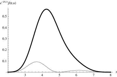
We have plotted the scalar curvature for this warp factor for and . Note that the behavior of the scalar curvature is opposite of the linear case because for the non-linear case the scalar curvature is regular for but diverges at infinity. Moreover, the curvature is positive around the origin and is negative for large distances.
Therefore, the geometry for the warp factor has a well-behavior in the origin but diverges asymptotically. Furthermore, asymptotically the warp factor satisfies
| (51) | |||
| (52) |
Then, for and the angular Einstein equation satisfies
| (53) |
However, since the scalar curvature diverges far from the brane, we can not conclude that the bulk converges to the space. Indeed, since the scalar curvature diverges at infinite and
| (54) |
whatever produces this geometry, the scalar curvature has a radial energy-momentum tensor component that diverges asymptotically. This feature contrasts a lot with the string-like geometry.

IV Scalar field in minimal coupling
Now let us study the localization of a scalar fields in the geometry analyzed so far. The action for scalar field minimally coupled to the gravity is
| (55) |
The equation of motion for the scalar field is given by
| (56) |
Let us assume that this scalar field is a product of a 4-component field with Poincaré symmetry and another scalar field living only in the 2-cycle of conifold, i.e.,
| (57) |
From Poincaré symmetry the 3-brane scalar field must satisfies the mass condition
| (58) |
Since , let us assume that can be expanded in Fourier series as
| (59) |
Using the ansatz yields
| (60) |
Equation is a Sturm-Liouville like equation. Further, let us looking for solutions that satisfy the boundary conditions
| (61) |
If we have two solutions of eq. , namely and , the orthogonality relations between them are
| (62) |
We can rewrite eq. (60) as
| (63) |
Note that equation (63) is similar to that found in string-like geometries [6, 7], regardless the conifold terms . Further, we can see from equation (63) that it is possible to add the conifold terms to the warp factors. Here we can choose two distinct paths. On one hand it is possible to study the resolution behavior directly in the warp factors. On other hand, we can study the localization in a factorized geometry, i.e., without the exponential warp factors . Besides, we could define an effective angular number which would depends on the point and on the resolution parameter.
IV.1 Massive modes
Let us simplify the equation (63) making the following change of variable
| (64) |
Since the radial metric component is a non-negative smooth function of , i.e., , so for a fixed , Thus,
| (65) |
and so is a smooth, monotonic increasing function of .
Using the change of variable in eq.(64) the equation (63) turns to be
| (66) |
In order to simplify further, let us write in the form
| (67) |
From equation (66), the function must obey
| (68) |
where
| (69) | |||||
This is a time-independent Schroedinger-like equation. We can study the localization of the scalar field by analyzing the behavior of the potential around a potential well. Returning to coordinate the potential can be written as
| (70) | |||||
The study of this potential provides graphic information about the possible stable solutions around a minimum.
IV.1.1 Linear warp factor
Now, let us analyze the case for the linear warp factor keeping the condition . The potential is given by
| (71) | |||||
We have plotted the potential for in the figure (9). For large values of the potential well decay exponentially. As two asymmetric minima arise far from the brane. However, for , the point turns to be an infinite potential well. Therefore, it is possible to find a localized solution of eq. (66). Indeed, the eigenfunction must satisfies the differential equation
| (72) |

.
For , which is valid for the singular cone () and for distant points (), the radial function satisfies
| (73) |
Note that eq. (73) differs from the string-like [6] equation for massive modes by the factor . For , eq.(73) converges to well-known equation of string-like defects [6]
| (74) |
and so asymptotically the field has the same features as in string-like geometry. For instance, the spectrum of mass has the same asymptotic behavior.
In order to study the behavior of massive modes near the brane let us take the limit , and therefore the equation for the radial component becomes
| (75) |
We can also use eq. (75) to study the asymptotic behavior of the eingenfunction for singular conifold whereas .
For , eq. (75) turns to be the string-like equation for massive modes [6]. Hence, the resolved conifold geometry resembles asymptotically and close to the brane the string-like geometry. Therefore, for or we have the well-known string-like solution
| (76) |
However, this solution in eq. (76) is not normalizable for . In order to normalize the field we can use a cut-off distance and apply the boundary condition in the point instead of the infinity. Then we take the limit and analyze the behavior of the mass spectrum. Since the solution of eq. behaves near and far the brane like the Bessel functions, for , the asymptotic mass spectrum must be of the form
| (77) |
On the other hand, expanding the exponential until first order yields
| (78) |
Therefore, this equation describes either the behavior of the field in the neighborhood of the brane or the asymptotic behavior of the eigenfunction for . Their solution is the product between an exponential function and the confluent hypergeometric function of second kind, namely
| (79) |
where, . The graphic of this function was plotted in the fig. (10).

IV.1.2 Nonlinear warp factor
Now let us study the solutions for the nonlinear warp factor. First, we have plotted the potential using several values of the resolution parameter and in the figure (11). For there is a potential well on the brane () and then there are massive modes trapped to the brane. Nevertheless, for , there is a potential barrier on the brane and there is only a potential well beside the brane. However, for a potential well appears again on the brane and thus there are localized states on the brane in the singular conifold.
The eigenfunction must satisfies
| (80) |
For we can expand the warp factor and its exponential around . This yields the equation
| (81) |
The solution for this equation is again a product between a exponential function and the hypergeometric confluent function. Its plot is shown in the figure (12).


For the eigenfunction satisfies
| (82) |
whose solution is
| (83) |
We have plotted the solution above in the figure (13). Note that the function is well defined on the brane but asymmetric in relation to the brane. Therefore, the eigenfunction for the singular conifold is localized on the brane. Besides, since the eigenfunction vanishes at infinity, the eigenfunction for is also localized.

IV.2 Massless modes
Now let us turn our attention to the massless modes ( or Kaluza-Klein modes). Considering and (which is called s-wave) [7], the radial equation (63) becomes
| (84) |
The constant function satisfies the equation above. Thus, this solution is said to be localized if its action is localized around the 3-brane, i.e., if its action have compact support. Since the equation (84) is a Sturm-Liouville equation and we are seeking localized functions that satisfy the asymptotic condition
| (85) |
we can find a spectra of eigenfunctions satisfying the orthonormal condition
| (86) |
Therefore, we can define the eigenfunction in flat space as
| (87) |
On the other hand, since
| (88) |
the zero-mode eigenfunction is
| (89) |
where
| (90) |
Again, the eigenfunction is quite similar to that found in refs. [6, 7] regardless the factor . We have plotted the zero-mode for some values of using the linear warp factor in the fig. (14) and for the nonlinear warp factor in the fig. (15). Since for every the function is integrable we can say that the massless field is localized on the brane even for the singular conifold case.


V Conclusion and perspectives
We have studied the localization of a scalar field on a 3-brane in a resolved conifold background of six dimensions, builded from a warped product between a 2-cycle of a resolved conifold and a 3-brane placed in the tip of the cone. We have chosen a geometry such that when the resolution parameter goes to zero or when we put the 3-brane far from the origin, we re-obtain the well-studied string-like geometries.
The use of the resolved conifold as a transverse space brought a very nice feature: an extension to the solution of the hierarchy problem using the resolution parameter . Indeed, in the Randall-Sundrum and string-like models, the ratio between the six-dimensional Planck mass and the four dimensional Planck mass depends only on the cosmological constant and on the tension of the brane . Since this parameter has a purely geometric origin it has opened the way to use another parameter-dependent manifolds like Eguchi-Hanson spaces, Taub-Nut, etc, as transverse spaces. Furthermore, using parameter dependent transverse spaces we could study the evolution and stability of the hierarchy between and through some mechanisms, for example, the conical transitions or the geometrical flux.
For a linear warp factor, the bulk geometry asymptotically approaches to the space () which is similar to the string-like geometry. Further, the massive modes have a family of potentials parameterized by the resolution parameter. For , the potential decreases exponentially and then it is not possible to have stable trapped states in the brane. As , two asymmetric minima appear around the 3-brane put in the point , but the potential reaches its maximum value on the brane. The respective eigenfunction is localized around the deepest minimum close to the brane. In the limit , the potential well turns out to be a infinite potential well in the brane and thus the eigenfunction is localized in the brane. Indeed, both for , and for we obtain the well-known solution for string-like geometry [6]. Besides, the massless modes was localized even for the singular case. Indeed, the action for a constant solution in this geometry has compact support and therefore is normalizable. The main difference between this conifold geometry and the standard string-like one lies on the parameterization of the potentials by a geometric factor. This parameterization provides the asymmetric minima potentials far from the brane. Therefore, the resolution parameter could be used as a filter of fields that can be or not be localized on the brane.
Using the nonlinear warp factor the scalar curvature diverges asymptotically and so the energy-momentum tensor is not restricted to points closed to brane which is in contrast to the string-like geometry. For the scalar field, the massive modes are trapped on the 3-brane even for the singular conifold. For the potential behaves like the standard volcano potential with a minimum on the brane. As two more local minima appear inside the global minimum and the minimum on the brane turns to be a maximum. Therefore, in the range is not possible localize the scalar field on the brane. In the same way that for linear warp factor, for the potential on the brane returns to be a potential well but now infinite. At last, the massless modes are localized for all values of . A difference between this geometry and the string-like one lies on the radial field solutions. Indeed, for string-like geometries the usual field solutions are Bessel functions and in this work we have found confluent hypergeometric functions that depend on two parameters and which are very sensible to variations on these parameters. This was expected since the field equation depends on the mass and angular number . Also, the field equation, through the geometry, depends on the resolution parameter . We argue that using other parameter-dependent geometries we could find more general solutions and study its stability.
We also argue that the successful localization of massless modes in the singular conifold for both linear and nonlinear warp factor might be related with the fact that in the conifold transitions, where we make singularities in the manifold, some fields become massless. Thus, this closed relationship between conical singularity and the spectrum of massless fields provides the localization of the massless modes in the singular geometry.
This work suggests many perspectives. Using the same geometry studied so far, we could study the localization of other fields in this scenario, like the vector, gravitational and spinor fields. Since these fields have more degrees of freedom than the scalar field the effects of asymmetry of the potential could be more relevant, for example, for the resonance of fermionic modes. Another way it could be use another parameter-depend geometries like the deformed conifold or even orbifold instead of the resolved conifold. Since these smooth conifolds are related with supergravity solutions that near horizon behaves like we could study the localization of fields where the transverse space are well-known solutions like the Eguchi-Hanson spaces or the Klebanov-Strassler throat. Furthermore, since we have parameterized the geometry we could study the stability of this geometry using some analytical method like Ricci equation, where the variable of the flux would be the resolution parameter. Since there is a relation between the resolved conifold geometry and the cigar-like geometry we could study the flux through a parameterized cigar geometry. On the other hand, we could use the geometry bulk used here to study other problems as the small value of the cosmological constant in the 3-brane and the supersymmetry breakdown.
It worthwhile to mention that even though we have studied the behavior of the field in that geometry we have not said how this geometry was generated. Hence, a next step could be deduce this geometry from some field and so to give a physical meaning to the resolution parameter.
The authors would like to thank the Brazilian agencies FUNCAP, CNPq and CAPES for financial support.
References
- [1] L. Randall and R. Sundrum, Phys. Rev. Lett. 83, 4690 (1999) [arXiv:hep-th/9906064].
- [2] L. Randall and R. Sundrum, Phys. Rev. Lett. 83, 3370 (1999) [arXiv:hep-ph/9905221].
- [3] J. W. Chen, M. A. Luty and E. Ponton, JHEP 0009, 012 (2000) [arXiv:hep-th/0003067].
- [4] A. G. Cohen and D. B. Kaplan, Phys. Lett. B 470, 52 (1999) [arXiv:hep-th/9910132].
- [5] R. Gregory, Phys. Rev. Lett. 84, 2564 (2000) [arXiv:hep-th/9911015].
- [6] T. Gherghetta and M. E. Shaposhnikov, Phys. Rev. Lett. 85, 240 (2000) [arXiv:hep-th/0004014].
- [7] I. Oda, Phys. Lett. B 496, 113 (2000) [arXiv:hep-th/0006203].
- [8] P. Candelas and X. C. de la Ossa, Nucl. Phys. B 342, 246 (1990).
- [9] B. R. Greene, D. R. Morrison and A. Strominger, Nucl. Phys. B 451, 109 (1995) [arXiv:hep-th/9504145].
- [10] J.Polchinski, String theory and beyond, vol.2, Cambrigde University press.
- [11] I. R. Klebanov and M. J. Strassler, JHEP 0008, 052 (2000) [arXiv:hep-th/0007191].
- [12] L. A. Pando Zayas and A. A. Tseytlin, JHEP 0011, 028 (2000) [arXiv:hep-th/0010088].
- [13] M. Cvetic, H. Lu and C. N. Pope, Nucl. Phys. B 600, 103 (2001) [arXiv:hep-th/0011023].
- [14] H. Firouzjahi and S. H. Tye, JHEP 0601, 136 (2006) [arXiv:hep-th/0512076].
- [15] T. Noguchi, M. Yamaguchi and M. Yamashita, Phys. Lett. B 636, 221 (2006) [arXiv:hep-th/0512249].
- [16] F. Brummer, A. Hebecker and E. Trincherini, Nucl. Phys. B 738, 283 (2006) [arXiv:hep-th/0510113].
- [17] J. F. Vazquez-Poritz, JHEP 0209, 001 (2002) [arXiv:hep-th/0111229].
- [18] E. Ponton and E. Poppitz, JHEP 0102, 042 (2001) [arXiv:hep-th/0012033].
- [19] A. Kehagias, Phys. Lett. B 600, 133 (2004) [arXiv:hep-th/0406025].
- [20] M. Cvetic, H. Lu and C. N. Pope, arXiv:hep-th/0002054.
- [21] R. Gregory and C. Santos, Class. Quant. Grav. 20, 21 (2003) [arXiv:hep-th/0208037].
- [22] B.Chow, P.Lu, L.Ni, Hamilton’s Ricci flow, Science Press, 2006.
- [23] B. de Carlos and J. M. Moreno, JHEP 0311, 040 (2003) [arXiv:hep-th/0309259].
- [24] G. Perelman, arXiv:math/0211159v1.
- [25] P.Topping, Lectures on the Ricci flow, London Mathematical Society, Lecture note series 325, Cambridge university press.
- [26] C. E. Fu, Y. X. Liu and H. Guo, arXiv:1101.0336 [hep-th].