INSTITUT NATIONAL DE RECHERCHE EN INFORMATIQUE ET EN AUTOMATIQUE
On the Coloring of Grid Wireless
Sensor Networks: the Vector-Based Coloring Method
Ichrak Amdouni — Cedric Adjih — Pascale Minet
N° 7756
October 2011
On the Coloring of Grid Wireless Sensor Networks: the Vector-Based Coloring Method
Ichrak Amdouni , Cedric Adjih , Pascale Minet
Theme : Networks and Telecommunications
Networks, Systems and Services, Distributed Computing
Équipe-Projet Hipercom
Rapport de recherche n° 7756 — October 2011 — ?? pages
Abstract: Graph coloring is used in wireless networks to optimize network resources: bandwidth and energy. Nodes access the medium according to their color. It is the responsibility of the coloring algorithm to ensure that interfering nodes do not have the same color. In this research report, we focus on wireless sensor networks with grid topologies. How does a coloring algorithm take advantage of the regularity of grid topology to provide an optimal periodic coloring, that is a coloring with the minimum number of colors? We propose the Vector-Based Coloring Method, denoted VCM, a new method that is able to provide an optimal periodic coloring for any radio transmission range and for any -hop coloring, . This method consists in determining at which grid nodes a color can be reproduced without creating interferences between these nodes while minimizing the number of colors used. We compare the number of colors provided by VCM with the number of colors obtained by a distributed coloring algorithm with line and column priority assignments. We also provide bounds on the number of colors of optimal general colorings of the infinite grid, and show that periodic colorings (and thus VCM) are asymptotically optimal. Finally, we discuss the applicability of this method to a real wireless network.
Key-words: Graph coloring, wireless sensor networks, grid, periodic coloring, Vector-based Method, valid coloring, optimal coloring, number of colors bounds.
Coloriage des réseaux de capteurs en grille: La méthode de coloriage basée sur les vecteurs
Résumé : Le coloriage des graphes est utilisé dans les réseaux sans fil afin d’optimiser les ressources du réseau: la bande passante et l’énergie. Les noeuds du réseau accèdent au médium en fonction de leur couleur. L’algorithme de coloriage a la charge d’assurer que les noeuds intereférents n’aient pas la même couleur. Dans ce rapport de recherche, nous nous concentrons sur les réseaux de capteurs sans fil ayant une topologie en grille. Comment un algorithme de coloriage peut profiter de la régularité de cette topologie pour réaliser un coloriage périodique optimal, c’est à dire un coloriage avec le nombre minimal de couleurs? Nous proposons la Méthode des Vecteurs, notée VCM, une nouvelle méthode qui est capable de fournir un coloriage à sauts, périodique et optimal quelque soit et quelque soit la portée radio. Cette méthode consiste à déterminer quels noeuds de la grille peuvent utiliser la même couleur sans créer des interférences entre ces noeuds tout en minimisant le nombre de couleurs utilisées. Nous comparons le nombre de couleurs utilisées par la Méthode des Vecteurs, à celui obtenu par un algorithme distribué qui affecte les couleurs selon la priorité donnée par la ligne ou la colonne. Nous fournissons aussi des bornes sur le nombre de couleurs des coloriages généraux optimaux de la grille, et prouvons que les coloriages périodiques (et donc VCM) sont asymptotiquement optimaux. Enfin, nous discutons l’applicabilité de cette méthode à un réseau sans fil réel.
Mots-clés : Coloriage des graphes, réseaux de capteurs sans fil, grilles, coloriage périodique, Méthode des Vecteurs, coloriage valide, coloriage optimal, bornes sur le nombre de couleurs.
1 Context and motivation
Node coloring consists in assigning colors to nodes using a minimum number of colors such that two interfering nodes do not have the same color. It has been proved that the 1-hop coloring problem in [2] and more generally the -hop node coloring problem with an integer is NP-complete [3, 4]. That is why, approximation algorithms are adopted. Among them, FirstFit [8] assigns to the uncolored node with the highest priority the first available color. Unfortunately, the number of colors obtained depends on the node coloring order given by the priority. A whole class of results expresses properties related to the worst-case performance of approximation algorithms: they typically prove that, for any input graph of a given family, the coloring obtained by a given algorithm uses at most times the optimal number of colors. Such an algorithm is denoted an -approximation algorithm.
Many coloring algorithms have been designed to be used in wireless networks to make the medium access more efficient. Among them, we can cite TRAMA [9], FLAMA [10], ZMAC [11] which is based on the DRAND [12] coloring algorithm, TDMA-ASAP [13], FlexiTP [14] and SERENA [17]. In short, time slots are assigned per node color: two nodes with the same color can transmit in the same time slot without interfering.
In this research report, we focus on wireless sensor networks with grid topologies. These topologies are regular.
Wireless sensors organized according to a grid topology are
a natural choice and exist in many real applications.
Often, the grid organization is easy to deploy,
and is efficient in terms of coverage, connectivity and management.
For instance, a grid topology is one of the best methods to ensure sensor
coverage for surveillance [5, 6].
It also helps to collect measurements with a uniform spatial sampling such as for
instance in precision agriculture and irrigation as in [7]: when physical phenomena are numerically modeled, measurements from a grid pattern may be a direct input or directly compared to the output of equations solved with the finite element method on a grid — without requiring additional sensor localization and numerical measurement interpolation.
Given such grid topologies, the question (and our problem statement), is:
what is the method to color grids while maximizing the color reuse?
Naturally, a first step towards answering the question, is to apply existing
algorithms to a sample of grids and analyze the output for some sample topologies.
| Grid size | priority assignment | colors | colors |
| for range = 1 | for range = 2 | ||
| 10x10 | line or column | 8* | 30 |
| diagonal | 8* | 28 | |
| distance to origin | 8* | 30 | |
| random | 13 | 36 | |
| 20x20 | line or column | 15 | 33 |
| diagonal | 8* | 29 | |
| distance to origin | 8* | 30 | |
| random | 14 | 41 |
We have performed simulations of a 3-hop coloring, because 3-hop coloring is needed when broadcast and immediate acknowledgement of unicast transmission are required.
The algorithm colors nodes according to their priority order among their neighbors up to -hop. Node priority is given by one of the following heuristics: the position of the node in the line, column, diagonal, its distance to the grid center or random.
Results are summarized in table 1. The ’*’ symbol highlights the optimality of the number of colors used. The reader can refer to [4] for the proof of the optimal number of colors needed to color some grids with various transmission ranges. Different radio ranges are simulated.
Mostly, we observe that no priority assignment tested provides the optimal number of colors for any grid size and any radio range.
This prompts the following questions: Does a priority assignment exist in grid topologies such that the number of colors does not depend on node number but only on radio range?
Is it possible to take advantage of the regularity of grid to design a -hop coloring algorithm able to find the optimal number of colors for any grid with any transmission range value?
Moreover, does a periodic color pattern that can tile the whole topology for a given radio range, exist? What is the optimal number of colors? Is the optimal number of color reached by periodic colorings?
In this research report, we answer these questions by proposing a coloring method,
the Vector-Based Coloring Method, denoted VCM which provides an optimal and valid coloring of grids.
The research report is organized as follows. In Section 2, we introduce some definitions and notations. We present the problem statement and give an intuitive idea of VCM and introduce its main components. In Section 3, we focus on periodic coloring. In Section 4, we consider periodic colorings where any color is periodically reproduced, and show how VCM computes the color of an node in the grid. In Section 5, we restrict or study of periodic coloring to valid ones. We propose two methods to check the validity of periodic coloring. Section 6 allows us to characterize an optimal coloring and give upper and lower bounds on the number of colors, and shows that periodic colorings (and therefore VCM) are asymptotically optimal when the radio range increases11 1 showing that specifically for grids, there are better techniques than already known general -approximations (even for unit disk graphs, such as [20]), since here when . We then show how to reduce the research space of the generator vectors produced by VCM in order to reduce the complexity of VCM that we evaluate (which is polynomial time). We conclude this section by giving the method to find the optimal valid generator vectors. In Section 7, we summarize by giving rules to apply VCM in practice. Results obtained by VCM are given in Section 8 and compared with those obtained by different heuristics. Finally, in Section 9, we discuss how to apply VCM in real wireless sensor networks. We conclude in Section 10. In the Annex, the reader will find some mathematical results and grid properties useful for grid coloring.
2 Problem Statement and Overview
2.1 Notations, Definitions and Assumptions
In the remaining of this research report, we use the following notations:
- •
denotes a vector of extremities the nodes and .
- •
denotes the norm, or length of the vector , and the euclidian distance between nodes and .
- •
is the determinant of the two vectors.
- •
denotes the scalar product of the vectors.
- •
denotes the lattice having as a base the vectors . We call and the basis (or generator) vectors. is the fundamental parallelotope associated to . In 2 dimensions, is a parallelogram. Moreover, the number of nodes in called lattice determinant is given by . These notations and definitions are adopted from [15]. We also denote the fundamental parallelotope translated at node .
- •
For in , with , we denote "x modulo y" the integer z in such that we have
Moreover, the following definitions and assumptions are used:
- •
Nodes: The nodes are disposed in a grid. Without loss of generality, we assume that the grid step is , hence the set of nodes is identified by .
- •
Neighborhood: denotes the radio range and is a real number . The underlying assumption is a unit disk model, assuming that nodes and can communicate if their euclidian distance is lower than and are able to communicate directly in both directions. Hence, the set of neighbors of a node is:
. - •
Coloring: A coloring is a mapping from the nodes to a set of colors, identified with the set of integers , with a positive integer.
- •
Valid Coloring: a coloring is said to be a valid -hop coloring, with an integer , when all nodes that are less or equal to -hop away are assigned different colors.
- •
Periodic Coloring: A coloring is denoted “periodic” if the set of nodes with the same given color, is the lattice for some fixed vectors , of , after it is translated by some amount. In this paper, we consider a “strict” definition of periodicity because colors might otherwise be periodically repeated with a pattern generating more than a single lattice for instance.
2.2 Problem Statement
Our general goal is the following: Find a valid -hop coloring of
the nodes of the infinite grid , with a minimal number of colors for .
Because the set of colorings of is infinite, in this paper we
restrict ourselves to colorings exhibiting a periodic color pattern
(following the definition of periodic coloring of section 2.1).
Problem Statement: Find one of the valid periodic -hop colorings with the minimum number of colors for .
2.3 Overview
In this paper, we propose the periodic Vector-Based Coloring Method, denoted VCM that answers the problem
statement in polynomial time. This method consists in producing a periodic coloring obtained by tiling a color pattern. This color pattern is generated by two vectors verifying some conditions that will be detailed in the paper.
As illustrated in Figure 1, VCM is composed of the following components:
C1. VCM-NCC A periodic coloring based on two generator vectors. This component determines how any sensor node selects its color.
C2. VCM-VC An algorithm to check the validity of the periodic coloring: the VCM incorporates two methods to verify the validity of the coloring for a given couple of generator vectors.
C3. VCM-OVS An algorithm to search for optimal generator vectors, that is, yielding the minimum number of colors.
Indeed, we limit the set of candidate vectors to find the vectors providing the optimal number of colors.
2.4 Intuitive Idea
The intuitive idea of the method is as follows. As the grid topology presents a regularity in terms of node position, VCM produces a similar regularity in terms of colors and generates a color pattern that can be periodically reproduced to color the whole grid.
Our aim is to find such a color pattern that minimizes the number of colors used. More precisely, given a colored node , we determine where its color can be reproduced.
The method starts by the choice of two
vectors and such that and use the same color as . Of course, the vectors must provide a valid -hop coloring.
The color pattern is given by the set of colors in the finite parallelogram translated at . Hence, the color of is repeated also at any node where is a linear combination of and .
In the Sections from 4 to 6, we detail the components of VCM.
3 Periodic Coloring
Figure 2 presents an example of a periodic 3-hop coloring of a grid with a transmission range .
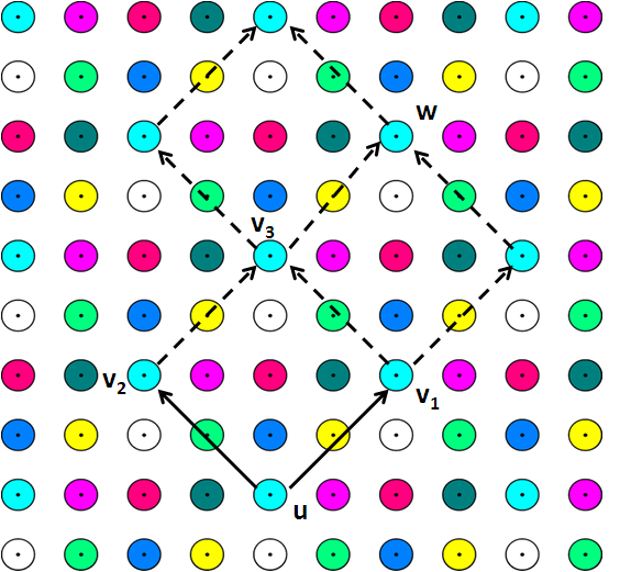
The principles of the periodic coloring are:
P1. (Generator vectors) The two vectors and , if linearly independent, generate the parallelogram of the color pattern.
P2. (Parallelotope color unicity) Inside , there is no color reuse.
P3. (Lattice color repetition) Because the periodic coloring is obtained by repeating the color pattern, the nodes
such that is a linear combination of and have the same color as . Precisely, the set of nodes having the same color as forms a lattice of with generator vectors and : the vector can be written as with and in .
P4. (Coordinate-based color computation) The grid can be seen as a tiling with the pattern . Thus, each node belongs to its own parallelogram, and has coordinates relative to this parallelogram. Consequently, has the same color as any node having the same coordinates in its own parallelogram.
To be applied to a wireless sensor network, these principles have to be enhanced. For instance, since nodes having the same color can simultaneously access the wireless medium, validity of the coloring must be verified. Moreover, to ensure an efficient usage of the bandwidth, the number of colors used should be minimized. These criteria are taken into account in our work and progressively introduced in the paper.
In the following we detail the components of VCM. As previously said, we only consider grid colorings that periodically reproduce a color pattern.
4 VCM: Node Color Computation (NCC)
4.1 Assigning Colors to Nodes
The node color computation (NCC) component of the VCM method takes as parameters two generator vectors , (computed as in Section 6). Let and be their coordinates and let .
Here we define two methods to compute the colors.
Actual computation on an example is provided in Section 4.3.
4.1.1 Method NCC1
VCM assigns the color of a point based on its coordinates by computing first the integer quantities as in System (4.1.1),
{System}
c_1(w)= (xy_2 - yx_2) modulo d
c_2(w)= (-xy_1 + yx_1) modulo d
and then using a bijective mapping between the couple and a color .
Remark 1
Defining as , instead of the definition in (4.1.1), would be more symmetrical compared to , and would yield identical results (as it is a trivial transformation: ).
Remark 2
In the remaining of this report, we will assume that without loss of generality: indeed, if , it is sufficient to use the vectors instead of and the results are similar ; notice that , etc. (hence change of sign of is equivalent to an origin symmetry of the coloring). This avoids minor technicalities on the definition of the modulo, integer part, fractional part, when numbers are negative (for which definitions are not universal).
Property 1
With the previous coloring VCM-NCC1, it is indeed possible to define a bijection from to . Moreover, the coloring verifies principles P3 and P4 defined in Section 3.
Proof: We assume that without loss of generality (see Remark 2). We need to prove that the set has cardinality and that the set of nodes with the same color is exactly the lattice translated at .
Let be a grid point of coordinates . Performing a change of vector basis in from to ,
the new coordinates of W in verify and
{System}
α=
det(w,u
2
)
d
β=
det(u
1
,w)
d
with .
Let and be the integer parts of , i.e.,
and .
For arbitrary nonzero integers , with also , we have the identity:
.
Thus 4.1.1 becomes:
{System}
α= α’+
det(w,u
2
) modulo d
d
= α’ +
c
1
(w)
d
β= β’+
det(u
1
,w) modulo d
d
= β’ +
c
2
(w)
d
Let the point with coordinates .
is on the lattice since are integers,
and observe that is in fact inside the parallelogram of the lattice
placed at node (i.e. inside the parallelogram defined
by the points of the lattice:
, , , ). Then (4.1.1)
means simply that are the
coordinates of relative to this parallelogram
(with the basis vectors ).
Since there is a bijection between the set of coordinates of nodes in a parallelogram of and the nodes themselves; and since are these coordinates, we have the two properties: 1) there are exactly possible values of (because there are exactly nodes in the parallelogram), and 2) no two nodes inside the parallelogram have the same values since these are their coordinates, relative to one vertex of the parallelogram.
Lemma 1
With the color computation given by the System 4.1.1, the color of the node is repeated at the nodes with coordinates verifying: , for some .
Proof: Actually, by construction, the color of a node is given by its coordinates relative to the parallelogram it belongs to. Hence, the color of any node is reused at nodes , such that for all , which have the same relative coordinates.
We deduce that VCM-CC1 provides a coloring that is really consistent with the principle of the method as described in Section 3.
4.1.2 Example of bijection for NCC1
One of the steps of the Method NCC 1, is that a bijection needs to be established between the set of values and the set of colors : an example of bijection is provided in this section.
A bijection can be constructed by computing the values of for any node in in a list, sorting the list by lexicographical order, and, finally, setting the color associated with a couple to be its index in the sorted list minus 1.
Example: if appears as the item of the sorted list [as it can be proved it will], the color assigned to that couple is . Then, for instance, for the point of coordinates , in other terms , we have and therefore the color assigned to is .
Note that, from a pure implementation point of view, it may be difficult to enumerate exactly the points of , but then, instead, it is sufficient to enumerate all the nodes in a superset, the bounding box of , itself computed from its four vertices , , and . Computing the set of values for the points in the bounding box, will yield all possible values for any .
4.1.3 Method NCC2
Method 2 is derived from the first method ; the difference is that it also establishes a direct bijection (and hence avoids the need for constructing a bijection as in section 4.1.2): it proceeds to a direct computation of the color based on the node coordinates without computing the colors of the other nodes on the parallelogram.
As for Method 1, we assume that we are given two generator vectors with coordinates and , and that we are computing the color of node of coordinates .
In addition to the notations and definitions used previously, we introduce the following ones:
- •
is the greatest common divisor of ; . Similarly, , with the convention
- •
is the vector and is the vector . Notice that the coordinates of and are coprimes.
- •
Let . We have:
- •
Let be the coordinates of the node relative to the basis , when performing a change of basis in from to . We have: and .
- •
Let
- •
Let
- •
Let
Using the notations mentioned above, a color of a node with coordinates is equal to (1) which is an integer in
As in remark 2, we now assume that without loss of generality.
The idea of the method VCM-NCC 2 is as follows:
- •
In method VCM-NCC 1, we did not identify nor did make use of the special structure of , which is in fact a subgroup of ; hence we did not provide an explicit mapping from to . This is the problem that method 2 addresses:
- •
In method VCM-NCC 2, by dividing the vectors and by the respective gcd of their coordinates, we obtain vectors , and we find that applying method VCM-NCC 1 with these vectors, the set of values has good properties, allowing the construction of a direct bijection (see lemma 2).
- •
However using method VCM-NCC 1 with vectors yields a coloring of repeated by translation by and ; whereas we wanted a coloring repeated by translation by and (which are larger). Notice that the problem here is that method VCC-NCC 1 with generator vectors is quite possibly an invalid -hop coloring of , even if are vectors defining a valid -hop coloring. For this reason, method VCM-NCC 2 constructs a coloring based on method VCM-NCC 1, but modified, by tiling the parallelogram several times inside the parallelogram and changing the colors in each internal tile (see figure 3).

Method 2 is in fact the combination of two functions; with:
- •
The first one, , from to , which associates to the value .
- •
The second is bijection from to by transforming ; note that by definition.
The transformation is obviously a bijection from its domain to its codomain22 2 informally, it is similar to a transforming the time of the day expressed as h:m:s – hour minutes seconds – into the time of the day expressed as seconds from midnight as , and therefore the crux of method VCM-NCC 2 is the function .
We start with the following lemma for the function , which is in fact :
Lemma 2
Let be the value “” obtained when applying method
VCM-NCC 1 with generator vectors , and define
similarly.
Then the function is a direct coloring of the
nodes , where the color is in .
This lemma establishes that for the specific generator vectors ,
computes directly a color and is essentially redundant.
Proof: We prove this lemma in two steps: (S1) proves that the set covers exactly integers in , and (S2) the coloring provided by has the same properties as . To prove this, we prove that there is a bijection between and .
(S1) Consider the vector . By definition, is the gcd of its coordinates . Applying Bézout’s identity ([21]), there exist integers33 3 this is even true when or with our convention , such that:
| (2) |
Let be the vector of coordinates and let be the coordinates of (recall that is defined as ). Because , we have and and hence equation (2) becomes:
Since is a linear map: , etc. and by applying it to , we get exactly:
.
(S2) Let be the set . From properties previously proven for method VCM-NCC 1 (including property 1), we know that there exists a bijection from to the set ; in other words, that its cardinality verifies .
Now consider the projection . The previous relation shows that hence it is a bijection because it is surjective between two sets of cardinality .
Therefore we have explicitly found one bijection (precisely: ) compared to the method VCM-NCC 1 where we only established the existence of such a bijection. The end result, is that when applying VCM-NCC 1 with the generator vectors and with this bijection , the color of a node is . The coloring provided by inherits from VCM-NCC 1, all the properties listed in Section 3.
The next step is to build a coloring repeated by translation of and , from the coloring VCM-NCC 1. As illustrated in Figure 3, the idea is that are the basis of the parallelogram that can be tiled to cover the parallelogram ; this is possible because and (where and are integers). Inside a parallelogram , the nodes are assigned the same color as given by VCM-NCC 1 with , except that an offset is added, depending in which tile the node is located.
Concretely, in Figure 3, the parallelogram at the right side of the picture is tiled with smaller parallelograms which are versions of , filled by different shades of gray. The nodes in one small gray parallelogram are allocated the colors ; the ones of the next small gray parallelogram are allocated the colors ; and generally the nodes of the parallelogram are allocated the colors . The actual coloring is then something like the colored nodes at the left of the Figure 3.
Thus, the central idea is to identify in which sub-parallelogram a node is located: this is given by , which are in fact the coordinates of the smaller parallelogram on the basis counted relative to the larger parallelogram. For instance, in Figure 3, the point is inside a sub-parallelogram of coordinates relative to the bigger parallelogram.
This is the informal idea behind the quantities defined previously: in the following lemma, we now prove formally that VCM-NCC 2 is a coloring satisfying the desired properties.
Lemma 3
The coloring provided by the method VCM-NCC 2 satisfies the principles P1, P2, P3 and P4 from Section 3.
Proof:
Almost all the properties can be derived from identifying the set of nodes with identical colors.
Let and be two nodes with the same color, hence, with . Because and is a bijection, this implies that
| (3) |
The part implies that and have the same color in the method VCM-NCC 1 applied with vectors , therefore, by properties of this method:
Let us decompose as quotient and remainder modulo (resp. , modulo ): and where , and .
The previous equality becomes:
| (4) |
Now developing the part from (3), we get:
Which equality is true depends on which one of and has the largest fractional part. Assume it is , then we have:
The opposite is true: if verify this equality, , and then one can easily check that and similarly:
Likewise and thus finally , that is, the two nodes of coordinates and have the same color.
As a result, we have established that the nodes with identical colors are exactly the points located on a lattice generated by vectors . This is exactly the principle P3, and actually implies the principles P1, P2 and P4.
Remark 3
In this section, we selected as . Alternatively, one could select . Notice also that once the choice is made, lemma 2 does not require that coordinates are coprimes for both vectors and . Indeed, for the choice , (respectively ) only (respectively ) is required to have coordinates that are coprime.
4.2 Computing the Number of Colors
The number of colors used in a periodic -hop coloring is given by the next Property.
Property 2
For any node , the color pattern defined by the two generator vectors and meeting the aforementioned principles contains exactly colors where and are the coordinates of and .
Proof: By definition, no two nodes within the parallelogram defined by and use the same color. Hence the number of colors is equal to the number of nodes in this parallelogram. Moreover, as we said, the number of nodes in , called lattice determinant, is equal to the absolute value of det [15]. Hence the property.
4.3 Example of Color Calculation
In this section, we illustrate the color calculation, using the example of Figure 3.
In Figure 3, we have the following coordinates for :
- •
and
- •
Applying VCM-NCC 1 with the generator vectors , we get:
- •
Number of colors
- •
- •
Using the example bijection of Section 4.1.2, is the value in the sorted list of possible values, hence color
Applying VCM-NCC 2 with the generator vectors , we get:
- •
Number of colors
- •
and then
- •
and then
- •
, ,
- •
Color of :
For reference, the colors are computed internally from the coordinates on different basis: and
5 VCM: Validity Check (VC)
As defined previously, a -hop coloring algorithm is valid if and only if no two nodes that are at less or equal to -hop from each other use the same color.
The node color computation algorithm of VCM (described in Section 4) takes as input two generator vectors , and , and gives the color of each node. In this section, we will assume that such two vectors are given and fixed, and we present two methods for checking beforehand whether the coloring induced by these vectors is a valid coloring.
5.1 Method VC1: Verification around Origin
For each node in the -hop neighborhood of the origin node , we compute the color of this node based on the given generator vectors and . If has the same color as , then we conclude that the vectors and do not provide a valid coloring. Otherwise, if the color of , is not repeated at any point in its -hop neighborhood, then the coloring is valid.
The idea of Method 4 is based on the following fact, proven in this section: if there is a color conflict between any two nodes and in ( and have the same color despite they are at less than or equal to hops), there will be a color conflict in the -hop neighborhood of the origin .
We set .
Lemma 4
If two nodes and with coordinates , in have the same color, then the color of the origin node is repeated at the node of coordinates .
Proof: The functions computed from System 4.1.1 are actually linear modulo . That is, if is the node with coordinates , and is the vector of nodes extremities the origin and , we get: . Hence, if we have . This is true also for , hence the lemma.
Theorem 1
If none of the nodes inside the -hop neighborhood of the origin node has the same color as itself, then the coloring is valid.
Proof: By contradiction: assume that the coloring is invalid, which implies that two nodes at less or equal to hops have the same color. Then from Lemma 4, the node such as has the same color as . Notice that the distance in terms of hop number between and is the same as the distance between and . Hence we have found a color conflict between and a node which is at less than hops from . Hence the theorem.
Theorem 1 proves that Method VC1 is a correct method for checking whether two generator vectors yield a valid -hop coloring.
5.2 Method VC2: Verification in a Few Points
Method VC1 requires
verifications when . In the following, we propose Method VC2, usable when and requiring only a bounded number of verifications. Method VC2 performs a check on a few nodes on the lattice to guarantee that the -hop coloring associated to is valid. This method is based on Gauss lattice reduction [16] (see the Annex for more details): and should be first reduced,
and hence verify the Equations (11.1).
The nodes with the same color as the origin are on the lattice : this method verifies that these nodes are at least -away from , in which case the coloring is valid. However, not all grid nodes need to be checked. It is sufficient to check only nodes in with coordinates on the basis , such that and , with . The coloring is valid if and only if these nodes are strictly more than hops from the origin node.
This method is based on the following theorem.
Theorem 2
For , the coloring provided by two reduced vectors is valid if and only if:
for all integers verifying ,
and ,
the node with coordinates on the basis
is at strictly more
than hops from the origin node , where .
Proof: The property comes from the fact that the points on the lattice
are “far” from the origin node, because the vectors are reduced.
Indeed, Lemma 9 (see the Annex) means that any node on the lattice with coordinates , with or can reuse the color of the origin node because they are at strictly more that -hop from (provided that the points of coordinates or are themselves strictly more than -hop away from ). Hence, to check the validity of the coloring provided by VCM, it is necessary and sufficient to check that for all and , nodes of coordinates , in the lattice are strictly more than hops away from the origin of the lattice.
This check includes checking the validity of and themselves
(cases and )
Notice that for dense grids (), . This small bound reduces the set of nodes to be checked in order to verify the validity of the coloring for given vector candidates.
In fact for , that is for , we have , hence only points need to be checked (considering symmetries): (with ), (with ), (with ), (with ).
6 VCM: Optimal Vector Search (OVS)
To achieve an optimal spatial reuse, the coloring algorithm should minimize the number of colors used. For VCM, our aim is to judiciously choose the generator vectors and in order to reduce the number of colors used to color a grid. However, by default, the infinite lattice is a possible set for candidate vectors. So, to find the optimal vectors in a small set, our approach is as the following:
- •
We determine the upper and lower bounds on the number of colors needed in a -hop coloring of the grid, for .
- •
Because for any couple of initial generator vectors, reduced vectors always exist, it is sufficient to search for some optimal vectors in the space of reduced vectors defined by System (11.1).
We will show in Section 6.2 how to bound the set of candidate vectors using the properties of lattice reduction and the upper and lower bounds on the number of colors to decrease
the complexity of the search for the optimal vectors.
6.1 Bounds on the Number of Colors in Colorings
In this section, we prove that the number of colors of optimal colorings when is shown to be asymptotically , from the combination of two bounds.
6.1.1 Lower Bound
For the lower bound, we have the following theorem that is valid for any coloring, not just periodic colorings. It uses known results on circle packings.
Theorem 3
The number of colors required to color an infinite grid with is at least .
Proof: Consider -hop coloring of the grid . Consider a fixed color , and now let be the set of nodes having this color.
We first establish a lower bound of the distance of nodes in . Let us define . Consider two nodes of . By contradiction: if their distance verifies , from Lemma 6, they would be at most -hop away, contradicting the definition of a -hop coloring. Therefore, all nodes of are at a distance at least from each other.
Now consider the set of circles of radius and whose centers are the nodes of . The fact that any two nodes of are distant of more , implies that none of the circles in overlap. Hence is a circle packing by definition. From the Thue-Tóth theorem [18, 19] establishing that the hexagonal circle packing is the densest packing, with a density of , we deduce that must have a lower or equal packing density. This implies an upper bound of the density of set of centers of the disks of .
Because each color yields a set of nodes with at most this density, it follows a lower bound of the number of colors that is the inverse of this quantity, hence the theorem.
6.1.2 Upper Bound
For an upper bound, when , we construct explicitly a periodic coloring; more precisely we construct two vectors yielding a valid coloring with VCM. As a result, optimal colorings and optimal periodic colorings must have a number of colors which is lower or equal.
Because the vectors constructed yield lattices which are close to hexagonal lattices (when ), and because it happens that hexagonal lattices yields the densest packing (as used in the proof of theorem 3), the upper bound will be somewhat “close” to the previous lower bound.
We have the following theorem:
Theorem 4
The number of colors required to color an infinite grid is at most .
Proof: We proceed with a constructive proof, exhibiting two valid vectors which yield the result, using an approximation of an hexagonal lattice.
Figure 4 illustrates how some points and are constructed.
- •
Starting from the point , the line with an angle with the horizontal line is considered, and its intersection with the circle of radius yields the point .
- •
Next, the closest point of on the grid having higher coordinates and than is sought and is with coordinates .
- •
Then with coordinates is selected with .
Notice that by construction , and we have a valid choice of vectors and .
Denote the coordinates of . By construction: and , hence: . Moreover,
Consequently, we can write , the number of colors in the associated coloring as:
Remark 4
An alternate, simpler, choice of vectors is to compute the integer , and select the vectors with coordinates and . The number of colors is higher than for the near-hexagonal previous vectors (it is ), hence the vectors cannot yield the result of the next section, but the vectors can be used for an upper bound when .
6.1.3 Asymptotic Number of Colors
Theorem 5
The number of colors of an optimal periodic -hop coloring for a fixed verifies:
when .
Corollary 1
Theorem 5 is true even considering periodic and non periodic colorings.
Proof: A periodic coloring is a special case of general coloring (including periodic and non periodic). Hence, the optimal number of colors in general coloring is less than or equal to .
Corollary 2
VCM is asymptotically optimal even considering all possible valid colorings (even non-periodic). In other terms VCM is an -approximation of the optimal coloring(s) of the grid with some verifying (precisely: ) when .
Proof: VCM will find vectors with better or equal performance than those in Theorem 4. Indeed, in the worst case, these generator vectors for the “near-hexagonal” lattice will be selected by VCM.
6.2 Finding Optimal Vectors
The complexity of VCM lies in the generator vectors computation and in their validity check. In this section, we show how to limit the set of candidate vectors.
Let be two candidate vectors and be the angle between them. We search (respectively ) the lower and upper bounds of the length of (respectively ).
1. Considering a coloring, the vectors and must be valid. According to Lemma 6, we have:
| (5) |
2. As we said, in order to reduce the set of candidate generator vectors, we reduce the size of these vectors by using the lattice reduction algorithm of Gauss. A consequence of Gauss property 11.1 is that: , and hence:
| (6) |
3. As shown in Theorem 3,
.
It results: Using 6, we get:
| (7) |
And as , from 7 we have:
| (8) |
We now separate the cases where and
6.2.1 Case
To summarize, the two generator vectors should verify for :
{Equation}
l_1_min < |u_1| ≤l_1_max and
l_2_min < |u_2| < l_2_max
with:
{System}
l_1_min = h(R-
2
)
l_1_max =
2
3
S_h
l_2_min = h(R-
2
)
l_2_max =
2
3
S
h
h(R-
2
)
In practice, to compute the two generator vectors, we determine the upper and the lower bounds of the coordinates of , and using the System 6.2.1. Notice that we can search the vectors in the half plane , because if and are generator vectors, then their symmetric vectors with respect to () axis are also generator vectors. Consequently, we have:
-l_1_max ≤x_1 ≤l_1_max
0 ≤y_1 ≤l_1_max
and
{System}
-l_2_max ≤x_2 ≤l_2_max
0 ≤y_2 ≤l_2_max
6.2.2 Case
We use . In addition, we can use the bound implied by the vectors proposed in Remark 4, that is: , which replaces for the computation of . Then, instead of a fixed bounds for and , we propose a bound depending on , by using (7) we have: , and because we have: . Hence:
0 < |u_1| ≤hR+1
|u_1| ≤|u_2| ≤
2
3
(hR+1)
2
3 |u
1
|
6.2.3 Method OVS
To find the optimal vectors, we define Method OVS.
1. The first step is to search the initial set of generator vectors and . is the set of vectors having as coordinates the integers and verifying System 6.2.1 if
and System 6.2.2 if .
2. Now, the set should be filtered to keep only reduced and valid vectors. Indeed, for each couple of vectors in , we should verify:
2.1. are reduced, that is they verify System 11.1.
2.2. to check the validity of the coloring, two cases are possible:
2.2.1 if apply Method VC2.
2.2.2. otherwise, apply Method VC1.
3. After the step 2, we obtain the set of valid reduced vectors. Now, the optimal vectors are the vectors having the smallest absolute value of their determinant.
Notice that the search of the optimal vectors can be done by a central unit, that distributes the vectors to all nodes. It is also possible that each node in the grid computes the two generator vectors.
We can now evaluate the complexity of VCM that lies in the generator vectors computation and in their validity check.
Theorem 6
Depending on VC method, VCM complexity is in for Method VC1 and for Method VC2.
Proof: The vector search phase is in for each vector. The validity check is in for Method VC1 and for Method VC2.
7 Summary: How to Apply VCM in Practice
This section summarizes the previous sections. In practice, to apply VCM, we start from a set of sensor nodes arranged as a two-dimensional
lattice (identified by their integer coordinates).
In reality, in an actual network, the set of neighbors will not be exactly
given by the set of nodes within a fixed range . However, notice that
a valid -hop coloring for a given , is also a valid -hop coloring for
(although likely non-optimal). Hence, we start by selecting the value of , a radio range such as two nodes at a distance greater than are never neighbors
(may be using measurements or neighborhood detection), and a value .
Then, each node proceeds as follows:
1. Find the optimal valid vectors using the Method OVS.
2. Each node computes its color by applying either VCM-NCC 1 or VCM-NCC 2.
We can notice that VCM allows each node to know its color in a single round.
8 Coloring Results with VCM
Note that further examples of colorings are available externally at [22].
8.1 Examples of Vectors
Table 2 gives for different radio ranges two vectors generating the optimal periodic pattern as well as the minimal number of colors obtained by a periodic pattern, for both a 2-hop coloring and a 3-hop coloring. The ’*’ symbol highlights the optimality of the number of colors used.
| Radio | 2-hop coloring | 3-hop coloring | ||||
|---|---|---|---|---|---|---|
| range | vector1 | vector2 | colors | vector1 | vector2 | colors |
| 1 | (2,1) | (-1,2) | 5* | (2,2) | (-2,2) | 8* |
| 1.5 | (-3,0) | (0,3) | 9* | (4,0) | (0,4) | 16* |
| 2 | (3,2) | (-2,3) | 13* | (4,3) | (-3,4) | 25* |
| 2.5 | (4,3) | (-1,5) | 23* | (5,5) | (-7,2) | 45* |
| 3 | (5,3) | (-1,6) | 33* | (7,5) | (-8,4) | 68* |
| 3.5 | (5,4) | (-6,3) | 39* | (8,5) | (-8,5) | 80* |
| 4 | (7,3) | (-6,5) | 53* | (8,8) | (-11,3) | 112* |
| 4.5 | (9,2) | (-6,7) | 75* | (13,3) | (-9,10) | 157* |
| 5 | (9,4) | (-1,10) | 94* | (14,4) | (3,15) | 198* |
| 5.5 | (9,6) | (-1,11) | 105* | (16,0) | (8,14) | 224* |
| 6 | (11,4) | (-9,8) | 124* | (17,4) | (-12,13) | 269* |
| 6.5 | (13,1) | (-7,11) | 150* | (-19,0) | (9,17) | 323* |
| 7 | (10,9) | (-4,13) | 166* | (15,13) | (-19, 7) | 352* |
We observe that 2-hop coloring of the grid with radio range is not equivalent to 3-hop coloring of a grid with in terms of the number f colors (33 vs. 25). We conclude that the optimal number of colors is not determined only by the product , but also the values of and separately.
8.2 Comparison with Other Methods
Table 3 depicts the simulation results obtained with the VCM for various grids, with various radio ranges. The method is compared to a distributed coloring algorithm using line/column as priority assignment heuristics. As observed in Table 1, the random priority assignment produces a high number of colors and hence is not presented here. Results are given for 3-hop coloring. For high radio range values, the number of nodes should be high enough to allow the reproduction of the color pattern.
| Radio | Grid size | Colors | |
| range | VCM | line/column | |
| 1 | 10x10 | 8* | 8* |
| 20x20 | 8* | 8* | |
| 30x30 | 8* | 8* | |
| 1.5 | 10x10 | 16* | 16* |
| 20x20 | 16* | 16* | |
| 30x30 | 16* | 16* | |
| 2 | 10x10 | 25* | 30 |
| 20x20 | 25* | 33 | |
| 30x30 | 25* | 33 | |
| 3 | 20x20 | 68* | 80 |
| 30x30 | 68* | 83 | |
| 3.5 | 20x20 | 80* | 91 |
| 30x30 | 80* | 91 | |
We observe that VCM provides an optimal 3-hop coloring, for any radio range. This is not true for any other priority assignment tested. Moreover, the number of colors does not depend on the grid size.
9 The Vector Method and Real Wireless Networks
In this paper, VCM has been described for grid topology since this topology is used by real applications briefly presented in Section 1.
Notice however, that wireless communication may differ from what is expected by the theory that often uses simplified models: radio links may be asymmetric, a radio link may exist even if the remote node is at a distance higher than the transmission range or conversely not exist even if the remote node is in the theoretical radio range.
That is why, the first step in VCM is to select such that two nodes that are at a distance greater than are not neighbors.
Another real aspect in wireless sensor networks is nodes late arrival (because of the mobility or in case of late start-up) and nodes disappearance (a node is out of battery for instance). What is the impact of such impairments on VCM? We can classify these impairments in two categories:
1. Radio links disappearance: in this case, VCM always provides a valid coloring. The periodic coloring may still be optimal, as long as the percentage of missing radio links is below a given threshold .
2. Radio links appearance: in this case, nodes that should not be neighbors (or heard nodes in case of asymmetric links) are. As a consequence, nodes having the same color may interfere because of these additional radio links. The periodic coloring provided by VCM may still be perfectly acceptable by the application as long as the percentage of additional radio links is below a given threshold .
As a further work, we will evaluate the thresholds and and also study how random topologies can be mapped in grid topologies.
10 Conclusion
In this research report, we have presented a new method called VCM, the Vector-Based Coloring Method, able to provide an optimal periodic -hop coloring of any grid, with an integer , for any radio range . This method is easy to use: a single round is needed. It suffices to compute the two generator vectors, as shown in this paper. Knowing its coordinates within the grid, each node deduces its color from a simple computation given in the paper. We have shown that this -hop node coloring is optimal in terms of colors and rounds. We determined also an upper and a lower bound for the number of colors needed to color an infinite grid. VCM provides the optimal number of colors compared to all possible coloring including non periodic ones. Finally, we discussed how to apply VCM in real wireless networks.
11 Annex
In this Annex, we group mathematical results and grid properties that are useful to study the validity and the optimality of VCM.
11.1 Gauss Lattice Reduction
For any pair of vectors , generating
a lattice , the Gauss lattice reduction algorithm
provides two reduced vectors
generating exactly the same lattice and
verifying the System (11.1)
{System}
|v_1| ≤|v_2|
2 | v_1 ⋅v_2 | ≤ |v_1|^2
Additional properties are that and are also the two shortest
distinct vectors of
and have the same lattice determinant as .
See for instance [16] for more details.
11.2 Relation between Number of Hops and Actual Distance
Hereafter, we introduce some results related to grid networks. These results can be applied to VCM, or any other algorithm.
Results in this section are inequalities, establishing links between number of hops and actual distance.
Lemma 5
For any point of , there exists a node of the grid such that .
Proof: In the worst case, the node occupies the center of a grid cell. It is at equal distance of two grid nodes that are diagonally opposed. Hence, its distance to one of them is equal to .
Lemma 6
For any transmission range , for any grid node , any node that meets is at most -hop away from .
Proof: We consider the points of that allow us to divide the segment in equal parts.
Let be these nodes, with .
For any , let the grid point the closest to . For simplicity reason, we denote and . We have .
We have .
According to Lemma 5, we have . Hence, we get . By construction, .
If , then . Hence, nodes for constitute a h-hop path between and .
Lemma 7
For any transmission range , for any two grid nodes and , in -hop coloring, if then and are at least -hop away.
Proof: By contradiction assume that, and are -hop away or less. Let be the nodes constituting the -hop path between and , with . Let , and . Since nodes are 1-hop neighbors, we have:
Hence the contradiction.
11.3 Bounds on Distance and Number of Hops of Points on a Lattice
Lemma 8
If and are reduced generator vectors of a lattice , with , then for any vector such that , and , we have , and .
Proof: Let the node of coordinates . We have:
Since and are reduced vectors, we can use the property given in the System 11.1, we get:
Notice that this quantity does not change if we change the sign of or of . Thus, we assume , , and let .
By a change of variable , we get:
. Similarly, we have . Hence the lemma.
Lemma 9
Consider any transmission range , two reduced generator vectors and of the lattice , and a node
with
for some and in .
Assume also that the point such that
is at strictly more than hops from the .
Then:
if or where , we have: is strictly more than hops away from .
Proof: Since and are reduced, we can apply Lemma 8 and obtain:
Since the point is strictly more than h-hop away from , the lemma 6 implies by contradiction that . It follows that:
Applying Lemma 7, we obtain the result.
References
- [2] Garey, M.; Johnson, D., Computers and intractability: a guide to theory of NP-completeness, W.H. Freeman, San Francisco, California, 1979.
- [3] McCormick, S. T., Optimal approximation of sparse Hessians and its equivalence to a graph coloring problem, Math. Programming, v26, pp. 153-171, 1983.
- [4] Amdouni, I.; Minet, P.; Adjih, C., Node coloring for dense wireless sensor networks INRIA Research Report 7588, Paris-Rocquencourt, France, March 2011.
- [5] Baumgartner, T.; Fekete, S. P.; Kamphans T.; Kröller A., Pagel, M. Hallway Monitoring: Distributed Data Processing with Wireless Sensor Networks, REALWSN, December 2010.
- [6] Chakrabarty, K.; Iyengar S. S.; Qi H. R. and Cho E., Grid Coverage for Surveillance and Target Location in Distributed Sensor Networks, IEEE Transactions on Computers, Vol. 51, No. 12, 2002, pp. 1448-1453.
- [7] McCulloch, J.; Mccarthy, P.; M. Guru S.; Peng,W.; Hugo, D.; Terhorst, A.; Wireless sensor network deployment for water use efficiency in irrigation, Proc. of the workshop on Real-world wireless sensor networks, March 2008.
- [8] Cargiannis, I.; Fishkin A.; Kaklamanis C.; Papaioannou E., A tight bound for online coloring of disk graphs, Theoretical Computer Science, 384, 2007.
- [9] Rajendran, V.; Obraczka, K.; Garcia-Luna-Aceves, J.-J., Energy-efficient, collision-free medium access control for wireless sensor networks, Sensys’03, Los Angeles, California, November 2003.
- [10] Rajendran, V.; Garcia-Luna-Aceves, J.J.; Obraczka, K., Energy-efficient, application-aware medium access for sensor networks, IEEE MASS 2005, Washington, November 2005.
- [11] Rhee, I.; Warrier, A.; Aia, M.; Min, J., Z-MAC: a hybrid MAC for wireless sensor networks, SenSys’05, San Diego, California, November 2005.
- [12] Rhee, I.; Warrier, A.; Xu, L., Randomized dining philosophers to TDMA scheduling in wireless sensor networks, Technical Report TR-2005-21, Dept of Computer Science, North Carolina State University, April 2005.
- [13] Gobriel, S.; Mosse, D.; Cleric, R., TDMA-ASAP: sensor network TDMA scheduling with adaptive slot stealing and parallelism, ICDCS 2009, Montreal, Canada, June 2009.
- [14] Lee, W. L.; Datta A.; Cardell-Oliver, R., FlexiTP: a flexible-schedule-based TDMA protocol for fault-tolerant and energy-efficient wireless sensor networks, IEEE Transactions on Parallel and Distributed Systems, vol. 19, 6, June 2008.
- [15] Wübben, D.; Seethaler, D.; Jaldén, J.; Matz, G., Lattice Reduction, A survey with applications in wireless communications, IEEE Signal Processing Magazine, vol. 29, May 2011.
- [16] B. Vallée; Vera,A., Lattice reduction in two dimensions: analyses under realistic probabilistic models, Proceedings of AofA 2007,
- [17] Minet, P.; Mahfoudh, S., SERENA: SchEduling RoutEr Nodes Activity in wireless ad hoc and sensor networks, IWCMC 2008, IEEE International Wireless Communications and Mobile Computing Conference, Crete Island, Greece, August 2008.
- [18] Thue A., Über die dichteste Zusammenstellung von kongruenten Kreisen in einer Ebene, Norske Vid. Selsk. Skr. No.1 (1910), 1-9.
- [19] Tóth, L.F., Über die dichteste Kugellagerung, Math. Z. 48 (1943), 676-684.
- [20] A. Gräf, M. Stumpf, and G. Weissenfels, On coloring unit disk graphs, Algorithmica, 20(3), pp277-293, 1998.
- [21] Jones, G. A. and Jones, J. M. Bezout’s Identity. 1.2 in Elementary Number Theory.
- [22] Vector-Based Coloring Method page, http://hipercom.inria.fr/SensorNet/VCM/, INRIA, 2011.