Estimation of drift and diffusion functions from time series data: A maximum likelihood framework
Abstract
Complex systems are characterized by a huge number of degrees of freedom often interacting in a non-linear manner. In many cases macroscopic states, however, can be characterized by a small number of order parameters that obey stochastic dynamics in time. Recently techniques for the estimation of the corresponding stochastic differential equations from measured data have been introduced. This contribution develops a framework for the estimation of the functions and their respective (Bayesian posterior) confidence regions based on likelihood estimators. In succession approximations are introduced that significantly improve the efficiency of the estimation procedure. While being consistent with standard approaches to the problem this contribution solves important problems concerning the applicability and the accuracy of estimated parameters.
pacs
05.10.Gg, 05.45.Tp, 02.50.EyI Introduction
Complex systems are characterized by a huge number of degrees of freedom. In presence of nonlinear interactions such systems can form macroscopically ordered states characterized by a rather small number of order parameters that dominate the dynamics at large time scale [1]. The microscopic degrees of freedom force the system stochastically at small time scales which can have a significant impact on the dynamics, in particular far from equilibrium. A natural framework for modelling the dynamics of complex systems are stochastic differential equations of the form11 1 For reasons of clarity we here restrict to a one dimensional process. Generalisation to higher dimensions, however, is straightforward (see e.g. [38, 3, 39]).
| (1) |
characterized by the drift and diffusion functions and . Here is a Gaussian white noise source with correlation function . The term is interpreted according to Itô’s definition of stochastic integro-differential equations [3]. Drift and diffusion account for the deterministic and the stochastic contributions respectively and are directly linked to the deterministic dynamics of order parameters and the character of the intrinsic dynamical noise. Often these functions cannot be derived explicitly since the interactions of the microscopic degrees of freedom are unknown.
As recently demonstrated drift and diffusion and can directly be estimated from ensembles of time series measured on the respective systems by the definition [4, 5]
| (2) |
Here indicates, that only increments close to are considered for averaging, where the interpretation of close depends on the kernel or the binning used for estimation [6]. If the process can assumed to be stationary, i.e. and do not depend on time explicitly, ensemble averages correspond to time averages and these expressions can be calculated from a single time series. A qualitative estimation of drift and diffusion functions from (2) e.g. by evaluation of the expression for the smallest available time increment is straightforward and has very low computational demands. This approach in the following will be termed direct estimation. It successfully has been applied to different systems ranging from turbulent flows [7, 8] and wind power converters [9] to financial markets [10], traffic flow data [11], and medical applications [12, 13]. For a recent comprehensive review both on the estimation procedure and on applications the reader is referred to [14].
If quantitative reliable estimates of drift and diffusion are required the explanatory power of the direct estimation (2) is limited, since it is sensitive to the sampling frequency, the estimation kernel used, the amount of data used for estimation, and systematic deviations e.g. due to measurement noise. In the course of time many of these drawbacks have been addressed and solved, e.g. through corrections of the original estimation procedure for finite sampling frequencies [15, 16, 17, 18], through new approaches explicitly circumventing the limit of high sampling frequencies [19, 20, 21], and through explicitly considering the presence of measurement noise in the estimation procedure [22, 23, 24]. As a matter of fact many of these advancements, however, significantly complicate the estimation.
This work exhibits an alternative approach to the topic, since it focuses on joint probability distributions of observed data and aims to find the model underlying with maximum likelihood. Likelihood estimators for the estimation of drift and diffusion functions already were investigated intensively in the past decade, in particular in the mathematics community and with respect to financial applications [25, 26, 27]. Recently, a couple a contributions emphasized their applicability in a more general context [28, 29, 30]. One particular advantage of the maximum likelihood approach, however, not sufficiently discussed so far is the fact that the results easily can be interpreted in a quantitative manner since confidence regions for parameters can be calculated for any parameter estimated. The aims of this work are twofold. At first I give an comprehensive introduction into the application of maximum likelihood estimators. Under certain circumstances that will be discussed sequentially the estimation procedure drastically can be reduced. Methods straightforwardly applicable in the respective cases are discussed in detail; examples for their numerical implementation are included in the appendix. For each of the procedures described, at second, methods for evaluating the accuracy of the estimates are described.
We in section II exemplary start from a rather simple example, an Ornstein-Uhlenbeck process with known finite time propagator. On this example the concepts of maximum likelihood estimation of parameters and of Bayesian posterior confidence intervals for the individual parameters (section III) are introduced. In principle this procedure also is applicable to the estimation of general parametrized drift and diffusion functions [19, 31], though at rather high computational costs. The effort, however, reduces significantly for measurements available at high frequencies, as discussed in sections IV-VI.
At first in section IV an approximation to the small-time propagator is implemented in the estimation procedure, which makes it applicable to more complex problems at reasonable effort. It is shown, that the estimation results are satisfactory even at small but finite time lags. If drift and diffusion in addition are assumed to be smooth functions this approach can be extended to a procedure for the non-parametric estimation of drift and diffusion, as outlined in section V. The results are demonstrated to be consistent with the direct estimation procedure, (2). In section VI this procedure is developed further and applied to the optimization of parametric functions for drift and diffusion, which results in a tremendous gain in numerical efficiency with respect to previous approaches. The method developed in this section exhibits the main contribution of this work. It impresses through its accuracy even at moderate amount of data and since its implementation neither involves numerical integration nor other computationally demanding operations it is straightforward to be applied even to large data sets.
This work aims to introduce a new approach to the estimation of drift and diffusion and to discuss it in detail. In order to be able to focus on the problems intrinsic to the estimation procedure we work on synthetic data generated numerically from a stochastic differential equation of the form (1). That is, we at this stage explicitly exclude problems arising from models not conform with the data e.g. due to measurement noise. The impact of such effects needs to be investigated separately in future.
II Estimation of parametric drift and diffusion functions at arbitrary time increment
This section aims to introduce the basic methodology of maximum likelihood estimation of parametric drift and diffusion functions.
Let us assume that we have measurements on a Markovian system at times and let us assume that the dynamics is stationary in time. If we furthermore have a model for the propagator at the time interval in form of the conditional probability density function , that is consistent with the data set and that depends on set of parameters : How should we determine the unknown parameters , that best match the measurements?
A natural approach to this problem is to consider the probability of a certain given the realized measurements. In general this probability can be calculated using Bayes theorem,
| (3) |
Here, and are prior distributions of and the measurements . For reasons of clarity we from now on drop the subscripts of probability density functions if unambiguously defined through their arguments. If we do not have particular information on the prior distribution it is reasonable to assume that priors are uniformly distributed on appropriate intervals. Then (3) yields
| (4) |
implying, that the probability of a certain set of parameters is proportional to the joint probability of the realisation of the measurement data under the respective model. The idea of the maximum likelihood approach is to determine a set of parameters maximising expression (4).
Since the logarithm is a strictly monotonous function maximising the likelihood of is equivalent to maximizing . Since we have a Markov process the conditional pdf degenerates and we can define
| (5) |
which we call the log-likelihood function and which we aim to maximize with respect to .
One model, on which the optimisation process can be demonstrated exemplarily and which will act as a baseline case in this manuscript is the Ornstein-Uhlenbeck process with linear repulsive drift and constant diffusion . For the Ornstein-Uhlenbeck process the explicit form of the finite time propagator is
| (6) |
In general the parameters with maximum likelihood can now be obtained through numerical optimization of the log-likelihood function (5), which is quite efficient in cases where the propagator is known analytically. For the Ornstein-Uhlenbeck process the maximum can be derived analytically. The parameters maximizing the likelihood function only depend on certain statistical properties of the measured sample,
| (7) |
Table 1 shows that converges to the correct for as the statistics converge with increasing sample size.
| () | () | |||
|---|---|---|---|---|
III Bayesian posterior confidence intervals (BpCIs) and Wilks’ theorem
With the maximum likelihood approach it is straightforward to
investigate the accuracy of the estimated parameters. For this purpose
we define Bayesian posterior confidence regions (BpCR)
for the estimates as compact sets around
the optimal parameters that contain the
true parameter with a certain probability. In practise the confidence
level often is set to , which also is used throughout
this work.
BpCRs differ subtly from classical confidence regions as typically
defined in statistics (cCR): They define sets which contain the true
parameter with a certain probability given that the priors were
chosen appropriately and that the data is consistent with the general
model. One could argue that this is the best one can do from a single
measurement on a system. In contrast cCRs consists of all parameters
for that the observed realisation would belong to the most
probable realisations. The differences between these definitions and
their respective advantages intensively have been debated since a long
time already (see e.g. [32]) and we are not intending to
join this debate here. The most important point perhaps is, that the
deviations between the definitions are rather small if the number of
observations is sufficiently large [32], as we also will
see on a practical example in section V. And
that BpCIs from the technical point of view have significant
advantages, since they easily can be determined numerically.
The boundaries of BpCRs still allow for some freedom. The standard definition requires to choose the boundaries corresponding to the smallest BpCRs [32]. A technically more convenient alternative in connection with likelihood estimators is to consider a threshold of the likelihood ratio , which is bound from above by at . The BpCRs associated with then are defined to extend to all parameters with in the compact set containing . This definition of BpCRs that will be applied throughout this work. Parameters at the boundaries of have in common that they are realized with a probability which is only a fraction of the probability for the most likely set of parameters. Since it often is advantageous to work with log-likelihoods, a more practicable form of the set is
| (8) |
with . The boundaries of can be iterated numerically by root finding algorithms.
So far was not directly related to a certain confidence level. If
the integral exists the confidence level, however,
is a function of that can be calculated as
| (9) |
In principle now could be iterated until the desired confidence level for the maximum likelihood estimate is achieved. The corresponding region then with probability would contain the correct estimate of the parameters.
Instead of considering sets specifying entire regions in parameter space typically confidence intervals in the individual components of are derived independently, since these errors are much easier to discuss. We again stick to the Bayesian framework and now define Bayesian posterior confidence intervals (BpCIs). Formally these intervals can be obtained by restricting the evaluation of equations (8) and (9) to a certain subset of only. For component of , , this corresponds to the respective expressions
| (10a) | |||||
| (10b) | |||||
Since we are now working in one dimension only the numerical evaluation of the expressions is straightforward. An alternative to iteration of equations (10) for the determination of the desired is the application of Wilks’ theorem, which explicitly provides in the asymptotic limit of large test statistics [33]. For one degree of freedom (which is the single component under consideration in equations (10)) the asymptotic results are
| (11) |
where is the inverse cumulative distribution function of the distribution with one degree of freedom evaluated at . For the -significance level one obtains .
For the Ornstein-Uhlenbeck process investigated in section II BpCIs for the parameters and were calculated by numerical evaluation of the interval boundaries in (10a) for the log-likelihood offset . For verification of the confidence level subsequently (10b) was evaluated. The results are listed in table 1 as a function of sample size. Obviously BpCIs for the Ornstein-Uhlenbeck process accurately reflect the statistical uncertainties even at small sample sizes. The intervals in all cases include the true parameters used for numerical generation of the sample. The accuracy of Wilks’ theorem in this example is satisfactory for samples of size and larger. For this reason the computationally rather expensive iteration of equations (10) might not be needed in many cases of practical relevance. For small samples validation of the confidence level with (10b), however, is recommended if accuracy is crucial.
From the example discussed in section II it became evident, that calculation of maximum likelihood estimates is straightforward if the propagator is known explicitly. In addition BpCRs or BpCIs can be iterated numerically at a desired confidence level, which exhibits the main advantage of this approach.
In principal this procedure is also applicable to the estimation of general drift and diffusion functions, since the propagator can be calculated for finite times by (numerical) solution of the Fokker-Planck equation [3, 25, 31]. Since calculations in this case are computationally very demanding for large data sets data aggregation e.g. by approximation of the fine-grained probability distribution function is recommended, which reduces the number of function evaluations required and transforms the problem into minimizing the Kullback-Leibler distance between the observed and modelled propagators [19, 31]. In this sense maximum likelihood estimation is equivalent to the maximum entropy principle introduced by Jaynes’ [34]. Accurate estimates of BpCIs and confidence levels, however, in the general case barely can be obtained at reasonable numerical effort. For this reason the remaining part of the manuscript is devoted to approximations generally applicable in case of high sampling frequencies and smooth drift and diffusion functions, which drastically improve the numerical efficiency of the estimation process.
IV Estimation of parametric drift and diffusion functions at small time increment
The direct estimation procedure briefly described in section I requires evaluation of moments in the limit , i.e. it requires measurement data to be available at high sampling frequency. Also the maximum likelihood estimation considerably can benefit from high sampling frequencies.
The main drawback of a maximum likelihood estimation of general drift and diffusion functions is, that for the propagator in the log-likelihood function (5) is not available analytically but from numerical solution of the Fokker-Planck equation only. At sufficiently small time increments this propagator, however, can be approximated by [3, 14, 25]
| (12) |
This expression directly can be used to perform a maximum likelihood estimation with Bayesian posterior confidence intervals for the respective parameters as introduced in great detail in the previous section, but now for general parametrizations of drift and diffusion functions. Since (12) is only valid at small systematic errors, however, are expected if data is not available at sufficiently high sampling frequencies.
As an example for the application of the estimation procedure we come back to an Ornstein-Uhlenbeck process. Samples of length were simulated with and at different time increments between and . On each of the time series the parametrized drift and diffusion functions
| (13a) | |||||
| (13b) | |||||
were optimized with respect to by maximizing the log-likelihood function (5) with the small- propagator (12). BpCIs were calculated at the -level based on the log-likelihood offset . An example of the numerical implementation of the estimation procedure is the procedure parMLE listed in appendix B. Estimation results are compiled in table 2.
The estimation procedure involved the optimization of five parameters
of the low order polynomials used for and . The result
of the estimation procedure was not sensitive to the starting values
(for the actual calculations the starting value was used
for all ). At the two highest sampling rates and
the estimation procedure with the approximated propagator
produces accurate results. This demonstrates, that the small-
approximation actually is applicable for data analysis purposes at
sufficiently large sampling frequencies. For lower sampling
frequencies (i.e. larger ) the estimates for and
deviate from the true parameters since the finite-
approximation of the propagator is not any more valid to a sufficient
extent. These deviations are
systematic and therefore not reflected by the BpCIs.
The BpCIs for the parameters , and always contain the value
suggesting correctly that the respective coefficients in the drift
and diffusion functions might not be required. In many applications
this is a valuable information since more appropriate estimators might
be applicable if the model can be reduced.
V Estimation at small time increment and stepwise constant drift and diffusion: A non-parametric procedure
In the preceding section an approximation applicable at high sampling frequencies was introduced. The estimation becomes even more efficient if we, in addition, approximate the resulting drift and diffusion by piecewise constant functions. Then maximum-likelihood estimation even is feasible for the non-parametric estimation of drift and diffusion functions as it will be demonstrated in this section.
For application of the direct estimation the data typically is partitioned into a set of bins. Let us now also introduce a number of non-overlapping bins, that cover the entire measurement region. Each bin is associated with certain subset of the measurement space implying that each measurement on the systems can be assigned to exactly one bin. Hence we can introduce non-overlapping sets of indexes
| (14) |
containing the indexes of all measurements within the respective bins. In addition each bin is assigned a position by the centre of mass of the respective set .
We now assume, that drift and diffusion are constant within the individual bins, i.e. and . These stepwise constant parts of the drift and diffusion functions constitute the parameters we aim to optimize, i.e. we have . If the data is sampled at high frequency the small- approximation of the propagator, (12), can be used and the log-likelihood function (5) degenerates into contributions from the individuals bins,
| (15a) | |||||
| (15b) | |||||
Since the summands depend on and in the
respective bins only, their contributions are independent of one
another. Maximizing the joint likelihood function hence is equivalent
to maximizing the contributions of the individual bins. This
consequence of the finite- approximation is what makes the
maximum likelihood approach feasible for the non-parametric estimation
of stepwise-constant drift and diffusion functions.
If we introduce frequencies and the
conditional moments
| (16) |
the contributions of the individual bins are represented through
| (17) |
For calculation of the log-likelihoods, hence, not the entire data set is required. Instead the conditional moments and and the frequencies are sufficient, which need to be calculated only once. Subsequent evaluation of the log-likelihood function then is computationally very efficient and independent of the actual size of the data set. As in section II maximisation of (17) can be performed analytically and yields
| (18) |
Apparently the maximum likelihood estimate for the drift term is equal to the respective result from the direct estimation procedure (2). The same holds for the diffusion term in the limit . At finite the diffusion estimate for bin obtained from the direct estimation procedure differs from the maximum likelihood estimate by . Interestingly this term has been discussed as a potential finite- correction of the estimation procedure [16, 17, 35].


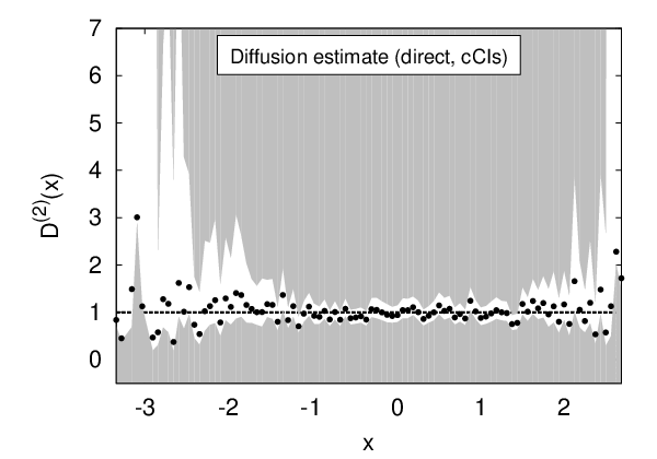

Beyond the calculation of the most likely parameters, likelihood functions also are required for the calculation of BpCIs. Details on how this procedure can be performed for the particular functions (17) are outlined in appendix A, together with remarks on the calculation of the respective cCIs for the direct estimation procedure. Both the maximum likelihood and the direct estimation procedures were applied to one realisation of an Ornstein-Uhlenbeck process with sampled at . The estimation results are depicted in figure 1. For the non-parametric maximum likelihood estimation (two upper rows) two different realisation of BpCIs are shown, one with constant (upper row) and one where the individual were iterated to achieve a constant significance level of (second row). Figure 2 demonstrates the effect of the iteration of on the confidence levels of BpCIs for the diffusion estimate.
Results of the direct estimation procedure for the diffusion
differ slightly from the maximum likelihood estimates
(18). These differences, however, only seem to be
relevant at the sparsely sampled boundaries, where the term
can become large. In the central regions with a
sufficient amount of samples per bin differences in the respective
confidence intervals are relatively small. Here BpCIs correspond very
well to cCIs, a fact already mentioned in section
III. In the sparsely sampled regions cCIs of
generally are larger than the respective BpCIs, which is a
result of the deviation of Student’s t-distribution from
normality. For the diffusion estimates the respective confidence
intervals in the sparse regions differ quite significantly: The BpCIs
with constant significance level are largest and, therefore, probably
most conservative. Comparison between the uppermost and the second row
and inspection of figure 2 suggests
that Wilks’ theorem might not safely be applicable in sparsely sampled
regions. All confidence intervals almost everywhere contain the true
parameter values indicated by the dashed lines.
Generally the differences between the maximum likelihood estimates and
the direct estimation procedure are almost negligible and the
potentially small improvement in the confidence intervals for
in many cases hardly may justify the application of this more complex
estimation procedure. The non-parametric estimation generally suffers
from huge uncertainties in sparsely sampled regions. For this reason a
quantitative interpretation of the estimates often is difficult.
If a quantitative characterisation of the system is required one
possibility is to fit parametrized drift and diffusion functions to
the non-parametric estimates. From inspection of figure
1 we can understand that this procedure might
not be straightforward, since one typically is faced with several
questions: which regions should be fitted? How should one account for
the confidence intervals, in particular for the asymmetric ones for
the diffusion estimate? In particular the latter question is not as
trivial as it seems.
If we for convenience assume that the confidence intervals for
are symmetrical and that they correspond to quantiles of a normal
distribution standard procedures can be used to fit the
parametrizations (13) of drift and diffusion to the
direct estimates for drift and diffusion exhibited in the lower
panels of figure 1. Two least square fits
were performed, one fitting the estimates only (NP-DE) and another
weighting the estimated by the reciprocal squared width of the
respective confidence intervals (NP-DE-CI). The results are compiled
in table 3 and compared to the
results from maximum likelihood estimation of the parameters as
described in the previous section (MLE). The accuracy of the
parameter estimates NP-DE and NP-DE-CI actually is fine, having in
mind that cCIs were not considered for the estimation (NP-DE) or
assumed to be symmetric (NP-DE-CI). Anyway the precision of the
estimates and the respective confidence intervals seems to be
deficient with respect to the estimation of parameters by maximum
likelihood methods.
| Method | Time | ||||||||||
|---|---|---|---|---|---|---|---|---|---|---|---|
| MLE | |||||||||||
| NP-DE | |||||||||||
| NP-DE-CI | |||||||||||
| BIN-MLE | |||||||||||
VI Estimation at small time increment and stepwise constant drift and diffusion: An efficient parametric procedure
The estimation procedure for parametric drift and diffusion as described in section IV yields accurate estimation results and Bayesian posterior confidence regions if measurement data is available at high sampling frequencies. A drawback of this method, however, is that the calculation of the likelihood functions becomes computationally demanding for large data sets or a complex parameter space. This disadvantage can be solved by combining it with the concept of stepwise constant drift and diffusion functions developed in the previous section.
Let us assume that we have partitioned the data into non-overlapping bins, calculated the respective centres of mass , the index sets from (14), the frequencies , and the conditional moments according to (16). For a given combination of drift and diffusion coefficients in the individual bins, , the log-likelihood function then can be calculated as
| (19) |
where the contributions of the individual bins are given by (17). If we have a parametric form of and depending on a set of parameters such as e.g. (13) the coefficients in the individual bins for a particular can be defined as
| (20) |
where the functions are evaluated at the centre of mass of the respective bins. Then, equation (19) can be used for calculation of the log-likelihood of ,
| (21) |
This expression needs to be maximized with respect to . An example for the numerical implementation procedure is included in appendix B (procedure parBinMLE). Results for optimizing the drift and diffusion functions (13) for synthetic data obtained from sampling an Ornstein-Uhlenbeck process are listed in table 3 (case BIN-MLE, last row).
Optimising expression (21) has
advantages with respect to the procedures for parametric estimation
outlined in sections IV and
V: With respect to the optimisation of the
exact small- log-likelihood function,
(5) with propagator
(12), the computationally effort is reduced
drastically, in particular for large data sets. Once pre-calculation
of the conditional moments is completed the effort for evaluating the
log-likelihood does not depend on the dimension of the data set but of
the number of bins only. This is an important improvement, in
particular if the dimension of becomes large
and complex maximization algorithms are applied. The significant gain
in computational efficiency already has an effect at data sets
consisting of points, where the computational effort roughly
is decreased by the order (rightmost column of table
3).
With respect to the procedure outlined in the previous section, i.e. calculation of a non-parametric estimate and fitting the respective
functions, maximizing the log-likelihood yields much more precise
results (table 3). Moreover the
calculation of BpCIs is a consistent procedure, whereas fitting of
with its asymmetric confidence intervals cannot be performed
with many standard tools. Finally maximization of
(20) in contrast to
procedures for the non-parametric estimation is not very sensitive to
the binning, since (21) for bins
of equal size converges to (5) with
propagator (12) in the limit . The estimation results listed in table
3 indicate that the procedure for the
sample data set already is sufficiently accurate with .
VII Conclusions
This work addresses the estimation of drift and diffusion functions from time series data by means of maximum likelihood estimators with a particular focus on the statistical accuracy of results through the calculation of confidence intervals for the estimated parameters. The results are discussed in the light of a procedure for the direct estimation of drift and diffusion function, (2), which extensively has been used in several applications.
From the cases studied here we can conclude that maximum likelihood estimators are superior to the direct estimation procedure if quantitative results are required. However for a long time their application for the estimation of general drift and diffusion functions hardly was possible at reasonable effort, since it intensively involved numerical solutions of the Fokker-Planck equation (sections II and III). Within the scope of this work more efficient methods for the estimation of parametric drift and diffusion functions were developed.
In section IV an approximated log-likelihood function for the estimation from data sampled at high frequencies is introduced, which renders numerical solution of the Fokker-Planck equation unnecessary. Although estimators in this limit already were described earlier [25] their performance, at least to my knowledge, was not investigated systematically. From our investigations we see that the estimator yields good results even at small but finite time lags (table 2). The numerical efficiency drastically can be increased if the data, in addition, is partitioned into bins as described in section VI. The application of this estimator e.g. for fitting drift and diffusion functions by low order polynomials such as (13) is only slightly more complex than the direct estimation procedure. For this reason I would like to recommend this procedure for the quantitative estimation of parametric drift and diffusion functions from data available at sufficiently high sampling frequency.
An advantage of the maximum likelihood approach is, that it is straightforward to define Bayesian posterior confidence intervals (BpCIs) for any parameter estimated. To my knowledge this problem had not been addressed in connection with the estimation of drift and diffusion functions, although of very high relevance for the quantitative discussion of results. The calculation of BpCIs is explained in great detail in section III and demonstrated by the respective examples in sections II to VI.
In section V the non-parametric estimation of
drift and diffusion by maximum-likelihood methods is addressed and
discussed in the context of the direct estimation procedure,
(2). A similar procedure also is investigated in a
recent arXiv preprint by Ohkubo which uses kernel density estimators
for the transition probability density functions [29]. In
contrast we apply a partition of the data into non-overlapping bins,
which is more straightforward to implement and which results in a
simple connection between global and local likelihood functions,
(15), a fact that is essential for the
efficient parametric estimation procedure developed subsequently.
It is shown that the direct estimation slightly differs from
the most likely estimates only in the diffusion term. Interestingly
these differences correspond to finite- correction for the
direct estimation procedure proposed in [16] that
was debated intensively [17, 35].
Results derived in section V and in appendix
A also are relevant for application of the
direct estimation procedure, which until now lacked a detailed
discussion of the statistical errors. It is expected that the
resemblance to the maximum likelihood estimates and the assumption
required for this purpose (i.e. the small- approximation and
the assumption of stepwise constant drift and diffusion functions, see
section V for details) also might ease the
interpretation of direct estimates of drift and diffusion.
A great deal of the methods developed in this work relies on the small- approximation of the propagator, (12), which only is applicable at sufficiently large sampling frequencies. It is difficult to give an exact and general criterion which frequencies are required in each case. As a rule of thumb the sampling, however, needs to allow both for resolving the microscopic fluctuations at small time scales and a sufficiently large fraction of phase space. For cases where the accuracy of the small- approximation is questionable it is recommended to validate the results by methods not explicitly incorporating this approximation as e.g. described in section II and in [19, 31].
At several instances the efficacy of the approximates for the log-likelihood functions and the straightforward implementation of the estimation procedure were emphasized. The computational costs of the different approaches are compared in table 3 and show, that in particular the computational effort for the procedure outlined in section VI is very low, in spite of the optimization of a five-dimensional parameter vector. The Python codes used for benchmarking including the implementation of the respective estimation procedures are listed in appendix B. I hope that these examples give ideas about potential implementations of the estimation procedure and stimulate the application of maximum likelihood estimators and Bayesian posterior confidence intervals for the analysis of relevant measurements.
Acknowledgements
I kindly would like to acknowledge discussions with Rudolf Friedrich, Joachim Peinke, Maria Haase, Christoph Honisch, Bernd Lehle, and Pedro Lind at the Dynamic Days Europe 2011, where this work was presented first. Christoph Honisch furthermore pointed me to reference [29], which covers a topic similar to section V of this work, although from a slightly different perspective. I was glad to be able to include this contribution in the discussion. All numerical simulations and calculations were performed with Python and I thank Frank Raischel for introducing me to this language recently and Philip Rinn for comments on the code. This work was supported by a Linnaeus-grant from the Swedish Research Councils, VR and Formas (http://www.cemeb.science.gu.se).
Appendix
Appendix A Confidence intervals for the non-parametric estimates
This appendix addresses the calculation of Bayesian posterior confidence intervals (BpCIs) for the non-parametric maximum likelihood estimates and classical confidence intervals (cCIs) for the direct estimates, (2). It uses nomenclature and variables as introduced in section V. The respective confidence intervals were used for preparation of figure 1.
For the individual bins BpCIs for drift and diffusion can be calculated by the method introduced in section III. For the drift coefficients the expressions can be evaluated analytically. With help of some algebra it can be shown that the log-likelihood offset calculated from Wilks’ theorem independently of the sample size provides BpCIs exactly at the desired confidence level. For the drift in bin the BpCI at at level is with
| (22) |
where is the inverse of the error function at
the desired confidence level . This interval is consistent with
classical confidence intervals for the mean of samples with known
variance (which is a consequence of the fact that we investigate
estimation errors in and independent from one
another as described in section III). For the
confidence level one obtains
.
As already previously noted for cCIs of direct estimates
[36] the size of BpCIs for the drift estimates
diverges in the limit , which renders the fact that the
estimation problem for the drift is ill-posed
[37]. Throughout this work we, however, could observe, that
estimation at small but finite yields satisfactory results and
that the respective confidence intervals accurately reflected the
statistical uncertainties of the drift estimates relevant at small
time lags.
BpCIs of the diffusion estimates to our knowledge cannot be derived analytically but need to be iterated numerically from equation (10a). For at least a closed expression of the confidence level of the BpCI associated to a certain can be calculated by inserting (17) into (10b),
| (23) |
where is the cumulative distribution function of the distribution at with degrees of freedom. This expression can either be used for verification of the confidence level for a constant or for iteration of (and boundaries of the corresponding confidence interval) until a desired confidence level is reached. For bins with BpCIs for the diffusion estimate cannot be calculated since (10b) diverges.
For the direct estimates, (2), classical confidence intervals (cCIs) at confidence level can be calculated from quantiles of Student’s t and the distribution, respectively. For the drift estimates the confidence intervals are symmetric with respect to the estimated drift coefficients. For bin the cCI at level is with
| (24) |
where is the inverse cumulative distribution function of Student’s t-distribution with degrees of freedom, evaluated at . For the significance level relevant in this manuscript for large sample sizes is obtained, which equals the respective value for the BpCIs for the drift estimates calculated above.
cCIs of the diffusion estimates are asymmetric. The boundaries of the cCIs for the diffusion estimate in bin at level can be calculated as
| (25a) | |||||
| (25b) | |||||
where is the inverse cumulative distribution function of the distribution with degrees of freedom evaluated at . Quantiles of distribution functions such as Student’s t or the distributions in the meanwhile accurately are iterated numerically by standard packages as e.g. applied in the Python codes used for preparation of this manuscript as listed in appendix B.
Appendix B Python code: Implementation of estimation procedures and benchmark
This appendix contains listings of Python code used for preparation of the tables and figures contained in this manuscript. Python is available without charge for most software environments. The codes were tested with version 2.6.5.
The file python_procedures.py contains examples for implementations of the parametric estimation procedures described in sections IV (parMLE) and VI (parBinMLE). In addition an implementation of the direct estimation procedure for the non-parametric estimation is included (nonParDirect), that yields classical confidence intervals for the estimates calculated according to appendix A.
The file python_main.py exhibits an example of how the individual procedures can be used on a specific data set. This code has been used for calculation of the results and benchmarks listed in table 3.
References
References
- [1] H. Haken, Synergetics, Springer Series in Synergetics (Springer-Verlag, Berlin, 2004) ISBN 3-540-40824-X, pp. xvi+763, introduction and advanced topics, Reprint of the third (1983) edition [Synergetics] and the first (1983) edition [Advanced synergetics]
- [2] For reasons of clarity we here restrict to a one dimensional process. Generalisation to higher dimensions, however, is straightforward (see e.g. [38, 3, 39]).
- [3] H. Risken, The Fokker-Planck equation, 2nd ed., Springer Series in Synergetics, Vol. 18 (Springer-Verlag, Berlin, 1989) ISBN 3-540-50498-2, pp. xiv+472, methods of solution and applications
- [4] S. Siegert, R. Friedrich, and J. Peinke, Physics Letters A 243, 275 (1998)
- [5] R. Friedrich, S. Siegert, J. Peinke, S. Lück, M. Siefert, M. Lindemann, J. Raethjen, G. Deuschl, and G. Pfister, Physics Letters A 271, 217 (2000)
- [6] D. Lamouroux and K. Lehnertz, Physics Letters A 373, 3507 (2009)
- [7] R. Friedrich and J. Peinke, Phys. Rev. Lett. 78, 863 (1997)
- [8] S. Lück, J. Peinke, and R. Friedrich, Phys. Rev. Lett. 83, 5495 (1999)
- [9] J. Gottschall and J. Peinke, Journal of Physics: Conference Series 75 (2007)
- [10] R. Friedrich, J. Peinke, and C. Renner, Phys. Rev. Lett 84, 5224 (2000)
- [11] S. Kriso, R. Friedrich, J. Peinke, and P. Wagner, Physics Letters A 299, 287 (2002)
- [12] T. Kuusela, Physical Review E 69, 031916 (2004)
- [13] J. Prusseit and K. Lehnertz, Physical Review Letters 98, 138103 (2007)
- [14] R. Friedrich, J. Peinke, M. Sahimi, and T. M. R. Rahimi, Physics Reports 506, 87 (2011), ISSN 0370-1573
- [15] P. Sura and J. Barsugli, Physics Letters A 305, 304 (2002)
- [16] M. Ragwitz and H. Kantz, Phys. Rev. Lett. 87, 254501 (2001)
- [17] R. Friedrich, C. Renner, M. Siefert, and J. Peinke, Physical Review Letters 89, 149401 (2002)
- [18] J. Gottschall and J. Peinke, New Journal of Physics 10, 083034 (2008), http://stacks.iop.org/1367-2630/10/i=8/a=083034
- [19] D. Kleinhans, R. Friedrich, A. Nawroth, and J. Peinke, Phys Lett A 346, 42 (2005), http://arxiv.org/abs/physics/0502152
- [20] S. J. Lade, Physics Letters A 373, 3705 (2009), ISSN 0375-9601
- [21] C. Honisch and R. Friedrich, Phys. Rev. E 83, 066701 (Jun 2011)
- [22] F. Böttcher, J. Peinke, D. Kleinhans, R. Friedrich, P. G. Lind, and M. Haase, Phys. Rev. Lett. 97, 090603 (2006), http://arxiv.org/abs/nlin/0607002
- [23] P. G. Lind, M. Haase, F. Böttcher, J. Peinke, D. Kleinhans, and R. Friedrich, Physical Review E 81, 13 (2010)
- [24] B. Lehle, Physical Review E 83, 021113 (2011), http://link.aps.org/doi/10.1103/PhysRevE.83.021113
- [25] Y. Ait-Sahalia, Econometrica 70, 223 (2002), http://dx.doi.org/10.1111/1468-0262.00274
- [26] A. W. Lo, Econometric Theory 4, 231 (1988)
- [27] G. Durham and A. Gallant, Journal of Business and Economic Statistics 20, 297 (2002)
- [28] H. Wu and F. Noé, Physical Review E 83, 036705 (2011)
- [29] J. Ohkubo, Preprint available at arXiv.org(2011)
- [30] A. S. Hurn, K. A. Lindsay, and V. L. Martin, Journal of Time Series Analysis 24, 45 (01 2003)
- [31] D. Kleinhans and R. Friedrich, Physics Letters A 368, 194 (2007), http://arxiv.org/abs/physics/0611102
- [32] E. Jaynes, Foundations of Probability Theory, Statistical Inference, and Statistical Theories of Science 2, 175 (1976)
- [33] S. S. Wilks, The Annals of Mathematical Statistics 9, 60 (1938)
- [34] E. Jaynes, Physical review 108, 171 (1957)
- [35] M. Ragwitz and H. Kantz, Physical Review Letters 89, 149402 (2002)
- [36] D. Kleinhans and R. Friedrich, in Wind Energy: Proceedings of the Euromech Colloquium, edited by J. Peinke, P. Schaumann, and S. Barth (Springer Berlin Heidelberg, 2007) pp. 129–133
- [37] Y. Pokern, A. Stuart, and E. Vanden-Eijnden, Multiscale Modeling & Simulation 8, 69 (2009)
- [38] R. Friedrich, J. Peinke, and M. Reza Rahimi Tabar, “Encyclopedia of complexity in science,” (Springer, Heidelberg, Berlin, 2008) Chap. Complexity in the View of Stochastic Processes, (in press)
- [39] C. W. Gardiner, Handbook of stochastic methods for physics, chemistry and the natural sciences, 3rd ed., Springer Series in Synergetics, Vol. 13 (Springer-Verlag, Berlin, 2004) ISBN 3-540-20882-8, pp. xviii+415