On the Effects of Line-of-Sight Structures on Lensing Flux-ratio Anomalies in a CDM Universe
Abstract
The flux-ratio anomalies observed in multiply-lensed quasar images are most plausibly explained as the result of perturbing structures superposed on the underlying smooth matter distribution of the primary lens. The cold dark matter cosmological model predicts that a large number of substructures should survive inside larger halos but, surprisingly, this population alone has been shown to be insufficient to explain the observed distribution of the flux ratios of quasar’s multiple images. Other halos (and their subhalos) projected along the line of sight to the primary lens have been considered as additional sources of perturbation. In this work, we use ray tracing through the Millennium II simulation to investigate the importance of projection effects due to halos and subhalos of mass and extend our analysis to lower masses, , using Monte-Carlo halo distributions. We find that the magnitude of the violation depends strongly on the density profile and concentration of the intervening halos, but clustering plays only a minor role. For a typical lensing geometry (lens at redshift 0.6 and source at redshift 2), background haloes (behind the main lens) are more likely to cause a violation than foreground halos. We conclude that line-of-sight structures can be as important as intrinsic substructures in causing flux-ratio anomalies. The combined effect of perturbing structures within the lens and along the line of sight in the CDM universe results in a cusp-violation probability of 20-30%. This alleviates the discrepancy between models and current data, but a larger observational sample is required for a stronger test of the theory.
Keywords:
gravitational lensing: strong - galaxies: haloes - galaxies: structure - cosmology: theory - dark matter.1 INTRODUCTION
In the cold dark matter (CDM) cosmogony, galaxies are biased tracers of a filamentary “cosmic web” of collapsed regions in the matter density field – dark matter haloes. The excellent agreement between the predictions of this model and observations of the large-scale clustering of galaxies provides compelling support for CDM. However, on the scale of individual dark haloes, the model makes a number of predictions that have yet to be fully verified: cuspy halo density profiles and a large population of surviving dark matter substructures. These substructures are the cores of accreted CDM haloes that persist as long-lived gravitationally bound subhaloes (Gao et al., 2004; Diemand et al., 2008; Springel et al., 2008). Therefore, measurements of halo density profiles and of the subhalo abundance are crucial tests of the cosmological model.
Galaxies and their dark matter haloes can act as strong gravitational lenses, producing distorted and even multiple images of more distant galaxies and quasars. The distribution and properties of these images provide sensitive probes of the mass distribution in the lens. In some multiply-lensed quasar systems, simple parametric mass models can fit image positions well, but not their flux ratios. Such anomalies are interpreted as evidence for complex substructures in lensing galaxies11 1 Apart from quasar images’ flux-ratio anomalies, another promising method is to use surface brightness anomalies of lensed galaxies to identify substructures and constrain their properties, see e.g., Vegetti & Koopmans (2009); Vegetti et al. (2010). (Mao & Schneider, 1998; Metcalf & Madau, 2001; Metcalf & Zhao, 2002; Chiba, 2002; Metcalf et al., 2004; Sugai et al., 2007; McKean et al., 2007; More et al., 2009; MacLeod et al., 2009).
On scales probed by galactic strong lensing (typically a few kiloparsecs), predictions from CDM simulations have been compared with observed flux-ratio anomalies (e.g. Dalal & Kochanek 2002; Bradač et al. 2004; Metcalf & Amara 2012). Several studies have concluded that the predicted abundance of dark matter substructures in the strong-lensing regions of galaxy-sized haloes is not sufficient to explain the statistics of the currently available sample of known anomalous lenses (Mao et al., 2004; Amara et al., 2006; Macciò & Miranda, 2006; Chen et al., 2011).
In any smooth lens potential producing multiple images of a single source, a specific magnification ratio (here equivalent to a flux ratio) of the three most strongly-magnified images will approach zero asymptotically as the source approaches a cusp of the tangential caustic. This is known as the “cusp-caustic relation” (see Eq. 3 below) (Blandford & Narayan 1986; Schneider & Weiss 1992; Zakharov 1995; Keeton et al. 2003). Structures, either within a lensing galaxy or projected by chance along the line of sight, will perturb the potential and alter the flux of one or more images, resulting in a violation of the cusp-caustic relation. These violations are extreme cases of flux-ratio anomalies.
Xu et al. (2009); Xu et al. (2010) analyzed flux-ratio distributions of multiple-imaged background quasars in simulated lensing systems, using six CDM haloes and their substructure populations (subhaloes and streams) from the Aquarius project (Springel et al. 2008). The effects of baryonic substructures (satellite galaxies and globular clusters) were also investigated. These exceptionally high resolution simulations confirmed that the substructure abundance (in the critical region of a Milky Way-mass lens) predicted by the CDM model is too low to explain the observed frequency of cusp-caustic violations.
This apparent deficiency of substructures is not yet a strong challenge to CDM, in part because the sample of observed lenses is extremely small. Furthermore, dark matter haloes and subhaloes are present along the entire line of sight from the source to the observer, not just in the lens itself. These independent haloes projected in front of and behind the lens can also induce perturbations to the lensing potential and thus cause flux-ratio anomalies (Chen et al., 2003; Wambsganss et al., 2005; Metcalf, 2005a; Metcalf, 2005b; Miranda & Macciò, 2007; Puchwein & Hilbert, 2009).
In particular, Chen
et al. (2003) used the cross-section (optical depth)
method to calculate the effect of both subhaloes intrinsic to the main
lens and line-of-sight haloes. They found that the former would
dominate the total lensing cross-section, although the exact
percentage was highly sensitive to the spatial distribution of
substructures22
2
A similar conclusion was reached by
Xu
et al. (2009); Xu et al. (2010); see also Nierenberg et al. (2011) for
the observed spatial distribution of luminous satellites in
early-type galaxies.; the latter – line-of-sight haloes, modelled
as singular isothermal spheres – would contribute to
of the total perturbation. Metcalf (2005a) performed ray-tracing
simulations for the line-of-sight lens population () in a CDM universe,
which he compared to several observed systems with measured
cusp-caustic ratios. Assuming that haloes have Navarro, Frenk & White
(NFW) profiles (Navarro
et al. 1996; Navarro
et al. 1997), Metcalf found that the
predicted abundance of line-of-sight haloes was enough to explain the
observed flux-ratio anomalies of several representative cases. With a
slightly different approach and assuming haloes to be singular
isothermal spheres, Miranda &
Macciò (2007) found that, with the
additional contribution from haloes along the line of sight, the
observed flux-ratio anomalies can be reproduced with a high
confidence level.
In this work, we re-examine the perturbing effect of haloes along the entire line of sight from the source to the observer by using -body simulations to generate strong-lensing sight lines and quantify the flux-ratio distributions for multiply-imaged sources. In 2, we introduce our method for tracing light deflection through multiple lens planes. In 3, we present a summary of the cusp-caustic violations arising from simple perturbation scenarios (varying the density profiles, angular positions and redshifts of the perturbers). In 4, we describe our method for generating “lensing lighcones” in the Millennium II CDM -body simulation (Boylan-Kolchin et al. 2009). Results from the analysis of these lensing cones are given in 5. In 6 we present results using a Monte-Carlo approach to account for haloes below the mass resolution limit of Millennium II (). Our conclusions are given in 7. The cosmology of our lensing simulations is the same as that used for the Millennium-II simulation, with a matter density , cosmological constant , Hubble constant and linear fluctuation amplitude . These values are consistent with cosmological constraints from the WMAP 1- and 5-year data analyses (Spergel et al. 2003; Komatsu et al. 2009), but differ at about the 2 level from more recent WMAP 7-year determinations (Komatsu et al. 2011). This small offset is of no consequence for the topics addressed in this paper.
2 Simulations of Light Deflection through Multiple Lens Planes
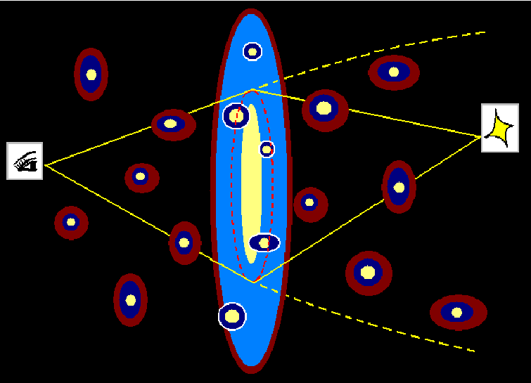

In Chapter 9 of Schneider et al. (1992), the authors present the theory of light deflection through multiple lens planes. As shown in Fig. 1, haloes are projected near the line of sight at all redshifts between the observer and a source at redshift . The angular position of the source is denoted by , and its final image position is denoted by . The haloes are assumed to be distributed in lens planes, each at redshift (=1,2…, and ). As the light ray passes through each plane, the image position (where the light ray intercepts the plane) in the ()-th lens plane, which is also the source position for the -th plane, is related to and by the lens equation:
| (1) |
where , and . is the deflection angle a light ray undergoes in the -th plane at . and are angular diameter distances between the ()-th plane and the observer, and between the ()-th plane and the -th plane, respectively. is the angular diameter distance of the source. The Jacobian matrix of the mapping between and the source position for the -th plane is given by:
| (2) |
and is the overall Jacobian matrix, describing the mapping relation between and .
Images of any given background source can be accurately and efficiently identified using the Newton-Raphson method, once the mapping relation (the overall Jacobian matrix ) is obtained. We determine the Jacobian matrix numerically, as follows. For each lens plane, a rigid grid of is applied to cover a central region of . Source positions that correspond to grid points in the first lens plane (which is also the final image plane) are calculated through the multi-plane lens equation (Eq. 1). An arbitrary light ray propagating through a lens plane will not necessarily hit a grid point of the mesh that covers that plane. Therefore, for any given position of the -th lens plane, the deflection angle is obtained by linear interpolation using the values for the four nearest grid points. Once is obtained, the Jacobian matrix for the image plane grid points can be derived using finite differencing with the five-point stencil method (accurate to the third order). Again, linear interpolation is used to obtain each element of the Jacobian matrix, , at any given image position . The corresponding image magnification is then given by .
We use our multi-plane ray tracing code with a resolution of 0.005 per pixel in the lens and image planes, which we find sufficient to accurately reproduce the lensing properties of a number of simple analytical cases.
3 Anomalous Flux Ratios and Cusp-Caustic Violations

The cusp-caustic relation (Blandford & Narayan 1986; Schneider & Weiss 1992; Zakharov 1995; Keeton et al. 2003) is defined as:
| (3) |
when . denote the magnifications of the three closest images (, and ) of a background point source located near a cusp of the tangential caustic (as shown in Fig. 2). Observationally, source positions cannot be directly measured – instead, an image opening angle is often used as an indicator of the proximity of a source to the nearest cusp of the tangential caustic. This opening angle is measured between lines joining the centre of the lens to the two outer images and . As the source moves outwards (towards the nearest cusp), , , and will go to zero asymptotically. This relationship holds for any smooth lens potential.
Fig. 2 illustrates how perturbing structures change the cusp-caustic relation. The upper panels show the critical curves in the image plane, and the bottom panels are contour maps of for sources within the tangential caustic in the source plane. Left and right columns show smooth lens potentials and lens potentials with substructures, respectively. Substructures located near the critical curve will affect images nearby and result in significantly larger values of , violating the predicted ratios of image magnifications (fluxes) given by Eq. (3).
3.1 Observational samples
Multiple images of lensed quasars with small are ideal cases to examine violations of the cusp-caustic relation and can be used to put constraints on the properties of perturbing structures. This is especially true when their fluxes are measured in the radio and mid-infrared, as the interpretation of optical and near-infrared flux ratios is complicated by stellar microlensing and dust extinction. At the present time, only five cusp-geometry lensing systems with image opening angle are known. These were used for statistical comparisons to the simulations in our previous work (Xu et al. 2009; Xu et al. 2010). All five cases have surprisingly large values which are difficult to explain with simple smooth lens models. Of these five (flux-ratio measurements), two that were obtained in the optical have been proven to be affected by microlensing; the other three were from the CLASS survey (Browne et al. 2003; Myers et al. 2003) at radio wavelengths and are thought to be more secure cases of perturbations due to substructures in the lens.
| Systems | Reference | ||
|---|---|---|---|
| (1) B2045+265 | 34.9 | 0.501 | Fassnacht et al. (1999) |
| Koopmans et al. (2003) | |||
| (2) B0712+472 | 76.9 | 0.255 | Jackson et al. (1998) |
| Koopmans et al. (2003) | |||
| (3) B1422+231 | 77.0 | 0.187 | Patnaik et al. (1999) |
| Koopmans et al. (2003) | |||
| (4) MG0414+053 | 101.5 | 0.227 | Hewitt et al. (1992) |
| Katz et al. (1997) | |||
| (5) B1555+375 | 102.6 | 0.417 | Marlow et al. (1999) |
| Koopmans et al. (2003) |
Table 2 of Chen et al. (2011) lists all of the currently observed - pairs for systems with four distinct point-like images of quasars lensed by one single galaxy. Our Table 1 lists those with their flux ratios measured in the radio and image opening angles . We compare our simulations with this observational sample of lenses, with no additional selection criteria.
Notice that four of the five lenses listed in Table 1, namely, B0712+472, B1422+231, B2045+265 and MG0414+053, are reported as having visible companions (satellites/group galaxies) projected near the main lensing galaxies (Fassnacht & Lubin 2002; Hogg & Blandford 1994; Grant et al. 2004; McKean et al. 2007; Falco et al. 1997). Fitting the observed image positions using a singular isothermal ellipsoidal model yields velocity dispersions ranging from km/s, and axis ratios between (Sluse et al. 2011), except for B1555, which requires km/s and (Marlow et al. 1999).
3.2 Statistical measures for the cusp-caustic violation: and
Given a simulated lensing system, we compare to the observations in Table 1 by generating a large number of realisations of background sources with . We calculate for each realisation and evaluate for this ensemble of realisations. This is defined as the probability for , measured for sources with image opening angles (i.e. within a five-degree opening-angle span centred at ) to be larger than a particular threshold value. Lenses with more perturbations will result in large values for many source positions and thus have a higher than lenses with fewer perturbations.


We illustrate our use of the in Fig. 3. The top panel shows a
typical example of a close triple image configuration for cusp sources
with . In this case, the lensing
galaxy has a (smooth) singular isothermal ellipsoidal (SIE) profile
(see Keeton &
Kochanek (1998) for notations of , ,
, and herebelow) with lensing strength and
axis ratio , and is located at redshift ; the source
redshift is . The corresponding contour map of in the -
plane is given in the middle panel. Also plotted are the radio
measurements for the currently best available sample (listed in
Table 1). These are clearly
inconsistent with the smooth-lens distribution.
When we include the substructures within the lensing galaxy and its dark matter halo, the regular distribution for a smooth lens potential disappears. The bottom panel in Fig. 3 shows the average distribution of when including the subhalo population from the Aquarius simulations (Xu et al. 2009). At small , violations are more significant than on larger scales. The smallest measured among all observed cusp-caustic systems is 0.187 (from B1422). In Xu et al. (2009), we calculated , which is the probability for to be larger than or equal to 0.187, computed over all realizations with . was found to be 10%. We concluded that it is difficult to explain the observed distribution (especially at larger ) with a subhalo population similar to that produced in the Aquarius simulations. This motivates the search for other sources of perturbations to the lens potential.
In this work, we use as an overall estimate for the probability of observing cusp-caustic violations, in order to compare with our previous work. The value of is chosen in order to compare with Amara et al. (2006), who adopted to select cusp-like lenses which can be best used to test the cusp-caustic violation. Varying the upper limit of will change the probability of cases with . However, our final conclusion (in 7) is based on a statistical argument that only applies to the observed lenses with .
3.3 Simple perturbation scenarios with different halo redshifts, masses, profiles and concentrations
A number of parameters determine the importance of these perturbers for creating violations to the cusp-caustic relation: most significant are their masses, density profiles, redshifts and impact parameters to the line of sight. Before presenting the results from general lines of sight taken from -body simulations, we first show several simple perturbation scenarios to illustrate, individually, the effects of these different parameters, in the case of a single perturbing halo.
Fig. 4 shows critical curves and caustics produced by a main-lens potential of an isothermal ellipsoid with , and core size , located at for a source at redshift , plus a perturber of modelled with a truncated singular isothermal sphere. The panels in this figure correspond to different scenarios. In the upper row the perturber’s angular position is fixed (outside the tangential critical curve), and we vary its redshift: (foreground), (in the main-lens plane) and (background). In the lower row, we fix the redshift of the perturber to the main lens plane () and change its impact parameter, such that it is projected within, on top of and outside the tangential critical curve (left to right panels, respectively). Wiggles and swallow tails are introduced to the critical lines and caustics by the added perturbing structure; massive perturbers (or those with compact density profiles) can even cause a secondary set of criticals and caustics. Images located around these wiggle features violate the cusp-caustic relation most strongly.
Fig. 5 shows the contour maps of in the - plane for the different scenarios above. Violation patterns as a function of image opening angle vary with the positions and redshifts of the perturbers. Notice that at redshifts greater than that of the primary lens, the cone of light rays starts decreasing in size towards the source. This means a “background” perturber that appears to be projected close to the critical curve (where images normally form) could actually be far away from the light ray. Such perturbers would be less effective in causing convergence fluctuations than their foreground counterparts (they would still contribute to the shear field). However, depending on the distribution of the primary lens and the source, there could be many more background structures affecting the light ray than those in the foreground (see 5).


.


The mass and density profile of a perturber also affect the production of flux-ratio anomalies (and cusp-caustic violations) by altering the effective cross-section. Singular isothermal spheres have been found to be a good approximation for the inner density profiles of relatively massive haloes (Rusin et al. 2003; Treu & Koopmans 2004; Rusin & Kochanek 2005; Koopmans et al. 2006), where baryons are thought to dominate their central potentials. This effect may be less important in smaller haloes, where the density profile is more likely to be well approximated by the NFW distribution characteristic of CDM haloes in -body simulations (Navarro et al. 1997). Nevertheless, there is still much controversy whether observed low-mass haloes around dwarf galaxies have core-like shallow profiles (Oh et al. 2011).
In the simple scenarios presented below and in our line-of-sight lensing simulations (see 5 and 6), we model perturbing haloes either as truncated singular isothermal spheres33 3 A singular isothermal sphere may not be a realistic model for small haloes. We adopt this model for ease of comparison with previous work, e.g. Chen et al. (2003). or truncated NFW profiles, normalized with their masses and truncated at their virial radii. We follow the convention of defining the virial radius as , the radius within which the mean halo density is 200 times the critical density of the Universe (at the appropriate redshift ). The mass enclosed within is denoted as . For the NFW profile, the concentration parameter is , where is the scale radius. This parameter is thought to correlate with mass and redshift . A number of concentration-mass relations have been proposed in the literature, based on -body simulations.
In this work, we adopt the concentration-mass relation of Macciò et al. (2008) (hereafter M08) wherever we model perturbers as truncated NFW profiles. The fitting formula (for a WMAP-1 cosmology, close to that of the Millennium-II simulation) is given by:
| (4) |
where .
The concentration-mass relation of Bullock et al. (2001) was used by Metcalf (2005a); Metcalf (2005b) to study how line-of-sight haloes () contribute to the flux anomaly problem. The adopted fitting formula was given by (Metcalf 2005b):
| (5) |
To compare with Metcalf (2005a); Metcalf (2005b), we also perform our analysis using this alternative concentration-mass relation, hereafter referred to as B01-M05.
Fig. 6 shows how these different assumptions for the mass, density profile and concentration-mass relation of a perturber change the total critical curves produced by a primary lens at and the perturbing halo located at the same redshift and with a mass of . A different density profile (a truncated singular isothermal sphere, a truncated NFW profile with the M08 concentration-mass relation and a truncated NFW profile with the B01-M05 concentration-mass relation) is assumed in each row of Fig. 6. Different distortions to the critical curve correspond to different levels of violations in the smooth-lens flux-ratio relationship.
The mass dependence of the violation pattern has been studied systematically, with results presented in 6, which also includes a discussion of effects from different concentration-mass relations and from allowing scatter in the concentration on the overall cusp-violation probabilities.
In this section we have illustrated the effects of varying the redshift, impact parameter, mass and density profile of a single perturbing halo. In practice, perturbations could arise anywhere along the line of sight and from many different haloes. The overall perturbation is far more complicated than any of the simple cases presented here. In the following sections, we use cosmological -body simulations to obtain self-consistent and realistic distributions of perturbers along strong lensing sight lines, and estimate the net perturbation and the likelihood of the observed flux ratio violations.
4 Lensing Lines of Sight from Cosmological Simulations
4.1 Constructing lensing cones from MS-II
The Millennium-II simulation (MS-II; Boylan-Kolchin et al. 2009) is an -body simulation of a cubic cosmological volume with a comoving side length of 100, at a spatial resolution of 1 and mass resolution of . The cosmological parameters of MS-II are the same as those of the earlier Millennium and Aquarius simulations, consistent with the WMAP-1 results. MS-II provides us with the large-scale distributions of a cosmological sample of dark matter haloes. When tracing lensing sight lines through this simulation, we use the following method to determine where haloes cross the past light cone of a fiducial observer (for more details, see Angulo 2008).

We start by replicating the 100 Mpc simulation box in its , and dimensions, as many times as we need to cover the desired redshift range (along the sight line) and angular size (transverse to the sight line). For computational efficiency we only let the combined box go to the source redshift in the and dimensions, and keep the number of replications in the dimension to a minimum. As illustrated in Fig. 7, the observer is located at the origin (0, 0, 0) in one corner of this replicated box. Assuming a source redshift of , the total dimension of the combined box is chosen to be , in units of one Millennium-II simulation box. The position angles of a given line-of-sight vector are defined as the angles measured from the - and -plane, respectively. The simulated sky into which we trace sight lines is then two stripes, which cover and , and . Directions along the and axes (with ) and along have been excluded to avoid significant repetition of structures in the replicated box.
Haloes at each simulation snapshot (corresponding to a particular
redshift) are identified using the Friends-of-Friends algorithm
(Davis et al. 1985). Haloes also contain many subhaloes; these
are identified using the subfind algorithm
(Springel 2005). The minimum mass of subhaloes resolved by
the simulation is (corresponding to 20
particles). Haloes at different snapshots are linked together by an
algorithm for defining their merging history (Helly et al. 2003). We
follow haloes in each of these merger trees and predict their
trajectories (in the replicated box) between every two adjacent
snapshots. In this way, we can find the exact redshift and comoving
position of a halo at the moment it crosses the past light cone of the
observer. When a halo crosses the light cone, all its subhaloes are
assumed to cross at the same redshift. We assume that the relative
positions of these subhaloes at the light-cone crossing time are the
same as in the previous snapshot.
Hereafter, we will use the term “lensing cone” to refer to the observer’s light cone that encloses a particular lensing sight line towards a certain direction in the sky (and out to the source redshift). All haloes that cross the past light cone are checked to see if they are physically within a given lensing cone. If so, their positions, redshifts, masses and half mass radii are stored for lens modelling. All lensing cones are -wide, out to a source redshift , and contain a primary lens around redshift (typical source and lens redshifts for the observed quasar lensing systems).
To build up our lensing cone catalogue, we randomly select about 300 directions in the simulated sky, each of which goes through at least one galaxy-scale halo with a mass above located at redshift in the replicated box. This ensures that the primary haloes we select are responsible for producing multiple images of the background sources. We have confirmed that these 300 randomly selected primary lenses are representative of mass and circular velocity distributions of 23,000 haloes that meet the same selection criteria in the simulated sky.
As stated in §4.2, velocity dispersions of the simulated main lensing haloes range from 200 to 300, comparable to our sample of observed lenses (see the end of §3.1). As the selection function of the observed lenses is hard to define, we assume that they are a random sample of haloes in the ranges of velocity dispersion and redshift given above. Furthermore, by imposing a lower mass limit of on the main lens, we have excluded cases where two or more less massive haloes aligned along the same line of sight produce a comparable strong-lensing signal. However, the chance is small for two foreground haloes, both more massive than , to be well aligned to jointly lens a background galaxy. Emprically, such “three-dimensional” lenses are rare: in the CLASS survey, only one probable such case has been reported out of a total of 22 candidates (Chae et al. 2001; Augusto et al. 2001).

Fig. 8 shows the geometry and halo distribution of an example lensing cone. All haloes within a given cone are used for the lensing calculation. On average each lensing cone (of ) contains about () haloes (subhaloes). Within a projected central region of for strong lensing, there are on average haloes with directly contributing to the convergence field. The rest are distributed further out (in projection) and contribute to the shear field of this region in the same way as point masses.
4.2 Ray-tracing through MS-II lensing cones and line-of-sight lens modelling
To carry out calculations for multi-plane light deflection, we assume 60 lens planes distributed with equal spacing in redshift between the observer and the source at . In each of these lens planes, a region of around the line centre is covered by a rigid grid in order to calculate the Jacobian matrix (Eq. 2) between the source plane and the final image plane.
Haloes within a lensing cone are projected into these lens planes according to their redshifts. The main lens halo is modelled as an isothermal ellipsoid, for which a universal axis ratio () and core radius () are assumed. The orientation of the ellipsoid is randomly chosen in the interval of [0, 2]. The lensing strength (related with through , where , see Keeton & Kochanek 1998) is derived through an empirical relationship between halo’s virial velocity and the velocity dispersion of the equivalent isothermal ellipsoid (Chae et al. 2006):
| (6) |
and , where is the speed of light and and are the angular diameter distances between the main lens and the source, and the source and the observer, respectively. The virial velocity is obtained from halo mass and its virial radius through . Our requirement that the main lens be more massive than results in ranging from 200 to 300, with a weighted mean (by cross-section, ) of 222 corresponding to a lensing strength of for our adopted lens and source redshifts ().
Within each lensing cone, haloes with projected profiles that are completely outside the central region are treated as point masses. Those within this region are assigned a density profile: as described above, we investigate three distinct choices of this profile (singular isothermal sphere, NFW with the M08 concentration-mass relation, and NFW with the B01-M05 concentration-mass relation). All halo profiles are normalized to their masses and truncated at the virial radii ; subhaloes are truncated at two times their half mass radii.
For each line of sight, deflection angles are individually calculated for the equivalent isothermal ellipsoid of the main lens and for all line-of-sight (sub)haloes, and are tabulated to the meshes at different lens planes. Through ray tracing, source positions that correspond to the final image plane are identified, and the final Jacobian matrix is then derived using the finite differencing method. Images of a given source position are effectively found using the Newton-Raphson iteration method.
5 Results from the Millennium II Simulation
In order to calculate – the probability distribution in the plane for individual lensing cones, we generate cusp sources whose close triple images have image opening angles . We have also calculated for cases with as an overall estimate for cusp-caustic violations to compare with our previous work, in which only cases with were examined for violations (caused by intrinsic substructures within the main lens).
To derive average violation probabilities over all sight lines, we weight and of each lensing cone by the quadruple-image lensing cross-section in the source plane (simply the fractional area within the tangential caustic). We do not account for magnification bias among the cusp sources.
| line-of-sight perturbers | truncated singular isothermal sphere | truncated NFW (M08) | truncated NFW (B01-M05) |
|---|---|---|---|
| haloes + subhaloes | 7.8% | 7.3% | 12.8% |
| haloes only | 7.0% | 5.2% | 9.7% |
| background haloes | 5.0% | 3.2% | 5.8% |
| foreground haloes | 2.0% | 1.9% | 4.0% |
Note: was derived using only substructure populations () from the Aquarius simulations (Xu et al. 2009; Xu et al. 2010). Cases here are using line-of-sight structures (haloes and subhaloes) from the Millennium II simulation (); subhaloes from the main lensing halo have been excluded.


Fig. 9 (upper panels) and Table 2 show that if perturbing structures are haloes (and subhaloes) distributed outside the main lens along the line of sight as in the Millennium-II simulation, where such haloes are resolved to , they cause a non-negligible amount of cusp violations, comparable to those due to the substructures in the lens itself. However, the violation pattern (as a function of ) depends strongly on the density profiles applied to haloes projected near the centre of the line of sight.
5.1 Effects from massive line-of-sight haloes


We have also investigated the effect from line-of-sight haloes more massive than , which are most likely to retain a significant fraction of baryons in their dark matter potential wells. The chance of finding at least one of these massive secondary lenses intercepting a strong-lensing sight line (i.e. projected within a typical Einstein radius of 1 around the line centre, out to a redshift of 2) is about 10%. Depending on their density profiles, compact haloes (e.g. singular isothermal spheres) could generate severe astrometry anomalies with a probability of a few percent, while haloes with shallower inner profiles could not.
Fig. 10 presents the peculiar image configurations for an example sight line. Four, six and eight images (excluding the central image) are produced when the source is located at different positions with respect to two sets of tangential caustics. In this particular case, the second caustic is produced by a perturbing halo of , modelled as a truncated singular isothermal sphere, projected near the centre of the main lens. Such peculiar image astrometry has already been proposed and used to constrain density profiles of massive intergalactic objects (e.g., Wyithe et al. 2001; Wilkinson et al. 2001).
5.2 Substructures inside line-of-sight haloes
To investigate the effect of substructures inside haloes along the line of sight, we have excluded all substructures from our Millennium-II lensing cones and calculated violations due to “smooth” line-of-sight haloes alone. Table 2 lists violation probabilities in this case (for different halo density profiles). The relevance of subhaloes to lensing flux-ratio anomalies strongly depends on their assumed density profiles. Comparison of the first and second rows of Table 2 shows that for , NFW-like substructures within line-of-sight haloes are responsible for causing a few percent of the cusp-caustic violations.
5.3 Background vs. foreground
We have separated line-of-sight haloes that are distributed in front of and behind the main-lens plane (). The violation probabilities of these two groups are listed in Table 2, calculated excluding their subhaloes. A higher violation probability is found caused by haloes in the background than in the foreground, as more haloes intercept the light rays behind the main lens plane, given a typical lensing geometry ( and ). It is interesting to notice that violations from the foreground and the background roughly add up to the total violations due to haloes along the entire line of sight (second row of Table 2). The ratio between violations from the foreground and from the entire sight line is close to 2:5, which is the ratio between the comoving radial distances for and .
6 Results from Monte-Carlo haloes with a Sheth-Tormen mass function
The Millennium-II simulation has a limited mass resolution. To investigate the mass dependence of the violation pattern below the halo mass of , we have used a Monte-Carlo method to generate intergalactic halo populations with masses (see 7 for discussion on adopting as the lower mass limit). These haloes are drawn from the Sheth-Tormen mass function (Sheth & Tormen 2002) generated with the code provided by Reed et al. (2007).
We have randomly generated 200 lensing cones out to , each of which contains a main lensing halo modelled as an isothermal ellipsoid at redshift . The lensing strength is fixed to be , the same as the mean of the main lenses in the selected sample of the Millennium-II lensing cones. The axis ratio , core radius and an orientation angle of 0.25 are also taken to be the same for all main lenses.
| () | ||||
|---|---|---|---|---|
| 414 | 50 | 6 | 0.7 | 0.1 (/arcsec2) |
In each realization of the lensing cone, line-of-sight halo positions are randomly generated, with number densities as given by the Sheth-Tormen mass function at the redshifts of the 60 lens planes used for the Millennium-II lensing cones. Table 3 lists the mean surface number densities of projected haloes in different mass decades, averaged over 200 lensing cones44 4 These numbers roughly follow a power-law mass function of , being the mass of haloes.. Haloes projected within the -cone are saved, and those projected within the central -region are modelled with truncated singular isothermal spheres and truncated NFW profiles (using both M08 and B01-M05 concentration-mass relations). Those further out are modelled with point masses. Cusp-caustic violations were identified in the same way as for the Millennium-II lensing cones.
6.1 Mass dependence of the cusp-caustic violation
| truncated singular isothermal sphere | 8.2% | 7.7% | 6.5% | 4.8% | 2.8% |
| truncated NFW profile (M08) | 12% | 9.1% | 5.6% | 2.5% | |
| truncated NFW profile (B01-M05) | 23% | 18% | 11% | 5.5% | 1.9% |
The lower panels of Fig. 9 show contour maps using Monte-Carlo realizations of the line-of-sight halo population, with a lower mass limit of . As in the MS-II lensing case, the frequency of cusp-caustic violations depends strongly on the assumed halo density profiles. Table 4 also presents the values of when this lower mass limit is increased, so that the mass dependence of the cusp-caustic violations can be seen.
Applying truncated singular isothermal spheres yields relatively larger contributions to cusp violations from more massive haloes55 5 Xu et al. (2009) estimated the total lensing cross-section for singular isothermal lenses. In this case , and is a positive value, hence the total lensing cross-section will be biased towards massive haloes. (). When truncated NFW profiles are assumed, lower mass haloes would also cause a significant amount of violations. As can be seen from Table 4, when the lower mass limit of line-of-sight haloes decreases from to (), the corresponding violation probabilities, , increase by 2% (1%), 6% (4%) and 12% (7%) when assuming truncated singular isothermal spheres and truncated NFW profiles with the M08 and the B01-M05 concentration-mass relations, respectively.
Comparing Table 4 with Table 2, it can be seen that our Monte-Carlo results are similar to those obtained using the Millennium-II lensing cones in the mass range above . This suggests that the clustering of haloes is not a dominant effect in the production of flux-ratio anomalies for galactic-scale lenses.
6.2 Dependence on the Einstein radius
| truncated singular isothermal sphere | 6.4% | 8.2% | 11% | 15% |
| truncated NFW profile (M08) | 9.5% | 12% | 15% | 20% |
| truncated NFW profile (B01-M05) | 20% | 23% | 28% | 32% |
When the lower mass cutoff for main lensing haloes in the Millennium-II lensing cones is reduced from to , the mean lensing strength of the equivalent isothermal ellipsoids decreases from to (corresponding to for and using Eq.6). Table 5 presents the values that result from four different for the main lenses in our Monte-Carlo lensing cones. In addition to and , we have calculated violations for an arbitrary of (), which is about the mean (largest) Einstein radius of the observed systems listed in Table 1.
As can be seen clearly from Table 5, systems with larger Einstein radii have higher violation probabilities. This is expected, because close triple images normally form around the tangential critical curve at about the Einstein radius. Comparing to the case of a small Einstein radius, a larger value of this radius results in a higher chance for the image triple (of a given opening angle ) to be intercepted by line-of-sight perturbers.
6.3 Halo concentrations and mass function

As we have shown above, the cusp-violation probability depends strongly on our assumptions about halo concentration. The concentration-mass relation derived by Bullock et al. (2001) has a simple functional form (including redshift evolution) and has been widely used in the literature. Colín et al. (2004) investigated concentration parameters for haloes of and found this relationship to be a good fit. However, these early simulations of dark matter halo formation had relatively low numerical resolution and this can introduce systematic errors.
More recently, a number of authors including Neto et al. (2007), Gao et al. (2008), Zhao et al. (2009) and M08 (whose results are used above), derived concentration-mass relations from high-resolution cosmological -body simulations. These studies are restricted to haloes with but they exhibit systematic differences from the concentrations obtained by B01-M05. For this reason we show lensing results using the M08 relation, extrapolating to lower masses when required, but exploring how the results change when this relation is varied by factors of a few.
The B01-M05 concentration-mass relation overestimates the concentration of small mass haloes inferred from the extrapolated M08 relation by factors of at . Therefore, we expect the violation probability to be larger for the B01-M05 relation than for the M08 relation. The scatter in halo concentration also affects the final cusp-violation probability.
Fig. 11 presents the values of induced by line-of-sight haloes assuming the Sheth-Tormen mass function. To allow for possible uncertainties in halo concentration, we also show results for the case when the concentrations inferred from the M08 concentration-mass relation are multiplied by factors of 0.5, 1.0. 2.0 and 3.0. Varying amounts of scatter in concentration (for haloes of a given mass) are modelled assuming a Gaussian distribution with mean value equal to the M08 concentrations. As may be seen, the violation probabilities depend strongly on halo concentrations. Higher concentrations result in higher cusp-caustic violation probabilities. A larger scatter in concentration will also increase the violation probability.
The halo mass function (the number density of haloes per unit volume per decade in mass) influences the cusp violation probability. Metcalf (2005b) found that flux-ratio anomalies caused by line-of-sight perturbers not only depend strongly on the radial density profile of the haloes (their concentration), but also on the primordial matter power spectrum on small scales. Miranda & Macciò (2007) suggested that flux-ratio anomalies could be used statistically as a test of the behaviour of the matter power spectrum on small scales. We do not explore these effects here but in Fig. 11 we show the result of using the Sheth-Tormen mass function, and assuming that violations grow linearly with the number of perturbers.
7 DISCUSSION AND CONCLUSIONS
We have examined the effects of intergalactic cold dark matter haloes on flux-ratio anomalies in multiply-lensed quasar images by ray-tracing along strong-lensing sight lines that are either taken from the Millennium II simulation (for haloes and subhaloes with ), or generated using the Monte-Carlo method assuming a Sheth-Tormen mass function (for haloes with ).
We use , the probability for the cusp-caustic relation, , to be larger than or equal to 0.187 – the smallest value of measured for cusp-caustic systems to date (for the quasar B1422) – over all realizations with , as a statistical measure of the cusp-caustic violation probability. We have found that the mean violation probability from intervening haloes depends strongly on their density profiles.
Chen et al. (2003) assumed singular isothermal spheres for line-of-sight haloes and find that they only contribute to of the total perturbation. Assuming the same halo density profile, we find that the cusp-caustic violation probability caused by line-of-sight haloes with is comparable to that caused by intrinsic substructures within the main lensing halo ( vs. , Xu et al. 2010), which is in good agreement with Miranda & Macciò (2007). The different results between Chen et al. (2003) and ours can be attributed to the drawbacks of their cross-section method, which underestimates effects from more sophisticated perturbation scenarios (see Metcalf 2005a).
When we assume truncated NFW profiles for the line-of-sight haloes (), the violation probability, , increases to if we adopt the B01-M05 concentration-mass relation and to if we adopt our preferred relation, that by M08. These values are larger than that due to the intrinsic subhalo populations alone.
A typical NFW profile has an Einstein radius orders of magnitude smaller than a singular isothermal sphere with a same mass. However, NFW perturbers in the mass range from to cause more cusp violations than their singular isothermal counterparts. This may be due to the fact that in this mass range, perturbation in magnification (ratios) is mainly from fluctuations in the local density field that do not change the image positions. When comparing an NFW with a singular isothermal sphere of the same mass, we notice that the surface density distribution of the former exceeds that of the latter from a radius of outwards, which means the NFW profile is more effective in introducing fluctuation to the convergence and thus causing flux-ratio anomalies.
On the other hand, the deflection angle of a perturber of is always small ( for
a singular isothermal sphere locating at ), until the perturber
is massive () and compact enough (a
singular isothermal sphere) to have a deflection angle () that can shift a nearby image to a new position with a
different magnification from the primary lens (see
Metcalf 2005b). This can explain the larger violation
probabilities (as shown in Table 4), caused by singular isothermal
perturbers of than by their
NFW counterparts which are less effective in causing flux-anomalies
due to shifting image positions.
Another issue concerns the finite-source effect. Metcalf & Amara (2012) pointed out that biased results about substructures could be drawn due to the point source approximation, which is used in this work.
The radio-emission regions of observed quasars are estimated to be
10 parsecs in extent (Andreani et al. 1999; Wyithe
et al. 2002),
corresponding to for a source at . When
the perturbing mass drops down below , the
corresponding effective perturbing area decreases to
in radius for the perturber at ,
becoming smaller than an image with (around the
tangential curve) of the radio emission region of a background
quasar. As a result, the induced magnification fluctuation would be
smeared out (within the image area), and thus no significant image
flux anomaly would be observed at radio wavelengths (but could still
be seen in the optical/near-infrared, which comes from much smaller
physical regions. See Moustakas &
Metcalf 2003 for spectroscopic
gravitational lensing).
This is why we do not consider the violation probability produced by
perturbing haloes below . As can be seen from
Table 4, even if we neglect contributions from perturbers below , we still find cusp-violation probability
from line-of-sight NFW-like perturbers adopting the M08
concentration-mass relation.
Several other points are worth noting. Firstly, the violation probability depends, of course, on the concentration of the halo, and both large halo concentrations and a large scatter in concentration will result in higher violation probabilities. Thus, it may be possible to use the statistics of flux-ratio distributions (measured in the radio) from large samples of lensed quasars to constrain the density profiles of low-mass dark matter haloes.
Secondly, in Xu et al. (2009) we found that the violation probability is higher for systems with larger Einstein radii because the mass fraction in dark substructures increases with radius. Here, the probability of a system violating the cusp-caustic relation is also seen to increase with the Einstein radius but for a different reason: close triple images (with a given opening angle ) that form at larger radii are more likely to be intercepted by line-of-sight perturbers. Adopting , the mean Einstein radius for the observed sample, we find that the violation probability increases to 15% if the M08 concentration-mass relation is adopted. We also note that if we use the B01-M05 concentration-mass relation, the violation probabilities for the representative cases in Metcalf (2005a) can be reproduced.
Third, the - distribution varies with the ellipticity of the main lens in such a way that lenses with higher ellipticity (smaller axis ratio ) have larger , and thus potentially larger (Keeton et al. 2003; Metcalf & Amara 2012). In this work, we adopt for the simulated main lensing haloes. For four of the five lenses shown in Table 1 (including all three with image opening angle ), the axis ratios (0.75–0.9 as inferred from the singular isothermal ellipsoid models, see §3.1) are close to the value we adopt (0.8) in our simulations. In the absence of perturbing structures, changing the axis ratio to causes a negligible increase in .
Fourth, the probability that a massive halo () intercepts a galaxy-scale strong-lensing sight line with an impact parameter of from the main lens centre is about 10%. These halos can perturb image fluxes, surface brightness (e.g., Vegetti et al. 2010) and even image astrometry (e.g., Wyithe et al. 2001). Halos with compact density profiles (e.g., singular isothermal spheres) could generate extra image pairs locally with an image separation of , resulting in more than four bright images of a background quasar. With upcoming lensing surveys, observations of peculiar image configurations could put better constraints on the density profiles of these massive haloes (Orban de Xivry & Marshall 2009).
Finally, for masses above , we find that halo
clustering has only a minor effect on the flux-ratio anomalies for
galaxy-scale lensing systems. For a typical lensing geometry (with
, ), the overall perturbation produced by background
haloes (behind the main lens) is larger than that caused by foreground
haloes.
To summarise, in this work we have calculated the cusp-caustic violation probability, as measured by , produced by line-of-sight dark matter haloes. The value of strongly depends on halo density profiles, specifically on concentration, in the case of NFW perturbers. When the concentration-mass relation proposed by Macciò et al. (2008) is used, the value of produced by all line-of-sight perturbers is found to be (corresponding to a mean Einstein radius of ). In previous work (Xu et al. 2009; Xu et al. 2010) using the Aquarius simulations (Springel et al. 2008), we found that the contribution to from substructures inside the main lensing haloes also amounts to (corresponding to a mean Einstein radius in the same range as above). Summing up both contributions, the total violation probability could reach .
There are five observed cusp-geometry lensing systems whose triple images have opening angles . Of these five, the three radio lensing cases (B0712+472, B1422+231 and B2045+265 as listed in Table 1) show firm evidence for cusp-caustic violations caused by galactic-scale structures. Applying the same statistical argument as Xu et al. (2009), we conclude that the chance of observing such a violation rate (3/5) is for a total of . This can be compared with the chance of that we found when considering only intrinsic substructures (Xu et al. 2009; Xu et al. 2010). However, we caution that such a simple statistic argument does not take into account the full two-dimensional probability distribution in the - plane.
The existing observational sample is clearly too small for us to reach a definitive conclusion regarding the appropriateness of the CDM model. Our main result, however, is that, depending on the density profiles of CDM haloes (and subhaloes), the line-of-sight projection effect on the flux-ratio anomalies of quasar images can be comparable to or even larger than that from intrinsic subhalos. The resulting cusp-violation probability from the combined effect alleviates the discrepancy between the CDM model and current data. New multiply-lensed four-image systems discovered in upcoming lensing surveys will make it possible to use the statistics of flux-ratio anomalies to constrain the properties of dark matter halo as well as the cosmogonic model.
We end by noting that a warm dark matter cosmogony has a different power spectrum of density perturbations, as well as different density profiles for small halos compared to the standard CDM cosmogony. This will result in different (presumably lower) cusp-violation probabilities (e.g., Miranda & Macciò 2007). This possibility is worth exploring further in future.
Acknowledgements
We thank Jie Wang, Houjun Mo, Leon Koopmans, Anna Nierenberg, Peter Schneider, Stefan Hilbert and Dominique Sluse for helpful and insightful discussions. We also thank the referee for helpful suggestions. Thanks also go to Dr. Lydia Heck for her skillful management of and persistent dedication to the computer clusters at the Institute for Computational Cosmology in Durham, where the lensing simulations were carried out. SM acknowledges financial support from the Chinese Academy of Sciences, LG acknowledges support from an STFC advanced fellowship and a one-hundred-talents program of the Chinese Academy of Sciences (CAS) and the National Basic Research Program of China (973 program under grant No. 2009CB24901). CSF acknowledges a Royal Society Wolfson Research Merit award and an ERC advance investigator grant. REA acknowledges support from the Advanced Grant 246797 ”GALFORMOD” from the European Research Council. This work was supported in part by an STFC rolling grant to the ICC.
References
- Amara et al. (2006) Amara A., Metcalf R. B., Cox T. J., Ostriker J. P., 2006, MNRAS, 367, 1367
- Andreani et al. (1999) Andreani P., Franceschini A., Granato G., 1999, MNRAS, 306, 161
- Angulo (2008) Angulo R., 2008, PhD thesis, Institute for Computational Cosmology, University of Durham
- Augusto et al. (2001) Augusto P., Browne I. W. A., Wilkinson P. N., Jackson N. J., Fassnacht C. D., Muxlow T. W. B., Hjorth J., Jaunsen A. O., Koopmans L. V., Patnaik A. R., Taylor G. B., 2001, MNRAS, 326, 1007
- Blandford & Narayan (1986) Blandford R., Narayan R., 1986, ApJ, 310, 568
- Boylan-Kolchin et al. (2009) Boylan-Kolchin M., Springel V., White S. D. M., Jenkins A., Lemson G., 2009, MNRAS, 398, 1150
- Bradač et al. (2004) Bradač M., Schneider P., Lombardi M., Steinmetz M., Koopmans L. V. E., Navarro J. F., 2004, A&A, 423, 797
- Browne et al. (2003) Browne I. W. A., Wilkinson P. N., Jackson N. J. F., Myers S. T., Fassnacht C. D., Koopmans L. V. E., Marlow D. R., Norbury M., Rusin D., Sykes C. M., Biggs A. D., Blandford R. D., de Bruyn A. G., Chae K. H., Helbig P., King L. J., McKean J. P., Pearson T., Phillips P., Readhead A., Xanthopoulos E., York T., 2003, MNRAS, 341, 13
- Bullock et al. (2001) Bullock J. S., Kolatt T. S., Sigad Y., Somerville R. S., Kravtsov A. V., Klypin A. A., Primack J. R., Dekel A., 2001, MNRAS, 321, 559
- Chae et al. (2006) Chae K., Mao S., Kang X., 2006, MNRAS, 373, 1369
- Chae et al. (2001) Chae K.-H., Mao S., Augusto P., 2001, MNRAS, 326, 1015
- Chen et al. (2011) Chen J., Koushiappas S. M., Zentner A. R., 2011, ApJ, 741, 117
- Chen et al. (2003) Chen J., Kravtsov A. V., Keeton C. R., 2003, ApJ, 592, 24
- Chiba (2002) Chiba M., 2002, ApJ, 565, 17
- Colín et al. (2004) Colín P., Klypin A., Valenzuela O., Gottlöber S., 2004, ApJ, 612, 50
- Dalal & Kochanek (2002) Dalal N., Kochanek C. S., 2002, ApJ, 572, 25
- Davis et al. (1985) Davis M., Efstathiou G., Frenk C. S., White S. D. M., 1985, ApJ, 292, 371
- Diemand et al. (2008) Diemand J., Kuhlen M., Madau P., Zemp M., Moore B., Potter D., Stadel J., 2008, Nature, 454, 735
- Falco et al. (1997) Falco E. E., Lehar J., Shapiro I. I., 1997, AJ, 113, 540
- Fassnacht et al. (1999) Fassnacht C. D., Blandford R. D., Cohen J. G., Matthews K., Pearson T. J., Readhead A. C. S., Womble D. S., Myers S. T., Browne I. W. A., Jackson N. J., Marlow D. R., Wilkinson P. N., Koopmans L., de Bruyn A., Schilizzi R., Bremer M., Miley G., 1999, AJ, 117, 658
- Fassnacht & Lubin (2002) Fassnacht C. D., Lubin L. M., 2002, AJ, 123, 627
- Gao et al. (2008) Gao L., Navarro J. F., Cole S., Frenk C. S., White S. D. M., Springel V., Jenkins A., Neto A. F., 2008, MNRAS, 387, 536
- Gao et al. (2004) Gao L., White S. D. M., Jenkins A., Stoehr F., Springel V., 2004, MNRAS, 355, 819
- Grant et al. (2004) Grant C. E., Bautz M. W., Chartas G., Garmire G. P., 2004, ApJ, 610, 686
- Helly et al. (2003) Helly J. C., Cole S., Frenk C. S., Baugh C. M., Benson A., Lacey C., 2003, MNRAS, 338, 903
- Hewitt et al. (1992) Hewitt J. N., Turner E. L., Lawrence C. R., Schneider D. P., Brody J. P., 1992, AJ, 104, 968
- Hogg & Blandford (1994) Hogg D. W., Blandford R. D., 1994, MNRAS, 268, 889
- Jackson et al. (1998) Jackson N., Nair S., Browne I. W. A., Wilkinson P. N., Muxlow T. W. B., de Bruyn A. G., Koopmans L., Bremer M., Snellen I., Miley G. K., Schilizzi R. T., Myers S., Fassnacht C. D., Womble D. S., Readhead A. C. S., Blandford R. D., Pearson T. J., 1998, MNRAS, 296, 483
- Katz et al. (1997) Katz C. A., Moore C. B., Hewitt J. N., 1997, ApJ, 475, 512
- Keeton et al. (2003) Keeton C. R., Gaudi B. S., Petters A. O., 2003, ApJ, 598, 138
- Keeton & Kochanek (1998) Keeton C. R., Kochanek C. S., 1998, ApJ, 495, 157
- Komatsu et al. (2009) Komatsu E., Dunkley J., Nolta M. R., Bennett C. L., Gold B., Hinshaw G., Jarosik N., Larson D., Limon M., Page L., Spergel D. N., Halpern M., Hill R. S., Kogut A., Meyer S. S., Tucker G. S., Weiland J. L., Wollack E., Wright E. L., 2009, ApJ Suppl., 180, 330
- Komatsu et al. (2011) Komatsu E., Smith K. M., Dunkley J., Bennett C. L., Gold B., Hinshaw G., Jarosik N., Larson D., Nolta M. R., Page L., Spergel D. N., Halpern M., Hill R. S., Kogut A., Limon M., Meyer S. S., Odegard N., 2011, ApJ Suppl., 192, 18
- Koopmans et al. (2003) Koopmans L. V. E., Biggs A., Blandford R. D., Browne I. W. A., Jackson N. J., Mao S., Wilkinson P. N., de Bruyn A. G., Wambsganss J., 2003, ApJ, 595, 712
- Koopmans et al. (2006) Koopmans L. V. E., Treu T., Bolton A. S., Burles S., Moustakas L. A., 2006, ApJ, 649, 599
- Macciò et al. (2008) Macciò A. V., Dutton A. A., van den Bosch F. C., 2008, MNRAS, 391, 1940
- Macciò & Miranda (2006) Macciò A. V., Miranda M., 2006, MNRAS, 368, 599
- MacLeod et al. (2009) MacLeod C. L., Kochanek C. S., Agol E., 2009, ApJ, 699, 1578
- Mao et al. (2004) Mao S., Jing Y., Ostriker J. P., Weller J., 2004, ApJ Letters, 604, L5
- Mao & Schneider (1998) Mao S., Schneider P., 1998, MNRAS, 295, 587
- Marlow et al. (1999) Marlow D. R., Myers S. T., Rusin D., Jackson N., Browne I. W. A., Wilkinson P. N., Muxlow T., Fassnacht C. D., Lubin L., Kundić T., Blandford R. D., Pearson T. J., Readhead A. C. S., Koopmans L., de Bruyn A. G., 1999, AJ, 118, 654
- McKean et al. (2007) McKean J. P., Koopmans L. V. E., Flack C. E., Fassnacht C. D., Thompson D., Matthews K., Blandford R. D., Readhead A. C. S., Soifer B. T., 2007, MNRAS, 378, 109
- Metcalf (2005a) Metcalf R. B., 2005a, ApJ, 622, 72
- Metcalf (2005b) Metcalf R. B., 2005b, ApJ, 629, 673
- Metcalf & Amara (2012) Metcalf R. B., Amara A., 2012, MNRAS, 419, 3414
- Metcalf & Madau (2001) Metcalf R. B., Madau P., 2001, ApJ, 563, 9
- Metcalf et al. (2004) Metcalf R. B., Moustakas L. A., Bunker A. J., Parry I. R., 2004, ApJ, 607, 43
- Metcalf & Zhao (2002) Metcalf R. B., Zhao H., 2002, ApJ Letters, 567, L5
- Miranda & Macciò (2007) Miranda M., Macciò A. V., 2007, MNRAS, 382, 1225
- More et al. (2009) More A., McKean J. P., More S., Porcas R. W., Koopmans L. V. E., Garrett M. A., 2009, MNRAS, 394, 174
- Moustakas & Metcalf (2003) Moustakas L. A., Metcalf R. B., 2003, MNRAS, 339, 607
- Myers et al. (2003) Myers S. T., Jackson N. J., Browne I. W. A., de Bruyn A. G., Pearson T. J., Readhead A. C. S., Wilkinson P. N., Biggs A. D., Blandford R. D., Fassnacht C. D., Koopmans L. V. E., Marlow D. R., McKean J. P., Norbury M. A., Phillips P. M., Rusin D., Shepherd M. C., Sykes C. M., 2003, MNRAS, 341, 1
- Navarro et al. (1996) Navarro J. F., Frenk C. S., White S. D. M., 1996, ApJ, 462, 563
- Navarro et al. (1997) Navarro J. F., Frenk C. S., White S. D. M., 1997, ApJ, 490, 493
- Neto et al. (2007) Neto A. F., Gao L., Bett P., Cole S., Navarro J. F., Frenk C. S., White S. D. M., Springel V., Jenkins A., 2007, MNRAS, 381, 1450
- Nierenberg et al. (2011) Nierenberg A. M., Auger M. W., Treu T., Marshall P. J., Fassnacht C. D., 2011, ApJ, 731, 44
- Oh et al. (2011) Oh S.-H., de Blok W. J. G., Brinks E., Walter F., Kennicutt Jr. R. C., 2011, AJ, 141, 193
- Orban de Xivry & Marshall (2009) Orban de Xivry G., Marshall P., 2009, MNRAS, 399, 2
- Patnaik et al. (1999) Patnaik A. R., Kemball A. J., Porcas R. W., Garrett M. A., 1999, MNRAS, 307, L1
- Puchwein & Hilbert (2009) Puchwein E., Hilbert S., 2009, MNRAS, 398, 1298
- Reed et al. (2007) Reed D. S., Bower R., Frenk C. S., Jenkins A., Theuns T., 2007, MNRAS, 374, 2
- Rusin & Kochanek (2005) Rusin D., Kochanek C. S., 2005, ApJ, 623, 666
- Rusin et al. (2003) Rusin D., Kochanek C. S., Keeton C. R., 2003, ApJ, 595, 29
- Schneider et al. (1992) Schneider P., Ehlers J., Falco E. E., 1992, Gravitational Lenses. XIV, p. 560, Springer-Verlag Berlin Heidelberg New York
- Schneider & Weiss (1992) Schneider P., Weiss A., 1992, A&A, 260, 1
- Sheth & Tormen (2002) Sheth R. K., Tormen G., 2002, MNRAS, 329, 61
- Sluse et al. (2011) Sluse D., Chantry V., Magain P., Courbin F., Meylan G., 2011, ArXiv e-prints
- Spergel et al. (2003) Spergel D. N., Verde L., Peiris H. V., Komatsu E., Nolta M. R., Bennett C. L., Halpern M., Hinshaw G., Jarosik N., Kogut A., Limon M., Meyer S. S., Page L., Tucker G. S., Weiland J. L., Wollack E., Wright E. L., 2003, ApJ Suppl., 148, 175
- Springel (2005) Springel V., 2005, MNRAS, 364, 1105
- Springel et al. (2008) Springel V., Wang J., Vogelsberger M., Ludlow A., Jenkins A., Helmi A., Navarro J. F., Frenk C. S., White S. D. M., 2008, MNRAS, 391, 1685
- Sugai et al. (2007) Sugai H., Kawai A., Shimono A., Hattori T., Kosugi G., Kashikawa N., Inoue K., Chiba M., 2007, ApJ, 660, 1016
- Treu & Koopmans (2004) Treu T., Koopmans L. V. E., 2004, ApJ, 611, 739
- Vegetti & Koopmans (2009) Vegetti S., Koopmans L. V. E., 2009, MNRAS, 392, 945
- Vegetti et al. (2010) Vegetti S., Koopmans L. V. E., Bolton A., Treu T., Gavazzi R., 2010, MNRAS, 408, 1969
- Wambsganss et al. (2005) Wambsganss J., Bode P., Ostriker J. P., 2005, ApJ Letters, 635, L1
- Wilkinson et al. (2001) Wilkinson P. N., Henstock D. R., Browne I. W., Polatidis A. G., Augusto P., Readhead A. C., Pearson T. J., Xu W., Taylor G. B., Vermeulen R. C., 2001, Physical Review Letters, 86, 584
- Wyithe et al. (2002) Wyithe J. S. B., Agol E., Fluke C. J., 2002, MNRAS, 331, 1041
- Wyithe et al. (2001) Wyithe J. S. B., Turner E. L., Spergel D. N., 2001, ApJ, 555, 504
- Xu et al. (2010) Xu D. D., Mao S., Cooper A. P., Wang J., Gao L., Frenk C. S., Springel V., 2010, MNRAS, 408, 1721
- Xu et al. (2009) Xu D. D., Mao S., Wang J., Springel V., Gao L., White S. D. M., Frenk C. S., Jenkins A., Li G., Navarro J. F., 2009, MNRAS, 398, 1235
- Zakharov (1995) Zakharov A. F., 1995, A&A, 293, 1
- Zhao et al. (2009) Zhao D. H., Jing Y. P., Mo H. J., Börner G., 2009, ApJ, 707, 354