Search for $\eta_{c}^{\prime}$ decays into vector meson pairs

The radially ($n$=2) excited $S$-wave spin-singlet charmonium state, $\eta_{c}^{\prime}$, labeled $\eta_{c}(2S)$, was observed in $B^{\pm}\to K^{\pm}\eta_{c}^{\prime}$, $\eta_{c}^{\prime}\to K^{0}_{S}K^{\pm}\pi^{\mp}$ by the Belle Collaboration [1] and was confirmed by the CLEO and BaBar collaborations [2]. In addition to the $K\bar{K}\pi$ final state, $\eta_{c}^{\prime}\to 3(\pi^{+}\pi^{-})$, $K^{+}K^{-}2(\pi^{+}\pi^{-})$, $K_{S}^{0}K^{\pm}\pi^{\mp}\pi^{+}\pi^{-}$, and $\pi^{+}\pi^{-}K^{+}K^{-}\pi^{0}$ are also reported [3]. The production of $\eta_{c}^{\prime}$ is also expected from the radiative magnetic dipole ($M1$) transition of $\psi^{\prime}$. The decay $\psi^{\prime}\to\gamma\eta_{c}^{\prime}$, $\eta_{c}^{\prime}\to K^{0}_{S}K^{+}\pi^{-}+c.c.$ was observed at BESIII [4] with a branching fraction $\mathcal{B}(\psi^{\prime}\to\gamma\eta_{c}^{\prime})=(4.7\pm 0.9\pm 3.0)\times 10^{-4}$, confirming the possibility to study $\eta_{c}^{\prime}$ properties in $\psi^{\prime}$ transitions. In this analysis, we search for the $\eta_{c}^{\prime}$ decaying into vector meson pairs.

The decay modes $\eta_{c}^{\prime}\to VV$, where $V$ stands for a light vector meson, are supposed to be highly suppressed by the helicity selection rule [5]. But in Ref. [6], a higher production rate of $\eta_{c}^{\prime}\to VV$ is predicted, taking into consideration significant contributions from intermediate charmed meson loops, which provide a mechanism to evade helicity selection rule [7]. The intermediate charmed meson loops can also significantly suppress $\psi^{\prime}\to VP$ (where $P$ stands for a pseudoscalar meson) strong decay amplitudes [8], which may help to explain the “$\rho\pi$ puzzle” in charmonium decays [9]. The measurement of $\mathcal{B}(\eta_{c}^{\prime}\to VV)$ may help in understanding the role played by charmed meson loops in $\eta_{c}\to VV$.

In this study, an $e^{+}e^{-}$ annihilation data sample with $(1.06\pm 0.04)\times 10^{8}$ $\psi^{\prime}$ events [10] is analyzed. Another data sample of $923~\mathrm{pb}^{-1}$ at $\sqrt{s}=3.773~\mathrm{GeV}$ is used to estimate non-$\psi^{\prime}$ background. The data were collected with the BESIII detector which is described in detail elsewhere [11]. A charged-particle tracking system, main drift chamber, is immersed in a 1 T magnetic field. A time-of-flight system and an electromagnetic calorimeter (EMC) surrounding the tracking system are used to identify charged particles and to measure neutral particle energies, respectively. Located outside the EMC, a muon chamber is used to detect muon tracks.

A Monte Carlo (MC) simulation is used to determine the mass resolution and detection efficiency, as well as to study backgrounds. The simulation of the BESIII detector is based on geant4 [12], where the interactions of particles with the detector material are simulated. We use the program lundcrm [13] to generate inclusive MC events for the background study, where the branching fractions for known decay channels are taken from the Particle Data Group (PDG) [14]. For the signal channel $\psi^{\prime}\to\gamma\eta_{c}^{\prime}$, the photon is generated with the polar angle distribution $1+\cos^{2}\theta$. To generate the correct decay angle distributions, the $\eta_{c}^{\prime}\to VV$ decays are modeled with SVV model [15], and $V$ decays are generated by the VSS model [16], which is used to describe decays of a vector particle into two scalars.

We search for the $\eta_{c}^{\prime}$ in three exclusive decay channels: $\psi^{\prime}\to\gamma\rho^{0}\rho^{0}\to\gamma 2(\pi^{+}\pi^{-})$, $\psi^{\prime}\to\gamma K^{*0}\bar{K}^{*0}\to\gamma\pi^{+}\pi^{-}K^{+}K^{-}$, and $\psi^{\prime}\to\gamma\phi\phi\to\gamma 2(K^{+}K^{-})$. These final states, denoted as $\psi^{\prime}\to\gamma X$ hereafter, contain one radiative photon and four charged tracks. The charged tracks are required to pass within 1 cm of the $e^{+}e^{-}$ annihilation interaction point transverse to the beam line and within 10 cm of the interaction point along the beam axis. Each track should have good quality in track fitting and satisfy $|\cos\theta|<0.93$, where $\theta$ is the polar angle with respect to the $e^{+}$ beam direction. Reconstructed events are required to have four charged tracks and zero net charge. Information from $dE/dx$ and time-of-flight is used for charged-particle identification (PID), and $\chi^{2}_{PID}~(i)$ is calculated for each charged track, where $i$ is the corresponding charged-particle hypothesis including pion, kaon, and proton. For a specific decay channel, the total $\chi^{2}_{PID}$ is obtained by summing $\chi^{2}_{PID}~(i)$ over the charged tracks. There is a loop to match the charged tracks to the final state particles in the decay channel, and the matching with the minimum $\chi^{2}_{PID}$ is adopted. The decay channel for a reconstructed event is selected as the one with the minimum $\chi^{2}_{PID}$ among possible decay channels. Photons are reconstructed by clustering EMC crystal energies with a minimum energy of 25$~\mathrm{MeV}$. The photon candidates are required to be detected in the active area of the EMC ($|\cos\theta_{\gamma}|<0.8$ for the barrel and $0.86<|\cos\theta_{\gamma}|<0.92$ for the endcaps). Timing requirements are used in the EMC to suppress electronic noise and energy deposits unrelated to the event.

In order to reduce background from non-$VV$ production, the invariant masses of the final decay particles are required to satisfy $0.67~\mathrm{GeV}/c^{2}<M_{\pi^{+}\pi^{-}}<0.87~\mathrm{GeV}/c^{2}$, $0.85~\mathrm{GeV}/c^{2}<M_{\pi^{\pm}K^{\mp}}<0.95~\mathrm{GeV}/c^{2}$, and $1.01~\mathrm{GeV}/c^{2}<M_{K^{+}K^{-}}<1.03~\mathrm{GeV}/c^{2}$, for $\rho^{0}$, $K^{*0}$ and $\phi$ candidates, respectively, which are determined by fitting their mass distributions in the $\chi_{cJ}$ mass region. Here the background level has been considered in the choice of the selection criterion for each channel. The ratios of signal over non-$V$ background are near 1 at the edges of the mass selection region for $\rho^{0}$ and $K^{*0}$.

A kinematic fit is performed to improve the mass resolution and reject backgrounds. The four-momenta of the charged tracks and the photon candidate are constrained to the initial $\psi^{\prime}$ four-momentum (4C fit). When there is more than one photon, the photon with the minimum $\chi^{2}$ from the 4C fit, $\chi^{2}_{4C}$, is taken as the radiative photon, and $\chi^{2}_{4C}$ is required to be less than 40.

Background from $\psi^{\prime}\to\pi^{+}\pi^{-}J/\psi$ with $J/\psi$ decaying into a lepton pair is removed by requiring the recoil mass [17] of any $\pi^{+}\pi^{-}$ pair to be below the $J/\psi$ mass ($m_{\pi^{+}\pi^{-}}^{\rm recoil}<3.05~\mathrm{GeV}/c^{2}$). Events from $\psi^{\prime}\to\eta J/\psi$, with $\eta\to\pi^{+}\pi^{-}\pi^{0}~(\gamma)$ and $J/\psi$ decays into lepton pairs, are also removed by this requirement.

The background remaining can be separated into three categories: events with no radiative photon ($\psi^{\prime}\to X$); events with an extra photon in the final state ($\psi^{\prime}\to\pi^{0}X$, $\pi^{0}\to\gamma\gamma$); and events with the same final state as the signal ($\psi^{\prime}\to\gamma X$), but where the photon comes from initial state radiation or final state radiation ($FSR$).

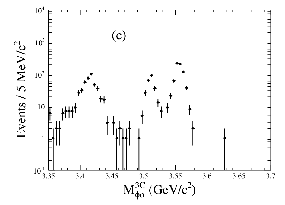
The background from $\psi^{\prime}\to X$ with no radiative photon comes from events where the charged tracks plus a fake photon satisfy the 4C kinematic fit. In the $X$ mass spectrum from a 4C kinematic fit, this background contributes a peak close to the $\eta_{c}^{\prime}$ mass, around $3.656~\mathrm{GeV}/c^{2}$, and decreases sharply at high mass due to the $25~\mathrm{MeV}$ requirement on the photon energy. If the measured energy of the candidate photon is not used in the kinematic fit, thus becoming a 3C fit, this background lies around the $\psi^{\prime}$ mass region ($3.66~\mathrm{GeV}/c^{2}\sim 3.70~\mathrm{GeV}/c^{2}$) in the mass spectrum, as the photon energy from the fit tends to be close to zero energy (see Fig. 1). There is little change in the $\eta_{c}^{\prime}$ mass resolution due to one less constraint in the kinematic fit, but the separation of the $\eta_{c}^{\prime}$ signal from the background is much improved. Therefore, the result from the 3C fit ($M_{X}^{3C}$) is taken as the final mass spectrum.

The background from $\psi^{\prime}\to\pi^{0}X$ is measured from data by reconstructing the $\pi^{0}$ from its decay into two photons. If there are more than two photons, the $\pi^{0}$ candidate is selected as the one with the minimum $\chi^{2}$ from a 5C fit (4C plus a $\pi^{0}$ mass constraint). $\chi^{2}_{5C}<30$ is required to veto backgrounds. A MC sample of $\psi^{\prime}\to\pi^{0}X$ is used to determine the efficiency ratio between events passing the $\psi^{\prime}\to\gamma X$ and $\psi^{\prime}\to\pi^{0}X$ selections. Finally, the efficiency ratio is used to scale the $\psi^{\prime}\to\pi^{0}X$ sample selected from data to obtain the background contamination from $\psi^{\prime}\to\pi^{0}X$ as a function of the $X$ invariant mass. This background, which is described with a Novosibirsk function [18] as shown in Fig. 2, contributes a smooth component in the $\chi_{cJ}$ ($J=0$, 1, 2) mass region ($3.35~\mathrm{GeV}/c^{2}\sim 3.60~\mathrm{GeV}/c^{2}$), and is almost negligible above $3.60~\mathrm{GeV}/c^{2}$.

The background shape from $\psi^{\prime}\to(\gamma_{FSR})X$ is obtained from MC simulation, where the $FSR$ photon is simulated with PHOTOS [19]. The fraction of events with $FSR$ is defined as $R_{FSR}=\frac{N_{\gamma_{FSR}X}}{N_{X}}$, where $N_{\gamma_{FSR}X}$ ($N_{X}$) is the number of events containing an (no) $FSR$ photon that survive selection. This fraction is obtained from measuring the $FSR$ contribution in $\psi^{\prime}\to\gamma\chi_{c0}$, $\chi_{c0}\to(\gamma_{FSR})X$. The event selection of this $FSR$ sample is very similar to that of the signal mode, except that the reconstructed final state contains two photons, where the softer photon is regarded as the $FSR$ photon. The energy of the $FSR$ photon is not used when performing the 3C kinematic fit for this sample. Events from $\psi^{\prime}\to\pi^{0}X$ are the main background for the $FSR$ sample and are excluded by requiring the invariant mass of the two photons to be outside of the $\pi^{0}$ signal region. Figure 3 shows the two-dimensional distribution of $M_{X}^{3C}$ versus $M_{\gamma_{FSR}X}^{3C}$. If we add the four-momenta of the $FSR$ photon and $X$ to calculate the invariant mass for events with $M_{X}^{3C}$ below the $\chi_{c0}$ mass in the PDG ($M_{\chi_{c0}}^{PDG}$), $M_{\gamma_{FSR}X}^{3C}$ peaks at $M_{\chi_{c0}}^{PDG}$ indicating the photon is indeed from $FSR$. As a result, events from $\chi_{c0}\to X$ are in the dashed-line box in Fig. 3, while events from $\chi_{c0}\to\gamma_{FSR}X$ are in the solid-line box in Fig. 3. In this way, we can obtain $R_{FSR}$ for MC simulation and data. The factor $f_{FSR}$ is defined as the ratio of $R_{FSR}$ measured in data to that determined in MC simulation. This $FSR$ measurement is performed for two final states; $f_{FSR}=1.70\pm 0.10$ and $1.39\pm 0.08$ are determined for $X=2(\pi^{+}\pi^{-})$ and $X=\pi^{+}\pi^{-}K^{+}K^{-}$, respectively. The errors are the statistical errors of the sample and the uncertainties of the background estimation. These factors are used to scale fractions of $FSR$ background events [$\psi^{\prime}\to(\gamma_{FSR})X$] in the MC samples to estimate the background in data.

Data taken at $\sqrt{s}=3.773~\mathrm{GeV}$ are used to estimate backgrounds from the continuum [$e^{+}e^{-}\to\gamma^{*}\to(\gamma_{FSR})X$] and initial state radiation ($e^{+}e^{-}\to\gamma_{ISR}X$). MC simulation indicates that $\psi^{\prime\prime}$ decays contribute negligible background in the modes under study. Using the luminosity normalization and energy dependence of the cross section, there are $46\pm 3$ and $8\pm 2$ background events expected for $V=\rho^{0}$ and $V=K^{*0}$, respectively. For $V=\phi$, no events survive the selection.

The signal yields are extracted from an unbinned maximum likelihood fit to the $M_{VV}^{3C}$ distribution. The signal shape is obtained from MC simulation, following $BW(m_{0},\Gamma)\times E_{\gamma}^{3}\times damping$, where $m_{0}$ and $\Gamma$ are the mass and width of the Breit-Wigner for signal and $\chi_{cJ}$, $E_{\gamma}^{3}$ is the cube of the radiative photon energy, which is necessary in an $E1/M1$ radiative transition, and $damping$ stands for a damping function used to damp the diverging tail caused by the $E_{\gamma}^{3}$ at lower mass region (corresponding to a higher energy radiative photon). One damping function used by KEDR [20] is defined as $\frac{E_{0}^{2}}{E_{\gamma}E_{0}+(E_{\gamma}-E_{0})^{2}}$, where $E_{0}$ is the most probable energy of the transition photon. It is also necessary to convolute this with a Gaussian function $G(\mu,\sigma)$ to take the mass resolution difference between MC simulation and data into account. The mean ($\mu$) and standard deviation ($\sigma$) are free parameters for the $\chi_{cJ}$ signals. For $\eta_{c}^{\prime}$, they are fixed to the values extrapolated from $\chi_{cJ}$ with a linear assumption. In the fit, the estimated backgrounds from $\psi^{\prime}\to\pi^{0}X$ and the continuum are fixed. The shape of the $\psi^{\prime}\to(\gamma_{FSR})X$ background comes from the MC simulation. The fraction of MC data with an $FSR$ photon is scaled by the factor $f_{FSR}$ to estimate the fraction of data with $FSR$ background. Figure 4 shows the final fitting results to the 3C mass spectrum. The values of $\chi^{2}/ndf$ are 0.68 and 0.72 for $\rho^{0}\rho^{0}$ and $K^{*0}\bar{K}^{*0}$, respectively, indicating good fits. The numbers of $\eta_{c}^{\prime}$ events obtained are $6.5\pm 6.4$ and $6.9\pm 4.8$ for $V$ = $\rho^{0}$ and $K^{*0}$, respectively. No fit is performed for $\phi\phi$, since there is only one $\eta_{c}^{\prime}\to\phi\phi$ candidate event in the signal region.

The systematic uncertainties related to tracking, photon reconstruction, PID and the kinematic fit are estimated with specially selected control samples [21]. An efficiency can be defined as the ratio of $\chi_{cJ}$ yield for $VV$ with the $V$ mass requirement to that without this requirement. The exact same method is applied to MC and the difference in the efficiency between MC simulation and data is taken as the corresponding systematic uncertainty caused by the $V$ mass requirement, with the statistical error included. An alternative damping function was used by CLEO [22], ${\rm exp}(-E_{\gamma}^{2}/(8\beta^{2}))$, which is inspired by the overlap of wave functions, with $\beta=65.0\pm 2.5~\mathrm{MeV}$ from fitting the $J/\psi\to\gamma\eta_{c}$ photon spectrum. The difference caused by the two damping functions is taken as a systematic uncertainty. The main backgrounds that may affect our fit result in the $\eta_{c}^{\prime}$ mass region are the contributions from $FSR$ in $\psi^{\prime}\to\gamma_{FSR}X$ and from the continuum. Therefore, the systematic uncertainty from the background shape is estimated by changing the $FSR$ and continuum contributions by $1\sigma$. There are also systematic uncertainties related to the mass and width of the $\eta_{c}^{\prime}$, which are estimated by comparing the $\eta_{c}^{\prime}$ yields with the mass and width fixed to the center values or randomly selected values according to a Gaussian distribution. Table 1 shows a summary of all the systematic uncertainties.

As there is no significant $\eta_{c}^{\prime}$ signal in any of the three final states, we determine upper limits on the $\psi^{\prime}\to\gamma\eta_{c}^{\prime}\to\gamma VV$ production rates. We assume all the signal events from the fit are due to $\eta_{c}^{\prime}\to VV$, neglecting possible interference between the signal and nonresonant contributions. The probability density function (PDF) for the expected number of signal events is smeared with the systematic uncertainties (by convolution). For $V=\rho^{0}$ and $K^{*0}$, the PDF is taken to be the likelihood distribution in fitting the invariant mass distributions in Fig. 4 by setting the number of $\eta_{c}^{\prime}$ signal events from zero up to a very large number. For $V=\phi$, the one event in the $\eta_{c}^{\prime}$ mass region is taken as signal for simplicity, and the PDF is assumed to be a Poisson distribution.

The upper limit on the number of events at the 90% C.L., $N^{up}_{\gamma VV}$, corresponds to ${\int_{0}^{N^{up}_{\gamma VV}}{\rm PDF}(x)dx}/{\int_{0}^{\infty}{\rm PDF}(x)dx}=0.90$ on the smeared PDF. The left half of Table 2 shows $N^{up}$, the efficiencies from MC simulation, and the upper limits on the product branching fraction $\mathcal{B}$($\psi^{\prime}\to\gamma\eta_{c}^{\prime})\times\mathcal{B}(\eta_{c}^{\prime}\to VV)$. Using $\mathcal{B}(\psi^{\prime}\to\gamma\eta_{c}^{\prime})=(4.7\pm 0.9\pm 3.0)\times 10^{-4}$ [4], the corresponding upper limits on $\mathcal{B}(\eta_{c}^{\prime}\to VV)$ are listed in the right half of Table 2. In calculating $\mathcal{B}^{up}(\eta_{c}^{\prime}\to VV)$, the error on $\mathcal{B}(\psi^{\prime}\to\gamma\eta_{c}^{\prime})$ is taken as a systematic uncertainty to smear the PDF. The theoretical predictions [6] on branching fractions for $\eta_{c}^{\prime}\to VV$, which are calculated with $\Gamma_{\eta_{c}^{\prime}}=10.4\pm 4.2~\mathrm{MeV}$ [23], are also listed in Table 2.

In conclusion, no obvious $\eta_{c}^{\prime}$ signal was observed in decays into vector meson pairs: $\rho^{0}\rho^{0}$, $K^{*0}\bar{K}^{*0}$, and $\phi\phi$. The upper limits on the product branching fraction $\mathcal{B}(\psi^{\prime}\to\gamma\eta_{c}^{\prime})\times\mathcal{B}(\eta_{c}^{\prime}\to VV)$ and $\eta_{c}^{\prime}$ decay branching fraction $\mathcal{B}(\eta_{c}^{\prime}\to VV)$ are determined. These upper limits are smaller than the lower bounds of the theoretical predictions [6], although the difference is very small for $\eta_{c}^{\prime}\to\phi\phi$.

The BESIII Collaboration thanks the staff of BEPCII and the computing center for their hard efforts. This work is supported in part by the Ministry of Science and Technology of China under Contract No. 2009CB825200; National Natural Science Foundation of China (NSFC) under Contracts No. 10625524, No. 10821063, No. 10825524, No. 10835001, No. 10935007; the Chinese Academy of Sciences (CAS) Large-Scale Scientific Facility Program; CAS under Contracts No. KJCX2-YW-N29, No. KJCX2-YW-N45; 100 Talents Program of CAS; Istituto Nazionale di Fisica Nucleare, Italy; Siberian Branch of Russian Academy of Science, joint project No. 32 with CAS; U. S. Department of Energy under Contracts No. DE-FG02-04ER41291, No. DE-FG02-91ER40682, No. DE-FG02-94ER40823; University of Groningen (RuG) and the Helmholtzzentrum fuer Schwerionenforschung GmbH (GSI), Darmstadt; WCU Program of National Research Foundation of Korea under Contract No. R32-2008-000-10155-0.

References

- [1] S. K. Choi et al. (Belle Collaboration), Phys. Rev. Lett. 89, 102001 (2002).
- [2] D. M. Asner et al. (CLEO Collaboration), Phys. Rev. Lett. 92, 142001 (2004); B. Aubert et al. (BaBar Collaboration), Phys. Rev. Lett. 92, 142002 (2004); B. Aubert et al. (BaBar Collaboration), Phys. Rev. D 72, 031101 (2005).
- [3] A. Vinokurova et al. (Belle Collaboration), arXiv:1105.0978v2; P. del Amo Sanchez et al. (BaBar Collaboration), Phys. Rev. D 84, 012004 (2011); H. Nakazawa (Belle Collaboration), in Proc. Sci. ICHEP2010 (2010) 162.
- [4] L. L. Wang (for the BESIII Collaboration), arXiv:1110.2560 [hep-ex], talk at the “XIV International Conference on Hadron Spectroscopy”, 13-17 June, 2011, Munchen, Germany.
- [5] S. J. Brodsky and G. P. Lepage, Phys. Rev. D 24, 2848 (1981); V. L. Chernyak and A. R. Zhitnitsky, Nucl. Phys. B 201, 492 (1982); V. L. Chernyak and A. R. Zhitnitsky, Phys. Rept. 112, 173 (1984).
- [6] Q. Wang, X. H. Liu and Q. Zhao, arXiv:1010.1343.
- [7] X. H. Liu and Q. Zhao, Phys. Rev. D 81, 014017 (2010); X. H. Liu and Q. Zhao, arXiv:1004.0496.
- [8] Q. Zhao et al., Chinese Phys. C 34, 299 (2010); Q. Zhao, arXiv:1012.2887.
- [9] X. H. Mo, C. Z. Yuan, and P. Wang, High Energy Phys. Nucl. Phys. 31, 686 (2007) [arXiv:hep-ph/0611214].
- [10] M. Ablikim et al. (BESIII Collaboration), Phys. Rev. D 81, 052005 (2010).
- [11] M. Ablikim et al. (BESIII Collaboration), Nucl. Instrum. Methods Phys. Res., Sect. A 614, 345 (2010).
- [12] S. Agostinelli et al., Nucl. nstrum. Methods Phyd. Res. Sect. A, 506, 250 (2003).
- [13] J. C. Chen, G. S. Huang, X. R. Qi, D. H. Zhang and Y. S. Zhu, Phys. Rev. D 62, 034003 (2000).
- [14] K. Nakamura et al. (Particle Data Group), J. Phys. G 37, 075021 (2010).
- [15] The amplitudes and phases for H+, H0, and H- are 1.0, 0.0, 0.0, 0.0, -1.0, 0.0, which are calculated by requring of -parity conservation for the allowed components of helicity amplitudes.
- [16] D. J. Lange, Nucl. Instrum. Methods Phys. Res., Sect. A 462, 152 (2001).
- [17] The recoil mass is defined as , where and are energy and momentum for a particle.
- [18] The Novosibirsk function is defined as , where , the peak position is , the width is , and is the tail parameter.
- [19] E. Barberio and Z. Was, Comput. Phys. Commun. 79, 291 (1994).
- [20] V. V. Anashin et al., arXiv:1012.1694.
- [21] M. Ablikim et al. (BESIII Collaboration), Phys. Rev. D 83, 112005 (2011); Phys. Rev. Lett. 107, 092001 (2011).
- [22] R. E. Mitchell et al. (CLEO Collaboration), Phys. Rev. Lett. 102, 011801 (2009); R. E. Mitchell et al. (CLEO Collaboration), Phys. Rev. Lett. 106, 159903 (2011).
- [23] By averaging measurements listed by the PDG [14] and recent results from BaBar and Belle, we determine the mass , and the width .