Width Distributions for Convex Regular Polyhedra

Given a convex region $C$ in $\mathbb{R}^{2}$, a width is the distance between a pair of parallel $C$-supporting lines. Every unit vector $u\in\mathbb{R}^{2}$ determines a unique such pair of lines orthogonal to $u$ and hence a width $w(u)$. Let $u$ be uniformly distributed on the unit circle $S^{1}\subset$ $\mathbb{R}^{2}$. We wish to study the distribution of the random variable $w$ in the case $C=$ the equilateral triangle with sides of unit length.

For simplicity, let $\triangle$ be the equilateral triangle with vertices

$$\begin{array}[c]{ccccc}v_{1}=\left(0,1\right),&&v_{2}=\left(\frac{\sqrt{3}}{2},-\frac{1}{2}\right),&&v_{3}=\left(-\frac{\sqrt{3}}{2},-\frac{1}{2}\right).\end{array}$$

At the end, it will be necessary to normalize by $\sqrt{3}$, the side-length of $\triangle$.

Also let $\widetilde{\triangle}$ be the union of three overlapping disks of radius $1/2$ centered at $v_{1}/2$, $v_{2}/2$, $v_{3}/2$. Clearly $\triangle\subset\widetilde{\triangle}$ and $\widetilde{\triangle}$ has centroid $(0,0)$. A diameter of $\widetilde{\triangle}$ is the length of the intersection between $\widetilde{\triangle}$ and a line passing through the origin.

Computing all widths of $\triangle$ is equivalent to computing all diameters of $\widetilde{\triangle}$. The latter is achieved as follows. Fix a point $(a,b)$ on the unit circle. The line $L$ passing through $(0,0)$ and $(a,b)$ has parametric representation

$$\begin{array}[c]{ccccc}x=t\,a,&&y=t\,b,&&t\in\mathbb{R}\end{array}$$

and hence $y=(b/a)x$ assuming $a\neq 0$. The nontrivial intersection between top circle and $L$ satisfies

$$x^{2}+\left(\tfrac{b}{a}x-\tfrac{1}{2}\right)^{2}=\tfrac{1}{4}$$

thus $x_{1}=a\,b$ since $a^{2}+b^{2}=1$. The nontrivial intersection between right circle and $L$ satisfies

$$\left(x-\tfrac{\sqrt{3}}{4}\right)^{2}+\left(\tfrac{b}{a}x+\tfrac{1}{4}\right)^{2}=\tfrac{1}{4}$$

thus $x_{2}=a\left(\sqrt{3}a-b\right)/2$ . The nontrivial intersection between left circle and $L$ satisfies

$$\left(x+\tfrac{\sqrt{3}}{4}\right)^{2}+\left(\tfrac{b}{a}x+\tfrac{1}{4}\right)^{2}=\tfrac{1}{4}$$

thus $x_{3}=-a\left(\sqrt{3}a+b\right)/2$ .

We now examine all pairwise distances, squared, between the three intersection points:

$$\left(x_{i}-x_{j}\right)^{2}+\left(\tfrac{b}{a}x_{i}-\tfrac{b}{a}x_{j}\right)^{2}=\left\{\begin{array}[c]{lll}\frac{1}{4}\left(3-6\sqrt{3}a\,b+6b^{2}\right)&&\text{if }i=1,j=2\\ \frac{3}{4}\left(1+2\sqrt{3}a\,b+2b^{2}\right)&&\text{if }i=1,j=3\\ 3a^{2}&&\text{if }i=2,j=3\end{array}\right.$$

and define

$$g(a,b)=\max\left\{\tfrac{1}{4}\left(3-6\sqrt{3}a\,b+6b^{2}\right),\tfrac{3}{4}\left(1+2\sqrt{3}a\,b+2b^{2}\right),3a^{2}\right\}.$$

Therefore the mean width for $C$ is

$$\frac{1}{\sqrt{3}}\frac{1}{2\pi}{\displaystyle\int\limits_{0}^{2\pi}}\sqrt{g(\cos\theta,\sin\theta)}\,d\theta=\frac{3}{\pi}=\frac{\text{perimeter of }C}{\pi}$$

and the mean square width is

$$\frac{1}{3}\frac{1}{2\pi}{\displaystyle\int\limits_{0}^{2\pi}}g(\cos\theta,\sin\theta)\,d\theta=\frac{1}{2}\left(1+\frac{3\sqrt{3}}{2\pi}\right).$$

We turn to the case $C=$ the square with sides of unit length. For simplicity, let $\square$ be the square with vertices

$$\begin{array}[c]{ccccccc}v_{1}=\left(\frac{\sqrt{2}}{2},\frac{\sqrt{2}}{2}\right),&&v_{2}=\left(\frac{\sqrt{2}}{2},-\frac{\sqrt{2}}{2}\right),&&v_{3}=\left(-\frac{\sqrt{2}}{2},\frac{\sqrt{2}}{2}\right),&&v_{4}=\left(-\frac{\sqrt{2}}{2},-\frac{\sqrt{2}}{2}\right).\end{array}$$

At the end, it will be necessary to normalize by $\sqrt{2}$, the side-length of $\square$.

Also let $\widetilde{\square}$ be the union of four overlapping disks of radius $1/2$ centered at $v_{1}/2$, $v_{2}/2$, $v_{3}/2$, $v_{4}/2$. A diameter of $\widetilde{\square}$ is the length of the intersection between $\widetilde{\square}$ and a line passing through the origin.

Computing all widths of $\square$ is equivalent to computing all diameters of $\widetilde{\square}$. Fix a point $(a,b)$ on the unit circle. The line $L$ passing through $(0,0)$ and $(a,b)$ can be represented as $y=(b/a)x$ assuming $a\neq 0$. The nontrivial intersection between northeast circle and $L$ satisfies

$$\left(x-\tfrac{\sqrt{2}}{4}\right)^{2}+\left(\tfrac{b}{a}x-\tfrac{\sqrt{2}}{4}\right)^{2}=\tfrac{1}{4}$$

thus $x_{1}=\sqrt{2}a(a+b)/2$ since $a^{2}+b^{2}=1$. The nontrivial intersection between southeast circle and $L$ satisfies

$$\left(x-\tfrac{\sqrt{2}}{4}\right)^{2}+\left(\tfrac{b}{a}x+\tfrac{\sqrt{2}}{4}\right)^{2}=\tfrac{1}{4}$$

thus $x_{2}=\sqrt{2}a(a-b)/2$. The nontrivial intersection between northwest circle and $L$ satisfies

$$\left(x+\tfrac{\sqrt{2}}{4}\right)^{2}+\left(\tfrac{b}{a}x-\tfrac{\sqrt{2}}{4}\right)^{2}=\tfrac{1}{4}$$

thus $x_{3}=-\sqrt{2}a(a-b)/2$. The nontrivial intersection between southwest circle and $L$ satisfies

$$\left(x+\tfrac{\sqrt{2}}{4}\right)^{2}+\left(\tfrac{b}{a}x+\tfrac{\sqrt{2}}{4}\right)^{2}=\tfrac{1}{4}$$

thus $x_{4}=-\sqrt{2}a(a+b)/2$.

We now examine all pairwise distances, squared, between the four intersection points:

$$\left(x_{i}-x_{j}\right)^{2}+\left(\tfrac{b}{a}x_{i}-\tfrac{b}{a}x_{j}\right)^{2}=\left\{\begin{array}[c]{lll}2b^{2}&&\text{if }i=1,j=2\\ 2a^{2}&&\text{if }i=1,j=3\\ 2+4a\,b&&\text{if }i=1,j=4\\ 2-4a\,b&&\text{if }i=2,j=3\\ 2a^{2}&&\text{if }i=2,j=4\\ 2b^{2}&&\text{if }i=3,j=4\end{array}\right.$$

and define

	$\displaystyle g(a,b)$	$\displaystyle=\max\left\{2a^{2},2b^{2},2(1+2a\,b),2(1-2a\,b)\right\}$
		$\displaystyle=\max\left\{2(1+2a\,b),2(1-2a\,b)\right\}.$

Therefore the mean width for $C$ is

$$\frac{1}{\sqrt{2}}\frac{1}{2\pi}{\displaystyle\int\limits_{0}^{2\pi}}\sqrt{g(\cos\theta,\sin\theta)}\,d\theta=\frac{4}{\pi}=\frac{\text{perimeter of }C}{\pi}$$

and the mean square width is

$$\frac{1}{2}\frac{1}{2\pi}{\displaystyle\int\limits_{0}^{2\pi}}g(\cos\theta,\sin\theta)\,d\theta=1+\frac{2}{\pi}.$$

Returning to the three-dimensional setting of the introduction, let $C=$ the regular tetrahedron with edges of unit length.

For simplicity, let $\triangle$ be the tetrahedron with vertices

$$\begin{array}[c]{lll}v_{1}=\left(0,0,1\right),&&v_{2}=\left(\frac{2\sqrt{2}}{3},0,-\frac{1}{3}\right),\\ v_{3}=\left(-\frac{\sqrt{2}}{3},\sqrt{\frac{2}{3}},-\frac{1}{3}\right),&&v_{4}=\left(-\frac{\sqrt{2}}{3},-\sqrt{\frac{2}{3}},-\frac{1}{3}\right),\end{array}$$

At the end, it will be necessary to normalize by $2\sqrt{2/3}$, the edge-length of $\triangle$.

Also let $\widetilde{\triangle}$ be the union of four overlapping balls of radius $1/2$ centered at $v_{1}/2$, $v_{2}/2$, $v_{3}/2$, $v_{4}/2$. Clearly $\triangle\subset\widetilde{\triangle}$ and $\widetilde{\triangle}$ has centroid $(0,0,0)$. A diameter of $\widetilde{\triangle}$ is the length of the intersection between $\widetilde{\triangle}$ and a line passing through the origin.

Computing all widths of $\triangle$ is equivalent to computing all diameters of $\widetilde{\triangle}$. The latter is achieved as follows. Fix a point $(a,b,c)$ on the unit sphere. The line $L$ passing through $(0,0,0)$ and $(a,b,c)$ has parametric representation

$$\begin{array}[c]{ccccccc}x=t\,a,&&y=t\,b,&&z=t\,c,&&t\in\mathbb{R}\end{array}$$

and hence $y=(b/a)x$, $z=(c/a)x$ assuming $a\neq 0$. The nontrivial intersection between top sphere and $L$ satisfies

$$x^{2}+\left(\tfrac{b}{a}x\right)^{2}+\left(\tfrac{c}{a}x-\tfrac{1}{2}\right)^{2}=\tfrac{1}{4}$$

thus $x_{1}=a\,c$ since $a^{2}+b^{2}+c^{2}=1$. The nontrivial intersection between front sphere and $L$ satisfies

$$\left(x-\tfrac{\sqrt{2}}{3}\right)^{2}+\left(\tfrac{b}{a}x\right)^{2}+\left(\tfrac{c}{a}x+\tfrac{1}{6}\right)^{2}=\tfrac{1}{4}$$

thus $x_{2}=a\left(2\sqrt{2}a-c\right)/3$ . The nontrivial intersection between left sphere and $L$ satisfies

$$\left(x+\tfrac{\sqrt{2}}{6}\right)^{2}+\left(\tfrac{b}{a}x+\tfrac{\sqrt{6}}{6}\right)^{2}+\left(\tfrac{c}{a}x+\tfrac{1}{6}\right)^{2}=\tfrac{1}{4}$$

thus $x_{3}=-a\left(\sqrt{2}a+\sqrt{6}b+c\right)/3$. The nontrivial intersection between right sphere and $L$ satisfies

$$\left(x+\tfrac{\sqrt{2}}{6}\right)^{2}+\left(\tfrac{b}{a}x-\tfrac{\sqrt{6}}{6}\right)^{2}+\left(\tfrac{c}{a}x+\tfrac{1}{6}\right)^{2}=\tfrac{1}{4}$$

thus $x_{4}=a\left(-\sqrt{2}a+\sqrt{6}b-c\right)/3$.

We now examine all pairwise distances, squared, between the four intersection points:

		$\displaystyle\left(x_{i}-x_{j}\right)^{2}+\left(\tfrac{b}{a}x_{i}-\tfrac{b}{a}x_{j}\right)^{2}+\left(\tfrac{c}{a}x_{i}-\tfrac{c}{a}x_{j}\right)^{2}$
		$\displaystyle=\left\{\begin{array}[c]{lll}\frac{8}{9}\left(a^{2}-2\sqrt{2}a\,c+2c^{2}\right)&&\text{if }i=1,j=2\\ \tfrac{1}{9}\left(\sqrt{2}a+\sqrt{6}b+4c\right)^{2}&&\text{if }i=1,j=3\\ \tfrac{1}{9}\left(\sqrt{2}a-\sqrt{6}b+4c\right)^{2}&&\text{if }i=1,j=4\\ \frac{2}{3}\left(3a^{2}+2\sqrt{3}a\,b+b^{2}\right)&&\text{if }i=2,j=3\\ \frac{2}{3}\left(3a^{2}-2\sqrt{3}a\,b+b^{2}\right)&&\text{if }i=2,j=4\\ \frac{8}{3}b^{2}&&\text{if }i=3,j=4\end{array}\right.$

and define

	$\displaystyle g(a,b)$	$\displaystyle=\max\left\{\tfrac{8}{9}\left(a^{2}-2\sqrt{2}a\,c+2c^{2}\right),\tfrac{1}{9}\left(\sqrt{2}a+\sqrt{6}b+4c\right)^{2},\tfrac{1}{9}\left(\sqrt{2}a-\sqrt{6}b+4c\right)^{2},\right.$
		$\displaystyle\left.\;\;\;\;\;\;\;\;\;\tfrac{2}{3}\left(3a^{2}+2\sqrt{3}a\,b+b^{2}\right),\tfrac{2}{3}\left(3a^{2}-2\sqrt{3}a\,b+b^{2}\right),\tfrac{8}{3}b^{2}\right\}.$

As for the equilateral triangle, no simplication of $g$ seems possible. The mean width for $C$ is

$$\frac{1}{2\sqrt{2/3}}\frac{1}{4\pi}{\displaystyle\int\limits_{0}^{2\pi}}{\displaystyle\int\limits_{0}^{\pi}}\sqrt{g(\cos\theta\sin\varphi,\sin\theta\sin\varphi,\cos\varphi)}\sin\varphi\,d\varphi\,d\theta=\frac{3}{2\pi}\arccos\left(-\frac{1}{3}\right)$$

and the mean square width is

$$\frac{1}{8/3}\frac{1}{4\pi}{\displaystyle\int\limits_{0}^{2\pi}}{\displaystyle\int\limits_{0}^{\pi}}g(\cos\theta\sin\varphi,\sin\theta\sin\varphi,\cos\varphi)\sin\varphi\,d\varphi\,d\theta=\frac{1}{3}\left(1+\frac{3+\sqrt{3}}{\pi}\right).$$

Details on the final integral are given in Section 5.

We turn to the case $C=$ the cube with edges of unit length. For simplicity, let $\square$ be the cube with vertices

$$v_{k}=\left(\pm\tfrac{\sqrt{3}}{3},\pm\tfrac{\sqrt{3}}{3},\pm\tfrac{\sqrt{3}}{3}\right)$$

for $1\leq k\leq 8$. At the end, it will be necessary to normalize by $2/\sqrt{3}$, the edge-length of $\square$.

Also let $\widetilde{\square}$ be the union of eight overlapping balls of radius $1/2$ centered at $v_{1}/2$, $v_{2}/2$, $v_{3}/2$, …, $v_{8}/2$. A diameter of $\widetilde{\square}$ is the length of the intersection between $\widetilde{\square}$ and a line passing through the origin.

Computing all widths of $\square$ is equivalent to computing all diameters of $\widetilde{\square}$. Fix a point $(a,b,c)$ on the unit sphere. The line $L$ passing through $(0,0,0)$ and $(a,b,c)$ can be represented as $y=(b/a)x$, $z=(c/a)x$ assuming $a\neq 0$. The nontrivial intersection between each of the eight spheres and $L$ satisfies

$$\left(x\pm\tfrac{\sqrt{3}}{6}\right)^{2}+\left(\tfrac{b}{a}x\pm\tfrac{\sqrt{3}}{6}\right)^{2}+\left(\tfrac{c}{a}x\pm\tfrac{\sqrt{3}}{6}\right)^{2}=\tfrac{1}{4}$$

and consequently

	$\displaystyle g(a,b)$	$\displaystyle=\max\left\{\tfrac{4}{3}a^{2},\tfrac{4}{3}b^{2},\tfrac{4}{3}c^{2},\tfrac{4}{3}\left(1+2a\,b-c^{2}\right),\tfrac{4}{3}\left(1+2a\,c-b^{2}\right),\right.$
		$\displaystyle\;\;\;\;\;\;\;\;\;\tfrac{4}{3}\left(1-2a\,b-c^{2}\right),\tfrac{4}{3}\left(1-2a\,c-b^{2}\right),\tfrac{4}{3}\left(b+c\right)^{2},\tfrac{4}{3}\left(b-c\right)^{2},$
		$\displaystyle\;\;\;\;\;\;\;\;\;\tfrac{4}{3}\left(1+2a\,b+2a\,c+2b\,c\right),\tfrac{4}{3}\left(1+2a\,b-2a\,c-2b\,c\right),$
		$\displaystyle\left.\;\;\;\;\;\;\;\;\,\tfrac{4}{3}\left(1-2a\,b-2a\,c+2b\,c\right),\tfrac{4}{3}\left(1-2a\,b+2a\,c-2b\,c\right)\right\}$

after examining all 28 pairwise distances and extracting 13 distinct expressions. As for the square (in which $g$ simplified to a maximum over two terms), here $g$ simplifies to a maximum over four terms:

	$\displaystyle g(a,b)$	$\displaystyle=\max\left\{\tfrac{4}{3}\left(1+2a\,b+2a\,c+2b\,c\right),\tfrac{4}{3}\left(1+2a\,b-2a\,c-2b\,c\right),\right.$
		$\displaystyle\left.\;\;\;\;\;\;\;\;\;\tfrac{4}{3}\left(1-2a\,b-2a\,c+2b\,c\right),\tfrac{4}{3}\left(1-2a\,b+2a\,c-2b\,c\right)\right\}.$

The mean width for $C$ is

$$\frac{1}{2/\sqrt{3}}\frac{1}{4\pi}{\displaystyle\int\limits_{0}^{2\pi}}{\displaystyle\int\limits_{0}^{\pi}}\sqrt{g(\cos\theta\sin\varphi,\sin\theta\sin\varphi,\cos\varphi)}\sin\varphi\,d\varphi\,d\theta=\frac{3}{2}$$

and the mean square width is

$$\frac{1}{4/3}\frac{1}{4\pi}{\displaystyle\int\limits_{0}^{2\pi}}{\displaystyle\int\limits_{0}^{\pi}}g(\cos\theta\sin\varphi,\sin\theta\sin\varphi,\cos\varphi)\sin\varphi\,d\varphi\,d\theta=1+\frac{4}{\pi}.$$

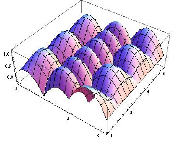
Considerable work is required to evaluate the definite integral at the end of Section 3. A plot of the surface

$$(\theta,\varphi)\longmapsto\sqrt{\frac{g(\cos\theta\sin\varphi,\sin\theta\sin\varphi,\cos\varphi)}{8/3}}$$

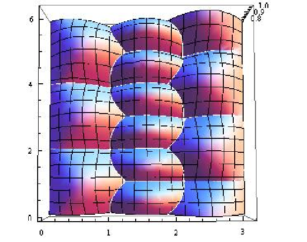
appears in Figure 1, where $0\leq\theta\leq 2\pi$ and $0\leq\varphi\leq\pi$. Figure 2 contains the same surface, but viewed from above. Our focus will be on the part of the surface in the lower right corner, specifically $0\leq\theta\leq\pi/3$ and $2\lessapprox\varphi\leq\pi$. The volume under this part is $1/24^{\text{th}}$ of the volume under the full surface.

We need to find the precise lower bound on $\varphi$ as a function of $\theta$. Recall the formula for $g$ as a maximum over six terms in Section 3; let $g_{\ell}$ denote the $\ell^{\text{th}}$ term, where $1\leq\ell\leq 6$. Then the lower bound on $\varphi$ is found by solving the equation

$$g_{1}(\cos\theta\sin\varphi,\sin\theta\sin\varphi,\cos\varphi)=g_{4}(\cos\theta\sin\varphi,\sin\theta\sin\varphi,\cos\varphi)$$

for $\varphi$. We obtain $\varphi(\theta)=2\arctan(h(\theta))$, where

$$h(\theta)=\frac{\cos\theta+\sqrt{3}\sin\theta+\sqrt{10-\cos(2\theta)+\sqrt{3}\sin(2\theta)}}{2\sqrt{2}}$$

and, in particular,

$$\varphi(0)=2\arctan\left(\sqrt{2}\right)\approx 1.9106,$$

$$\varphi(\pi/3)=2\arctan\left(\left(1+\sqrt{3}\right)/\sqrt{2}\right)\approx 2.1862.$$

It follows that $g=g_{1}$ for $0\leq\theta\leq\pi/3$ and $2\arctan(h)\leq\varphi\leq\pi$. Now we have

		$\displaystyle\frac{1}{8/3}\frac{1}{4\pi}{\displaystyle\int}g_{1}(\cos\theta\sin\varphi,\sin\theta\sin\varphi,\cos\varphi)\sin\varphi\,d\varphi$
		$\displaystyle=\frac{\left(-3+\cos(2\theta)\right)\cos(3\varphi)-3\left(7+3\cos(2\theta)\right)\cos\varphi-16\sqrt{2}\cos\theta\sin^{3}\varphi}{288\pi}$

and

$$\left.\cos(3\varphi)\right|_{2\arctan(h)}^{\pi}=-2\frac{\left(1-3h^{2}\right)^{2}}{(1+h^{2})^{3}},$$

$$\begin{array}[c]{ccc}\left.\cos(\varphi)\right|_{2\arctan(h)}^{\pi}=-\dfrac{2}{1+h^{2}},&&\left.\sin(\varphi)\right|_{2\arctan(h)}^{\pi}=-\dfrac{2h}{1+h^{2}}\end{array}$$

therefore

		$\displaystyle\frac{1}{8/3}\frac{1}{4\pi}{\displaystyle\int_{2\arctan(h)}^{\pi}}g_{1}(\cos\theta\sin\varphi,\sin\theta\sin\varphi,\cos\varphi)\sin\varphi\,d\varphi$
		$\displaystyle=\frac{6h^{4}+8\sqrt{2}h^{3}\cos(\theta)+3h^{2}\left(1+\cos(2\theta)\right)+\left(3+\cos(2\theta)\right)}{18\pi(1+h^{2})^{3}}.$

Integrating this expression from $0$ to $\pi/3$ gives the desired formula for $\operatorname*{E}\left(w_{\text{tetra}}^{2}\right)$.