Computation of Object Approach by a Biophysical Model of a Wide-Field Visual Neuron: Dynamics, Peaks, & Fits

Collision sensitive neurons were reported in species such different as monkeys [5, 4], pigeons [36, 34], frogs [16, 20], and insects [33, 26, 27, 10, 38]. This indicates a high ecological relevance, and raises the question about how neurons compute a signal that eventually triggers corresponding movement patterns (e.g. escape behavior or interceptive actions). Here, we will focus on visual stimulation. Consider, for simplicity, a circular object (diameter $2l$), which approaches the eye at a collision course with constant velocity $v$. If we do not have any a priori knowledge about the object in question (e.g. its typical size or speed), then we will be able to access only two information sources. These information sources can be measured at the retina and are called optical variables (OVs). The first is the visual angle $\Theta$, which can be derived from the number of stimulated photoreceptors (spatial contrast). The second is its rate of change $d\Theta(t)/dt\equiv\dot{\Theta}(t)$. Angular velocity $\dot{\Theta}$ is related to temporal contrast.
How should we combine $\Theta$ and $\dot{\Theta}$ in order to track an imminent collision? The perhaps simplest combination is $\tau(t)\equiv\Theta(t)/\dot{\Theta}(t)$ [13, 18]. If the object hit us at time $t_{c}$, then $\tau(t)\approx t_{c}-t$ will give us a running estimation of the time that is left until contact¹¹ 1 This linear approximation gets worse with increasing $\Theta$, but turns out to work well until short before ttc.. Moreover, we do not need to know anything about the approaching object: The ttc estimation computed by $\tau$ is independent of object size and velocity. Neurons with $\tau$-like responses were indeed identified in the nucleus retundus of the pigeon brain [34]. In humans, only fast interceptive actions seem to rely exclusively on $\tau$ [37, 35]. Accurate ttc estimation, however, seems to involve further mechanisms (rate of disparity change [31]).
Another function of OVs with biological relevance is $\eta\equiv\dot{\Theta}\exp(-\alpha\Theta)$, with $\alpha=const.$ [10]. While $\eta$-type neurons were found again in pigeons [34] and bullfrogs [20], most data were gathered from the LGMD²² 2 LGMD activity is usually monitored via its postsynaptic neuron, the Descending Contralateral Movement Detector (DCMD) neuron. This represents no problem as LGMD spikes follow DCMD spikes 1:1 under visual stimulation [22] from 300Hz [21] to at least 400Hz [24]. in locusts (e.g. [10, 9, 7, 23]). The $\eta$-function is a phenomenological model for the LGMD, and implies three principal hypothesis: (i) An implementation of an exponential function $\exp(\cdot)$. Exponentation is thought to take place in the LGMD axon, via active membrane conductances [8]. Experimental data, though, seem to favor a third-power law rather than $\exp(\cdot)$. (ii) The LGMD carries out biophysical computations for implementing the multiplicative operation. It has been suggested that multiplication is done within the LGMD itself, by subtracting the logarithmically encoded variables $\log\dot{\Theta}-\alpha\Theta$ [10, 8]. (iii) The peak of the $\eta$-function occurs before ttc, at visual angle $\Theta(\hat{t})=2\arctan(1/\alpha)$ [9]. It follows ttc for certain stimulus configurations (e.g. $l/|v|\lessapprox 5ms$). In principle, $\hat{t}>t_{c}$ can be accounted for by $\eta(t+\delta)$ with a fixed delay $\delta<0$ (e.g. $-27ms$). But other researchers observed that LGMD activity continuous to rise after ttc even for $l/|v|\gtrapprox 5ms$ [28]. These discrepancies remain unexplained so far [29], but stimulation dynamics perhaps plays a role.
We we will address these three issues by comparing the novel function “$\psi$” with the $\eta$-function.

A circular object which starts its approach at distance $x_{0}$ and with speed $v$ projects a visual angle $\Theta(t)=2\arctan[l/(x_{0}-vt)]$ on the retina [34, 9]. The kinematics is hence entirely specified by the half-size-to-velocity ratio $l/|v|$, and $x_{0}$. Furthermore, $\dot{\Theta}(t)=2lv/((x_{0}-vt)^{2}+l^{2})$.
In order to define $\psi$, we consider at first the LGMD neuron as an RC-circuit with membrane potential³³ 3 Here we assume that the membrane potential serves as a predictor for the LGMD’s mean firing rate. $V$ [17]

$C_{m}$ $=$ membrane capacity⁴⁴ 4 Set to unity for all simulations; $\beta\equiv 1/R_{m}$ denotes leakage conductance across the cell membrane ($R_{m}$: membrane resistance); $g_{exc}$ and $g_{inh}$ are excitatory and inhibitory inputs. Each conductance $g_{i}$ ($i=\mathit{rest},\mathit{exc},\mathit{inh}$) can drive the membrane potential to its associated reversal potential $V_{i}$ (usually $V_{inh}\leq V_{exc}$). Shunting inhibition means $V_{i}=V_{rest}$. Shunting inhibition lurks “silently” because it gets effective only if the neuron is driven away from its resting potential. With synaptic input, the neuron decays into its equilibrium state $V_{\infty}\equiv(V_{rest}\beta+V_{exc}g_{exc}+V_{inh}g_{inh})/(\beta+g_{exc}+g_{inh})$ according to $V(t)=V_{\infty}(1-exp(-t/\tau_{m}))$. Without external input, $V(t\gg 1)\rightarrow V_{rest}$. The time scale is set by $\tau_{m}$. Without synaptic input $\tau_{m}\equiv C_{m}/\beta$. Slowly varying inputs $g_{exc},g_{inh}>0$ modify the time scale to approximately $\tau_{m}/(1+(g_{exc}+g_{inh})/\beta)$. For highly dynamic inputs, such as in late phase of the object approach, the time scale gets dynamical as well. The $\psi$-model assigns synaptic inputs⁵⁵ 5 LGMD receives also inhibition from a laterally acting network [21]. The $\eta$-function considers only direct feedforward inhibition [22, 6], and so do we.

Thus, we say $\psi(t)\equiv V(t)$ if and only if $g_{exc}$ and $g_{inh}$ are defined with the last equation. The time scale of stimulation is defined by $\Delta t_{sim}$ (by default $1ms$). The variables $\vartheta$ and $\dot{\vartheta}$ are lowpass filtered angular size and rate of expansion, respectively. The amount of filtering is defined by memory constants $\zeta_{0}$ and $\zeta_{1}$ (no filtering for zero). The idea is to continue to generate synaptic input after ttc, where $\Theta(t>t_{c})=const$ and thus $\dot{\Theta}(t>t_{c})=0$. Inhibition is first weighted by $\gamma$, and then potentiated by the exponent $e$. Hodgkin-Huxley potentiates gating variables $n,m\in[0,1]$ instead (potassium $\propto n^{4}$, sodium $\propto m^{3}$, [12]) and multiplies them with conductances. Gabbiani and co-workers found that the function which transforms membrane potential to firing rate is better described by a power function with $e=3$ than by $\exp(\cdot)$ (Figure 4d in [8]).

Discretization. In a typical experiment, a monitor is placed a short distance away form the insect’s eye, and an approaching object is displayed. Computer screens have a fixed spatial resolution, and as a consequence size increments of the displayed object proceed in discrete jumps. The locust retina is furthermore composed of a discrete array of ommatidia units. We therefore can expect a corresponding step-wise increment of $\Theta$ with time, although optical and neuronal filtering may smooth $\Theta$ to some extent again, resulting in $\vartheta$ (figure 1). Discretization renders $\dot{\Theta}$ discontinuous, what again will be alleviated in $\dot{\vartheta}$. For simulating the dynamics of $\psi$, we discretized angular size with $\operatorname*{floor}(\Theta)$, and $\dot{\Theta}(t)\approx[\Theta(t-\Delta t_{stim})-\Theta(t)]/\Delta t_{sim}$. Discretized optical variables (OVs) were re-normalized to match the range of original (i.e. continuous) OVs.
To peak, or not to peak? Rind & Simmons reject the hypothesis that the activity peak signals impending collision on grounds of two arguments [28]: (i) If $\Theta(t+\Delta t_{stim})-\Theta(t)\gtrapprox 3^{o}$ in consecutively displayed stimulus frames, the illusion of an object approach would be lost. Such stimulation would rather be perceived as a sequence of rapidly appearing (but static) objects, causing reduced responses. (ii) After the last stimulation frame has been displayed (that is $\Theta=const$), LGMD responses keep on building up following ttc. This behavior clearly depends on $l/|v|$, also according to their own data (e.g. Figure 4 in [26]): Response build up beyond ttc is typically observed for sufficiently small values of $l/|v|$. Input into $\psi$ in situations where $\Theta=const$ and $\dot{Theta}=0$, respectively, is accommodated by $\vartheta$ and $\dot{\vartheta}$, respectively.
We simulated (i) by setting $\Delta t_{stim}=5ms$, thus producing larger and more infrequent jumps in discrete OVs than with $\Delta t_{stim}=1ms$ (default). As a consequence, $\vartheta(t)$ grows more slowly (delayed build up of inhibition), and the peak occurs later ($t_{max}\equiv t_{c}-\hat{t}=10ms$ with everything else identical with figure 1b). The peak amplitude $\hat{V}=V(\hat{t})$ decreases nearly sixfold with respect to default. Our model thus predicts the reduced responses observed by Rind & Simmons [28].
Linearity. Time of peak firing rate is linearly related to $l/|v|$ [10, 9]. The $\eta$-function is consistent with this experimental evidence: $\hat{t}=t_{c}-\alpha l/|v|+\delta$ (e.g. $\alpha=4.7$, $\delta=-27ms$). The $\psi$-function reproduces this relationship as well (figure 2), where $\alpha$ depends critically on the time scale of biophysical processes in the LGMD. We studied the impact of this time scale by choosing $10\mu s$ for the numerical integration of equation 1 (algorithm: 4th order Runge-Kutta). Apart from improving the numerical stability of the integration algorithm, $\psi$ is far from its equilibrium $V_{\infty}(t)$ in every moment $t$, given the stimulation time scale $\Delta t_{stim}=1ms$ ⁶⁶ 6 Assuming one $\Delta t_{stim}$ for each integration time step. Now, at each value of $\Theta(t)$ and $\dot{\Theta}(t)$, respectively, we intercalated $n_{relax}$ iterations for integrating $\psi$. Each iteration takes $V(t)$ asymptotically closer to $V_{\infty}(t)$, and $\lim_{n_{relax}\gg 1}V(t)=V_{\infty}(t)$. If the internal processes in the LGMD cannot keep up with stimulation ($n_{relax}=0$), we obtain slopes values that underestimate experimentally found values (figure 2a). In contrast, for $n_{relax}\gtrapprox 25$ we get an excellent agreement with the experimentally determined $\alpha$. This means that – under the reported experimental stimulation conditions (e.g. [9]) -- the LGMD would operate relatively close to its steady state⁷⁷ 7 Notice that in this moment we can only make relative statements - we do not have data at hand for defining absolute time scales.
Now we fix $n_{relax}$ at $25$ and manipulate $\Delta t_{stim}$ instead (figure 2b). The default value $\Delta t_{stim}=1ms$ corresponds to $\alpha=3.91$. Slightly bigger values of $\Delta t_{stim}$ ($2.5ms$ and $5ms$) underestimate the experimental $\alpha$. In addition, the line fits also return smaller intercept values then. We see $t_{max}<0$ up to $l/|v|\approx 13.5ms$ – LGMD activity peaks after ttc. Or, in other words, LGMD activity continues to increase after ttc. In the limit, where stimulus dynamics is extremely fast, and LGMD processes are kept far from equilibrium at each instant of the approach, $\alpha$ gets very small. As a consequence, $t_{max}$ gets largely independent of $l/|v|$: The activity peak would cling to $t_{max}$ although we varied $l/|v|$.

In the previous section, experimentally plausible values for $\alpha$ were obtained if $\psi$ is close to equilibrium at each instant of time during stimulation. In this section we will thus introduce a steady-state version of $\psi$,

(Here we use continuous versions of angular size and rate of expansion). The $\psi_{\infty}$-function makes life easier when it comes to fitting experimental data. However, it has its limitations, because we brushed the whole dynamic of $\psi$ under the carpet. Figure 3 illustrates how the linear relationship (=“linearity”) between $t_{max}\equiv t_{c}-\hat{t}$ and $l/|v|$ is influenced by changes in parameter values. Changing any of the values of $e$, $\beta$, $\gamma$ predominantly causes variation in line slopes. The smallest slope changes are obtained by varying $V_{inh}$ (data not shown; we checked $V_{inh}=0,-0.001,-0.01,-0.1$). For $V_{inh}\lessapprox-0.01$, linearity is getting slightly compromised, as slope increases with $l/|v|$ (e.g. $V_{inh}=-1\rightsquigarrow\alpha\in[4.2,4.7]$).
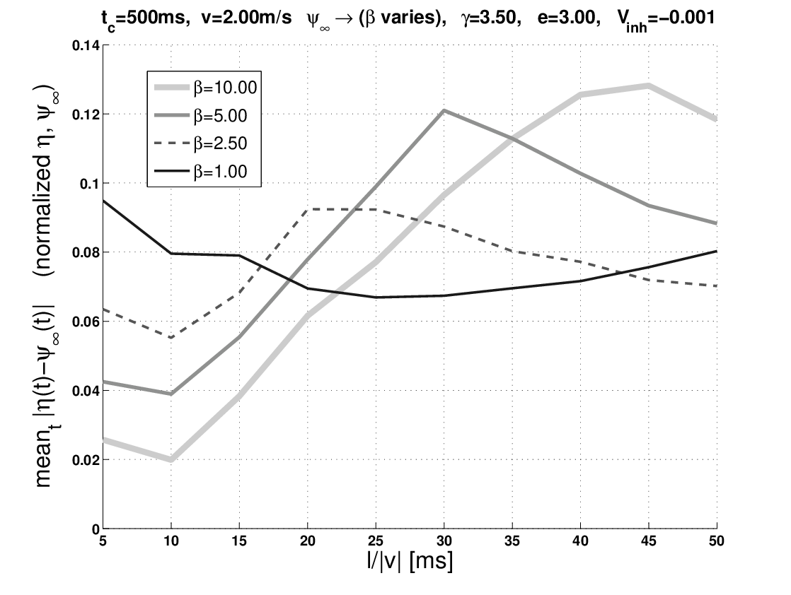
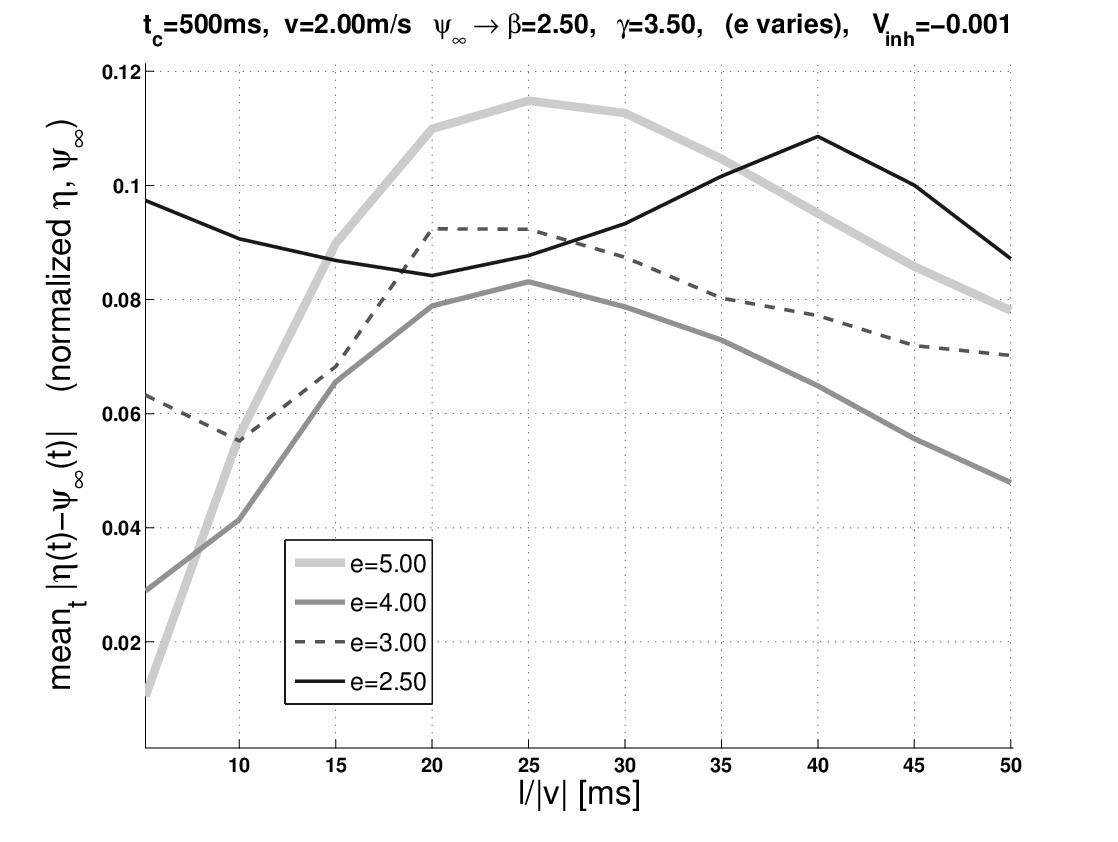
In order to get a notion about how well the shape of $\psi_{\infty}(t)$ matches $\eta(t)$, we computed time-averaged difference measures between normalized versions of both functions (details: figure 3 & 4). Bigger values of $\beta$ match $\eta$ better at smaller, but worse at bigger values of $l/|v|$ (figure 4a). Smaller $\beta$ cause less variation across $l/|v|$. As to variation of $e$, overall, curve shapes seem to be best aligned with $e=3$ to $e=4$ (figure 4b). Furthermore, better matches between $\psi_{\infty}(t)$ and $\eta(t)$ correspond to bigger values of $\gamma$ (figure 4c). And finally, $V_{inh}$ marches again to a different tune (data not shown). $V_{inh}=-0.1$ leads to the best agreement ($\approx 0.04$ across $l/|v|$) of all $V_{inh}$, quite different from the other considered values. For the rest, $\psi_{\infty}(t)$ and $\eta(t)$ align the same (all have maximum $0.094$), despite of covering different orders of magnitude with $V_{inh}=0,-0.001,-0.01$.
Decelerating approach. Hatsopoulos et al. [10] recorded DCMD activity in response to an approaching object which projected image edges on the retina moving at constant velocity: $\dot{\Theta}=const.$ implies $\Theta(t)=\Theta_{0}+\dot{\Theta}t$. This “linear approach” is perceived as if the object is getting increasingly slower. But what appears a relatively unnatural movement pattern serves as a test for the functions $\eta$ & $\psi_{\infty}$. Figure 5 illustrates that $\psi_{\infty}$ passes the test, and consistently predicts that activity sharply rises in the initial approach phase, and subsequently declines ($\eta$ passed this test already in the year 1995).
Spike traces. We re-sampled about $30$ curves obtained from LGMD recordings from a variety of publications, and fitted $\eta$ & $\psi_{\infty}$-functions. We cannot show the results here, but in terms of goodness of fit measures, both functions are in the same ballbark. Rather, figure 6a shows a representative example [30]. When $\alpha$ and $\beta$ are plotted against each other for five trials, we see a strong inverse correlation (figure 6b). Although five data points are by no means a firm statistical sample, the strong correlation could indicate that $\beta$ and $\alpha$ play similar roles in both functions. Biophysically, $\beta$ is the leakage conductance, which determines the (passive) membrane time constant $\tau_{m}\propto 1/\beta$ of the neuron. Voltage drops within $\tau_{m}$ to its $1/e$ part. Bigger values of $\beta$ mean shorter $\tau_{m}$ (i.e., “faster neurons”). Getting back to $\eta$, this would suggest $\alpha\propto\tau_{m}$, such that higher (absolute) values for $\alpha$ would possibly indicate a slower dynamic of the underlying processes.

Up to now, mainly two classes of LGMD models existed: The phenomenological $\eta$-function on the one hand, and computational models with neuronal layers presynaptic to the LGMD on the other (e.g. [25, 15]; real-world video sequences & robotics: e.g. [3, 14, 32, 2]). Computational models predict that LGMD response features originate from excitatory and inhibitory interactions in – and between – presynaptic neuronal layers. Put differently, non-linear operations are generated in the presynaptic network, and can be a function of many (model) parameters (e.g. synaptic weights, time constants, etc.). In contrast, the $\eta$-function assigns concrete nonlinear operations to the LGMD [7]. The $\eta$-function is accessible to mathematical analysis, whereas computational models have to be probed with videos or artificial stimulus sequences. The $\eta$-function is vague about biophysical parameters, whereas (good) computational models need to be precise at each (model) parameter value. The $\eta$-function establishes a clear link between physical stimulus attributes and LGMD activity: It postulates what is to be computed from the optical variables (OVs). But in computational models, such a clear understanding of LGMD inputs cannot always be expected: Presynaptic processing may strongly transform OVs.
The $\psi$ function thus represents an intermediate model class: It takes OVs as input, and connects them with biophysical parameters of the LGMD. For the neurophysiologist, the situation could hardly be any better. Psi implements the multiplicative operation of the $\eta$-function by shunting inhibition (equation 1: $V_{exc}\approx V_{rest}$ and $V_{inh}\approx V_{rest}$). The $\eta$-function fits $\psi$ very well according to our dynamical simulations (figure 1), and satisfactory by the approximate criterion of figure 4.
We can conclude that $\psi$ implements the $\eta$-function in biophysically plausible way. However, $\psi$ does neither explicitly specify $\eta$’s multiplicative operation, nor its exponential function $\exp(\cdot)$. Instead we have an interaction between shunting inhibition and a power law $(\cdot)^{e}$, with $e\approx 3$. So what about power laws in neurons?
Because of $e>1$, we have an expansive nonlinearity. Expansive power-law nonlinearities are well established in phenomenological models of simple cells of the primate visual cortex [1, 11]. Such models approximate a simple cell’s instantaneous firing rate $r$ from linear filtering of a stimulus (say $Y$) by $r\propto([Y]^{+})^{e}$, where $[\cdot]^{+}$ sets all negative values to zero and lets all positive pass. Although experimental evidence favors linear thresholding operations like $r\propto[Y-Y_{thres}]^{+}$, neuronal responses can behave according to power law functions if $Y$ includes stimulus-independent noise [19]. Given this evidence, the power-law function of the inhibitory input into $\psi$ could possibly be interpreted as a phenomenological description of presynaptic processes [2].

References

- [1] D.G. Albrecht and D.B. Hamilton, Striate cortex of monkey and cat: contrast response function, Journal of Neurophysiology 48 (1982), 217–237.
- [2] S. Bermudez i Badia, U. Bernardet, and P.F.M.J. Verschure, Non-linear neuronal responses as an emergent property of afferent networks: A case study of the locust lobula giant movemement detector, PLoS Computational Biology 6 (2010), no. 3, e1000701.
- [3] M. Blanchard, F.C. Rind, and F.M.J. Verschure, Collision avoidance using a model of locust LGMD neuron, Robotics and Autonomous Systems 30 (2000), 17–38.
- [4] D.F. Cooke and M.S.A. Graziano, Super-flinchers and nerves of steel: Defensive movements altered by chemical manipulation of a cortical motor area, Neuron 43 (2004), no. 4, 585–593.
- [5] L. Fogassi, V. Gallese, L. Fadiga, G. Luppino, M. Matelli, and G. Rizzolatti, Coding of peripersonal space in inferior premotor cortex (area f4), Journal of Neurophysiology 76 (1996), 141–157.
- [6] F. Gabbiani, I. Cohen, and G. Laurent, Time-dependent activation of feed-forward inhibition in a looming sensitive neuron, Journal of Neurophysiology 94 (2005), 2150–2161.
- [7] F. Gabbiani, H.G. Krapp, N. Hatsopolous, C.H. Mo, C. Koch, and G. Laurent, Multiplication and stimulus invariance in a looming-sensitive neuron, Journal of Physiology - Paris 98 (2004), 19–34.
- [8] F. Gabbiani, H.G. Krapp, C. Koch, and G. Laurent, Multiplicative computation in a visual neuron sensitive to looming, Nature 420 (2002), 320–324.
- [9] F. Gabbiani, H.G. Krapp, and G. Laurent, Computation of object approach by a wide-field, motion-sensitive neuron, Journal of Neuroscience 19 (1999), no. 3, 1122–1141.
- [10] N. Hatsopoulos, F. Gabbiani, and G. Laurent, Elementary computation of object approach by a wide-field visual neuron, Science 270 (1995), 1000–1003.
- [11] D.J. Heeger, Modeling simple-cell direction selectivity with normalized, half-squared, linear operators, Journal of Neurophysiology 70 (1993), 1885–1898.
- [12] A.L. Hodkin and A.F. Huxley, A quantitative description of membrane current and its application to conduction and excitation in nerve, Journal of Physiology 117 (1952), 500–544.
- [13] F. Hoyle, The black cloud, Pinguin Books, London, 1957.
- [14] M.S. Keil, E. Roca-Morena, and A. Rodríguez-Vázquez, A neural model of the locust visual system for detection of object approaches with real-world scenes, Proceedings of the Fourth IASTED International Conference (Marbella, Spain), vol. 5119, 6-8 September 2004, pp. 340–345.
- [15] M.S. Keil and A. Rodríguez-Vázquez, Towards a computational approach for collision avoidance with real-world scenes, Proceedings of SPIE: Bioengineered and Bioinspired Systems (Maspalomas, Gran Canaria, Canary Islands, Spain) (A. Rodríguez-Vázquez, D. Abbot, and R. Carmona, eds.), vol. 5119, SPIE - The International Society for Optical Engineering, 19-21 May 2003, pp. 285–296.
- [16] J.G. King, J.Y. Lettvin, and E.R. Gruberg, Selective, unilateral, reversible loss of behavioral responses to looming stimuli after injection of tetrodotoxin or cadmium chloride into the frog optic nerve, Brain Research 841 (1999), no. 1-2, 20–26.
- [17] C. Koch, Biophysics of computation: information processing in single neurons, Oxford University Press, New York, 1999.
- [18] D.N. Lee, A theory of visual control of braking based on information about time-to-collision, Perception 5 (1976), 437–459.
- [19] K.D. Miller and T.W. Troyer, Neural noise can explain expansive, power-law nonlinearities in neuronal response functions, Journal of Neurophysiology 87 (2002), 653–659.
- [20] Hideki Nakagawa and Kang Hongjian, Collision-sensitive neurons in the optic tectum of the bullfrog, rana catesbeiana, Journal of Neurophysiology 104 (2010), no. 5, 2487–2499.
- [21] M. O’Shea and C.H.F. Rowell, Projection from habituation by lateral inhibition, Nature 254 (1975), 53–55.
- [22] M. O’Shea and J.L.D. Williams, The anatomy and output connection of a locust visual interneurone: the lobula giant movement detector (lgmd) neurone, Journal of Comparative Physiology 91 (1974), 257–266.
- [23] S. Peron and F. Gabbiani, Spike frequency adaptation mediates looming stimulus selectivity, Nature Neuroscience 12 (2009), no. 3, 318–326.
- [24] F.C. Rind, A chemical synapse between two motion detecting neurones in the locust brain, Journal of Experimental Biology 110 (1984), 143–167.
- [25] F.C. Rind and D.I. Bramwell, Neural network based on the input organization of an identified neuron signaling implending collision, Journal of Neurophysiology 75 (1996), no. 3, 967–985.
- [26] F.C. Rind and P.J. Simmons, Orthopteran DCMD neuron: a reevaluation of responses to moving objects. I. Selective responses to approaching objects, Journal of Neurophysiology 68 (1992), no. 5, 1654–1666.
- [27] , Orthopteran DCMD neuron: a reevaluation of responses to moving objects. II. Critical cues for detecting approaching objects, Journal of Neurophysiology 68 (1992), no. 5, 1667–1682.
- [28] , Signaling of object approach by the dcmd neuron of the locust, Journal of Neurophysiology 77 (1997), 1029–1033.
- [29] , Reply, Trends in Neuroscience 22 (1999), no. 5, 438.
- [30] S.M. Roger, G.W.J. Harston, F. Kilburn-Toppin, T. Matheson, M. Burrows, F. Gabbiani, and H.G. Krapp, Spatiotemporal receptive field properties of a looming-sensitive neuron in solitarious and gregarious phases of desert locust, Journal of Neurophysiology 103 (2010), 779–792.
- [31] S.K. Rushton and J.P. Wann, Weighted combination of size and disparity: a computational model for timing ball catch, Nature Neuroscience 2 (1999), no. 2, 186–190.
- [32] Yue. S., Rind. F.C., M.S. Keil, J. Cuadri, and R. Stafford, A bio-inspired visual collision detection mechanism for cars: Optimisation of a model of a locust neuron to a novel environment, Neurocomputing 69 (2006), 1591–1598.
- [33] G.R. Schlotterer, Response of the locust descending movement detector neuron to rapidly approaching and withdrawing visual stimuli, Canadian Journal of Zoology 55 (1977), 1372–1376.
- [34] H. Sun and B.J. Frost, Computation of different optical variables of looming objects in pigeon nucleus rotundus neurons, Nature Neuroscience 1 (1998), no. 4, 296–303.
- [35] J.R. Tresilian, Visually timed action: time-out for ’tau’?, Trends in Cognitive Sciences 3 (1999), no. 8, 1999.
- [36] Y. Wang and B.J. Frost, Time to collision is signalled by neurons in the nucleus rotundus of pigeons, Nature 356 (1992), 236–238.
- [37] J.P. Wann, Anticipating arrival: is the tau-margin a specious theory?, Journal of Experimental Psychology and Human Perceptual Performance 22 (1979), 1031–1048.
- [38] M. Wicklein and N.J. Strausfeld, Organization and significance of neurons that detect change of visual depth in the hawk moth manduca sexta, The Journal of Comparative Neurology 424 (2000), no. 2, 356–376.