Improved Parameterization of K+ Production in p-Be Collisions at Low Energy
Using Feynman Scaling
Abstract
This paper describes an improved parameterization for proton-beryllium production of secondary mesons for experiments with primary proton beams from 8.89 to 24 GeV/c. The parameterization is based on Feynman scaling in which the invariant cross section is described as a function of and . This method is theoretically motivated and provides a better description of the energy dependence of kaon production at low beam energies than other parameterizations such as the commonly used “Modified Sanford-Wang” model. This Feynman scaling parameterization has been used for the simulation of the neutrino flux from the Booster Neutrino Beam at Fermilab and has been shown to agree with the neutrino interaction data from the SciBooNE experiment. This parameterization will also be useful for future neutrino experiments with low primary beam energies, such as those planned for the Project X accelerator.
pacs
13.25.Es,13.87.CeI Introduction
This paper describes a parameterization for inclusive production of secondary mesons in proton-beryllium collisions,
| (1) |
for experiments with low primary proton beam energies ranging in kinetic energy from below 9 to 24 GeV. The parameterization is based on Feynman scaling(F-S) [1], in which the invariant cross section is described as a function of transverse momentum, , and a scaling variable, . Various scaling parameterizations are known to describe data well above 20 GeV [2, 3]. In this paper, we show that the F-S form describes data down to 8.89 GeV/c beam momentum. This result provides an alternative model to the traditional “Modified Sanford-Wang” [4, 5] parameterization used to describe secondary production at low primary proton beam momentum. The results from this F-S analysis have been used in the neutrino flux parameterization of the Booster Neutrino Beam (BNB) at Fermilab and has been checked against measurements by the SciBooNE experiment [6]. This parameterization will be useful for future neutrino experiments using low primary proton beam energies.

The primary motivation for this work was the simulation of neutrinos in the BNB line. This line provides neutrinos for the MiniBooNE [7] and SciBooNE [6] experiments, as well as possible future experiments, including the upcoming MicroBooNE [8] experiment. In this beam line, protons with 8 GeV kinetic energy are directed onto a 1.8 interaction length beryllium target. The charged pions and kaons which are produced are focused by a magnetic horn into a 50 m decay region, where they subsequently decay to produce neutrinos. The average energy of () that decay to neutrinos in the MiniBooNE detector acceptance is 1.89 (2.66) GeV. Therefore 37.6% (92.1%) of the particles decay before the end of the 50 m long decay region. The most relevant decay modes for MiniBooNE are , , which produce 99.4% of the neutrino beam, and , , , and , which produce the remaining 0.6%.
Figure 1 shows the predicted flux for the BNB line at the MiniBooNE detector. While the flux is predominately due to decay, the decay is the dominant source above 2 GeV. The flux from kaon decay contributes one of the important backgrounds for neutrino oscillation searches looking for appearance. In addition, the kaon neutrino flux provides an interesting source of high energy events for experiments on the BNB line for studying neutrino cross sections. Therefore, it is important for the BNB line experiments to have a good first-principles prediction of production.
A first-principles prediction for production is obtained from fitting data from secondary production experiments with primary beam momentum ranging from 8.89 to 24 GeV/c. Nine data sets are considered, but only seven are used in the fit as it will be explained in Section III. Because these data are taken at a range of beam energies, the data must be fit to a parameterization including changes with beam momentum in order to scale the result to the 8.89 GeV/c of the BNB line momentum.
I.1 Feynman Scaling Formalism
Over the past several decades, many experiments have made measurements of particle production by protons of various energies on many different nuclear targets. These data have been used to study the phenomenology of particle production and have led to several scaling laws and quark counting rules. For inclusive particle production, Feynman put forward a theoretical model [1] where the invariant cross section is only a function of and . The invariant cross section is related to the commonly used differential cross section by:
| (2) |
Defining
| (3) |
this leads to:
| (4) |
is a factor and is the F-S function that depends on and . The quantity , which appears in the denominator of the definition of , depends upon the particle being produced and is derived from the exclusive channels given in Table 1.
| Produced | Exclusive | MX | E | |
|---|---|---|---|---|
| Hadron | Reaction | (GeV/c | (GeV) | GeV |
| pn | 1.878 | 2.018 | 1.233 | |
| pp | 2.016 | 2.156 | 1.54 | |
| pp | 1.876 | 2.011 | 1.218 | |
| 2.053 | 2.547 | 2.52 | ||
| pp | 2.37 | 2.864 | 3.434 | |
| p | 2.13 | 2.628 | 2.743 |
Feynman scaling has been demonstrated for secondary meson production at primary beam energies above 15 to 20 GeV [9, 2, 3]; this paper demonstrates the validity of F-S at lower primary beam energies for production. One might expect F-S to be a better parameterization of production than the “Modified Sanford-Wang” formalism for two reasons. First, the F-S parameterization properly accounts for the kinematic effects of the large kaon mass where even at , the outgoing kaon can have a significant laboratory momentum. Second, the functional form of the parameterization typically has peak production at . This is in contrast to the “Modified Sanford-Wang” formalism, where the production rate continues to grow as becomes more negative.
I.2 Feynman Scaling Parameterization for the Particle Production Cross Section
The Feynman model can be used to describe the expected and dependence using theoretically inspired functions for these dependences. For the dependence, a parameterization proportional to or has the properties consistent with a flat rapidity plateau around . The expectation of a limited range is provided by including exponential moderating factors for powers of .
Using this guidance, a F-S parameterization has been developed to describe kaon production. In order to allow some coupling between the and distribution an additional exponential factor has been added that uses the product, . The ’s are the seven coefficients of the F-S function. The kinematic threshold constraint for production is imposed by setting equal to zero for .
Including these factors, the final parameterization has the form:
| (5) |
I.3 The “Modified Sanford-Wang” Parameterization
| (6) |
This functional form allows for some phenomenological parameterization of the variations associated with beam energy and process thresholds. As noted in one of the initial Sanford-Wang papers [4, 5], the coefficients for production are approximately given by: and the term is negligible. With these substitutions, the formula shows a close although not perfect relationship with F-S (see Eq. 5)
| (7) |
where
| (8) |
and
| (9) |
Therefore, the S-W fits to the K+ data will show only approximate consistency with F-S. At low beam energy, produced particle mass effects can become important. Table 1 gives the minimum mass channels, their invariant mass, and the beam energy threshold for different particle production processes. In the S-W formula, the parameter is included to approximately provide the kinematic limit for produced particle momentum. Investigations of the exact kinematic threshold for production show that the maximum is approximately equal to where varies from 1.7 to 2.2 GeV as goes from 0 to 0.3 rad. One would therefore expect that would take on values similar to . On the other hand, the factor introduces violations of the scaling behavior away from this limiting region.
| K+Data | Ref. | (GeV/c) | PK(GeV/c) | (rad) | (GeV/c) | ||
|---|---|---|---|---|---|---|---|
| Abbott | [10] | 14.6 | 10% | ||||
| Aleshin | [11] | 9.5 | 10% | ||||
| Allaby | [12] | 19.2 | 15% | ||||
| Dekkers | [13] | 18.8 , 23.1 | 20% | ||||
| Eichten | [14] | 24.0 | 20% | ||||
| Lundy | [15] | 13.4 | 20% | ||||
| Marmer | [16] | 12.3 | 20% | ||||
| Piroue | [17] | 2.74 | 20% | ||||
| Vorontsov | [18] | 10.1 | 25% |
An additional problem with the S-W parameterization is that most of the function parameters () will be effectively fixed by the scaling constraints, and this will be limiting the flexibility of the function to match the and behavior. The parameter , for example, should be close to unity to provide the conversion from invariant to differential cross section. The parameter needs to be approximately equal to 2.0 GeV to provide the maximum dependence, and the parameters and should be equal in order to preserve a basic dependence. Thus, the S-W parameterization has very little flexibility to fit the data distributions over the full kinematic range and therefore a formalism like Feynman scaling is required. In many of the following plots, we will compare prediction results coming from S-W and F-S parameterizations.
II External Data Sets and Kinematic Coverage
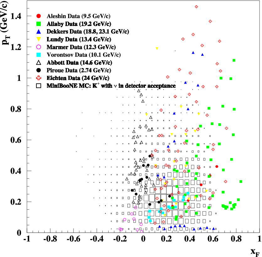
Several production measurements have been made for beam momentum less than 25 GeV/c and are reported in Table 2. Those experiments, except for Piroue, have beam momenta higher than the BNB value of 8.89 GeV/c although some of them such as Aleshin and Vorontsov are fairly close to the BNB beam momentum. The kaons that produce neutrinos in MiniBooNE span the kinematic region with -0.10.5 and 0.050.5 as shown in Figure 2, which is nicely covered by the experimental data sets listed in Table 2. Of course, we are using the assumption that one can extrapolate these higher beam momentum data to the BNB energy value using a parameterization such as F-S. Thus, the first question to be answered is whether the data appears to follow these scaling parameterizations.
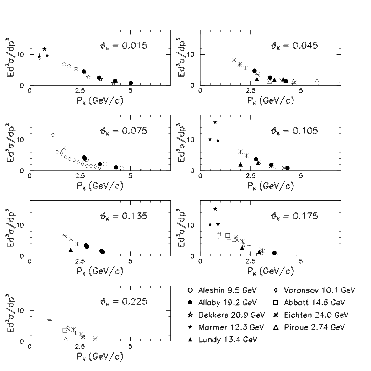
The F-S hypothesis says that the invariant cross section should only depend on and . This hypothesis can further be tested by scaling all the data to a common beam momentum and checked by the behavior of the invariant cross section against the scaled value of and . Figure 3 shows the invariant cross section for scaled kaon momentum and angle bins using the F-S assumption. For this plot, the data from each data set is converted first to and and then scaled to and for a 8.89 GeV/c beam momentum. For example, given a cross section point at =20 GeV/c with a given and , one can calculate the and for this point. One can then find the equivalent and that would have the same and at =8.89 GeV/c. As seen from the plots, the data appears to obey the scaling hypothesis reasonably well except for the Lundy, Piroue, and Vorontsov data sets. Due to the disagreements of the Lundy and Piroue data, these data sets are not included in the fits described below. The Vorontsov data appears to agree in shape with the other data sets but has an anomalous normalization. Data sets not included in the fits are not discarded. They are compared separately to the fit results, as explained below.
III Feynman Scaling and Sanford-Wang Model Fits to the K+ External Data Sets
Under the assumption that the experimental data follow the Feynman or S-W scaling models, we can determine a parameterization that best fits these data sets. The various production data sets are used as input to a fit for the scaling function parameters that best describe the data. The fit uses a minimization technique using Minuit [19] to perform the numerical minimization. Each experiment is allowed to have an independent normalization parameter that is constrained by the published normalization uncertainty. The fit minimizes the following function for an experiment :
| (10) |
where is the (,) bin index, is the scaling function prediction evaluated at the given , is the measurement at a given , is the data error for measurement , is the scaling factor to bring the is the normalization factor for experiment , is the normalization uncertainty for experiment , and d.o.f. indicates degree of freedom. The total for external data sets is then the sum over the experiments of the individual values,
| (11) |
The is minimized in order to obtain the best values and uncertainties for the parameterization coefficients , given in Eq. 5 (or 6, and for the normalization factors ). The uncertainties on the fit values at 1 are determined from a change with respect to and the fit also yields a covariance matrix that can be used to propagate correlated errors associated with the parameterization of the cross section.
A F-S fit to all the experimental data sets with 0.06.0 gives a /d.o.f. equal to 4.03 with large contributions from data with 1.2 GeV/c and 5.5 GeV/c. Therefore for the final scaling fits, the points with the larger pull terms, defined as (), have been eliminated by only using data with 1.25.5.
The 1.2 GeV/c cut effectively removes data at negative where the nuclear environment starts to play an important role. This cut also eliminates all the Marmer data points.
With all of these requirements, the /d.o.f. for the F-S fit is reduced to 2.28. The uncertainties for the fitted cross section need to be corrected for this /d.o.f., which is larger than 1.0. This is accomplished by scaling up the errors of each of the data points by before doing the fit. Figure 4 shows the pull terms for the seven parameter F-S fit where the errors have been scaled up by this 1.51.

A S-W fit to all the experimental data has been performed as well. To be able to directly compare the S-W with the F-S fit we have included in the S-W fit only data with 1.25.5. The /d.o.f. for the S-W fit is equal to 6.05.
| Feynman Scaling | 1.25.5 | ||
|---|---|---|---|
| Fit | Value | Error | |
| c1 | 11.70 | 1.05 | |
| c2 | 0.88 | 0.13 | |
| c3 | 4.77 | 0.09 | |
| c4 | 1.51 | 0.06 | |
| c5 | 2.21 | 0.12 | |
| c6 | 2.17 | 0.43 | |
| c7 | 1.51 | 0.40 | Input Error |
| Aleshin | 1.09 | 0.07 | 0.10 |
| Allaby | 1.04 | 0.07 | 0.15 |
| Dekkers | 0.84 | 0.06 | 0.20 |
| Vorontsov | 0.53 | 0.04 | 5.00 |
| Abbott | 0.76 | 0.07 | 0.15 |
| Eichten | 1.00 | 0.07 | 0.15 |
| /d.o.f. (no ) | 2.28 | () | |
| Modified S-W | 1.25.5 | ||
|---|---|---|---|
| Fit | Value | Error | |
| c1 | 14.89 | 1.89 | |
| c2 | 0.91 | 0.13 | |
| c3 | 12.80 | 7.46 | |
| c4 | 2.08 | 0.35 | |
| c5 | 2.65 | 0.50 | |
| c6 | 4.61 | 0.10 | |
| c7 | 0.26 | 0.01 | |
| c8 | 10.63 | 7.06 | |
| c9 | 2.04 | 0.01 | Input Error |
| Aleshin | 1.02 | 0.09 | 0.10 |
| Allaby | 0.74 | 0.09 | 0.15 |
| Dekkers | 0.57 | 0.08 | 0.20 |
| Vorontsov | 0.42 | 0.04 | 5.00 |
| Abbott | 1.38 | 0.11 | 0.15 |
| Eichten | 0.59 | 0.08 | 0.15 |
| /df (no ) | 6.05 | () | |
IV Comparison of Feynman Scaling to Sanford Wang Results and Neutrino Predictions
Tables 3 and 4 report the final fit values for the coefficients and the normalization factors for the F-S and S-W parameterizations respectively. Figures 5 and 6 show the fit function curves for the F-S and S-W parameterizations as compared to the data. The fits are stable with respect to parameter starting values and yield positive definite covariance matrices. The error bands in Figures 5 and 6 are determined by propagating the covariance matrix for the parameters to the invariant cross section errors.
As seen from the plots, the F-S function gives a very good description of the data over the full kaon momentum range used in the fit and has a reasonable /d.o.f. = 2.3. Below 1.2 GeV/c, the F-S prediction has some disagreement with a few the of the Marmer (not included in the fit) and Abbott data points but in general is also fitting that well in that region. The normalization factors for the F-S fits are within of the quoted experimental error except for the Vorontsov data (see Table 3). As mentioned above, the Vorontsov data shows a systematically low normalization with respect the other sets of scaled data. Therefore, for all the scaling fits, the Vorontsov data has only been used for shape information by giving the normalization a large uncertainty (500%).
In contrast, the S-W final fit parameterization has rather large discrepancies with the data in almost all regions and has a much larger /d.o.f. = 6.05. Additionally, the normalization factors given in Table 4 are very much outside of the quoted experimental errors and, for example, the factors for Eichten and Allaby differ from 1.0 by 2 to 3.


Tables 5 and 6 list the differential cross sections for several different kinematic points for kaon production. The uncertainties are obtained by propagating the covariance matrix for the coefficients into the scaling function. The first three points in Table 5 and 6 correspond to the mean kaon production points that produce electron neutrino of 0.35, 0.65, and 0.95 GeV in MiniBooNE. The fourth point corresponds to the kaon kinematics that produce average energy neutrinos from all kaon decays (called the “kaon sweet spot”), and the fifth point is associated with the mean kaon kinematics for the highest energy kaon-decay muon neutrinos observed in MiniBooNE. As seen from Table 5 and 6 , the two parameterizations give much different results for the cross section values and uncertainties with the F-S fit giving a larger value by a factor 2 for the lowest energy neutrino bin at 0.35 GeV. The source of the this discrepancy is a large drop in the invariant cross section of the S-W parameterization at large angles.
| (GeV/c) | (rad) | (mb) | |
|---|---|---|---|
| GeV | 1.52 | 0.213 | 9.37 0.73 (7.8%) |
| GeV | 2.07 | 0.127 | 10.69 0.75 (7.0%) |
| GeV | 2.45 | 0.103 | 10.22 0.71 (6.9%) |
| Kaon Sweet Spot | 2.80 | 0.106 | 8.67 0.60 (6.9%) |
| HE Events | 4.30 | 0.055 | 4.73 0.33 (7.0%) |
| (GeV/c) | (rad) | (mb) | |
|---|---|---|---|
| GeV | 1.52 | 0.213 | 4.25 0.77 (18%) |
| GeV | 2.07 | 0.127 | 8.99 1.34 (15%) |
| GeV | 2.45 | 0.103 | 9.91 1.43 (14%) |
| Kaon Sweet Spot | 2.80 | 0.106 | 7.73 1.13 (15%) |
| HE Events | 4.30 | 0.055 | 5.24 0.84 (16%) |
The predictions for the size and kinematic dependence of the invariant differential cross section as function of momentum are quite different for the F-S and S-W parameterizations as shown in Figure 7, especially for low value of the momentum.
To illustrate the difference between the F-S and the S-W predictions, we have used an analytic simulation of the BNB neutrino beam line designed for the MiniBooNE experiment (described in Reference [20]). Table 7 gives the comparison of the predicted event rate from using the above F-S and S-W production parameterizations as calculated using this BNB simulation.

| Feynman Scaling Fit | Sanford-Wang Fit | |||||
| Angular Bins(rad) | All Eν(GeV) | 1 GeV | 2 GeV | All (GeV) | 1 GeV | 2 GeV |
| 0.015 | 36.7 | 2.6 | 18.0 | 43.4 | 3.3 | 19.3 |
| 0.045 | 92.5 | 8.4 | 35.9 | 111.0 | 12.0 | 35.9 |
| 0.075 | 110.5 | 13.7 | 27.0 | 141.3 | 22.6 | 26.5 |
| 0.105 | 96.8 | 17.2 | 4.4 | 138.3 | 32.6 | 4.1 |
| 0.135 | 59.1 | 21.8 | 0.0 | 100.5 | 45.8 | 0.0 |
| 0.175 | 39.4 | 32.4 | 0.0 | 83.7 | 73.9 | 0.0 |
| 0.225 | 21.9 | 21.9 | 0.0 | 56.8 | 56.8 | 0.0 |
| Total | 476.6 | 137.9 | 85.3 | 731.2 | 303.4 | 85.9 |
V High energy parameterization
The hypothesis of F-S has also been verified to hold with different parameterizations over a wide range of primary proton beam energies (from 24 GeV to 450 GeV). In Bonesini et al. [2] data at higher proton energies has been empirically parameterized as a function of the transverse momentum () and the scaling variable where is the energy of the particle in center-of-mass frame. The choice of these variables for the description of the invariant cross section (radial scaling) is motivated again by an assumed scaling behavior of the invariant cross section. The radial scaling variable is approximately equal to the F-S variable at high energy and has the property of never taking on a negative value. (A detailed comparison of radial scaling and F-S can be found in [21, 3], where the authors compare different models with the production data at different energies down to about 24 GeV.)
Bonesini et al.[2] has obtained an empirical parameterization based on radial scaling fits to data collected with 400 GeV/c and 450 GeV/c protons incident on a Be target. The results from this parameterization are compared in Figure 7 to the predictions of F-S and S-W models at a proton momentum of 8.89 GeV/c. As seen from Figure 7, this radial scaling model underestimates production at a beam momentum of 8.89 GeV/c by more than a factor of two even though the parameterization describes well the high proton momentum data (24 GeV/c) [2].
VI The SciBooNE Measurements
The SciBooNE collaboration has reported a measurement [22] for production in the BNB with respect to the Monte Carlo (MC) beam simulation. The SciBooNE experiment collected data in 2007 and 2008 with neutrino ( protons on target (POT)) and antineutrino ( POT) beams in the FNAL BNB line. The SciBooNE detector is located 100 m downstream from the neutrino production target. The flux-averaged mean neutrino energy is 0.7 GeV in neutrino running mode and 0.6 GeV in antineutrino running mode
The SciBooNE detector consists of three detector components; SciBar, Electromagnetic Calorimeter (EC) and Muon Range Detector (MRD). SciBar is a fully active and fine grained scintillator detector that consists of 14,336 bars arranged in vertical and horizontal planes. SciBar is capable of detecting all charged particles and performing dE/dx-based particle identification. The EC is located downstream of SciBar. The detector is a ÒspaghettiÓ calorimeter with thickness of 11 radiation lengths and is used to measure and the intrinsic component of the neutrino beam. The MRD is located downstream of the EC in order to measure the momentum of muons up to 1.2 GeV/c with range. It consists of 2-inch thick iron plates sandwiched between layers of plastic scintillator planes.
In the SciBooNE experiment, particle production is simulated using the methods described in Ref. [20]. The production of is simulated using the F-S formalism as described in Section I.1 with the coefficients reported in Table 3. The predicted double differential cross section at the mean momentum and angle for kaons which produce neutrinos in SciBooNE ( = 3.87 GeV/c and = 0.06 rad) is
| (12) |
The error on the double differential cross section prediction using the F-S parametrization at the SciBooNE and is 7%. The SciBooNE and MiniBooNE collaboration have adopted a conservative error of 40%. This larger error was chosen because of the uncertainties in extrapolating the prediction data from high to low proton beam energy using the F-S and S-W models as explained in References [22, 20].
VI.1 SciBooNE Production Measurement
The SciBooNE data can be used as an additional constraint in fits to production cross sections. In SciBooNE, neutrinos from decay are selected using high energy interactions within the volume of the SciBar detector. The high-energy selection is accomplished by isolating charged current interactions that produce a muon that crosses the entire MRD. This sample is further divided into three sub-samples based on whether 1, 2, or 3 reconstructed SciBar tracks are identified at the neutrino interaction vertex in the SciBar detector. Since the reconstruction of the energy of the muon is not possible because the muon exits the MRD detector, the reconstructed muon angle relative to beam axis is used as the primary kinematic variable to separate neutrinos from pion and kaon decay. The values for for neutrino, antineutrino, and combined data mode running are given in Table 8 along with the mean energy and angles for the corresponding samples. The F-S and S-W prediction values are obtained using the parametrizations described in Section I.1 and I.3 along with the parameters listed in Table 3 and 4.
| (GeV) | (rad) | ||
| (mb/(GeV/c sr) | |||
| -mode | 3.810.03 | 0.070.01 | 5.770.83 |
| -mode | 4.290.06 | 0.030.01 | 3.181.94 |
| + -mode | 3.900.03 | 0.060.01 | 5.340.76 |
| F-S prediction | 3.90 | 0.06 | 6.300.44(7%) |
| S-W prediction | 3.90 | 0.06 | 6.841.09(16%) |
The momentum versus angle distribution for the 2-track SciBar sample in the simulation is shown in Figure 8.


Figure 8 shows the kinematics of the selected events in SciBooNE, while Figure 9 shows the kinematical region as function of angle and momentum for mesons that produce events in MiniBooNE.

The SciBooNE measurement is a direct test of the extrapolation of parameterizations found from higher beam energies to the MiniBooNE beam energy. The predictions for the double differential cross section for the F-S and S-W models are reported in Table 8 and shows a good agreement with the SciBooNE measurement, a better agreement is found in the case of the F-S parametrization.
The SciBooNE production measurements can also be added to the F-S fit as additional external data using the following procedure. First we retrieve all the SciBooNE MC events with their and for the neutrino and antineutrino sample. Then we calculate the following quantities:
| (13) | |||||
| (14) |
These quantities are then used at each fit step to build a pull term, defined in Eq. 15, to be added to the of the fit.
| (15) |
Each data point in and is reweighted using the double differential cross section value for the current set of
coefficient of Eq. 5 computed at each step of the Minuit fit. The set of coefficient used in the MC is labeled as , the values of these coefficients is listed in Table 3. The and in the Eq. 15 are the values of the SciBooNE production measurement and error (see Table 8), respectively.
Two separate pull terms are added to the fit corresponding to the SciBooNE neutrino and antineutrino production measurements.
The results of scaling function fit to all experiments with 1.25.5 GeV/c, including the SciBooNE data, are given in Table 9. The covariance matrix is given in Table 10 and the correlation matrix is presented in Figure 10.
Table 11 lists the differential cross section for the kaon production at the various kaon kinematic points. The uncertainties are obtained as described in Section IV.
| Scaling Fits | 1.25.5 | ||
|---|---|---|---|
| Value | Error | ||
| c1 | 11.29 | 0.93 | |
| c2 | 0.87 | 0.13 | |
| c3 | 4.75 | 0.09 | |
| c4 | 1.51 | 0.06 | |
| c5 | 2.21 | 0.12 | |
| c6 | 2.17 | 0.43 | |
| c7 | 1.51 | 0.40 | Input Error |
| Aleshin | 1.12 | 0.07 | 0.10 |
| Allaby | 1.07 | 0.06 | 0.15 |
| Dekkers | 0.87 | 0.06 | 0.20 |
| Vorontsov | 0.55 | 0.04 | 5.00 |
| Abbott | 0.79 | 0.07 | 0.15 |
| Eichten | 1.03 | 0.06 | 0.15 |
| /df (no ) | 2.28 | () | |
| c1 | c2 | c3 | c4 | c5 | c6 | c7 | |
|---|---|---|---|---|---|---|---|
| c1 | 0.84 | 0.48E-01 | 0.39E-02 | -0.32E-01 | -0.36E-01 | 0.12 | 0.69E-01 |
| c2 | 0.48E-01 | 0.16E-01 | 0.14E-02 | -0.15E-02 | -0.13E-01 | 0.32E-01 | 0.22E-01 |
| c3 | 0.39E-02 | 0.14E-02 | 0.73E-02 | 0.20E-02 | 0.19E-02 | 0.14E-01 | -0.29E-02 |
| c4 | -0.32E-01 | -0.15E-02 | 0.20E-02 | 0.34E-02 | 0.20E-02 | -0.39E-02 | -0.60E-02 |
| c5 | -0.36E-01 | -0.13E-01 | 0.19E-02 | 0.20E-02 | 0.15E-01 | -0.15E-01 | -0.24E-01 |
| c6 | 0.12 | 0.32E-01 | 0.14E-01 | -0.39E-02 | -0.15E-01 | 0.18 | 0.12 |
| c7 | 0.69E-01 | 0.22E-01 | -0.29E-02 | -0.60E-02 | -0.24E-01 | 0.12 | 0.15 |
| (GeV/c) | (rad) | (mb) | |
|---|---|---|---|
| GeV | 1.52 | 0.213 | 9.05 0.62 (6.9%) |
| GeV | 2.07 | 0.127 | 10.32 0.62 (6.0%) |
| GeV | 2.45 | 0.103 | 9.87 0.58 (5.9%) |
| Kaon Sweet Spot | 2.80 | 0.106 | 8.37 0.49 (5.9%) |
| HE Events | 4.30 | 0.055 | 4.57 0.27 (5.9%) |
Table 10 gives the covariance matrix for the baseline scaling fit using kaon production data with 1.25.5 GeV/c. The correlation matrix is basically made of two blocks, one associated with the through parameters and one associated with the experimental normalization factors. The only coupling of these two sets is through which has significant correlations with the normalization factors. This is expected since the parameter sets the normalization of the scaling function and should be determined by the data normalizations.

The terms of the covariance matrix from the F-S fit that includes the SciBooNE production measurement include the factor 1.51 for the data set errors rescaling.
The relative uncertainties on the predicted double differential cross section by the F-S fit as function of angle and momentum decrease including the SciBooNE measurement as shown in Figures 11 and 12.


The SciBooNE measurement confirms the validity of the F-S parametrization and including the SciBooNe measurement as an additional experimental data to the Feynman Scaling fit contributes in improving both the error uncertainty on the parametrization coefficients and in lowering the total uncertainty in the predicted production at 8.89 GeV/c proton momentum.
VI.2 SciBooNE Rate Measurement
In addition to a measurement of production, the SciBooNE collaboration has also published a measurement of the observed to MC predicted ratio for produced neutrinos and antineutrinos interacting in the SciBar detector. The results are summarized in Table 12. The SciBooNE rate is the product of the production and neutrino cross section on carbon as explained in Ref. [22]. Since this result also includes the neutrino interaction cross section, it cannot be directly compared with the other experimental data presented in Table 2. This constraint not only covers the neutrino flux from decay but also constrains the neutrino interaction cross section because the two targets are composed of similar material. It should be noted that this analysis is a specific application to MiniBooNE and is not a general result. Nevertheless, the SciBooNE neutrino rate measurement can be directly applied to MiniBooNE analysis as a constraint on the electron and muon neutrinos from decay. Electron neutrinos from decays are one of the important background in the to oscillation search. Understanding this background will result in a reduction of the systematic uncertainty in the MiniBooNE oscillation analysis.
| Combined | |||
|---|---|---|---|
| -mode | -mode | + mode | |
| Rate | 0.940.050.11 | 0.540.090.30 | 0.880.040.10 |
This SciBooNE rate measurement has been included in a version of the F-S fit and the best fit results for the parameters including the normalization for the data sets is reported in Table 13. The covariance matrix is reported in Table 14 and correlation matrix is displayed in Figure 13. Table 15 lists the differential cross section values for kaon production at several kinematic points.
| Scaling Fits | |||
|---|---|---|---|
| Value | Error | ||
| c1 | 11.37 | 0.93 | |
| c2 | 0.87 | 0.13 | |
| c3 | 4.75 | 0.09 | |
| c4 | 1.51 | 0.06 | |
| c5 | 2.21 | 0.12 | |
| c6 | 2.17 | 0.43 | |
| c7 | 1.51 | 0.40 | Input Error |
| Aleshin | 1.11 | 0.07 | 0.10 |
| Allaby | 1.07 | 0.06 | 0.15 |
| Dekkers | 0.87 | 0.06 | 0.20 |
| Vorontsov | 0.54 | 0.04 | 5.00 |
| Abbott | 0.78 | 0.07 | 0.15 |
| Eichten | 1.03 | 0.06 | 0.15 |
| /d.o.f. (no ) | 2.28 | (d.o.f. = 119) | |
| c1 | c2 | c3 | c4 | c5 | c6 | c7 | |
|---|---|---|---|---|---|---|---|
| c1 | 0.84 | 0.47E-01 | 0.39E-02 | -0.31E-01 | -0.36E-01 | 0.12 | 0.69E-01 |
| c2 | 0.47E-01 | 0.16E-01 | 0.14E-02 | -0.14E-02 | -0.13E-01 | 0.32E-01 | 0.22E-01 |
| c3 | 0.40E-02 | 0.14E-02 | 0.73E-02 | 0.20E-02 | 0.19E-02 | 0.14E-01 | -0.33E-02 |
| c4 | -0.31E-01 | -0.14E-02 | 0.20E-02 | 0.34E-02 | 0.20E-02 | -0.38E-02 | -0.61E-02 |
| c5 | -0.36E-01 | -0.13E-01 | 0.19E-02 | 0.20E-02 | 0.15E-01 | -0.15E-01 | -0.24E-01 |
| c6 | 0.12 | 0.32E-01 | 0.14E-01 | -0.38E-02 | -0.15E-01 | 0.18 | 0.12 |
| c7 | 0.69E-01 | 0.22E-01 | -0.33E-02 | -0.61E-02 | -0.24E-01 | 0.12 | 0.16 |
| (GeV/c) | (rad) | (mb) | |
|---|---|---|---|
| GeV | 1.52 | 0.213 | 9.12 0.62 (6.8%) |
| GeV | 2.07 | 0.127 | 10.39 0.62 (6.0%) |
| GeV | 2.45 | 0.103 | 9.94 0.58 (5.8%) |
| Kaon Sweet Spot | 2.80 | 0.106 | 8.43 0.49 (5.8%) |
| HE Events | 4.30 | 0.055 | 4.60 0.27 (5.8%) |

In order to apply the SciBooNE constraint to the MiniBooNE neutrino event prediction, one needs to consider the kinematic regions that contribute to the two samples.
Figure 9 shows that the kinematic region of mesons that produce background events in MiniBooNE and Figure 8 shows the regions that contributes to the SciBooNE rate measurement. While there is a large overlap between the SciBooNE and MiniBooNE regions, the MiniBooNE region extends to somewhat lower momenta. Using MC studies combined with the covariance matrix associated with F-S fit, we have quantified the increased uncertainty associated with extrapolating the SciBooNE measurement to the lower MiniBooNE region and found that the error on the constrained electron neutrino interaction rate should be increased by a factor of 1.5. This increases the uncertainty for the MiniBooNE electron neutrino event rate prediction from the measured SciBooNE uncertainty of 12% (as reported in Table 12) to a total error of 18%. (The associated covariance matrix given in Table 14 should also have all of the elements multiplied by ) After applying the new SciBooNE constraint, the MiniBooNE prediction for electron neutrinos from decay is reduced by only 3% but the uncertainty is reduced significantly by a factor of three from previous estimates because both the rate and cross section uncertainty is reduced [23].
VII Summary and Conclusions
The F-S parameterization given in Eq. 5 has a theoretically motivated form that takes into account low beam momentum production thresholds from exclusive channels in contrast to many other models. For example, the S-W parameterization does not have the proper scaling properties or expected behavior for the regions. Also, extrapolations using data at much higher beam momentum appear to have difficulty describing lower momentum production measurements.
The F-S parameterization describes the production data well for beam momentum in the range of 8.89 to 24 GeV/c. Fits involving different experimental data sets have been performed and show good agreement with the experimental data as shown in Figure 5 where the data have been scaled by the normalization factors given in Table 3. The normalization values (except for the Vorontsov data) are in good agreement within the 10% to 20% uncertainties quoted by the experiments.
The F-S fits including the full covariance matrix can be used to predict production for low beam momentum neutrino experiments such as the BNB at 8.89 GeV/c. The overall uncertainty from the fit is about 7% and is consistent with the combination of the experiments with 15% uncertainties. The fits also give the dependence on produced kinematics in angle and momentum, which is important for accurate neutrino flux predications using magnetic horn focusing devices.
A cross check of the F-S parameterization using neutrino data from the SciBooNE collaboration measurement reported in Ref. [22] confirms the accuracy of the model at low primary beam momenta and its validity as a better representation of production with respect to the S-W model. The F-S parameterization derived from the low energy kaon production experiments including this SciBooNE production constraint should therefore be a good representation of production for low energy neutrino beam simulations. We, therefore, suggest that the parameters shown in Table 9 be used along with the covariance given in Table 10.
We wish to acknowledge the MiniBooNE and SciBooNE Collaboration for the use of their neutrino simulation programs and the National Science Foundation for the support.
References
- [1] R. P. Feynman, Phys. Rev. Lett. 23, 1415 (1969).
- [2] M. Bonesini, A. Marchionni, F. Pietropaolo, and T. Tabarelli de Fatis, Eur. Phys. J. C20, 13 (2001), eprint hep-ph/0101163.
- [3] J. W. Norbury, The Astrophysical Journal Supplement Series 182, 120 (2009), URL http://stacks.iop.org/0067-0049/182/i=1/a=120.
- [4] J. R. Sanford and C. L. Wang (1967), bNL Internal Report number BNL 11479.
- [5] C. L. Wang, Phys. Rev. Lett. 25, 1068 (1970), URL http://link.aps.org/doi/10.1103/PhysRevLett.25.1068.
- [6] Sciboone experiment, http://www.sciboone.fnal.gov.
- [7] Miniboone experiment, http://www-boone.fnal.gov.
- [8] Microboone experiment, http://www.microboone.fnal.gov.
- [9] S. E. Kopp, Phys. Rept. 439, 101 (2007), eprint physics/0609129.
- [10] T. Abbott et al. (E-802), Phys. Rev. D45, 3906 (1992).
- [11] Y. D. Aleshin, I. A. Drabkin, and V. V. Kolesnikov, Production of Mesons from Be Targets at 62-Mrad at 9.5-GeV/c Incident Proton Momenta, iTEP-80-1977.
- [12] J. V. Allaby et al., Phys. Lett. B30, 549 (1969).
- [13] D. Dekkers et al., Phys. Rev. 137, B962 (1965).
- [14] T. Eichten et al., Nucl. Phys. B44, 333 (1972).
- [15] R. A. Lundy, T. B. Novey, D. D. Yovanovitch, and V. L. Telegdi, Phys. Rev. Lett. 14, 504 (1965).
- [16] G. J. Marmer et al., Phys. Rev. 179, 1294 (1969).
- [17] P. A. Piroué and A. J. S. Smith, Phys. Rev. 148, 1315 (1966).
- [18] I. A. Vorontsov, G. A. Safronov, A. A. Sibirtsev, G. N. Smirnov, and Y. V. Trebukhovsky, A-Dependence of fragmentation of 9.2-GeV protons on nuclei. (in Russian), iTEP-88-011.
- [19] F. James and M. Roos, Comput. Phys. Commun. 10, 343 (1975).
- [20] A. A. Aguilar-Arevalo et al. (MiniBooNE), Phys. Rev. D79, 072002 (2009), eprint 0806.1449.
- [21] F. E. Taylor, D. C. Carey, J. R. Johnson, R. Kammerud, D. J. Ritchie, A. Roberts, J. R. Sauer, R. Shafer, D. Theriot, and J. K. Walker, Phys. Rev. D 14, 1217 (1976), URL http://link.aps.org/doi/10.1103/PhysRevD.14.1217.
- [22] G. Cheng et al. (SciBooNE Collaboration), Phys.Rev. D84, 012009 (2011), eprint 1105.2871.
- [23] E. Zimmerman, in Proceeding of The 19th Particles and Nuclei International Conference (PANIC11) (2011).