Risk Premia and Optimal Liquidation of Credit DerivativesThanks: First draft: September 26, 2011. Revised: June 30, 2012, and September 25, 2012.

Tim Leung ^†^†thanks: IEOR Department, Columbia University, New York, NY 10027; email: leung@ ieor.columbia.edu. Work partially supported by NSF grant DMS-0908295. Affiliation: Columbia University Peng Liu ^†^†thanks: Applied Mathematics and Statistics Department, Johns Hopkins University, Baltimore, MD 21218; email: pliu19@jhu.edu. Affiliation: Johns Hopkins University

September 25, 2012

Abstract

This paper studies the optimal timing to liquidate credit derivatives in a general intensity-based credit risk model under stochastic interest rate. We incorporate the potential price discrepancy between the market and investors, which is characterized by risk-neutral valuation under different default risk premia specifications. We quantify the value of optimally timing to sell through the concept of delayed liquidation premium, and analyze the associated probabilistic representation and variational inequality. We illustrate the optimal liquidation policy for both single-named and multi-named credit derivatives. Our model is extended to study the sequential buying and selling problem with and without short-sale constraint.

Keywords: optimal liquidation, credit derivatives, price discrepancy, default risk premium, event risk premium

JEL Classification: G12, G13, C68

1 Introduction

In credit derivatives trading, one important question is how the market compensates investors for bearing credit risk. A number of studies [4, 5, 14, 27] have examined analytically and empirically the structure of default risk premia inferred from the market prices of corporate bonds, credit default swaps, and multi-name credit derivatives. A major risk premium component is the mark-to-market risk premium which accounts for the fluctuations in default risk. Under reduced-form models of credit risk [18, 28, 31], this is connected with a drift change of the state variable diffusion driving the default intensity. In addition, there is the event risk premium (or jump-to-default risk premium) that compensates for the uncertain timing of the default event, and is measured by the ratio of the risk-neutral intensity to the historical intensity (see [4, 27]).

From standard no-arbitrage pricing theory, risk premia specification is inherently tied to the selection of risk-neutral pricing measures. A typical buy-side investor (e.g. hedge fund manager or proprietary trader) would identify trading opportunities by looking for mispriced contracts in the market. This can be interpreted as selecting a pricing measure to reflect her view on credit risk evolution and the required risk premia. As a result, the investor’s pricing measure may differ from that represented by the prevailing market prices. In a related study, Leung and Ludkovski [33] showed that such a price discrepancy would also arise from pricing under marginal utility.

Price discrepancy is also important for investors with credit-sensitive positions who may need to control risk exposure through liquidation. The central issue lies in the timing of liquidation as investors have the option to sell at the current market price or wait for a later opportunity. The optimal strategy, as we will study, depends on the sources of risks, risk premia, as well as derivative payoffs.

This paper tackles the optimal liquidation problem on two fronts. First, we provide a general mathematical framework for price discrepancy between the market and investors under an intensity-based credit risk model. Second, we derive and analyze the optimal stopping problem corresponding to the liquidation of credit derivatives under price discrepancy.

In order to measure the benefit of optimally timing to sell as opposed to immediate liquidation, we employ the concept of delayed liquidation premium. It turns out to be a very useful tool for analyzing the optimal stopping problem. The intuition is that the investor should wait as long as the delayed liquidation premium is strictly positive. Applying martingale arguments, we deduce the scenarios where immediate or delayed liquidation is optimal (see Theorem 3.4). Moreover, through its probabilistic representation, the delayed liquidation premium reveals the roles of risk premia in the liquidation timing. Under a Markovian credit risk model, the optimal timing is characterized by a liquidation boundary solved from a variational inequality. For numerical illustration, we provide a series of examples where the default intensity and interest rate follow Cox-Ingersoll-Ross (CIR) or Ornstein-Uhlenbeck (OU) processes.

Our study also considers the connection between different risk-neutral pricing measures (or equivalent martingale measures) in incomplete markets. Well-known examples of candidate pricing measures that are consistent with the no-arbitrage principle include the minimal martingale measure [21], the minimal entropy martingale measure [22, 23], and the $q$ -optimal martingale measure [26, 25]. The investor’s selection of various pricing measures may also be interpreted via marginal utility indifference valuation (see, among others, [11, 33, 34]).

For many parametric credit risk models, the market pricing measures and risk premia can be calibrated given sufficient market data of credit derivatives. For instance, Berndt et al. [5] estimated default risk premia from credit default swap (CDS) rates and Moody’s KMV expected default frequency (EDF) measure. For CDO tranche spreads, Cont and Minca [9] constructed a pricing measure and default intensity based on entropy minimization. In this paper, we focus on investigating the impact of pricing measure on the investor’s liquidation timing for various credit derivatives, including defaultable bonds, CDSs, as well as, multi-name credit derivatives.

In recent literature, a number of models have been proposed to incorporate the idea of mispricing into optimal investment. Cornell et al. [10] studied portfolio optimization based on perceived mispricing from the investor’s strong belief in the stock price distribution. Ekström et al. [19] investigated the optimal liquidation of a call spread when the investor’s belief on the volatility differs from the implied volatility. On the other hand, the problem of optimal stock liquidation involving price impacts has been studied in [1, 39, 40], among others.

Our work is closest in spirit to [32] where the delayed purchase premium concept was used to analyze the optimal timing to purchase equity European and American options under a stochastic volatility model and a defaultable stock model. In contrast, the current paper addresses the optimal timing to liquidate various credit derivatives. In particular, we adopt a multi-factor intensity-based default risk model for single-name credit derivatives, and a self-exciting top-down model for a credit default index swap. As a natural extension, we also investigate the optimal timing to buy and sell a credit derivative, with or without short-sale constraint, and provide numerical illustration of the the optimal buy-and-sell strategy.

The rest of the paper is organized as follows. In Section 2, we present the mathematical model for price discrepancy and formulate the optimal liquidation problem under a general intensity-based credit risk model. In Section 3, we study the problem within a Markovian market and characterize the optimal liquidation strategy for a general defaultable claim. In Section 4, we apply our analysis to a number of single-name credit derivatives, e.g. defaultable bonds and credit default swaps (CDS). In Section 5, we discuss the optimal liquidation of credit default index swap. In Section 6, we examine the optimal buy-and-sell strategy for defaultable claims. Section 7 concludes the paper and suggests directions for future research.

2 Problem Formulation

This section provides the mathematical formulation of price discrepancy and the optimal liquidation of credit derivatives under an intensity-based credit risk model. We fix a probability space $(\Omega,{\mathcal{G}},{\mathbb{P}})$ , where ${\mathbb{P}}$ is the historical measure, and denote $T$ as the maturity of derivatives in question. There is a stochastic risk-free interest rate process $(r_{t})_{0\leq t\leq T}$ . The default arrival is described by the first jump of a doubly-stochastic Poisson process. Precisely, assuming a default intensity process $(\hat{\lambda}_{t})_{0\leq t\leq T}$ , we define the default time $\tau_{d}$ by

\displaystyle\tau_{d}=\inf\{t\geq 0:\int_{0}^{t}\!\hat{\lambda}_{s}ds\ >E\},\qquad\text{where}\ E\sim Exp\ (1)\,\,\text{and }\,E\perp\hat{\lambda},r.

(2.1)

The associated default counting process is $N_{t}={\mathbf{1}}_{\{t\geq\tau_{d}\}}$ . The filtration $\mathbb{F}=({\mathcal{F}}_{t})_{0\leq t\leq T}$ is generated by $r$ and $\hat{\lambda}$ . The full filtration $\mathbb{G}=({\mathcal{G}}_{t})_{0\leq t\leq T}$ is defined by $\mathcal{G}_{t}=\mathcal{F}_{t}\vee\mathcal{F}^{N}_{t}$ where $(\mathcal{F}^{N}_{t})_{0\leq t\leq T}$ is generated by $N$ (see e.g. [41, Chap. 5]).

2.1 Price Discrepancy

By standard no-arbitrage pricing theory, the market price of a defaultable claim, denoted by $(P_{t})_{0\leq t\leq T}$ , is computed from a conditional expectation of discounted payoff under the market risk-neutral (or equivalent martingale) pricing measure ${\mathbb{Q}}\sim{\mathbb{P}}$ . In many parametric credit risk models, the market pricing measure ${\mathbb{Q}}$ is related to the historical measure ${\mathbb{P}}$ via the default risk premia (see Section 3.1 below). We assume the standard hypothesis (H) that every $\mathbb{F}$ -local martingale is a $\mathbb{G}$ -local martingale holds under ${\mathbb{Q}}$ (see [7, §8.3]).

We can describe a general defaultable claim by the quadruple $(Y,A,R,\tau_{d})$ , where $Y\in{\mathcal{F}}_{T}$ is the terminal payoff if the defaultable claim survives at $T$ , $(A_{t})_{0\leq t\leq T}$ is a $\mathbb{F}$ -adapted continuous process of finite variation with $A_{0}=0$ representing the promised dividends until maturity or default, and $(R_{t})_{0\leq t\leq T}$ is a $\mathbb{F}$ -predictable process representing the recovery payoff paid at default. Similar notations are used by Bielecki et al. [6] where the following integrability conditions are assumed:

		$\displaystyle{\mathbb{E}}^{{\mathbb{Q}}}\big\{\big\|e^{-\int_{0}^{T}r_{v}dv}Y\big\|\big\}<\infty,\quad{\mathbb{E}}^{{\mathbb{Q}}}\big\{\big\|\int_{(0,T]}e^{-\int_{0}^{u}r_{v}dv}(1-N_{u})dA_{u}\big\|\big\}<\infty,\quad\text{and}$
		$\displaystyle{\mathbb{E}}^{{\mathbb{Q}}}\big\{\big\|e^{-\int_{0}^{\tau_{d}\wedge T}r_{v}dv}R_{\tau_{d}\wedge T}\big\|\big\}<\infty.$		(2.2)

For a defaultable claim $(Y,A,R,\tau_{d})$ , the associated cash flow process $(D_{t})_{0\leq t\leq T}$ is defined by

\displaystyle D_{t}:=Y{\mathbf{1}}_{\{\tau_{d}>T\}}{\mathbf{1}}_{\{t\geq T\}}+\int_{(0,t\wedge T]}(1-N_{u})dA_{u}+\int_{(0,t\wedge T]}R_{u}dN_{u}.

(2.3)

Then, the (cumulative) market price process $(P_{t})_{0\leq t\leq T}$ is given by the conditional expectation under the market pricing measure ${\mathbb{Q}}$ :

\displaystyle P_{t}:={\mathbb{E}}^{{\mathbb{Q}}}\big\{\int_{(0,T]}e^{-\int_{t}^{u}r_{v}dv}dD_{u}|{\mathcal{G}}_{t}\big\}.

(2.4)

One simple example is the zero-coupon zero-recovery defaultable bond $(1,0,0,\tau_{d})$ , whose market price is simply $P_{t}={\mathbb{E}}^{\mathbb{Q}}\big\{e^{-\int_{t}^{T}r_{v}dv}{\mathbf{1}}_{\{\tau_{d}>T\}}|{\mathcal{G}}_{t}\big\}$ .

When a perfect replication is unavailable, the market is incomplete and there exist different risk-neutral pricing measures that give different no-arbitrage prices for the same defaultable claim. Mathematically, this amounts to assigning a different risk-neutral pricing measure $\tilde{{\mathbb{Q}}}\sim{\mathbb{Q}}$ . The investor’s reference price process $(\tilde{P}_{t})_{0\leq t\leq T}$ is given by the conditional expectation under investor’s risk-neutral pricing measure $\tilde{{\mathbb{Q}}}$ :

\displaystyle\tilde{P}_{t}:={\mathbb{E}}^{\tilde{{\mathbb{Q}}}}\big\{\int_{(0,T]}e^{-\int_{t}^{u}r_{v}dv}dD_{u}|{\mathcal{G}}_{t}\big\},

(2.5)

whose discounted price process $(e^{-\int_{0}^{t}\!r_{v}dv}\tilde{P}_{t})_{0\leq t\leq T}$ is a $(\tilde{{\mathbb{Q}}},\mathbb{G})$ -martingale. We assume that the standard hypothesis (H) also holds under $\tilde{{\mathbb{Q}}}$ .

2.2 Optimal Stopping & Delayed Liquidation Premium

A defaultable claim holder can sell her position at the prevailing market price. If she completely agrees with the market price, then she will be indifferent to sell at any time. Under price discrepancy, however, there is a timing option embedded in the optimal liquidation problem. Precisely, in order to maximize the expected spread between the investor’s price and the market price, the holder solves the optimal stopping problem:

\displaystyle J_{t}:=\esssup_{\tau\in\mathcal{T}_{t,T}}~{\mathbb{E}}^{\tilde{{\mathbb{Q}}}}\big\{e^{-\int_{t}^{\tau}r_{v}dv}(P_{\tau}-\tilde{P}_{\tau})|{\mathcal{G}}_{t}\big\},\quad 0\leq t\leq T,

(2.6)

where $\mathcal{T}_{t,T}$ is the set of $\mathbb{G}$ -stopping times taking values in $[t,T]$ . Using repeated conditioning, we decompose (2.6) to $J_{t}=V_{t}-\tilde{P}_{t}$ , where

\displaystyle V_{t}:=\esssup_{\tau\in\mathcal{T}_{t,T}}~{\mathbb{E}}^{\tilde{{\mathbb{Q}}}}\big\{e^{-\int_{t}^{\tau}r_{v}dv}P_{\tau}|{\mathcal{G}}_{t}\big\}.

(2.7)

Hence, maximizing the price spread in (2.6) is equivalent to maximizing the expected discounted future market value $P_{\tau}$ under the investor’s measure $\tilde{{\mathbb{Q}}}$ in (2.7).

The selection of the risk-neutral pricing measure $\tilde{{\mathbb{Q}}}$ can be based on the investor’s hedging criterion or risk preferences. For instance, dynamic hedging under a quadratic criterion amounts to pricing under the well-known minimal martingale measure developed by Föllmer and Schweizer [21]. On the other hand, different risk-neutral pricing measures may also arise from marginal utility indifference pricing. In the cases of exponential and power utilities, this pricing mechanism will lead the investor to select the minimal entropy martingale measure (MEMM) (see [33]) and the $q$ -optimal martingale measure (see [25]).

Lemma 2.1.

For $0\leq t\leq T$ , we have $V_{t}\geq P_{t}\vee\tilde{P}_{t}$ . Also, $V_{\tau_{d}}=\tilde{P}_{\tau_{d}}=P_{\tau_{d}}$ at default.

Proof.

Since $\tau=t$ and $\tau=T$ are candidate liquidation times, we conclude from (2.7) that $V_{t}\geq P_{t}\vee\tilde{P}_{t}$ . Also, we observe from (2.3) that $P_{t}=\int_{(0,\tau_{d}]}e^{-\int_{t}^{u}r_{v}dv}dD_{u}=\tilde{P}_{t}$ for $t\geq\tau_{d}\wedge T$ . This implies that

\displaystyle V_{\tau_{d}}=\esssup_{\tau\in\mathcal{T}_{\tau_{d},T}}~{\mathbb{E}}^{\tilde{{\mathbb{Q}}}}\big\{e^{-\int_{\tau_{d}}^{\tau}r_{v}dv}P_{\tau}|{\mathcal{G}}_{\tau_{d}}\big\}=\esssup_{\tau\in\mathcal{T}_{\tau_{d},T}}~{\mathbb{E}}^{\tilde{{\mathbb{Q}}}}\big\{e^{-\int_{\tau_{d}}^{\tau}r_{v}dv}\tilde{P}_{\tau}|{\mathcal{G}}_{\tau_{d}}\big\}=\tilde{P}_{\tau_{d}}=P_{\tau_{d}}.

(2.8)

∎

The last equation means that price discrepancy vanishes when the default event is observed or when the contract expires. This is also realistic since the market will no longer be liquid afterward.

If the defaultable claim is underpriced by the market at all times, that is, $P_{t}\leq\tilde{P}_{t}$ , $\forall t\leq T$ , then we infer from (2.6) that $J_{t}=0$ . This can be achieved at $\tau^{*}=T$ since price discrepancy must vanish at maturity, i.e. $P_{T}=\tilde{P}_{T}$ . In turn, this implies that

V_{t}={\mathbb{E}}^{\tilde{{\mathbb{Q}}}}\big\{e^{-\int_{t}^{T}r_{v}dv}P_{T}|{\mathcal{G}}_{t}\big\}={\mathbb{E}}^{\tilde{{\mathbb{Q}}}}\big\{e^{-\int_{t}^{T}r_{v}dv}\tilde{P}_{T}|{\mathcal{G}}_{t}\big\}=\tilde{P}_{t}.

In this case, there is no benefit to liquidate before maturity $T$ .

According to (2.7), the optimal liquidation timing directly depends on the investor’s pricing measure $\tilde{{\mathbb{Q}}}$ as well as the market pricing measure ${\mathbb{Q}}$ (via the market price $P$ ). Specifically, we observe that the discounted market price $(e^{-\int_{0}^{t}\!r_{v}dv}P_{t})_{0\leq t\leq T}$ is a $({\mathbb{Q}},\mathbb{G})$ -martingale, but generally not a $(\tilde{{\mathbb{Q}}},\mathbb{G})$ -martingale. If the discounted market price is a $(\tilde{{\mathbb{Q}}},\mathbb{G})$ -supermartingale, then it is optimal to sell the claim immediately. If the discounted market price turns out to be a $(\tilde{{\mathbb{Q}}},\mathbb{G})$ -submartingale, then it is optimal to delay the liquidation until maturity $T$ . Besides these two scenarios, the optimal liquidation strategy may be non-trivial.

To quantify the value of optimally waiting to sell, we define the delayed liquidation premium:

\displaystyle L_{t}:=V_{t}-P_{t}\geq 0.

(2.9)

It is often more intuitive to study the optimal liquidation timing in terms of the premium $L$ . Indeed, standard optimal stopping theory [29, Appendix D] suggests that the optimal stopping time $\tau^{\ast}$ for (2.7) is the first time the process $V$ reaches the reward $P$ , namely,

\displaystyle\tau^{\ast}

\displaystyle=\inf\{t\leq u\leq T:V_{u}=P_{u}\}=\inf\{t\leq u\leq T:L_{u}=0\}.

(2.10)

The last equation, which follows directly from definition (2.9), implies that the investor will liquidate as soon as the delayed liquidation premium vanishes. Moreover, we observe from (2.8) and (2.10) that $\tau^{*}\leq\tau_{d}$ .

3 Optimal Liquidation under Markovian Credit Risk Models

We proceed to analyze the optimal liquidation problem under a general class of Markovian credit risk models. The description of various pricing measures will involve the mark-to-market risk premium and event risk premium, which are crucial in the characterization of the optimal liquidation strategy (see Theorem 3.4).

3.1 Pricing Measures and Default Risk Premia

We consider a $n$ -dimensional Markovian state vector process ${\bf X}$ that drives the interest rate $r_{t}=r(t,{\bf X}_{t})$ and default intensity $\hat{\lambda}_{t}=\hat{\lambda}(t,{\bf X}_{t})$ for some positive measurable functions $r(\cdot,\cdot)$ and $\hat{\lambda}(\cdot,\cdot)$ . Denote by $\mathbb{F}$ the filtration generated by ${\bf X}$ . We also assume a Markovian payoff structure for the defaultable claim $(Y,A,R,\tau_{d})$ with $Y=Y({\bf X}_{T})$ , $A_{t}=\int_{0}^{t}q(u,{\bf X}_{u})du$ , and $R_{t}=R(t,{\bf X}_{t})$ for some measurable functions $Y(\cdot)$ , $q(\cdot,\cdot)$ , and $R(\cdot,\cdot)$ satisfying integrability conditions (2.2).

Under the historical measure ${\mathbb{P}}$ , the state vector process ${\bf X}$ satisfies the SDE

\displaystyle d{\bf X}_{t}=a(t,{\bf X}_{t})dt+\Sigma(t,{\bf X}_{t})d{\bf W}^{\mathbb{P}}_{t},

(3.1)

where ${\bf W}^{\mathbb{P}}$ is a $m$ -dimensional ${\mathbb{P}}$ -Brownian motion, $a$ is the deterministic drift function, and $\Sigma$ is the $n$ by $m$ deterministic volatility function. Standard Lipschitz and growth conditions [30, §5.2] are assumed to guarantee a unique solution to (3.1).

Next, we consider the market pricing measure ${\mathbb{Q}}\sim{\mathbb{P}}$ . To this end, we define the Radon-Nikodym density process $(Z^{{\mathbb{Q}},{\mathbb{P}}}_{t})_{0\leq t\leq T}$ by

Z^{{\mathbb{Q}},{\mathbb{P}}}_{t}=\frac{d{\mathbb{Q}}}{d{\mathbb{P}}}\big|\mathcal{G}_{t}=\mathcal{E}\big(-{\boldsymbol{\phi}}^{{\mathbb{Q}},{\mathbb{P}}}\!\cdot\!{\bf W}^{\mathbb{P}}\big)_{t}\,\mathcal{E}\big((\mu-1)M^{\mathbb{P}}\big)_{t}\,,

(3.2)

where the Doléans-Dade exponentials are defined by

	$\displaystyle\mathcal{E}\big(-{\boldsymbol{\phi}}^{{\mathbb{Q}},{\mathbb{P}}}\!\cdot\!{\bf W}^{\mathbb{P}}\big)_{t}$	$\displaystyle:=\text{exp}\bigg(-\frac{1}{2}\int_{0}^{t}\!\|\!\|{\boldsymbol{\phi}}^{{\mathbb{Q}},{\mathbb{P}}}_{u}\|\!\|^{2}du-\int_{0}^{t}\!{\boldsymbol{\phi}}^{{\mathbb{Q}},{\mathbb{P}}}_{u}\!\cdot\!d{\bf W}^{\mathbb{P}}_{u}\bigg),$		(3.3)
	$\displaystyle\mathcal{E}\big((\mu-1)M^{\mathbb{P}}\big)_{t}$	$\displaystyle:=\text{exp}\bigg(\int_{0}^{t}\!\text{log}(\mu_{u-})dN_{u}-\int_{0}^{t}\!(1-N_{u})(\mu_{u}-1)\hat{\lambda}_{u}du\bigg),$		(3.4)

and $M^{\mathbb{P}}_{t}:=N_{t}-\int_{0}^{t}\!(1-N_{u})\hat{\lambda}_{u}du$ is the compensated $({\mathbb{P}},\mathbb{G})$ -martingale associated with $N$ . Here, $({\boldsymbol{\phi}}_{t}^{{\mathbb{Q}},{\mathbb{P}}})_{0\leq t\leq T}$ and $(\mu_{t})_{0\leq t\leq T}$ are adapted processes satisfying $\int_{0}^{T}|\!|{\boldsymbol{\phi}}^{{{\mathbb{Q}}},{\mathbb{P}}}_{u}|\!|^{2}du<\infty$ , $\mu\geq 0$ , and $\int_{0}^{T}\mu_{u}\hat{\lambda}_{u}du<\infty$ (see Theorem 4.8 of [41]).

The process ${\bf{\boldsymbol{\phi}}}^{{\mathbb{Q}},{\mathbb{P}}}$ is commonly referred to as the mark-to-market risk premium (see [4]), which is assumed herein to be Markovian of the form ${\boldsymbol{\phi}}^{{\mathbb{Q}},{\mathbb{P}}}(t,{\bf X}_{t})$ . The process $\mu$ is referred to as event risk premium (see [4, 27]), which captures the compensation from the uncertain timing of default. The ${\mathbb{Q}}$ -default intensity, denoted by $\lambda$ , is related to ${\mathbb{P}}$ -intensity via $\lambda_{t}=\mu_{t}\hat{\lambda}_{t}$ . Here, we also assume $\mu$ to be Markovian of the form $\mu(t,{\bf X}_{t})={\lambda(t,{\bf X}_{t})}/{\hat{\lambda}(t,{\bf X}_{t})}$ .

By multi-dimensional Girsanov Theorem, it follows that ${\bf W}^{{\mathbb{Q}}}_{t}:={\bf W}^{\mathbb{P}}_{t}+\int_{0}^{t}{\boldsymbol{\phi}}_{u}^{{\mathbb{Q}},{\mathbb{P}}}du$ is a $m$ -dimensional ${\mathbb{Q}}$ -Brownian motion, and $M^{{\mathbb{Q}}}_{t}:=N_{t}-\int_{0}^{t}(1-N_{u})\mu_{u}\hat{\lambda}_{u}du$ is a $({\mathbb{Q}},\mathbb{G})$ -martingale. Consequently, the ${\mathbb{Q}}$ -dynamics of ${\bf X}$ are given by

\displaystyle d{\bf X}_{t}=b(t,{\bf X}_{t})dt+\Sigma(t,{\bf X}_{t})d{\bf W}^{\mathbb{Q}}_{t},

(3.5)

where $b(t,{\bf X}_{t}):=a(t,{\bf X}_{t})-\Sigma(t,{\bf X}_{t}){\boldsymbol{\phi}}^{{\mathbb{Q}},{\mathbb{P}}}(t,{\bf X}_{t})$ .

Similarly, the investor’s pricing measure $\tilde{{\mathbb{Q}}}$ is related to the historical measure ${\mathbb{P}}$ through the investor’s Markovian risk premium functions ${\boldsymbol{\phi}}^{\tilde{{\mathbb{Q}}},{\mathbb{P}}}(t,{\bf x})$ and $\tilde{\mu}(t,{\bf x})$ . Precisely, the measure $\tilde{{\mathbb{Q}}}$ is defined by the density process $Z^{\tilde{{\mathbb{Q}}},{\mathbb{P}}}_{t}=\mathcal{E}\big(-{\boldsymbol{\phi}}^{\tilde{{\mathbb{Q}}},{\mathbb{P}}}\!\cdot\!{\bf W}^{\mathbb{P}}\big)_{t}\,\mathcal{E}\big((\tilde{\mu}-1)M^{\mathbb{P}}\big)_{t}$ . By a change of measure, the drift of ${\bf X}$ under $\tilde{{\mathbb{Q}}}$ is modified to $\tilde{b}(t,{\bf X}_{t}):=a(t,{\bf X}_{t})-\Sigma(t,{\bf X}_{t}){\boldsymbol{\phi}}^{\tilde{{\mathbb{Q}}},{\mathbb{P}}}(t,{\bf X}_{t})$ .

Then, the EMMs ${\mathbb{Q}}$ and $\tilde{{\mathbb{Q}}}$ are related by the Radon-Nikodym derivative:

Z^{\tilde{{\mathbb{Q}}},{\mathbb{Q}}}_{t}=\frac{d\tilde{{\mathbb{Q}}}}{d{\mathbb{Q}}}\big|\mathcal{G}_{t}=\mathcal{E}\big(-{\boldsymbol{\phi}}^{\tilde{{\mathbb{Q}}},{\mathbb{Q}}}\!\cdot\!{\bf W}^{\mathbb{Q}}\big)_{t}\,\mathcal{E}\big((\frac{\tilde{\mu}}{\mu}-1)M^{\mathbb{Q}}\big)_{t}\,,

(3.6)

where the Doléans-Dade exponentials are defined by

	$\displaystyle\mathcal{E}\big(-{\boldsymbol{\phi}}^{\tilde{{\mathbb{Q}}},{\mathbb{Q}}}\!\cdot\!{\bf W}^{\mathbb{Q}}\big)_{t}$	$\displaystyle:=\text{exp}\bigg(-\frac{1}{2}\int_{0}^{t}\!\|\!\|{\boldsymbol{\phi}}^{\tilde{{\mathbb{Q}}},{\mathbb{Q}}}_{u}\|\!\|^{2}du-\int_{0}^{t}\!{\boldsymbol{\phi}}^{\tilde{{\mathbb{Q}}},{\mathbb{Q}}}_{u}\!\cdot\!d{\bf W}^{\mathbb{Q}}_{u}\bigg),$		(3.7)
	$\displaystyle\mathcal{E}\big((\frac{\tilde{\mu}}{\mu}-1)M^{\mathbb{Q}}\big)_{t}$	$\displaystyle:=\text{exp}\bigg(\int_{0}^{t}\!\text{log}(\frac{\tilde{\mu}_{u-}}{\mu_{u-}})dN_{u}-\int_{0}^{t}\!(1-N_{u})(\frac{\tilde{\mu}_{u}}{\mu_{u}}-1){\lambda}_{u}du\bigg).$		(3.8)

We observe that ${\boldsymbol{\phi}}_{t}^{\tilde{{\mathbb{Q}}},{\mathbb{Q}}}={\boldsymbol{\phi}}_{t}^{\tilde{{\mathbb{Q}}},{\mathbb{P}}}-{\boldsymbol{\phi}}_{t}^{{\mathbb{Q}},{\mathbb{P}}}$ from the decomposition:

\displaystyle{\boldsymbol{\phi}}_{t}^{\tilde{{\mathbb{Q}}},{\mathbb{Q}}}dt=d{\bf W}^{\tilde{{\mathbb{Q}}}}_{t}-d{\bf W}^{{\mathbb{Q}}}_{t}=(d{\bf W}^{\tilde{{\mathbb{Q}}}}_{t}-d{\bf W}^{{\mathbb{P}}}_{t})-(d{\bf W}^{{\mathbb{Q}}}_{t}-d{\bf W}^{{\mathbb{P}}}_{t})=({\boldsymbol{\phi}}_{t}^{\tilde{{\mathbb{Q}}},{\mathbb{P}}}-{\boldsymbol{\phi}}_{t}^{{\mathbb{Q}},{\mathbb{P}}})dt.

(3.9)

Therefore, we can interpret ${\boldsymbol{\phi}}^{\tilde{{\mathbb{Q}}},{\mathbb{Q}}}$ as the incremental mark-to-market risk premium assigned by the investor relative to the market. On the other hand, the discrepancy in event risk premia is accounted for in the second Doléans-Dade exponential (3.8).

Example 3.1.

The OU Model. Suppose $(r,\hat{\lambda})={\bf X}$ , following the OU dynamics:

\displaystyle\begin{pmatrix}dr_{t}\\ d\hat{\lambda}_{t}\end{pmatrix}=\begin{pmatrix}\hat{\kappa}_{r}(\hat{\theta}_{r}-r_{t})\\ \hat{\kappa}_{\lambda}(\hat{\theta}_{\lambda}-\hat{\lambda}_{t})\end{pmatrix}dt+\begin{pmatrix}\sigma_{r}&0\\ \sigma_{\lambda}\rho&\sigma_{\lambda}\sqrt{1-\rho^{2}}\end{pmatrix}\begin{pmatrix}dW_{t}^{1,{\mathbb{P}}}\\ dW_{t}^{2,{\mathbb{P}}}\end{pmatrix},

(3.10)

with constant parameters $\hat{\kappa}_{r},\hat{\theta}_{r},\hat{\kappa}_{\lambda},\hat{\theta}_{\lambda}\geq 0$ . Here, $\hat{\kappa}_{r}$ , $\hat{\kappa}_{\lambda}$ parameterize the speed of mean reversion, and $\hat{\theta}_{r}$ , $\hat{\theta}_{\lambda}$ represent the long-term means (see [41, §7.1.1]). Assuming a constant event risk premium $\mu$ by the market, the ${\mathbb{Q}}$ -intensity is specified by $\lambda_{t}=\mu\hat{\lambda}_{t}$ and the pair $(r,\lambda)$ satisfies SDEs:

\displaystyle\begin{pmatrix}dr_{t}\\ d\lambda_{t}\end{pmatrix}=\begin{pmatrix}\kappa_{r}(\theta_{r}-r_{t})\\ \kappa_{\lambda}(\mu\theta_{\lambda}-\lambda_{t})\end{pmatrix}dt+\begin{pmatrix}\sigma_{r}&0\\ \mu\sigma_{\lambda}\rho&\mu\sigma_{\lambda}\sqrt{1-\rho^{2}}\end{pmatrix}\begin{pmatrix}dW_{t}^{1,{\mathbb{Q}}}\\ dW_{t}^{2,{\mathbb{Q}}}\end{pmatrix},

(3.11)

with constants $\kappa_{r},\theta_{r},\kappa_{\lambda},\theta_{\lambda}\geq 0$ . Under the investor’s measure $\tilde{{\mathbb{Q}}}$ , the SDEs for $r_{t}$ and $\tilde{\lambda}_{t}=\tilde{\mu}\hat{\lambda}_{t}$ are of the same form with parameters $\tilde{\kappa}_{r},\tilde{\theta}_{r},\tilde{\kappa}_{\lambda},\tilde{\theta}_{\lambda}$ and $\tilde{\mu}$ , and ${\bf W}^{\mathbb{Q}}$ is replaced by ${\bf W}^{\tilde{{\mathbb{Q}}}}$ .

Direct computation yields the relative mark-to-market risk premium:

\displaystyle{\boldsymbol{\phi}}_{t}^{\tilde{{\mathbb{Q}}},{\mathbb{Q}}}

\displaystyle=\begin{pmatrix}\frac{\kappa_{r}(\theta_{r}-r_{t})-\tilde{\kappa}_{r}(\tilde{\theta}_{r}-r_{t})}{\sigma_{r}}\\ \frac{1}{\sqrt{1-\rho^{2}}}\frac{\kappa_{\lambda}(\theta_{\lambda}-\hat{\lambda}_{t})-\tilde{\kappa}_{\lambda}(\tilde{\theta}_{\lambda}-\hat{\lambda}_{t})}{\sigma_{\lambda}}-\frac{\rho}{\sqrt{1-\rho^{2}}}\frac{\kappa_{r}(\theta_{r}-r_{t})-\tilde{\kappa}_{r}(\tilde{\theta}_{r}-r_{t})}{\sigma_{r}}\end{pmatrix}.

The upper term is the incremental risk premium for the interest rate while the bottom term reflects the discrepancy in the default risk premia (see (3.9)).

Example 3.2.

The CIR Model. Let ${\bf X}=(X^{1},\ldots,X^{n})^{T}$ follow the multifactor CIR model [41, §7.2]:

dX_{t}^{i}=\hat{\kappa}_{i}(\hat{\theta}_{i}-X_{t}^{i})dt+\sigma_{i}\sqrt{X_{t}^{i}}\,dW_{t}^{i,{\mathbb{P}}},

(3.12)

where $W^{i,{\mathbb{P}}}$ are mutually independent ${\mathbb{P}}$ -Brownian motions and $\hat{\kappa}_{i}$ , $\hat{\theta}_{i}$ , $\sigma_{i}\geq 0$ , $i=1,\ldots,n$ satisfy Feller condition $2\hat{\kappa}_{i}\hat{\theta}_{i}>\sigma_{i}^{2}$ . The interest rate $r$ and historical default intensity $\hat{\lambda}$ are non-negative linear combinations of $X^{i}$ with constant weights $w^{r}_{i},w^{\lambda}_{i}\geq 0$ , namely, $r_{t}=\displaystyle\sum_{i=1}^{n}w^{r}_{i}X_{t}^{i}$ and $\hat{\lambda}_{t}=\displaystyle\sum_{i=1}^{n}w^{\lambda}_{i}X_{t}^{i}.$ Under measure ${\mathbb{Q}}$ , $X^{i}$ satisfies the SDE:

dX_{t}^{i}=\kappa_{i}(\theta_{i}-X_{t}^{i})dt+\sigma_{i}\sqrt{X_{t}^{i}}\,dW_{t}^{i,{\mathbb{Q}}},

(3.13)

with new mean reversion speed $\kappa_{i}$ and long-run mean ${\theta_{i}}$ .

Under the investor’s measure $\tilde{{\mathbb{Q}}}$ , the SDE for the state vector is of the same form with new parameters $\tilde{\kappa}_{i}$ , ${\tilde{\theta}_{i}}$ . The associated relative mark-to-market risk premium has following structure:

\phi_{i,t}^{\tilde{{\mathbb{Q}}},{\mathbb{Q}}}=\frac{\kappa_{i}(\theta_{i}-X_{t}^{i})-\tilde{\kappa}_{i}(\tilde{\theta}_{i}-X_{t}^{i})}{\sigma_{i}\sqrt{X_{t}^{i}}}.

The event risk premia $(\mu,\tilde{\mu})$ are assigned via $\lambda_{t}=\mu\hat{\lambda}_{t}$ under ${\mathbb{Q}}$ and $\tilde{\lambda}_{t}=\tilde{\mu}\hat{\lambda}_{t}$ under $\tilde{{\mathbb{Q}}}$ respectively.

Remark 3.3.

The current framework can be readily generalized to the situation where the investor needs to assume an alternative historical measure $\tilde{{\mathbb{P}}}$ . The resulting risk premium ${\boldsymbol{\phi}}^{\tilde{{\mathbb{Q}}},{\mathbb{Q}}}$ will have a third decomposition component ${\boldsymbol{\phi}}^{\tilde{{\mathbb{P}}},{\mathbb{P}}}$ , reflecting the difference in historical dynamics.

For any defaultable claim $(Y,A,R,\tau_{d})$ , the ex-dividend pre-default market price is given by (see [7, Prop. 8.2.1])

\displaystyle C(t,{\bf X}_{t})={\mathbb{E}}^{{\mathbb{Q}}}\big\{e^{-\int_{t}^{T}(r_{v}+\lambda_{v})dv}Y({\bf X}_{T})+\int_{t}^{T}e^{-\int_{t}^{u}(r_{v}+\lambda_{v})dv}\big(\lambda_{u}R(u,{\bf X}_{u})+q(u,{\bf X}_{u})\big)du|{\mathcal{F}}_{t}\big\}.

(3.14)

The associated cumulative price is related to the pre-default price via

\displaystyle P_{t}=(1-N_{t})C(t,{\bf X}_{t})+\int_{0}^{t}(1-N_{u})q(u,{\bf X}_{u})e^{\int_{u}^{t}r_{v}dv}du+\int_{(0,t]}R(u,{\bf X}_{u})e^{\int_{u}^{t}r_{v}dv}dN_{u}.

(3.15)

The price function $C(t,{\bf x})$ can be determined by solving the PDE:

\displaystyle\left\{\begin{array}[]{ll}\displaystyle\frac{\partial C}{\partial t}(t,{\bf x})+\mathcal{L}_{b,\lambda}C(t,{\bf x})+\lambda(t,{\bf x})R(t,{\bf x})+q(t,{\bf x})=0,\quad(t,{\bf x})\in[0,T)\times{\mathbb{R}}^{n},\\ \displaystyle C(T,{\bf x})=Y({\bf x}),\quad{\bf x}\in{\mathbb{R}}^{n},\end{array}\right.

where $\mathcal{L}_{x}$ is the operator defined by

\displaystyle\mathcal{L}_{b,\lambda}f=\displaystyle\sum_{i=1}^{n}b_{i}(t,{\bf x})\frac{\partial f}{\partial x_{i}}+\frac{1}{2}\displaystyle\sum_{i,j=1}^{n}(\Sigma(t,{\bf x})\Sigma(t,{\bf x})^{T})_{ij}\frac{\partial^{2}f}{\partial{x_{i}}\partial{x_{j}}}-\big(r(t,{\bf x})+\lambda(t,{\bf x})\big)f.

(3.18)

The computation is similar for the investor’s price under $\tilde{{\mathbb{Q}}}$ .

3.2 Delayed Liquidation Premium and Optimal Timing

Next, we analyze the optimal liquidation problem $V$ defined in (2.7) for the general defaultable claim under the current Markovian setting.

Theorem 3.4.

For a general defaultable claim $(Y,A,R,\tau_{d})$ under the Markovian credit risk model, the delayed liquidation premium admits the probabilistic representation:

\displaystyle L_{t}={\mathbf{1}}_{\{t<\tau_{d}\}}\esssup_{\tau\in\mathcal{T}_{t,T}}~{\mathbb{E}}^{\tilde{{\mathbb{Q}}}}\big\{\int_{t}^{\tau}e^{-\int_{t}^{u}(r_{v}+\tilde{\lambda}_{v})dv}G(u,{\bf X}_{u})du|{\mathcal{F}}_{t}\big\},

(3.19)

where $G:[0,T]\times{\mathbb{R}}^{n}\mapsto{\mathbb{R}}$ is defined by

\displaystyle G(t,{\bf x})

\displaystyle=-\big(\nabla_{x}C(t,{\bf x})\big)^{T}\Sigma(t,{\bf x}){\boldsymbol{\phi}}^{\tilde{{\mathbb{Q}}},{\mathbb{Q}}}(t,{\bf x})+\big(R(t,{\bf x})-C(t,{\bf x})\big)\big(\tilde{\mu}(t,{\bf x})-\mu(t,{\bf x})\big)\hat{\lambda}(t,{\bf x}).

(3.20)

If $G(t,{\bf x})\geq 0$ $\forall(t,{\bf x})$ , then it is optimal to delay the liquidation till maturity $T$ .
If $G(t,{\bf x})\leq 0$ $\forall(t,{\bf x})$ , then it is optimal to sell immediately.

Proof.

First, we look at the $\tilde{{\mathbb{Q}}}$ -dynamics of discounted market price $(e^{-\int_{t}^{u}\!r_{v}dv}P_{u})_{t\leq u\leq T}$ . Applying Corollary $2.2$ of [6], for $t\leq u\leq T$ ,

	$\displaystyle d(e^{-\int_{t}^{u}\!r_{v}dv}P_{u})$	$\displaystyle=e^{-\int_{t}^{u}\!r_{v}dv}[(R_{u}-C_{u})dM^{\mathbb{Q}}_{u}+(1-N_{u})(\nabla_{x}C_{u})^{T}\Sigma_{u}d{\bf W}^{\mathbb{Q}}_{u}]$		(3.21)
		$\displaystyle=e^{-\int_{t}^{u}\!r_{v}dv}\big((1-N_{u})G(u,{\bf X}_{u})du+(1-N_{u})(\nabla_{x}C_{u})^{T}\Sigma_{u}d{\bf W}^{\tilde{{\mathbb{Q}}}}_{u}+(R_{u}-C_{u})dM^{\tilde{{\mathbb{Q}}}}_{u}\big),$

where $G$ is defined in (3.20), and $M^{\tilde{{\mathbb{Q}}}}$ is the compensated $(\tilde{{\mathbb{Q}}},\mathbb{G})$ -martingale for $N$ . Consequently,

\displaystyle L_{t}=\esssup_{\tau\in\mathcal{T}_{t,T}}~{\mathbb{E}}^{\tilde{{\mathbb{Q}}}}\big\{\int_{t}^{\tau}(1-N_{u})e^{-\int_{t}^{u}r_{v}dv}G(u,{\bf X}_{u})du|{\mathcal{G}}_{t}\big\},

where (3.19) follows from the change of filtration technique [7, §5.1.1]. If $G\geq 0$ , then the integrand in (3.19) is positive a.s. and therefore the largest possible stopping time $T$ is optimal. If $G\leq 0$ , then $\tau^{*}=t$ is optimal and $L_{t}=0$ a.s. ∎

The drift function $G$ has two components explicitly depending on ${\boldsymbol{\phi}}^{\tilde{{\mathbb{Q}}},{\mathbb{Q}}}$ and $\tilde{\mu}-\mu$ . If ${\boldsymbol{\phi}}^{\tilde{{\mathbb{Q}}},{\mathbb{Q}}}(t,{\bf x})={\bf 0}$ $\forall(t,{\bf x})$ , that is, the investor and market agree on the mark-to-market risk premium, then the sign of $G$ is solely determined by the difference $\tilde{\mu}-\mu$ , since recovery $R$ in general is less than the pre-default price $C$ . On the other hand, if $\mu(t,{\bf x})=\tilde{\mu}(t,{\bf x})$ $\forall(t,{\bf x})$ , then the second term of $G$ vanishes but $G$ still depends on $\mu$ through $\nabla_{x}C$ in the first term.

Theorem 3.4 allows us to conclude the optimal liquidation timing when the drift function is of constant sign. In other cases, the optimal liquidation policy may be non-trivial and needs to be numerically determined. For this purpose, we write $L_{t}={\mathbf{1}}_{\{t<\tau_{d}\}}\hat{L}(t,{\bf X}_{t})$ , where $\hat{L}$ is the (Markovian) pre-default delayed liquidation premium defined by

\displaystyle\hat{L}(t,{\bf X}_{t})=\esssup_{\tau\in\mathcal{T}_{t,T}}~{\mathbb{E}}^{\tilde{{\mathbb{Q}}}}\big\{\int_{t}^{\tau}e^{-\int_{t}^{u}(r_{v}+\tilde{\lambda}_{v})dv}G(u,{\bf X}_{u})du|{\mathcal{F}}_{t}\big\}.

(3.22)

We determine $\hat{L}$ from the variational inequality:

\displaystyle\text{min}\bigg(-\frac{\partial\hat{L}}{\partial t}(t,{\bf x})-\mathcal{L}_{\tilde{b},\tilde{\lambda}}\hat{L}(t,{\bf x})-G(t,{\bf x}),\ \hat{L}(t,{\bf x})\bigg)=0,\quad(t,{\bf x})\in[0,T)\times\mathbb{R}^{n},

(3.23)

where $\mathcal{L}_{\tilde{b},\tilde{\lambda}}$ is defined in (3.18), and the terminal condition is $\hat{L}(T,{\bf x})=0$ , for ${\bf x}\in\mathbb{R}^{n}$ .

The investor’s optimal timing is characterized by the sell region $\mathcal{S}$ and delay region $\mathcal{D}$ , namely,

	$\displaystyle\mathcal{S}$	$\displaystyle=\{(t,{\bf x})\in[0,T]\times{\mathbb{R}}^{n}:\ \hat{L}(t,{\bf x})=0\},$		(3.24)
	$\displaystyle\mathcal{D}$	$\displaystyle=\{(t,{\bf x})\in[0,T]\times{\mathbb{R}}^{n}:\ \hat{L}(t,{\bf x})>0\}.$		(3.25)

Also, define $\hat{\tau}^{\ast}=\inf\{t\leq u\leq T:\hat{L}_{u}=0\}$ . On $\{\hat{\tau}^{\ast}\geq\tau_{d}\}$ , liquidation occurs at $\tau_{d}$ since $L_{\tau_{d}}=0$ . On $\{\hat{\tau}^{\ast}<\tau_{d}\}$ , $\hat{\tau}^{\ast}$ is optimal since when $u<\hat{\tau}^{\ast}$ , $L_{u}={\mathbf{1}}_{\{u<\tau_{d}\}}\hat{L}_{u}>0$ and $L_{\hat{\tau}^{\ast}}=0$ . Incorporating the observation of $\tau_{d}$ , the optimal stopping time is $\tau^{\ast}=\hat{\tau}^{\ast}\wedge\tau_{d}$ .

Hence, given no default by time $t$ and ${\bf X}_{t}={\bf x}$ , it is optimal to wait at the current time $t$ if $\hat{L}(t,{\bf x})>0$ in view of the delay region $\mathcal{D}$ in (3.25). This is also intuitive as there is a strictly positive premium for delaying liquidation. On the other hand, the sell region $\mathcal{S}$ must lie within the set ${G_{-}}:=\{(t,{\bf x})\,:\,G(t,{\bf x})\leq 0\}$ . To see this, we infer from (3.22) that, for any given point $(t,{\bf x})$ such that $\hat{L}(t,{\bf x})=0$ , we must have $G(t,{\bf x})\leq 0$ . In turn, the delay region $\mathcal{D}$ must contain the set ${G_{+}}:=\{(t,{\bf x})\,:\,G(t,{\bf x})>0\}$ . From these observations, one can obtain some insights about the sell and delay regions by inspecting $G(t,{\bf x})$ , which is much easier to compute than $\hat{L}(t,{\bf x})$ . We shall illustrate this numerically in Figures 1-4.

Lastly, let us consider a special example where the stochastic factor ${\bf X}$ is absent from the model. With reference to (3.14), we set a constant terminal payoff $Y$ , and deterministic recovery $R(t)$ and coupon rate $q(t)$ . Suppose the investor and market perceive the same deterministic interest rate $r(t)$ , but possibly different deterministic default intensities, respectively, $\tilde{\lambda}(t)=\tilde{\mu}(t)\hat{\lambda}(t)$ and $\lambda(t)=\mu(t)\hat{\lambda}(t)$ . In this case, the price function $C$ in (3.20) will depend only on $t$ but not on ${\bf x}$ , and there will be no mark-to-market risk premium. Therefore, the first term of drift function in (3.20) will vanish. However, the second term remains due to potential discrepancy in event risk premium, i.e. $\tilde{\mu}(t)\neq\mu(t)$ . As a result, the drift function reduces to

G(t)=(R(t)-C(t))(\tilde{\mu}(t)-\mu(t))\hat{\lambda}(t).

Furthermore, the absence of the stochastic factor ${\bf X}$ also trivializes the filtration $\mathbb{F}$ , and leads the investor to optimize over only constant times. The delayed liquidation premium admits the form: $L_{t}={\mathbf{1}}_{\{t<\tau_{d}\}}\hat{L}(t)$ , where $\hat{L}(t)$ is a deterministic function given by

\displaystyle\hat{L}(t)=\sup_{t\leq\hat{t}\leq T}\int_{t}^{\hat{t}}e^{-\int_{t}^{u}(r(v)+\tilde{\lambda}(v))dv}G(u)du.

(3.26)

As in Theorem 3.4, if $G$ is always positive (resp. negative) over $[t,T]$ , then the optimal time $\hat{t}^{*}=T$ (resp. $\hat{t}^{*}=t$ ). Otherwise, differentiating the integral in (3.26) implies that the deterministic candidate times also include the roots of $G(\hat{t})=0$ . Therefore, we select among the candidate times $t,T$ and the roots of $G$ to see which would yield the largest integral value in (3.26).

4 Application to Single-Name Credit Derivatives

We proceed to illustrate our analysis for a number of credit derivatives, with an emphasis on how risk premia discrepancy affects the optimal liquidation strategies.

4.1 Defaultable Bonds with Zero Recovery

Consider a defaultable zero-coupon zero-recovery bond with face value $1$ and maturity $T$ . By a change of filtration [7, §5.1.1], the market price of the zero-coupon zero-recovery bond is given by

\displaystyle P^{0}_{t}:={\mathbb{E}}^{\mathbb{Q}}\big\{e^{-\int_{t}^{T}\!r_{v}dv}{\mathbf{1}}_{\{\tau_{d}>T\}}|{\mathcal{G}}_{t}\big\}={\mathbf{1}}_{\{t<\tau_{d}\}}\,{\mathbb{E}}^{\mathbb{Q}}\big\{e^{-\int_{t}^{T}\!(r_{v}+\lambda_{v})dv}|{\mathcal{F}}_{t}\big\}={\mathbf{1}}_{\{t<\tau_{d}\}}C^{0}(t,{\bf X}_{t}),

(4.1)

where $C^{0}$ denotes the market pre-default price that solves (3.1). Under the general Markovian credit risk model in Section 3.1, we can apply Theorem 3.4 with the quadruple $(1,0,0,\tau_{d})$ to obtain the corresponding drift function.

Under the OU dynamics in Section 3.1, the pre-default price function $C^{0}(t,r,\lambda)$ is given explicitly by [41, §7.1.1]:

C^{0}(t,r,\lambda)=e^{A(T-t)-B(T-t)r-D(T-t)\lambda},

(4.2)

where

	$\displaystyle B(s)$	$\displaystyle=\frac{1-e^{-\kappa_{r}s}}{\kappa_{r}},\quad D(s)=\frac{1-e^{-\kappa_{\lambda}s}}{\kappa_{\lambda}},$		(4.3)
	$\displaystyle A(s)$	$\displaystyle=\int_{0}^{s}\!\big[\frac{1}{2}\sigma_{r}^{2}B^{2}(z)+\rho\mu\sigma_{r}\sigma_{\lambda}B(z)D(z)+\frac{1}{2}\mu^{2}\sigma_{\lambda}^{2}D^{2}(z)-\kappa_{r}\theta_{r}B(z)-\mu\kappa_{\lambda}\theta_{\lambda}D(z)\big]dz.$

As a result, the drift function $G^{0}(t,r,\lambda)$ admits a separable form:

	$\displaystyle G^{0}(t,r,\lambda)$	$\displaystyle=C^{0}(t,r,\lambda)\bigg(B(T-t)(\tilde{\kappa}_{r}-\kappa_{r})r+B(T-t)(\kappa_{r}\theta_{r}-\tilde{\kappa}_{r}\tilde{\theta}_{r})$
		$\displaystyle+[D(T-t)(\tilde{\kappa}_{\lambda}-\kappa_{\lambda})-(\frac{\tilde{\mu}}{\mu}-1)]\lambda+\mu D(T-t)(\kappa_{\lambda}\theta_{\lambda}-\tilde{\kappa}_{\lambda}\tilde{\theta}_{\lambda})\bigg).$		(4.4)

We can draw several insights on the liquidation timing from this drift function. If the market and the investor agree on the speed of mean reversion for interest rate, i.e. $\kappa_{r}=\tilde{\kappa}_{r}$ , then $G^{0}(t,r,\lambda)/C^{0}(t,r,\lambda)$ is linear in $\lambda$ . Furthermore, if the slope $D(T-t)(\tilde{\kappa}_{\lambda}-\kappa_{\lambda})-(\frac{\tilde{\mu}}{\mu}-1)$ and intercept $B(T-t)(\kappa_{r}\theta_{r}-\tilde{\kappa}_{r}\tilde{\theta}_{r})+\mu D(T-t)(\kappa_{\lambda}\theta_{\lambda}-\tilde{\kappa}_{\lambda}\tilde{\theta}_{\lambda})$ are of the same sign, then the optimal liquidation strategy must be trivial in view of Theorem 3.4. In contrast, if the slope and intercept differ in signs, the optimal stopping problem may be nontrivial and the sign of the slope determines qualitative properties of optimal stopping rules. For instance, suppose the slope is positive. We infer that it is optimal for the holder to wait at high default intensity where the corresponding $G^{0}$ and thus delayed liquidation premium are positive. The converse holds if the slope is negative.

If the investor disagrees with market only on event risk premium, i.e. $\mu\neq\tilde{\mu}$ , then the drift function is reduced to $G^{0}(t,r,\lambda)=-C^{0}(t,r,\lambda)(\frac{\tilde{\mu}}{\mu}-1)\lambda$ , which is of constant sign. This implies trivial strategies. If $\mu>\tilde{\mu}$ , then $G^{0}>0$ and it is optimal to delay the liquidation until maturity. On the other hand, if $\mu<\tilde{\mu}$ , then it is optimal to sell immediately. More general specifications of the event risk premium could depend on the state vector and may lead to nontrivial optimal stopping rules. Disagreement on mean level $\theta_{\lambda}$ has a similar effect to that of $\mu$ .

If the investor disagrees with market only on speed of mean reversion, i.e. $\kappa_{\lambda}\neq\tilde{\kappa}_{\lambda}$ , then $G^{0}(t,r,\lambda)=C^{0}(t,r,\lambda)D(T-t)\big[(\tilde{\kappa}_{\lambda}-\kappa_{\lambda})\lambda+\mu\theta_{\lambda}(\kappa_{\lambda}-\tilde{\kappa}_{\lambda})\big]$ with $D(T-t)>0$ before $T$ , where the slope and intercept differ in signs. If $\kappa_{\lambda}<\tilde{\kappa}_{\lambda}$ , the slope $\tilde{\kappa}_{\lambda}-\kappa_{\lambda}$ is positive and it is optimal to sell immediately at a low intensity, and thus, a high bond price. The converse holds for $\kappa_{\lambda}>\tilde{\kappa}_{\lambda}$ .

We consider a numerical example where the interest rate is constant and the market default intensity $\lambda$ is chosen as the state vector ${\bf X}$ with OU dynamics. We employ the standard implicit PSOR algorithm to solve $\hat{L}(t,\lambda)$ through its variational inequality (3.23) over a uniform finite grid with Neumann condition applied on the intensity boundary. The market parameters are $T=1$ , $\mu=2$ , $\kappa_{\lambda}=0.2$ , $\theta_{\lambda}=0.015$ , $r=0.03$ , and $\sigma=0.02$ , which are based on the estimates in [14, 15].

From formula (4.2), we observe a one-to-one correspondence between the market pre-default bond price $C^{0}$ and its default intensity $\lambda$ for any fixed $(t,r)$ , namely,

\displaystyle\lambda=\frac{-\text{log}(C^{0})+A(T-t)-B(T-t)r}{D(T-t)}.

(4.5)

Substituting (4.5) into (3.24) and (3.25), we can characterize the sell region and delay region in terms of the observable pre-default market price $C^{0}$ .

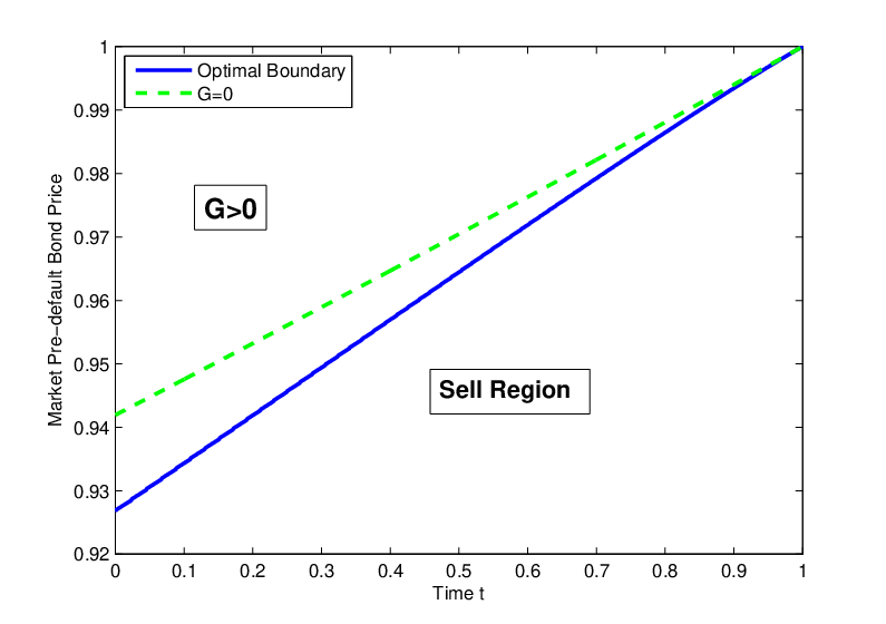
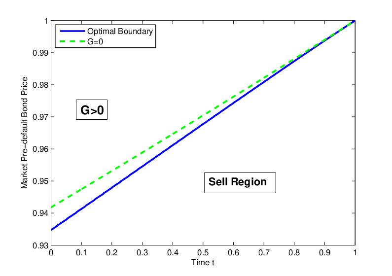
In the left panel of Figure 1, we assume that the investor agrees with the market on all parameters, but has a higher speed of mean reversion $\tilde{\kappa}_{\lambda}>\kappa_{\lambda}$ . In this case, the investor tends to sell the bond at a high market price, which is consistent with our previous analysis in terms of drift function. If the bond price starts below $0.958$ at time $0$ , the optimal liquidation strategy for the investor is to hold and sell the bond as soon as the price hits the optimal boundary. If the bond price starts above $0.958$ at time $0$ , the optimal liquidation strategy is to sell immediately. In the opposite case where $\tilde{\kappa}_{\lambda}<\kappa_{\lambda}$ (see Figure 1(right)), the optimal liquidation strategy is reversed – it is optimal to sell at a lower boundary. In each cases, the sell region must lie within where $G$ is non-positive, and the straight line defined by $G=0$ can be viewed as a linear approximation of the optimal liquidation boundary.

Under the CIR dynamics in Section 3.1, $C^{0}$ admits closed-form formula [41, §7.2]

\displaystyle C^{0}(t,{\bf x})=\prod_{i=1}^{n}{\mathbb{E}}^{\mathbb{Q}}\big\{e^{-\int_{t}^{T}\!(w^{r}_{i}+\mu w^{\lambda}_{i})X_{v}^{i}dv}|{\bf X}_{t}={\bf x}\big\}=\prod_{i=1}^{n}A_{i}(T-t)e^{-B_{i}(T-t)x_{i}},

(4.6)

where

	$\displaystyle A_{i}(s)$	$\displaystyle=[\frac{2\Xi_{i}e^{(\Xi_{i}+\kappa_{i})s/2}}{(\Xi_{i}+\kappa_{i})(e^{\Xi_{i}s}-1)+2\Xi_{i}}]^{2\kappa_{i}\theta_{i}/\sigma_{i}^{2}},$		(4.7)
	$\displaystyle B_{i}(s)$	$\displaystyle=\frac{2(e^{\Xi_{i}s}-1)(w^{r}_{i}+\mu w^{\lambda}_{i})}{(\Xi_{i}+\kappa_{i})(e^{\Xi_{i}s}-1)+2\Xi_{i}},\quad\,\text{ and }\,\quad\Xi_{i}=\sqrt{\kappa_{i}^{2}+2\sigma_{i}^{2}(w^{r}_{i}+\mu w^{\lambda}_{i})}.$		(4.8)

Refer to caption — Figure 1: Optimal liquidation boundary in terms of market pre-default bond price under OU dynamics. We take $T=1$ , $r=0.03$ , $\sigma=0.02$ , $\mu=\tilde{\mu}=2$ , and $\theta_{\lambda}=\tilde{\theta}_{\lambda}=0.015$ . *Left panel*: When $\kappa_{\lambda}=0.2<0.3=\tilde{\kappa}_{\lambda}$ , the optimal boundary increases from $0.958$ to $1$ over time. *Right panel*: When $\kappa_{\lambda}=0.3>0.2=\tilde{\kappa}_{\lambda}$ , the optimal boundary increases from $0.927$ to $1$ over time. The dashed straight line is defined by $G=0$ , and we have $G\leq 0$ in both sell regions.

As a result, the drift function is given by

\displaystyle G^{0}(t,{\bf x})=\big[\sum_{i=1}^{n}\big([B_{i}(T-t)(\tilde{\kappa}_{i}-\kappa_{i})-(\tilde{\mu}-\mu)w^{\lambda}_{i}]x_{i}+B_{i}(T-t)(\kappa_{i}\theta_{i}-\tilde{\kappa}_{i}\tilde{\theta}_{i})\big)\big]C^{0}(t,{\bf x}),

which is again linear in terms of $C^{0}(t,{\bf x})$ .

To illustrate the optimal liquidation strategy, we consider a numerical example where interest rate is constant, ${\bf X}$ = $\lambda$ , and ${\bf w}^{\lambda}=\frac{1}{\mu}$ . The benchmark specifications for the market default intensity $\lambda$ in the CIR dynamics are $T=1$ , $\mu=2$ , $\kappa_{\lambda}=0.2$ , $\theta_{\lambda}=0.015$ , $r=0.03$ , and $\sigma=0.07$ based on the estimates from [14, 15]. Like in the OU model, we can again express the sell region and delay region in terms of the pre-default market price $C^{0}$ ; see Figure 2.

4.2 Recovery of Treasury and Market Value

Extending the preceding analysis on defaultable bonds, we incorporate two principle ways of modeling recovery: the recovery of treasury or market value.

By the recovery of treasury, we assume that a recovery of $c$ times the value of the equivalent default-free bond is paid upon default. Therefore, the market pre-default bond price function is

C^{RT}(t,{\bf x})=(1-c)C^{0}(t,{\bf x})+c\beta(t,{\bf x}),

(4.9)

where $\beta(t,{\bf x}):={\mathbb{E}}^{\mathbb{Q}}\big\{e^{-\int_{t}^{T}\!r_{v}dv}|{\bf X}_{t}={\bf x}\big\}$ is the equivalent default-free bond price. Then, applying Theorem 3.4 with the quadruple $(1,0,c\beta,\tau_{d})$ , we obtain the corresponding drift function:

\displaystyle G^{RT}(t,{\bf x})=-\big(\nabla_{x}C^{RT}(t,{\bf x})\big)^{T}\Sigma(t,{\bf x}){\boldsymbol{\phi}}^{\tilde{{\mathbb{Q}}},{\mathbb{Q}}}(t,{\bf x})+(c-1)\big(\tilde{\mu}(t,{\bf x})-\mu(t,{\bf x})\big)\hat{\lambda}(t,{\bf x})C^{0}(t,{\bf x}).

(4.10)

If $c=0$ , then $C^{RT}(t,{\bf x})=C^{0}(t,{\bf x})$ and $G^{RT}$ in (4.10) reduces to the drift function of the zero-recovery bond. If $c=1$ , then $C^{RT}(t,{\bf x})=\beta(t,{\bf x})$ is the market price of a default-free bond, and risk premium discrepancy may arise only from the interest rate dynamics.

Here are two examples where the drift function $G^{RT}$ in (4.10) can be computed explicitly.

Example 4.1.

Under OU model, $C^{RT}(t,r,\lambda)$ is computed according to (4.9) with $C^{0}(t,r,\lambda)$ in (4.2) and $\beta(t,r,\lambda)=e^{\bar{A}(T-t)-B(T-t)r}$ , where $\bar{A}(s)=\int_{0}^{s}\!\big[\frac{1}{2}\sigma_{r}^{2}B^{2}(z)-\kappa_{r}\theta_{r}B(z)\big]\,dz$ and $B(s)$ is defined in (4.3).

Example 4.2.

Under the multi-factor CIR model, $C^{RT}(t,{\bf x})$ is found again from (4.9), where $C^{0}(t,{\bf x})$ is given in (4.6), and $\beta(t,{\bf x})$ is computed from (4.6) with ${\bf w}^{\lambda}={\bf 0}$ in (4.7) and (4.8).

As for the recovery of market value, we assume that at default the recovery is $c$ times the pre-default value $C^{RMV}_{\tau_{d}-}$ . The market pre-default price is given by

\displaystyle C^{RMV}(t,{\bf X}_{t})={\mathbb{E}}^{\mathbb{Q}}\big\{e^{-\int_{t}^{T}\!(r_{v}+(1-c)\lambda_{v})dv}|{\mathcal{F}}_{t}\big\},\quad 0\leq t\leq T.

(4.11)

The corresponding drift function can be obtained by applying the quadruple $(1,0,cC^{RMV},\tau_{d})$ to Theorem 3.4.

Example 4.3.

Under the OU model in Section 3.1, the price function $C^{RMV}(t,r,\lambda)$ is given by

C^{RMV}(t,r,\lambda)=e^{\hat{A}(T-t)-B(T-t)r-\hat{D}(T-t)\lambda},

where $B(s)$ is defined in (4.3),

	$\displaystyle\hat{D}(s)$	$\displaystyle=\frac{(1-c)(1-e^{-\kappa_{\lambda}s})}{\kappa_{\lambda}},~\text{ and}$
	$\displaystyle\hat{A}(s)$	$\displaystyle=\int_{0}^{s}\!\big[\frac{1}{2}\sigma_{r}^{2}B^{2}(z)+\rho\mu\sigma_{r}\sigma_{\lambda}B(z)\hat{D}(z)+\frac{1}{2}\mu^{2}\sigma_{\lambda}^{2}\hat{D}^{2}(z)-\kappa_{r}\theta_{r}B(z)-\mu\kappa_{\lambda}\theta_{\lambda}\hat{D}(z)\big]dz.$

Example 4.4.

Under the multi-factor CIR model, $C^{RMV}(t,{\bf x})$ admits the same formula as (4.6) but with ${\boldsymbol{w}^{\lambda}}$ replaced by $(1-c){\boldsymbol{w}^{\lambda}}$ in (4.7) and (4.8).

4.3 Optimal Liquidation of CDS

In this section we consider optimally liquidating a digital CDS position. The investor is a protection buyer who pays a fixed premium to the protection seller from time $0$ until default or maturity $T$ , whichever comes first. The premium rate $p^{m}_{0}$ , called the market spread, is specified at contract inception. In return, the protection buyer will receive $ $1$ if default occurs at or before $T$ . The liquidation of the CDS position at time $t$ can be achieved by entering a CDS contract as a protection seller with the same credit reference and same maturity $T$ at the prevailing market spread $p^{m}_{t}$ . By definition, the prevailing market spread $p^{m}_{t}$ makes the values of two legs equal at time $t$ , i.e.

\displaystyle{\mathbb{E}}^{\mathbb{Q}}\big\{\int_{t}^{T}\!e^{-\int_{t}^{u}\!r_{v}dv}p^{m}_{t}{\mathbf{1}}_{\{u<\tau_{d}\}}du|{\mathcal{G}}_{t}\big\}={\mathbb{E}}^{\mathbb{Q}}\big\{e^{-\int_{t}^{\tau_{d}}\!r_{v}dv}{\mathbf{1}}_{\{t<\tau_{d}\leq T\}}|{\mathcal{G}}_{t}\big\}.

(4.12)

If the liquidation occurs at time $t$ , she receives the premium at rate $p^{m}_{t}$ and pays the premium at rate $p^{m}_{0}$ until default or maturity $T$ . If default occurs, then the default payments from both CDS contracts will cancel. Considering the resulting expected cash flows and (4.12), the mark-to-market value of the CDS is given by

	$\displaystyle{\mathbb{E}}^{\mathbb{Q}}\big\{\int_{t}^{T}\!e^{-\int_{t}^{u}\!r_{v}dv}(p^{m}_{t}-p^{m}_{0}){\mathbf{1}}_{\{u<\tau_{d}\}}du\|{\mathcal{G}}_{t}\big\}=$	$\displaystyle{\mathbf{1}}_{\{t<\tau_{d}\}}{\mathbb{E}}^{\mathbb{Q}}\big\{\int_{t}^{T}\!e^{-\int_{t}^{u}\!(r_{v}+\lambda_{v})dv}(\lambda_{u}-p^{m}_{0})du\|{\mathcal{F}}_{t}\big\}$
	$\displaystyle=$	$\displaystyle:{\mathbf{1}}_{\{t<\tau_{d}\}}C^{CDS}(t,{\bf X}_{t}).$		(4.13)

For CDS, we apply the quadruple $(0,-p^{m}_{0},1,\tau_{d})$ to Theorem 3.4 and obtain the drift function:

\displaystyle G^{CDS}(t,{\bf x})=-\big(\nabla_{x}C^{CDS}(t,{\bf x})\big)^{T}\Sigma(t,{\bf x}){\boldsymbol{\phi}}^{\tilde{{\mathbb{Q}}},{\mathbb{Q}}}(t,{\bf x})+\big(1-C^{CDS}(t,{\bf x})\big)\big(\tilde{\mu}(t,{\bf x})-\mu(t,{\bf x})\big)\hat{\lambda}(t,{\bf x}).

(4.14)

If there is no discrepancy over mark-to-market risk premium, i.e. ${\boldsymbol{\phi}}^{\tilde{{\mathbb{Q}}},{\mathbb{Q}}}(t,{\bf x})={\bf 0}$ , then the sign of $G^{CDS}$ is determined by $\tilde{\mu}(t,{\bf x})-\mu(t,{\bf x})$ since $C^{CDS}\leq 1$ . From this we infer that higher event risk premium (relative to market) implies delayed liquidation.

In general, the market pre-default value $C^{CDS}$ can be solved by PDE (3.1). If the state vector ${\bf X}$ admits OU or CIR dynamics, $C^{CDS}$ , and thus $G^{CDS}$ , is given in closed form, as illustrated in the following two examples.

Example 4.5.

Under the OU dynamics, the pre-default value of CDS (see (4.13)) is given by the following integral:

\displaystyle C^{CDS}(t,r,\lambda)=\int_{t}^{T}\!C^{0}(t,r,\lambda;u)\bigg[\lambda e^{-\kappa_{\lambda}(u-t)}+\int_{t}^{u}\!e^{-\kappa_{r}(u-s)}g(s,u)ds-p^{m}_{0}\bigg]du,

where $C^{0}(t,r,\lambda;u)$ is given by (4.2) with $T=u$ and

\displaystyle g(s,u):=\mu\kappa_{\lambda}\theta_{\lambda}-\rho\mu\sigma_{r}\sigma_{\lambda}\frac{1-e^{-\kappa_{r}(u-s)}}{\kappa_{r}}-(\mu\sigma_{\lambda})^{2}\frac{1-e^{-\kappa_{\lambda}(u-s)}}{\kappa_{\lambda}}.

Example 4.6.

Under the multi-factor CIR dynamics, the pre-default value of CDS is given by the following integral:

\displaystyle C^{CDS}(t,{\bf x})=\int_{t}^{T}\!C^{0}(t,{\bf x};u)\bigg[\displaystyle\sum_{i=1}^{n}\bigg(\mu w^{\lambda}_{i}\big(\kappa_{i}\theta_{i}B_{i}(u-t)+B_{i}^{\prime}(u-t)x_{i}\big)\bigg)-p^{m}_{0}\bigg]du,

where $C^{0}(t,{\bf x};u)$ is given in (4.6) with $T=u$ and $B_{i}(s)$ in (4.8). See Chapter $7$ of [41].

Example 4.7.

For a forward CDS with start date $T_{a}<T$ , the protection buyer pays premium at rate $p_{a}$ from $T_{a}$ until $\tau_{d}$ or maturity $T$ , and receives $1$ if $\tau_{d}\in[T_{a},T]$ . By direct computation, the pre-default market value is $C^{CDS}(t,{\bf x};T)-C^{CDS}(t,{\bf x};T_{a})$ , $t<T_{a}$ . Consequently, closed-form formulas for the drift function are available under OU or CIR dynamics by Examples 4.5 and 4.6.

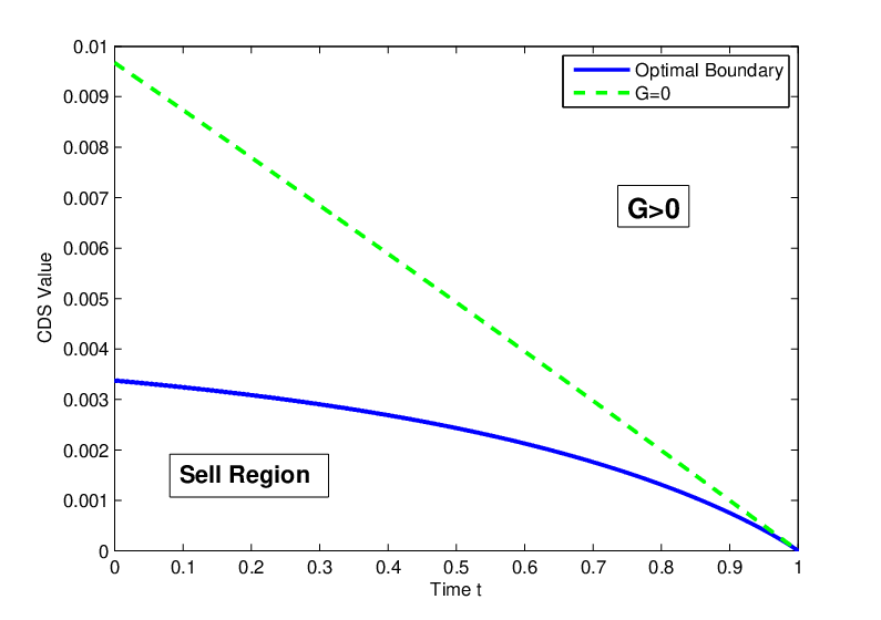
We consider a numerical example where interest rate is constant and state vector ${\bf X}$ = $\lambda$ follows the CIR dynamics. We assume that the investor agrees with the market on all parameters except the speed of mean reversion for default intensity. In the left panel of Figure 3 with $\kappa_{\lambda}=0.2<0.3=\tilde{\kappa}_{\lambda}$ , the optimal liquidation strategy is to sell as soon as the market CDS value reaches an upper boundary. In the case with $\kappa_{\lambda}=0.3>0.2=\tilde{\kappa}_{\lambda}$ (see Figure 3 (right)), the sell region is below the continuation region.

Remark 4.8.

As a straightforward generalization under our framework, one can replace the unit payment at default by $R^{CDS}(\tau_{d},{\bf X_{\tau_{d}}})$ . Then, we can apply the quadruple $(0,-p^{m}_{0},R^{CDS},\tau_{d})$ to Theorem 3.4, and obtain the same drift function $G^{CDS}$ in (4.14) except with $1$ replaced by $R^{CDS}(t,{\bf x})$ .

4.4 Jump-Diffusion Default Intensity

We can extend our analysis to incorporate jumps to the stochastic state vector. To illustrate this, suppose the default intensity and interest rate are driven by a $n$ -dimensional state vector ${\bf X}^{\prime}$ with the affine jump-diffusion dynamics:

\displaystyle d{\bf X}^{\prime}_{t}=a(t,{\bf X}^{\prime}_{t})dt+\Sigma(t,{\bf X}^{\prime}_{t})d{\bf W}^{\mathbb{P}}_{t}+d{\bf J}_{t},

(4.15)

where ${\bf J}=(J^{1},\ldots,J^{n})^{T}$ is a vector of $n$ independent pure jump processes taking values in ${\mathbb{R}}^{n}$ . Under historical measure ${\mathbb{P}}$ , we assume Markovian jump intensity of the form $\hat{\bf{\Lambda}}(t,{\bf X}^{\prime}_{t})=(\hat{\Lambda}^{1}(t,{\bf X}^{\prime}_{t}),\ldots,\hat{\Lambda}^{n}(t,{\bf X}^{\prime}_{t}))^{T}$ for ${\bf J}$ . All random jump sizes $(Y^{i}_{j})_{ij}$ of ${\bf J}$ are independent, and for each $J^{i}$ , the associated jump sizes $Y^{i}_{1},Y^{i}_{2},\ldots$ have a common probability density function $\hat{f}^{i}$ .

The default intensity of defaultable security is given by $\hat{\lambda}(t,{\bf X}^{\prime}_{t})$ for some positive measurable function $\hat{\lambda}(\cdot,\cdot)$ , and the default counting process associated with default time $\tau_{d}$ is denoted by $N_{t}={\mathbf{1}}_{\{t\geq\tau_{d}\}}$ . We denote $(\mathcal{G}_{t})_{0\leq t\leq T}$ to be the full filtration generated by ${\bf W}^{\mathbb{P}},{\bf J}$ , and $\tau_{d}$ .

We define a market pricing measure ${\mathbb{Q}}$ in terms of the mark-to-market risk premium ${\boldsymbol{\phi}}^{{\mathbb{Q}},{\mathbb{P}}}$ and event risk premium $\mu$ , which are Markovian and satisfy $\int_{0}^{T}|\!|{\boldsymbol{\phi}}^{{{\mathbb{Q}}},{\mathbb{P}}}_{u}|\!|^{2}du<\infty$ and $\int_{0}^{T}\mu_{u}\hat{\lambda}_{u}du<\infty$ . Due to the presence of ${\bf J}$ , the market measure ${\mathbb{Q}}$ can scale the jump intensity of ${\bf J}$ by the positive Markovian factors $\delta_{t}^{i}=\delta^{i}(t,{\bf X}^{\prime}_{t})$ , with $\int_{0}^{T}\delta^{i}_{u}\hat{\Lambda}^{i}_{u}du<\infty$ for $i=1,\ldots,n$ . Also, ${\mathbb{Q}}$ can transform the jump size distribution of ${\bf J}$ by a function $(h^{i})_{i=1,\ldots,n}>0$ satisfying $\int_{0}^{\infty}h^{i}(y)\hat{f}^{i}(y)dy=1$ for $i=1,\ldots,n$ .

The Radon-Nikodym derivative is given by

\displaystyle\frac{d{{\mathbb{Q}}}}{d{\mathbb{P}}}\big|\mathcal{G}_{t}=\mathcal{E}\big(-{\boldsymbol{\phi}}^{{\mathbb{Q}},{\mathbb{P}}}\!\cdot\!{\bf W}^{\mathbb{P}}\big)_{t}\,\mathcal{E}\big((\mu-1)M^{\mathbb{P}}\big)_{t}K_{t}^{{\mathbb{Q}},{\mathbb{P}}},

where first two Doléans-Dade exponentials are defined in (3.3) and (3.4) respectively, $M^{\mathbb{P}}_{t}:=N_{t}-\int_{0}^{t}\!(1-N_{u})\hat{\lambda}_{u}du$ is the compensated ${\mathbb{P}}$ -martingale associated with $N$ , and the last term

\displaystyle K_{t}^{{\mathbb{Q}},{\mathbb{P}}}:=\prod_{i=1}^{n}\bigg[\exp\bigg(\int_{0}^{t}\int_{{\mathbb{R}}^{n}}{\big(1-\delta^{i}(u,{\bf X}^{\prime}_{u})h^{i}(y)\big)\hat{\Lambda}^{i}(u,{\bf X}^{\prime}_{u})\hat{f}^{i}(y)d{y}du}\bigg)\prod_{j=1}^{N^{(i)}_{t}}\,\big(\delta^{i}(T_{j}^{i},{\bf X}^{\prime}_{T_{j}^{i}})h^{i}(Y^{i}_{j})\big)\bigg],

where $T^{i}_{j}$ is the $j$ th jump time of $J^{i}$ and $N_{t}^{(i)}:=\sum_{j\geq 1}{\mathbf{1}}_{\{T^{i}_{j}\leq t\}}$ is the counting process associated with $J^{i}$ .

By Girsanov Theorem, ${\bf W}^{{\mathbb{Q}}}_{t}:={\bf W}^{\mathbb{P}}_{t}+\int_{0}^{t}{\boldsymbol{\phi}}_{u}^{{\mathbb{Q}},{\mathbb{P}}}du$ is a ${\mathbb{Q}}$ -Brownian motion, the jump intensity of $J^{i}$ under ${\mathbb{Q}}$ is $\Lambda^{i}(t,{\bf X}^{\prime}_{t}):=\delta^{i}(t,{\bf X}^{\prime}_{t})\hat{\Lambda}^{i}(t,{\bf X}^{\prime}_{t})$ , and the jump size pdf of $J^{i}$ under ${\mathbb{Q}}$ is $f^{i}(y):=h^{i}(y)\hat{f}^{i}(y)$ . The ${\mathbb{Q}}$ -dynamics of state vector ${\bf X}^{\prime}$ is given by

\displaystyle d{\bf X}^{\prime}_{t}=b(t,{\bf X}^{\prime}_{t})dt+\Sigma(t,{\bf X}^{\prime}_{t})d{\bf W}^{\mathbb{Q}}_{t}+d{\bf J}_{t}.

(4.16)

Also incorporating the event risk premium, the ${\mathbb{Q}}$ -default intensity is $\lambda(t,{\bf X}^{\prime}_{t}):=\mu(t,{\bf X}^{\prime}_{t})\hat{\lambda}(t,{\bf X}^{\prime}_{t})$ .

Under the investor’s measure $\tilde{{\mathbb{Q}}}$ , we replace $b$ with $\tilde{b}$ , ${\boldsymbol{\phi}}^{{\mathbb{Q}},{\mathbb{P}}}$ with ${\boldsymbol{\phi}}^{\tilde{{\mathbb{Q}}},{\mathbb{P}}}$ , and ${\bf W}^{\mathbb{Q}}$ with ${\bf W}^{\tilde{{\mathbb{Q}}}}$ for the dynamics of ${\bf X}^{\prime}$ . For each $J^{i}$ , the $\tilde{{\mathbb{Q}}}$ -intensity is denoted by $\tilde{\Lambda}^{i}(t,{\bf X}^{\prime}_{t}):={\tilde{\delta}}^{i}(t,{\bf X}^{\prime}_{t})\hat{\Lambda}^{i}(t,{\bf X}^{\prime}_{t})$ , and the jump size pdf under $\tilde{{\mathbb{Q}}}$ is $\tilde{f}^{i}(y):=\tilde{h}^{i}(y)\hat{f}^{i}(y)$ . With investor’s event risk premium $\tilde{\mu}$ , the default intensity under $\tilde{{\mathbb{Q}}}$ is $\tilde{\lambda}(t,{\bf X}^{\prime}_{t}):=\tilde{\mu}(t,{\bf X}^{\prime}_{t})\hat{\lambda}(t,{\bf X}^{\prime}_{t})$ .

The two pricing measures ${\mathbb{Q}}$ and $\tilde{{\mathbb{Q}}}$ are related by the Radon-Nikodym derivative:

\displaystyle\frac{d\tilde{{\mathbb{Q}}}}{d{\mathbb{Q}}}\big|\mathcal{G}_{t}=\mathcal{E}\big(-{\boldsymbol{\phi}}^{\tilde{{\mathbb{Q}}},{\mathbb{Q}}}\!\cdot\!{\bf W}^{\mathbb{Q}}\big)_{t}\,\mathcal{E}\big((\frac{\tilde{\mu}}{\mu}-1)M^{\mathbb{Q}}\big)_{t}K_{t}^{\tilde{{\mathbb{Q}}},{\mathbb{Q}}},

where $M^{\mathbb{Q}}_{t}:=N_{t}-\int_{0}^{t}\!(1-N_{u})\lambda_{u}du$ is the compensated ${\mathbb{Q}}$ -martingale associated with $N$ , the first two Doléans-Dade exponentials are defined in (3.7) and (3.8), and

\displaystyle K_{t}^{\tilde{{\mathbb{Q}}},{\mathbb{Q}}}:=\prod_{i=1}^{n}\bigg[\exp\bigg(\int_{0}^{t}\int_{{\mathbb{R}}^{n}}{\big(\Lambda^{i}(u,{\bf X}^{\prime}_{u})f^{i}(y)-\tilde{\Lambda}^{i}(u,{\bf X}^{\prime}_{u})\tilde{f}^{i}(y)\big)dydu}\bigg)\prod_{j=1}^{N^{(i)}_{t}}\,\frac{\tilde{\Lambda}^{i}(T^{i}_{j},{\bf X}^{\prime}_{T^{i}_{j}})\tilde{f}^{i}({\bf Y}^{i}_{j})}{\Lambda^{i}(T^{i}_{j},{\bf X}^{\prime}_{T^{i}_{j}})f^{i}({\bf Y}^{i}_{j})}\bigg].

Consequently, on top of the mark-to-market risk and event risk premia, the investor can potentially disagree with the market over jump intensity and jump size distribution of ${\bf X}^{\prime}$ , allowing for a richer structure of price discrepancy as well as the optimal liquidation strategy.

As in Theorem 3.4, we compute the drift function in terms of pre-default price $C$ and default risk premia, namely,

	$\displaystyle G^{J}(t,{\bf x})$	$\displaystyle=-\big(\nabla_{x}C(t,{\bf x})\big)^{T}\Sigma(t,{\bf x}){\boldsymbol{\phi}}^{\tilde{{\mathbb{Q}}},{\mathbb{Q}}}(t,{\bf x})+(R(t,{\bf x})-C(t,{\bf x}))\big(\tilde{\mu}(t,{\bf x})-\mu(t,{\bf x})\big)\hat{\lambda}(t,{\bf x})$
		$\displaystyle+\sum_{i=1}^{n}\bigg(\int_{{\mathbb{R}}^{n}}{\big(C(t,{\bf x}+y{\bf e}_{i})-C(t,{\bf x})\big)\big(\tilde{\Lambda}^{i}(t,{\bf x})\tilde{f}^{i}(y)-\Lambda^{i}(t,{\bf x})f^{i}(y)\big)dy}\bigg),$		(4.17)

where ${\bf e}_{i}:=(0,\ldots,1,\ldots,0)^{T}$ . We observe that the first two components of $G^{J}$ share the same functional form as $G$ in (3.20), though the price function $C$ is derived from the jump-diffusion model. Even if the investor and the market assign the same mark-to-market risk and event risk premia, discrepancy over jump intensity and distribution will yield different liquidation strategies. Under quite general affine jump-diffusion models, Duffie et al. [17] provide an analytical treatment of transform analysis, which can be used for the computation of our drift function.

5 Optimal Liquidation of Credit Default Index Swaps

We proceed to discuss the optimal liquidation of multi-name credit derivatives. In the literature, there exist many proposed models for modeling multiple defaults and pricing multi-name credit derivatives. Within the intensity-based framework, one popular approach is to model each default time by the first jump of a doubly-stochastic process. The dependence among defaults can be incorporated via some common stochastic factors. This well-known bottom-up valuation framework has been studied in [16, 38], among many others.

As a popular alternative, the top-down approach describes directly the dynamics of the cumulative credit portfolio loss, without detailed references to the constituent single names. Some examples of top-down models include [3, 8, 13, 36, 37]. In particular, Errais et al. [20] proposed affine point processes for portfolio loss with self-exciting property to capture default clustering. For our analysis, rather than proposing a new multi-name credit risk model, we adopt the self-exciting top-down model from [20]. Also, we will focus on the optimal liquidation of a credit default index swap.

First, we model successive default arrivals by a counting process $(N_{t})_{0\leq t\leq T}$ , and the accumulated portfolio loss by $\Upsilon_{t}=l_{1}+\ldots+l_{N_{t}}$ , with each $l_{n}$ representing the random loss at the $n$ th default. Under the historical measure ${\mathbb{P}}$ , the default intensity evolves according to the jump-diffusion:

\displaystyle d\hat{\lambda}_{t}=\hat{\kappa}(\hat{\theta}-\hat{\lambda}_{t})dt+\sigma\sqrt{\hat{\lambda}_{t}}\,dW_{t}^{\mathbb{P}}+\eta\,d\Upsilon_{t},

(5.1)

where $W^{\mathbb{P}}$ is a standard ${\mathbb{P}}$ -Brownian motion. We assume that the random losses $(l_{n})$ are independent with an identical probability density function $\hat{m}$ on $(0,\infty)$ . According to the last term in (5.1), each default arrival will increase default intensity $\hat{\lambda}$ by the loss at default scaled by the positive parameter $\eta$ . This term captures default clustering observed in the multi-name credit derivatives as pointed out in [20]. We assume a constant risk-free interest rate $r$ for simplicity, and denote $(\mathcal{H}_{t})_{0\leq t\leq T}$ to be the full filtration generated by $N$ , $\Upsilon$ , and $W^{\mathbb{P}}$ .

The market measure ${\mathbb{Q}}$ is characterized by several key components. First, the market’s mark-to-market risk premium is assumed to be of the form

\displaystyle{\phi}_{t}^{{\mathbb{Q}},{\mathbb{P}}}=\frac{\hat{\kappa}(\hat{\theta}-\hat{\lambda}_{t})-\kappa(\theta-\hat{\lambda}_{t})}{\sigma\sqrt{\hat{\lambda}_{t}}}

(5.2)

such that the default intensity in (5.1) preserves mean-reverting dynamics with different parameters $\kappa$ and $\theta$ under the market measure ${\mathbb{Q}}$ (see [4, 27] for similar specifications). Secondly, we assume that the ${\mathbb{Q}}$ -default intensity is $\lambda_{t}:=\mu\hat{\lambda}_{t}$ , with a positive constant event risk premium. Thirdly, the distribution of random losses can be scaled under ${\mathbb{Q}}$ . Specifically, we assume that under ${\mathbb{Q}}$ the losses $(l_{n})$ admit the pdf $m(z):=h(z)\hat{m}(z)$ , for some strictly positive function $h$ with $\int_{0}^{\infty}h(z)\hat{m}(z)dz=1$ . Then, the Radon-Nikodym derivative associated with ${\mathbb{Q}}$ and ${\mathbb{P}}$ is

\displaystyle\frac{d{\mathbb{Q}}}{d{\mathbb{P}}}\big|\mathcal{H}_{t}=\mathcal{E}\big(-{\phi}^{{\mathbb{Q}},{\mathbb{P}}}W^{\mathbb{P}}\big)_{t}\hat{K}^{{\mathbb{Q}},{\mathbb{P}}}_{t}\,,

(5.3)

where $\mathcal{E}\big(-{\phi}^{{\mathbb{Q}},{\mathbb{P}}}W^{\mathbb{P}}\big)$ is defined in (3.3), and

\displaystyle\hat{K}_{t}^{{\mathbb{Q}},{\mathbb{P}}}:=\exp\bigg(\int_{0}^{t}\int_{0}^{\infty}{\big(1-\mu h(z)\big)\hat{\lambda}_{u}\hat{m}(z)dzdu}\bigg)\prod_{i=1}^{N_{t}}\,\big(\mu h(l_{i})\big).

(5.4)

Under the market pricing measure ${\mathbb{Q}}$ , the ${\mathbb{Q}}$ -default intensity evolves according to:

\displaystyle d{\lambda}_{t}=\kappa(\mu\theta-{\lambda}_{t})dt+\sigma\sqrt{\mu{\lambda}_{t}}\,dW_{t}^{\mathbb{Q}}+\mu\eta\,d\Upsilon_{t},

(5.5)

where ${W}^{{\mathbb{Q}}}_{t}:={W}^{\mathbb{P}}_{t}+\int_{0}^{t}{\phi}_{u}^{{\mathbb{Q}},{\mathbb{P}}}du$ is a standard ${\mathbb{Q}}$ -Brownian motion. Similarly, we can define the investor’s pricing measure $\tilde{{\mathbb{Q}}}$ through the investor’s mark-to-market risk premium ${\phi}^{\tilde{{\mathbb{Q}}},{\mathbb{P}}}$ as in (5.2) with parameters $\tilde{\kappa}$ and $\tilde{\theta}$ ; default intensity $\tilde{\lambda}_{t}=\tilde{\mu}\hat{\lambda}_{t}$ with constant event risk premium $\tilde{\mu}$ ; and loss scaling function $\tilde{h}$ so that the loss pdf $\tilde{m}(z)=h(z)\hat{m}(z)$ .

The credit default index swap is written on a standardized portfolio of $H$ reference entities, such as single-name default swaps, with same notational normalized to $1$ and same maturity $T$ . The investor is a protection buyer who pays at the premium rate $p^{m}_{0}$ in return for default payments over $(0,T]$ . Here, the default payment is assumed to be paid at the time when default occurs, and the premium payment is paid continuously with premium notational equal to $H-N_{t}$ .

The market’s cumulative value of the credit default index swap for the protection buyer is equal to the difference between the market values of the default payment leg and premium leg, namely,

\displaystyle P^{CDX}_{t}={\mathbb{E}}^{\mathbb{Q}}\big\{\int_{(0,T]}e^{-r(u-t)}\ d\Upsilon_{u}\,|\mathcal{H}_{t}\big\}-{\mathbb{E}}^{\mathbb{Q}}\big\{p^{m}_{0}\int_{(0,T]}e^{-r(u-t)}(H-N_{u})\,du\,|\mathcal{H}_{t}\big\},\quad t\leq T.

(5.6)

Hence, similar to (2.7), the protection buyer solves the following optimal stopping problem:

\displaystyle V^{CDX}_{t}=\esssup_{\tau\in\mathcal{T}_{t,T}}~{\mathbb{E}}^{\tilde{{\mathbb{Q}}}}\big\{e^{-r(\tau-t)}P^{CDX}_{\tau}\,|\mathcal{H}_{t}\big\}.

(5.7)

The associated delayed liquidation premium is defined by

\displaystyle L^{CDX}_{t}=V^{CDX}_{t}-P^{CDX}_{t}.

(5.8)

The derivation of the optimal liquidation strategy involves computing the market’s ex-dividend value, defined by

\displaystyle{C}^{CDX}_{t}=

\displaystyle{\mathbb{E}}^{\mathbb{Q}}\big\{\int_{(t,T]}e^{-r(u-t)}\ d\Upsilon_{u}\,|\mathcal{H}_{t}\big\}-{\mathbb{E}}^{\mathbb{Q}}\big\{p^{m}_{0}\int_{(t,T]}e^{-r(u-t)}(H-N_{u})\,du\,|\mathcal{H}_{t}\big\}.

(5.9)

Proposition 5.1.

The market’s ex-dividend value of the credit default index swap in (5.9) can be expressed as ${C}^{CDX}_{t}={C}^{CDX}(t,\lambda_{t},N_{t})$ , where

\displaystyle{C}^{CDX}(t,\lambda,n)=k_{2}(t,T)\lambda+k_{1}(t,T)n+k_{0}(t,T),

(5.10)

for $t\leq T$ , with coefficients

		$\displaystyle k_{2}(t,T)=(cr+p^{m}_{0})\bigg(\frac{e^{-(\rho+r)(T-t)}}{\rho(\rho+r)}-\frac{e^{-r(T-t)}}{\rho r}+\frac{1}{r(\rho+r)}\bigg)+\frac{ce^{-r(T-t)}}{\rho}\big(1-e^{-\rho(T-t)}\big),$		(5.11)
		$\displaystyle k_{1}(t,T)=\frac{p^{m}_{0}\big(1-e^{-r(T-t)}\big)}{r},$		(5.12)
		$\displaystyle k_{0}(t,T)=\frac{\kappa\mu\theta}{\rho}\bigg((rc+p^{m}_{0})\big[e^{-r(T-t)}\big(-\frac{e^{-\rho(T-t)}}{\rho(\rho+r)}-\frac{T-t}{r}-\frac{1}{r^{2}}+\frac{1}{r\rho}\big)+\frac{\rho}{r^{2}(r+\rho)}\big]$
		$\displaystyle~~~~~~~~~\,+ce^{-r(T-t)}\big(\frac{e^{-\rho(T-t)}-1}{\rho}+T-t\big)\bigg)-\frac{p^{m}_{0}H}{r}\big(1-e^{-r(T-t)}\big),$		(5.13)

and constants

\displaystyle c=\int_{0}^{\infty}zm(z)dz,\qquad\text{and }\qquad\rho=\kappa-\mu\eta c.

(5.14)

Proof.

Using integration by parts, we re-write the market’s ex-dividend value as

\displaystyle{C}^{CDX}_{t}=e^{-r(T-t)}\ {\mathbb{E}}^{\mathbb{Q}}\{\Upsilon_{T}|\mathcal{H}_{t}\}-\Upsilon_{t}+\int_{t}^{T}{e^{-r(u-t)}\ \big[r{\mathbb{E}}^{\mathbb{Q}}\{\Upsilon_{u}|\mathcal{H}_{t}\}-p^{m}_{0}\big(H-{\mathbb{E}}^{\mathbb{Q}}\{N_{u}|\mathcal{H}_{t}\}\big)\big]\,du}.

(5.15)

Hence, the computation of ${C}^{CDX}$ involves calculating ${\mathbb{E}}^{\mathbb{Q}}\{N_{u}\,|\,\mathcal{H}_{t}\}$ and ${\mathbb{E}}^{\mathbb{Q}}\{\Upsilon_{u}\,|\,\mathcal{H}_{t}\}$ , $u\geq t$ . Since default intensity $\lambda$ follows a square-root jump-diffusion dynamics, these conditional expectation admit the closed-form formulas (see e.g. Section $4.3$ of [20]):

	$\displaystyle{\mathbb{E}}^{\mathbb{Q}}\{N_{u}\,\|\,\lambda_{t}$	$\displaystyle=\lambda,N_{t}=n,\Upsilon_{t}=\upsilon\}=\mathcal{A}(t,u)+\mathcal{B}(t,u)\lambda+n,$		(5.16)
	$\displaystyle{\mathbb{E}}^{\mathbb{Q}}\{\Upsilon_{u}\,\|\,\lambda_{t}$	$\displaystyle=\lambda,N_{t}=n,\Upsilon_{t}=\upsilon\}=c\mathcal{A}(t,u)+c\mathcal{B}(t,u)\lambda+\upsilon,$		(5.17)

for $t\leq u\leq T$ , where

	$\displaystyle\mathcal{A}(t,u)$	$\displaystyle=\frac{\kappa\mu\theta}{\kappa-\mu\eta c}\big(\frac{e^{-(\kappa-\mu\eta c)(u-t)}-1}{\kappa-\mu\eta c}+u-t\big),$		(5.18)
	$\displaystyle\mathcal{B}(t,u)$	$\displaystyle=\frac{1}{\kappa-\mu\eta c}(1-e^{-(\kappa-\mu\eta c)(u-t)}).$		(5.19)

Here, $c$ is the market’s expected loss at default given in (5.14). Substituting (5.16) and (5.17) into (5.15), we obtain the closed-form formula for market’s ex-dividend value in (5.10). ∎

As a result, the ex-dividend value ${C}^{CDX}$ is linear in the default intensity $\lambda_{t}$ and number of defaults $N_{t}$ . Next, we characterize the optimal corresponding liquidation premium and strategy.

Theorem 5.2.

Under the top-down credit risk model in (5.1), the delayed liquidation premium associated with the credit default index swap is given by

\displaystyle L^{CDX}(t,\lambda)=\sup_{\tau\in\mathcal{T}_{t,T}}~{\mathbb{E}}^{\tilde{{\mathbb{Q}}}}\big\{\int_{t}^{\tau}e^{-r(u-t)}G^{CDX}(u,\lambda_{u})du\,|\,\lambda_{t}=\lambda\big\},

(5.20)

where

	$\displaystyle G^{CDX}(t,\lambda)$	$\displaystyle=\bigg(\big(\mu\eta k_{2}(t,T)+1\big)(\frac{\tilde{\mu}\tilde{c}}{\mu}-c)+k_{1}(t,T)(\frac{\tilde{\mu}}{\mu}-1)-k_{2}(t,T)(\tilde{\kappa}-\kappa)\bigg)\lambda$
		$\displaystyle~~+k_{2}(t,T)\mu(\tilde{\kappa}\tilde{\theta}-\kappa\theta),$		(5.21)

with $\tilde{c}:=\int_{0}^{\infty}z\tilde{m}(z)dz$ . If $G^{CDX}(t,\lambda)\geq 0$ $\forall(t,\lambda)$ , then it is optimal to delay the liquidation till maturity $T$ . If $G^{CDX}(t,\lambda)\leq 0$ $\forall(t,\lambda)$ , then it is optimal to sell immediately.

Proof.

In view of the definition of $L^{CDX}$ in (5.8), we consider the dynamics of $P^{CDX}$ . First, it follows from (5.6) and (5.9) that

\displaystyle e^{-r(u-t)}P^{CDX}_{u}=e^{-r(u-t)}{C}^{CDX}_{u}+\int_{(0,u]}e^{-r(v-t)}\ \big(d\Upsilon_{v}-p^{m}_{0}(H-N_{v})dv\big).

(5.22)

Using (5.22) and the fact that $e^{-rt}P^{CDX}_{t}$ is ${\mathbb{Q}}$ -martingale (whose SDE must have no drift), we apply Ito’s lemma to get

	$\displaystyle e^{-r(\tau-t)}P^{CDX}_{\tau}-P^{CDX}_{t}$
$\displaystyle=$	$\displaystyle\int_{t}^{\tau}e^{-r(u-t)}{\frac{\partial{C}^{CDX}}{\partial\lambda}}(u,\lambda_{u},N_{u})\sigma\sqrt{\mu\lambda_{u}}dW^{\mathbb{Q}}_{u}$
	$\displaystyle+\bigg[\sum_{t<u\leq\tau}e^{-r(u-t)}(\Upsilon_{u}-\Upsilon_{u_{-}})-\int_{t}^{\tau}\int_{0}^{\infty}{e^{-r(u-t)}zm(z)\lambda_{u}\,dzdu}\bigg]$
	$\displaystyle+\bigg[\sum_{t<u\leq\tau}e^{-r(u-t)}\big({C}^{CDX}(u,\lambda_{u},N_{u})-{C}^{CDX}(u,\lambda_{u-},N_{u-})\big)$
	$\displaystyle-\int_{t}^{\tau}\int_{0}^{\infty}{e^{-r(u-t)}\big({C}^{CDX}(u,\lambda_{u}+\mu\eta z,N_{u}+1)-{C}^{CDX}(u,\lambda_{u},N_{u})\big)m(z)\lambda_{u}\,dzdu}\bigg]$	(5.23)
$\displaystyle=$	$\displaystyle\int_{t}^{\tau}e^{-r(u-t)}\big({\frac{\partial{C}^{CDX}}{\partial\lambda}}(u,\lambda_{u},N_{u})\sigma\sqrt{\mu\lambda_{u}}dW^{\tilde{{\mathbb{Q}}}}_{u}+G^{CDX}(u,\lambda_{u},N_{u})du\big)$
	$\displaystyle+\bigg[\sum_{t<u\leq\tau}e^{-r(u-t)}(\Upsilon_{u}-\Upsilon_{u_{-}})-\int_{t}^{\tau}\int_{0}^{\infty}{e^{-r(u-t)}z\tilde{m}(z)\tilde{\lambda}_{u}\,dzdu}\bigg]$
	$\displaystyle+\bigg[\sum_{t<u\leq\tau}e^{-r(u-t)}\big({C}^{CDX}(u,\lambda_{u},N_{u})-{C}^{CDX}(u,\lambda_{u-},N_{u-})\big)$
	$\displaystyle-\int_{t}^{\tau}\int_{0}^{\infty}{e^{-r(u-t)}\big({C}^{CDX}(u,\lambda_{u}+\mu\eta z,N_{u}+1)-{C}^{CDX}(u,\lambda_{u},N_{u})\big)\tilde{m}(z)\tilde{\lambda}_{u}\,dzdu}\bigg],$	(5.24)

for $t\leq\tau\leq T$ , where

	$\displaystyle G^{CDX}(t,\lambda,n)$	$\displaystyle:=\frac{\partial{C}^{CDX}}{\partial\lambda}(t,\lambda,n)\big((\tilde{\kappa}\tilde{\theta}-\kappa\theta)\mu-(\tilde{\kappa}-\kappa)\lambda\big)$		(5.25)
		$\displaystyle+\int_{0}^{\infty}{\big(z+{C}^{CDX}(t,\lambda+\mu\eta z,n+1)-{C}^{CDX}(t,\lambda,n)\big)(\frac{\tilde{\mu}}{\mu}\tilde{m}(z)-m(z)\big)\lambda dz\,}.$

Note that the two compensated ${\mathbb{Q}}$ -martingale terms in (5.23) account for, respectively, losses and changes in $C^{CDX}$ value due to default arrivals. The second equation (5.24) follows from change of measure from ${\mathbb{Q}}$ to $\tilde{{\mathbb{Q}}}$ .

By Proposition 5.1, the terms $\frac{\partial{C}^{CDX}}{\partial\lambda}$ and ${C}^{CDX}(t,\lambda+\mu\eta z,n+1)-{C}^{CDX}(t,\lambda,n)$ do not depend on $n$ . Consequently, $G^{CDX}$ does not depend on $n$ , and admits the closed-form formula (5.21) upon a substitution of (5.10) into (5.25).

By taking the expectation on both sides of (5.24) under $\tilde{{\mathbb{Q}}}$ , the delayed liquidation premium $L^{CDX}$ satisfies (5.20) and depends only on $t$ and $\lambda$ . If $G^{CDX}\geq 0$ , then the integrand in (5.20) is positive a.s. and therefore the largest possible stopping time $T$ is optimal. If $G^{CDX}\leq 0$ , then $\tau^{*}=t$ is optimal and $L^{CDX}_{t}=0$ a.s. ∎

We observe that the drift function consists of two components. The first component in (5.25) accounts for the disagreement between investor and market on the fluctuation of market ex-dividend value, while the second integral term reflects the disagreement on the jumps of market’s cumulative value arising from the losses at default and the jumps in the ex-dividend value. Even though the market’s cumulative value $P^{CDX}$ in (5.6) and the optimal expected liquidation value $V^{CDX}$ in (5.7) are path-dependent, both the delayed liquidation premium $L^{CDX}$ in (5.20) and $G^{CDX}$ in (5.21) depend only on $t$ and $\lambda$ due to the special structure of ${C}^{CDX}$ given in (5.10) .

To obtain the variational inequality of $L^{CDX}$ , we recall that $\tilde{\lambda}={\tilde{\mu}\lambda}/{\mu}$ and the $\tilde{{\mathbb{Q}}}$ -dynamics of default intensity $\lambda$ :

\displaystyle d\lambda_{t}=\tilde{\kappa}(\mu\tilde{\theta}-\lambda_{t})dt+\sigma\sqrt{\mu\lambda_{t}}\,dW_{t}^{\tilde{{\mathbb{Q}}}}+\mu\eta\,d\Upsilon_{t}.

The delayed liquidation premium $L^{CDX}(t,\lambda)$ as a function of time $t$ and ${\mathbb{Q}}$ -default intensity $\lambda$ satisfies the variational inequality

	$\displaystyle\text{min}\bigg($	$\displaystyle-\frac{\partial L^{CDX}}{\partial t}-\tilde{\kappa}(\mu\tilde{\theta}-\lambda)\frac{\partial L^{CDX}}{\partial\lambda}-\frac{\sigma^{2}\mu\lambda}{2}\frac{\partial L^{CDX}}{\partial\lambda^{2}}+rL^{CDX}$
		$\displaystyle-\frac{\tilde{\mu}\lambda}{\mu}\int_{0}^{\infty}\big(L^{CDX}(t,\lambda+\mu\eta z)-L^{CDX}(t,\lambda)\big)\tilde{m}(z)dz-G^{CDX},\ L^{CDX}\bigg)=0,$		(5.26)

for $(t,\lambda)\in[0,T)\times\mathbb{R}$ , with terminal condition $L(T,\lambda)=0$ for $\lambda\in\mathbb{R}$ .

We consider a numerical example for an index swap with constant losses at default. In this case, the integral term in (5.26) reduces to $L^{CDX}(t,\lambda+\mu\eta c)-L^{CDX}(t,\lambda)$ , where $c$ is the constant loss. We employ the standard implicit PSOR iterative algorithm to solve $L^{CDX}$ by finite difference method with Neumann condition applied on the intensity boundary. There exist many alternative numerical methods to solve variational inequality with an integral term (see, among others, [2, 12]). We apply a second-order Taylor approximation to the difference $L^{CDX}(t,\lambda+\mu\eta c)-L^{CDX}(t,\lambda)\approx\partial_{\lambda}L^{CDX}(t,\lambda)\mu\eta c+\frac{1}{2}\partial_{\lambda\lambda}L^{CDX}(t,\lambda)(\mu\eta c)^{2}$ . In turn, these new partial derivatives are incorporated in the existing partial derivatives in (5.26), rendering the variational inequality completely linear in $\lambda$ , and thus, allowing for rapid computation.

We denote the investor’s sell region $\mathcal{S}$ and delay region $\mathcal{D}$ by

	$\displaystyle\mathcal{S}^{CDX}$	$\displaystyle=\{(t,{\lambda})\in[0,T]\times{\mathbb{R}}:\ {L}^{CDX}(t,{\lambda})=0\},$		(5.27)
	$\displaystyle\mathcal{D}^{CDX}$	$\displaystyle=\{(t,{\lambda})\in[0,T]\times{\mathbb{R}}:\ {L}^{CDX}(t,{\lambda})>0\}.$		(5.28)

On the other hand, we observe from (5.10) a one-to-one correspondence between the market’s ex-dividend value ${C}^{CDX}$ of an index swap and its default intensity $\lambda$ for any fixed $t<T$ , namely,

\displaystyle\lambda=\frac{{C}^{CDX}-k_{1}(t,T)n-k_{0}(t,T)}{k_{2}(t,T)}.

(5.29)

Substituting (5.29) into (5.27) and (5.28), we can describe the sell region and delay region in terms of the observable market ex-dividend value ${C}^{CDX}$ .

In Figure 4, we assume that the investor agrees with the market on all parameters except the speed of mean reversion for default intensity. In the case with $\kappa=0.5<1=\tilde{\kappa}$ (Figure 4 (left)), the investor’s optimal liquidation strategy is to sell as soon as the market ex-dividend value of index swap $C^{CDX}$ reaches an upper boundary. In the case with $\kappa=1>0.5=\tilde{\kappa}$ (Figure 4 (right)), the sell region is below the continuation region.

In summary, we have analyzed the optimal liquidation of a credit default index swap under a top-down credit risk model. The selected model and contract specification give us tractable analytical results that are amenable for numerical computation. The top-down model implies that the underlying credit portfolio can experience countably many defaults. As argued by Errais et al. [20], this feature is innocuous for a large diversified portfolio in practice since the likelihood of total default is negligible.

Our analysis here can be extended to the liquidation of CDOs. Consider a tranche with lower and higher attachment points ${K_{1}},{K_{2}}\in[0,1]$ of a CDO with $H$ names and unit notionals. The tranche loss is a function of the accumulated loss $\Upsilon_{t}$ , given by $\tilde{L}_{t}=(\Upsilon_{t}-{K_{1}}H)^{+}-(\Upsilon_{t}-{K_{2}}H)^{+}$ , $t\in[0,T]$ . With premium rate $p_{0}^{m}$ , the ex-dividend market price of the CDO tranche for the protection buyer is

\displaystyle\mathcal{C}^{CDO}(t,\lambda_{t},\Upsilon_{t})={\mathbb{E}}^{\mathbb{Q}}\big\{\int_{(t,T]}e^{-r(u-t)}\ d\tilde{L}_{u}\,|\mathcal{H}_{t}\big\}-{\mathbb{E}}^{\mathbb{Q}}\big\{p^{m}_{0}\int_{(t,T]}e^{-r(u-t)}(H({K_{2}}-{K_{1}})-\tilde{L}_{u})\,du\,|\mathcal{H}_{t}\big\}.

Hence, the CDO price is a function of the accumulated loss $\Upsilon$ , as opposed to $N$ in the case of CDX (see Proposition 5.1 above).

6 Optimal Buying and Selling

Next, we adapt our model to study the optimal buying and selling problem. Consider an investor whose objective is to maximize the revenue through a buy/sell transaction of a defaultable claim $(Y,A,R,\tau_{d})$ with market price process $P$ in (2.4). The problem is studied separately under two scenarios, namely, when the short sale of the defaultable claim is permitted or prohibited. We shall analyze these problems under the Markovian credit risk model in Section 3.

If the investor seeks to purchase a defaultable claim from the market, the optimal purchase timing problem and the associated delayed purchase premium can be defined as:

\displaystyle V_{t}^{b}=\essinf_{\tau^{b}\in\mathcal{T}_{t,T}}~{\mathbb{E}}^{\tilde{{\mathbb{Q}}}}\big\{e^{-\int_{t}^{\tau^{b}}r_{v}dv}P_{\tau^{b}}|{\mathcal{G}}_{t}\big\},\quad\text{ and }\quad L_{t}^{b}:=P_{t}-V_{t}^{b}\geq 0.

(6.1)

6.1 Optimal Timing with Short Sale Possibility

When short sale is permitted, there is no restriction on the ordering of purchase time $\tau^{b}$ and sale time $\tau^{s}$ . The investor’s investment timing is found from the optimal double-stopping problem:

\displaystyle\mathcal{U}_{t}

\displaystyle:=\esssup_{\tau^{b}\in\mathcal{T}_{t,T},\tau^{s}\in\mathcal{T}_{t,T}}~{\mathbb{E}}^{\tilde{{\mathbb{Q}}}}\big\{e^{-\int_{t}^{\tau^{s}}r_{v}dv}P_{\tau^{s}}-e^{-\int_{t}^{\tau^{b}}\!r_{v}dv}P_{\tau^{b}}|{\mathcal{G}}_{t}\big\}.

Since the defaultable claim will mature at $T$ , we interpret the choice of $\tau^{b}=T$ or $\tau^{s}=T$ as no buy/sell transaction at $T$ .

In fact, we can separate $\mathcal{U}$ into two optimal (single) stopping problems. Precisely, we have

	$\displaystyle\mathcal{U}_{t}$	$\displaystyle=\big(\esssup_{\tau^{s}\in\mathcal{T}_{t,T}}~{\mathbb{E}}^{\tilde{{\mathbb{Q}}}}\big\{e^{-\int_{t}^{\tau^{s}}r_{v}dv}P_{\tau^{s}}\|{\mathcal{G}}_{t}\big\}-P_{t}\big)+\big(P_{t}-\essinf_{\tau^{b}\in\mathcal{T}_{t,T}}~{\mathbb{E}}^{\tilde{{\mathbb{Q}}}}\big\{e^{-\int_{t}^{\tau^{b}}r_{v}dv}P_{\tau^{b}}\|{\mathcal{G}}_{t}\big\}\big)$
		$\displaystyle=L_{t}+L_{t}^{b}.$		(6.2)

Hence, we have separated $\mathcal{U}$ into a sum of the delayed liquidation premium and the delayed purchase premium. As a result, the optimal sale time $\tau^{s*}$ does not depend on the choice of the optimal purchase time $\tau^{b*}$ .

The timing decision again depends crucially on the sub/super-martingale properties of discounted market price under measure $\tilde{{\mathbb{Q}}}$ . Under the Markovian credit risk model in Section $3$ , we can apply Theorem 3.4 to describe the optimal purchase and sale strategies in terms of the drift function $G(t,{\bf x})$ in (3.20).

Proposition 6.1.

If $G(t,{\bf x})\geq 0$ $\forall(t,{\bf x})\in[0,T]\times{\mathbb{R}}^{n}$ , then it is optimal to immediately buy the defaultable claim and hold it till maturity $T$ , i.e. $\tau^{b\ast}=t$ and $\tau^{s\ast}=T$ are optimal for $\mathcal{U}_{t}$ . If $G(t,{\bf x})\leq 0$ $\forall(t,{\bf x})\in[0,T]\times{\mathbb{R}}^{n}$ , then it is optimal to immediately short sell the claim and maintain the position till $T$ , i.e. $\tau^{s\ast}=t$ and $\tau^{b\ast}=T$ are optimal for $\mathcal{U}_{t}$ .

6.2 Sequential Buying and Selling

Prohibiting the short sale of defaultable claims implies the ordering: $\tau^{b}\leq\tau^{s}\leq T$ . Therefore, the investor’s value function is

\displaystyle U_{t}

\displaystyle:=\esssup_{\tau^{b}\in\mathcal{T}_{t,T},\tau^{s}\in\mathcal{T}_{\tau^{b},T}}{\mathbb{E}}^{\tilde{{\mathbb{Q}}}}\big\{e^{-\int_{t}^{\tau^{s}}\!r_{v}dv}P_{\tau^{s}}-e^{-\int_{t}^{\tau^{b}}\!r_{v}dv}P_{\tau^{b}}|{\mathcal{G}}_{t}\big\}.

(6.3)

The difference $\mathcal{U}_{t}-U_{t}\geq 0$ can be viewed as the cost of the short sale constraint to the investor.

As in Section 3, we adopt the Markovian credit risk model, and derive from the $\tilde{{\mathbb{Q}}}$ -dynamics of discounted market price in (3.21) to obtain

	$\displaystyle U_{t}$	$\displaystyle=\esssup_{\tau^{b}\in\mathcal{T}_{t,T},\tau^{s}\in\mathcal{T}_{\tau^{b},T}}~{\mathbb{E}}^{\tilde{{\mathbb{Q}}}}\big\{\int_{\tau^{b}}^{\tau^{s}}(1-N_{u})e^{-\int_{t}^{u}r_{v}dv}G(u,{\bf X}_{u})du\|{\mathcal{G}}_{t}\big\}$
		$\displaystyle={\mathbf{1}}_{\{t<\tau_{d}\}}\esssup_{\tau^{b}\in\mathcal{T}_{t,T},\tau^{s}\in\mathcal{T}_{\tau^{b},T}}~{\mathbb{E}}^{\tilde{{\mathbb{Q}}}}\big\{\int_{\tau^{b}}^{\tau^{s}}e^{-\int_{t}^{u}(r_{v}+\tilde{\lambda}_{v})dv}G(u,{\bf X}_{u})du\|{\mathcal{F}}_{t}\big\}.$		(6.4)

Using this probabilistic representation, we immediately deduce the optimal buy/sell strategy in the extreme cases analogues to Theorem 3.4.

Proposition 6.2.

If $G(t,{\bf x})\geq 0$ $\forall(t,{\bf x})\in[0,T]\times{\mathbb{R}}^{n}$ , then it is optimal to purchase the defaultable claim immediately and hold until maturity, i.e. $\tau^{b\ast}=t$ and $\tau^{s\ast}=T$ are optimal for $U_{t}$ .

If $G(t,{\bf x})\leq 0$ $\forall(t,{\bf x})\in[0,T]\times{\mathbb{R}}^{n}$ , then it is optimal to never purchase the claim, i.e. $\tau^{b\ast}=\tau^{s\ast}=T$ is optimal for $U_{t}$ .

Define $\hat{U}(t,{\bf X}_{t})$ as the pre-default value of $U_{t}$ , satisfying $U_{t}:={\mathbf{1}}_{\{t<\tau_{d}\}}\hat{U}(t,{\bf X}_{t})$ . We may view $\hat{U}(t,{\bf X}_{t})$ as a sequential optimal stopping problem.

Proposition 6.3.

The value function $U_{t}$ in (6.3) can be expressed in terms of the delayed liquidation premium $\hat{L}$ in (3.22). Precisely, we have

\displaystyle\hat{U}(t,{\bf X}_{t})=\esssup_{\tau^{b}\in\mathcal{T}_{t,T}}~{\mathbb{E}}^{\tilde{{\mathbb{Q}}}}\big\{e^{-\int_{t}^{\tau^{b}}(r_{u}+\tilde{\lambda}_{u})du}\hat{L}_{\tau^{b}}|{\mathcal{F}}_{t}\big\}.

(6.5)

Proof.

We note that, after any purchase time $\tau^{b}$ , the investor will face the liquidation problem $V_{\tau^{b}}$ in (2.7). Then using repeated conditioning, $U_{t}$ in (6.3) satisfies

$\displaystyle U_{t}$	$\displaystyle=\esssup_{\tau^{b}\in\mathcal{T}_{t,T},\tau^{s}\in\mathcal{T}_{\tau^{b},T}}{\mathbb{E}}^{\tilde{{\mathbb{Q}}}}\big\{\big(e^{-\int_{t}^{\tau^{b}}r_{u}du}{\mathbb{E}}^{\tilde{{\mathbb{Q}}}}\big\{e^{-\int_{\tau^{b}}^{\tau^{s}}r_{u}du}P_{\tau^{s}}\|{\mathcal{G}}_{\tau^{b}}\big\}-e^{-\int_{t}^{\tau^{b}}r_{u}du}P_{\tau^{b}}\big)\|{\mathcal{G}}_{t}\big\}$	(6.6)
	$\displaystyle\leq\esssup_{\tau^{b}\in\mathcal{T}_{t,T}}~{\mathbb{E}}^{\tilde{{\mathbb{Q}}}}\big\{e^{-\int_{t}^{\tau^{b}}r_{u}du}(V_{\tau^{b}}-P_{\tau^{b}})\|{\mathcal{G}}_{t}\big\}$	(6.7)
	$\displaystyle=\esssup_{\tau^{b}\in\mathcal{T}_{t,T}}~{\mathbb{E}}^{\tilde{{\mathbb{Q}}}}\big\{e^{-\int_{t}^{\tau^{b}}r_{u}du}L_{\tau^{b}}\|{\mathcal{G}}_{t}\big\}={\mathbf{1}}_{\{t<\tau_{d}\}}\esssup_{\tau^{b}\in\mathcal{T}_{t,T}}~{\mathbb{E}}^{\tilde{{\mathbb{Q}}}}\big\{e^{-\int_{t}^{\tau^{b}}(r_{u}+\tilde{\lambda}_{u})du}\hat{L}_{\tau^{b}}\|{\mathcal{F}}_{t}\big\}.$	(6.8)

On the other hand, on the RHS of (6.7) we see that $V_{\tau^{b}}={\mathbb{E}}^{\tilde{{\mathbb{Q}}}}\big\{e^{-\int_{\tau^{b}}^{\tau^{s*}}r_{u}du}P_{\tau^{s*}}|{\mathcal{G}}_{\tau^{b}}\big\}$ , with the optimal stopping time $\tau^{s*}:=\inf\{t\geq\tau^{b}:V_{t}=P_{t}\}$ (see (2.10)). This is equivalent to taking the admissible stopping time $\tau^{s*}$ for $U_{t}$ in (6.3), so the reverse of inequality (6.7) also holds. Finally, equating (6.6) and (6.8) and removing the default indicator, we arrive at (6.5). ∎

According to Proposition 6.3, the investor, who anticipates to liquidate the defautable claim after purchase, seeks to maximize the delayed liquidation premium when deciding to buy the derivative from the market. The practical implication of representation (6.5) is that we first solve for the pre-default delayed liquidation premium $\hat{L}(t,{\bf x})$ by variational inequality (3.23). Then, using $\hat{L}(t,{\bf x})$ as input, we solve $\hat{U}$ by

\displaystyle\text{min}\bigg(-\frac{\partial\hat{U}}{\partial t}(t,{\bf x})-\mathcal{L}_{\tilde{b},\tilde{\lambda}}\hat{U}(t,{\bf x}),\ \hat{U}(t,{\bf x})-\hat{L}(t,{\bf x})\bigg)=0,\quad(t,{\bf x})\in[0,T)\times\mathbb{R}^{n},

(6.9)

where $\mathcal{L}_{\tilde{b},\tilde{\lambda}}$ is defined in (3.18), and the terminal condition is $\hat{U}(T,{\bf x})=0$ , for ${\bf x}\in\mathbb{R}^{n}$ . In other words, the solution for $\hat{L}(t,{\bf x})$ provides the investor’s optimal liquidation boundary after the purchase, and the variational inequality for $U(t,{\bf x})$ in (6.9) gives the investor’s optimal purchase boundary.

In Figure 5, we show a numerical example for a defaultable zero-coupon zero-recovery bond where interest rate is constant and $\lambda$ follows the CIR dynamics. The investor agrees with the market on all parameters except the speed of mean reversion for default intensity. When $\kappa_{\lambda}<\tilde{\kappa}_{\lambda}$ , the optimal strategy is to buy as soon as the price enters the purchase region and subsequently sell at the (higher) optimal liquidation boundary. When $\kappa_{\lambda}>\tilde{\kappa}_{\lambda}$ , the optimal liquidation boundary is below the purchase boundary. However, it is possible that the investor buys at a lower price and subsequently sells at a higher price since both boundaries are increasing. It is also possible to buy-high-sell-low, realizing a loss on these sample paths. On average, the optimal sequential buying and selling strategy enables the investor to profit from the price discrepancy. Finally, when short sale is allowed, the investor’s strategy follows the corresponding boundaries without the buy-first/sell-later constraint.

Figure 5: Optimal purchase and liquidation boundaries in the CIR model. The common parameters are

T=1

r=0.03

\sigma=0.07

\mu=\tilde{\mu}=2

, and

\theta_{\lambda}=\tilde{\theta}_{\lambda}=0.015

. Left panel: When

\kappa_{\lambda}=0.2<0.3=\tilde{\kappa}_{\lambda}

, the short sale constraint moves the purchase boundary higher. Both purchase boundaries, with or without short sale, are dominated by the liquidation boundary. Right panel: When

\kappa_{\lambda}=0.3>0.2=\tilde{\kappa}_{\lambda}

, the short sale constraint moves the purchase boundary lower. The liquidation boundary lies below both purchase boundaries.

Remark 6.4.

In a related study, Leung and Ludkovski [32] also discuss the problem of sequential buying and selling of equity options without short sale possibility and with constant interest rate. In particular, the underlying stock admits a local default intensity modeled by $\hat{\lambda}(t,S_{t})$ , a deterministic function of time $t$ and current stock price $S_{t}$ . In contrast, our current model assumes stochastic default intensity $\hat{\lambda}_{t}=\hat{\lambda}(t,{\bf X}_{t})$ and interest rate $r(t,{\bf X}_{t})$ , driven by a stochastic factor vector ${\bf X}$ . Hence, our optimal stopping value functions and buying/selling strategies depend on the stochastic factor ${\bf X}$ , rather than the stock alone as in [32].

7 Conclusions

In summary, we have provided a flexible mathematical model for the optimal liquidation of various credit derivatives under price discrepancy. We have identified the situations where the optimal timing is trivial and also solved for the cases when sophisticated strategies are involved. The optimal liquidation framework enables investors to quantify their views on default risk, extract profit from price discrepancy, and perform more effective risk management. Our model can also be modified and extended to incorporate single or multiple buying and selling decisions.

For future research, a natural direction is to consider credit derivatives trading under other default risk models. For multi-name credit derivatives, in contrast to the top-down approach taken in Section 5, one can consider the optimal liquidation problem under the bottom-up framework. Liquidation problems are also important for derivatives portfolios in general. To this end, the structure of dependency between multiple risk factors is crucial in modeling price dynamics. Moreover, it is both practically and mathematically interesting to allow for partial or sequential liquidation (see e.g. [24, 35]). On the other hand, market participants’ pricing rules may vary due to different risk preferences. This leads to the interesting question of how risk aversion influences their derivatives purchase/liquidation timing (see e.g. [33] for the case of exponential utility).

References

[1] R. F. Almgren. Optimal execution with nonlinear impact functions and trading-enhanced risk. Applied Mathematical Finance, 10:1–18, 2003.
[2] L. Andersen and J. Andreasen. Jump-diffusion processes: Volatility smile fitting and numerical methods for option pricing. Review of Derivatives Research, 4:231–262, 2000.
[3] M. Arnsdorff and I. Halperin. BSLP: Markovian bivariate spread-loss model for portfolio credit derivatives. Journal of Computational Finance, 12:77–100, 2008.
[4] S. Azizpour, K. Giesecke, and B. Kim. Premia for correlated default risk. Journal of Economic Dynamics and Control, 35(8):1340–1357, 2011.
[5] A. Berndt, R. Douglas, D. Duffie, M. Ferguson, and D. Schranz. Measuring default risk premia from default swap rates and EDFs. BIS Working Paper No. 173; EFA 2004 Maastricht Meetings Paper No. 5121, 2004.
[6] T. R. Bielecki, M. Jeanblanc, and M. Rutkowski. Pricing and trading credit default swaps in a hazard process model. Annals of Applied Probability, 18(6):2495–2529, 2008.
[7] T. R. Bielecki and M. Rutkowski. Credit Risk: Modeling, Valuation and Hedging. Springer Finance, 2002.
[8] D. Brigo, A. Pallavicini, and R. Torresetti. Calibration of CDO tranches with the dynamical generalized-Poisson loss model. Risk, 20(5):70–75, 2007.
[9] R. Cont and A. Minca. Recovering portfolio default intensities implied by CDO quotes. Mathematical Finance, 2011. forthcoming.
[10] B. Cornell, J. Cvitanić, and L. Goukasian. Optimal investing with perceived mispricing. Working paper, 2007.
[11] M.H.A. Davis. Option pricing in incomplete markets. In M.A.H Dempster and S.R. Pliska, editors, Mathematics of Derivatives Securities, pages 227–254. Cambridge University Press, 1997.
[12] Y. d’Halluin, P. A. Forsyth, and K. R. Vetzal. Robust numerical methods for contingent claims under jump diffusion processes. IMA Journal of Numerical Analysis, 25:87–112, 2005.
[13] X. Ding, K. Giesecke, and P. Tomecek. Time-changed birth processes and multi-name credit derivatives. Operations Research, 57(4):990–1005, 2009.
[14] J. Driessen. Is default event risk priced in corporate bonds? Review of Financial Studies, 18(1):165–195, 2005.
[15] G. R. Duffee. Estimating the price of default risk. Review of Financial Studies, 12(1):197–226, 1999.
[16] D. Duffie and N. Garleanu. Risk and valuation of collateralized debt obligations. Financial Analysts Journal, 57(1):41–59, January/February 2001.
[17] D. Duffie, J. Pan, and K. J. Singleton. Transform analysis and asset pricing for affine jump-diffusions. Econometrica, 68(6):1343–1376, 2000.
[18] D. Duffie and K. J. Singleton. Modeling term structures of defaultable bonds. Review of Financial Studies, 12(4):687–720, 1999.
[19] E. Ekström, C. Lindberg, J. Tysk, and H. Wanntorp. Optimal liquidation of a call spread. Journal of Applied Probability, 47(2):586–593, 2010.
[20] E. Errais, K. Giesecke, and L. R. Goldberg. Affine point processes and portfolio credit risk. SIAM Journal on Financial Mathematics, 1:642–665, 2010.
[21] H. Föllmer and M. Schweizer. Hedging of contingent claims under incomplete information. In M.H.A. Davis and R.J. Elliot, editors, Applied Stochastic Analysis, Stochastics Monographs, volume 5, pages 389 – 414. Gordon and Breach, London/New York, 1990.
[22] M. Fritelli. The minimal entropy martingale measure and the valuation problem in incomplete markets. Mathematical Finance, 10:39–52, 2000.
[23] T. Fujiwara and Y. Miyahara. The minimal entropy martingale measures for geometric Lévy processes. Finance Stoch., 7(4):509–531, 2003.
[24] V. Henderson and D. Hobson. Optimal liquidation of derivative portfolios. Mathematical Finance, 2012. Working Paper.
[25] V. Henderson, D. Hobson, S. Howison, and T.Kluge. A comparison of $q$ -optimal option prices in a stochastic volatility model with correlation. Review of Derivatives Research, 8:5–25, 2005.
[26] D. Hobson. Stochastic volatility models, correlation, and the $q$ -optimal measure. Mathematical Finance, 14(4):537–556, 2004.
[27] R. A. Jarrow, D. Lando, and F. Yu. Default risk and diversification: Theory and empirical implications. Mathematical Finance, 15(1):1–26, 2005.
[28] R. A. Jarrow and S. M. Turnbull. Pricing derivatives on financial securities subject to credit risk. Journal of Finance, 50(1):53–85, 1995.
[29] I. Karatzas and S. Shreve. Methods of Mathematical Finance. Springer, 1998.
[30] I. Karatzas and S. E. Shreve. Brownian Motion and Stochastic Calculus. Springer, New York, 1991.
[31] D. Lando. On Cox processes and credit risky securities. Review of Derivatives Research, 2(2-3):99–120, 1998.
[32] T. Leung and M. Ludkovski. Optimal timing to purchase options. SIAM Journal on Financial Mathematics, 2(1):768–793, 2011.
[33] T. Leung and M. Ludkovski. Accounting for risk aversion in derivatives purchase timing. Mathematics & Financial Economics, 2012. Forthcoming.
[34] T. Leung, R. Sircar, and T. Zariphopoulou. Forward indifference valuation of American options. Stochastics: An International Journal of Probability and Stochastic Processes, 2012. To appear.
[35] T. Leung and K. Yamazaki. American step-up and step-down credit default swaps under Lévy models. Quantitative Finance, 2012.
[36] F. A. Longstaff and A. Rajan. An empirical analysis of the pricing of collateralized debt obligations. The Journal of Finance, 63(2):529–563, 2008.
[37] A. Lopatin and T. Misirpashaev. Two-dimensional Markovian model for dynamics of aggregate credit loss. Advances in Econometrics, 22:243–274, 2008.
[38] A. Mortensen. Semi-analytical valuation of basket credit derivatives in intensity-based models. Journal of Derivatives, 13(4):8–26, 2006.
[39] L. C. G. Rogers and S. Singh. The cost of illiquidity and its effects on hedging. Mathematical Finance, 20(4):597–615, 2010.
[40] A. Schied and T. Schöneborn. Risk aversion and the dynamics of optimal liquidation strategies in illiquid markets. Finance and Stochastics, 13(2):181–204, 2009.
[41] P. J. Schönbucher. Credit Derivatives Pricing Models: Models, Pricing, Implementation. Wiley Finance, 2003.