Workshop on
Precision Measurements of
MPI Munich, Germany
February 9 to 11, 2011
Editors
Siegfried Bethke1, Andre H. Hoang2, Stefan Kluth1,
Jochen Schieck3, Iain W. Stewart4
1Max-Planck-Institut für Physik (Werner-Heisenberg-Institut), 80805 München
2University of Vienna, Faculty of Physics, A-1090
Vienna
3Fakultät für Physik, Ludwig-Maximilians-Universität München,
München
4Center for Theoretical Physics, MIT, Cambridge, MA 02139
These are the proceedings of the Workshop on Precision Measurements of held at the Max-Planck-Institute for Physics, Munich, February 9-11, 2011. The workshop explored in depth the determination of in the scheme from the key categories where high precision measurements are currently being made, including DIS and global PDF fits, -decays, electro-weak precision observables and -decays, event-shapes, and lattice QCD. These proceedings contain a short summary contribution from the speakers, as well as the lists of authors, conveners, participants, and talks.
Supported by: MPI Munich, TUM/LMU Excellence Cluster, University of Vienna
Abstract
After summarizing a simple method to fully reproduce the correlated dependence of theoretical cross sections on the QCD coupling strength and parameters of parton distribution functions (PDFs), we present a series of CTEQ6.6AS and CT10.AS PDFs, realizing this approach, for values in the interval . If is solely determined by the QCD global analysis data, and not by the world average value of as done in the CT10 PDF analysis, we find that at the 90% CL.
Authors and Speakers
S. Aoki (U. Tsukuba), M. Beneke (RWTH Aachen), S. Bethke (MPI),
J. Blümlein (DESY), N. Brambilla (TUM), S. Brodsky (SLAC),
S. Descotes-Genon (LPT), J. Erler (IF-UNAM), S. Forte (U. Milano),
T. Gehrmann (U. Zürich), C. Glasman (U. Madrid),
M. Golterman (San Francisco State U.),
S. Hashimoto (KEK), S. Kluth (MPI), A. Kronfeld (Fermilab),
J. Kühn (KIT), P. Lepage (Cornell), A. Martin (Durham U.),
V. Mateu (MIT), S. Menke (MPI), Y. Nomura (UC Berkeley),
C. Pahl (MPI), F. Petriello (Argonne/Northwestern), A. Pich (U. Valencia),
K. Rabbertz (KIT), G. Salam (CERN/Princeton/LPTHE), H. Schulz (HU Berlin),
R. Sommer (DESY), M. Steinhauser (KIT), B. Webber (U. Cambridge),
CP. Yuan (Michigan State U.), G. Zanderighi (Oxford U.)
Conveners and Speakers without written contributions
C. Davies (U. Glasgow), Y. Dokshitzer (U. Paris-6),
A. Höcker (CERN), W. Hollik (MPI), K. Moenig (DESY),
V. Radescu (Heidelberg), B. Reisert (MPI)
Additional Participants
R. Abbate (MIT), H. Abramowicz (MPI), J. Arguin (LBL), C. Bobeth (TUM-IAS),
D. Boito (U. Barcelona), D. Britzger (DESY), V. Chekelian (MPI),
G. Duckeck (LMU), M. Fickinger (U. Arizona), P. Fritzsch (HU Berlin),
M. Gouzevitch (CERN), G. Grindhammer (MPI), G. Heinrich (MPI),
M. Jamin (ICREA/U. Barcelona), R. Kogler (DESY), A. Lenz (TUM), A. Levy (MPI),
G. Luisoni (U. Durham), P. Mastrolia (MPI), W. Ochs (MPI), S. Peris
(U. Barcelona),
C. Sturm (MPI), J. Terron (U. Madrid), A. Vairo (TUM), S. Weinzierl (U. Mainz)
![[Uncaptioned image]](1110.0016v3/Participantsv3.png)
1 Introduction
The “Workshop on Precision Measurements of ” was held at the Max Planck Institute for Physics, February 9th through 11th of 2011. The meeting brought together experts from several different fields where high precision measurements of are currently being made. Main goals of the workshop were to facilitate discussion between the groups, and in particular to give speakers the opportunity to explain details that one would normally not be able to present at a conference, but which have an important impact on the analyses. In each field the session was led off by a review speaker, followed by more specialized talks, and was closed with a dedicated time period for discussions.
There were 67 physicists who took part in the workshop, and 35 talks were presented. Slides as well as background reference materials are available on the conference website
http://www.mpp.mpg.de/alphas
The sessions and talks in the workshop program were
- •
Welcome
- –
“World Summary of (2009) and beyond”, S. Bethke
- –
- •
from Deep Inelastic Scattering and Global Fits
- –
“Review of Determinations from Jets at HERA” by C. Glasman
- –
“ from Deep-Inelastic Scattering: DESY Analysis” by J. Blümlein
- –
“CTEQ-TEA Parton Distribution Functions and ” by C.P. Yuan
- –
“ in MSTW Analyses”, A. Martin
- –
“Unbiased from Global Fits: The NNPDF Approach” by S. Forte
- –
“Hera PDF” by B. Reisert
- –
Discussion Session on DIS and Global Fits, convened by V. Radescu
- –
- •
Measurements of from Decays
- –
“ Determinations from Hadronic Decays” by A. Pich
- –
“ from Contour Improved Perturbation Theory (CIPT)” by S. Descotes-Genon
- –
“Fixed Order Perturbation Theory (FOPT) Analysis” by M. Beneke
- –
“FOPT and CIPT in Decays” by S. Menke
- –
“Duality Violations in Hadronic Decays” by M. Goltermaan
- –
“Perturbative Input to Decays” by J. Kühn
- –
“Running and Decoupling of at Low Scales” by M. Steinhauser
- –
Discussion Session on Decays, convened by A. Höcker
- –
- •
from Decays and Electroweak Observables
- –
“ in Electroweak Physics” by J. Kühn
- –
“ with Global Analysis of Particle Properties (GAPP)” by J. Erler
- –
“ from the Hadronic Width of the ” by K. Mönig
- –
Discussion Session on Elecroweak Analyses, convened by W. Hollik
- –
- •
from Event Shape Measurements
- –
“Review of event-shape measurements of ” by G. Salam
- –
“ at NNLO and NNLA from (mainly) ALEPH data” by T. Gehrmann
- –
“NNLO and Classic Power Corrections” by B. Webber
- –
“ from Soft-Collinear Effective Theory analysis” by V. Mateu
- –
“Five jets at LEP at NLO and ” by G. Zanderighi
- –
“Jet and Event Shape Observables at the LHC” by K. Rabbertz
- –
“Monte Carlo Tuning with Professor” by H. Schulz
- –
“Experimental Issues and Combination of Results” by S. Kluth
- –
Discussion Session on Event Shapes, convened by Y. Dokshitzer
- –
MPI Colloquium, “On the Other Side of Asymptotic Freedom” by Y. Dokshitzer
- –
- •
Lattice Calculations and Quarkonia
- –
“Lattice QCD Calculations and ” by A. Kronfeld
- –
“The QCD Coupling from Lattice QCD (HPQCD)” by G.P. Lepage
- –
“ from Lattice QCD (PACS-CS)” by S. Aoki
- –
“ from Lattice QCD (JLQCD)” by S. Hashimoto
- –
“ from Lattice QCD (ALPHA)” by R. Sommer
- –
“ from Bottomonium” by N. Brambilla
- –
Discussion Session on Lattice QCD, convened by C. Davies
- –
- •
Applications and Future of Measurements
- –
“ for New Physics” by Y. Nomura
- –
“The Strong Coupling and LHC Cross Sections” by F. Petriello
- –
“ at the International Linear Collider (ILC)” by C. Pahl
- –
“The Principle of Maximum Conformality” by S. Brodsky
- –
Final Discussion Session, convened by S. Bethke
- –
This web proceedings represent a collection of extended abstracts and references for the presentations, summarizing the most important results and issues. In these writeups, unless otherwise indicated, the strong coupling is defined in the scheme, and is the coupling with five light quark flavors.
Acknowledgments
We would like to thank all participants for their effort to travel to Munich and for making the Workshop on Precision Measurements of a very stimulating meeting. We cordially thank our secretary Mrs. Rosita Jurgeleit for her excellent assistance, and the staff of the Max-Planck-Institute for their invaluable support.
Munich, May 2011
Siggi Bethke
André Hoang
Stefan Kluth
Jochen Schieck
Iain Stewart
2 Proceedings Contributions
Page
S. Bethke
Workshop Introduction .2
C. Glasman
Review of Determinations from Jets at HERA .id1
J. Blümlein
in NNLO Analyses of Deep-Inelastic World Data .id1
CP. Yuan
CTEQ-TEA Parton Distribution Functions and .id1
A. Martin
in MSTW Analyses .id1
S. Forte
with NNPDF Parton Distributions .id1
A. Pich
Tau Decay Determination of the QCD Coupling .id1
S. Descotes-Genon
from Decays using Contour-Improved Perturbation Theory .id1
M. Beneke
Fixed-Order Analysis of the Hadronic Decay
Width .id1
S. Menke
FOPT and CIPT in Decays .id1
M. Golterman
Duality Violations in Hadronic Decays and the Value of .id1
H. Kühn
Perturbative Input to Decays .id1
M. Steinhauser
Running and Decoupling of
.id1
J. Erler
with GAPP .id1
G. Salam
Review of Event-Shape Measurements of .id1
T. Gehrmann
at NNLO(+NLLA) from (mainly) ALEPH Data .id1
B. Webber
Next-to-Next-to-Leading Order and “Classic” Power Corrections .id1
V. Mateu
from Thrust at N3LL with Power Corrections .id1
G. Zanderighi
from Five-Jet Observables at LEP .id1
K. Rabbertz
Jet and Event Shape Observables at LHC .id1
H. Schulz
MC tuning with Professor .id1
S. Kluth
from Event Shapes in : Experimental Issues
and Combination of Results .id1
A. Kronfeld
Lattice QCD Calculations and .id1
P. Lepage
HPQCD: from Lattice QCD .id1
S. Aoki
from PACS-CS .id1
S. Hashimoto
from JLQCD .id1
R. Sommer
from the ALPHA Collaboration .id1
N. Brambilla
Determination at the Mass .id1
Y. Nomura
for New Physics .id1
F. Petriello
The effect of on Higgs Production at the LHC .id1
C. Pahl
from the ILC .id1
S. Brodsky
The Principle of Maximum Conformality .id1
S. Bethke
Workshop Conclusion .id1
Workshop on Precision Measurements 2011:
Welcome and Introduction
Siegfried Bethke
Max-Planck-Institute of Physics, Munich, Germany
Heartiest welcome to all participants of the 2011 Workshop on Precision Measurements on at the Max-Planck-Institute of Physics at Munich! The principal organisers, i.e. Andre Hoang (Vienna Univ.), Stefan Kluth (MPP Munich), Jochen Schieck (LMU Munich), Iain Stewart (MIT) and myself, are very glad to see so many representatives and world-experts from all subfields of the workshop topics present at this meeting.
Measurements of , one of the basic constants of nature whose numerical value is not given by any theory, continue to be at the fore-front of theoretical and experimental endeavors in particle physics. The purpose of this workshop is
- •
to review the latest theoretical developments and experimental studies in this field,
- •
to discuss and possibly solve open questions and issues which currently limit the precision to which is known,
- •
to provide input for calculating a new 2011 world average of
The latest comprehensive summary of measurements and calculation of a world combined average value of was given in [1] in 2009, which resulted in
This result was also adopted by the latest review of the particle data group [2].
| Process | Q [GeV] | excl. mean | std. dev. | |
|---|---|---|---|---|
| -decays | 1.78 | 0.9 | ||
| DIS [] | 2 - 170 | 1.7 | ||
| DIS [e-p jets] | 6 - 100 | 0.4 | ||
| Lattice QCD | 7.5 | 0.2 | ||
| decays | 9.46 | 0.1 | ||
| [jets & shps] | 14 - 44 | 0.2 | ||
| [ew prec. data] | 91.2 | 0.3 | ||
| [jets & shps] | 91 - 208 | 1.0 |

The individual results entering that determination of are given in Table 1, and a graphical representation in Fig. 1; see [1] and references therein. All results are compatible with the quoted overall world average; the largest deviation from an exclusive mean being less than two standard deviations (interpreting quoted uncertainties of results as gaussian errors). In fact, the of the overall average is close to unity per degree of freedom [1]. While the 2009 average came out in a rather consistent way, some questions and potential problems remained:
- •
the individual result with smallest quoted uncertainties is from lattice QCD; it largely dominates (not so much) the overall average and (mainly) its assigned error;
- •
there are large systematic differences between different studies of from decays, depending on the type of perturbative prediction (CIPT and FOPT), leading to an increased uncertainty assigned to the value listed in Table 1;
- •
are there systematic unknowns in the DIS/ result?
- •
theoretical uncertainties are defined using different definitions in most of the input studies; do they lead to a consistent guess-timate of the overall uncertainties?
As will be seen in the course of this workshop, the consistency of an overall new world summary may look more unfavorable in the light of some of the most recent results (see the summary contribution to this workshop [3]).
References
- [1]
S. Bethke, Eur.Phys.J. C64 (2009) 689-703,
arXiv:0908.1135 [hep-ph].
- [2]
Particle Data Group, J.Phys.G G37 (2010) 075021.
- [3]
S. Bethke, these proceedings.
Review of determinations from jets at HERA
Claudia Glasman
(On behalf of the H1 and ZEUS Collaborations)
Universidad Autónoma de Madrid, Spain
The H1 and ZEUS Collaborations at HERA have performed precise determinations of using observables such as jet cross sections, ratios of jet cross sections, and internal structure of jets in different regimes. Some of them are reviewed in this report. In addition, the energy-scale dependence of the coupling has been determined very precisely. The results are in good agreement with the predicted running of with small experimental uncertainties in a wide range of the scale.
Values of were extracted by the H1 Collaboration from the double-differential inclusive-jet, dijet and trijet cross sections at low ( GeV2) using 43.5 pb-1 of integrated luminosity [1]. Jets were searched using the cluster algorithm in the Breit frame with GeV and . The values of extracted are shown in Table 1 (rows 1, 2 and 3; row 4 shows the combined value). These values have small experimental uncertainties; however, the theoretical uncertainty, dominated by terms beyond NLO, is large. A reduction of the theoretical uncertainties can be achieved by determining from the trijet to dijet ratio; the value obtained is shown in row 5 and has a smaller theoretical uncertainty.
Values of were extracted by the H1 Collaboration from the double-differential inclusive-jet, dijet and trijet normalised cross sections at medium ( GeV2) using 395 pb-1 of integrated luminosity [2]. Jets were searched using the cluster algorithm in the Breit frame with GeV and . The values of extracted are shown in rows 6, 7 and 8. Row 9 shows the combined value, which has a very small experimental uncertainty; the theoretical uncertainties, though still dominated by the terms beyond NLO, are smaller than for the low analysis. This reduction was accomplished by using normalised cross sections, for which correlated uncertainties cancel, and making the extraction at higher , where the contribution from the terms beyond NLO is reduced.
The ZEUS Collaboration extracted values of from the inclusive-jet cross sections based on the , anti- and SIScone jet algorithms at high ( GeV2) using 82 pb-1 of integrated luminosity [3],[4]. Jets were searched in the Breit frame with GeV and . The values of extracted are shown in rows 10, 11 and 12. Row 13 shows an updated value using HERA II statistics ( pb-1) [5]. The experimental uncertainty is dominated by the jet energy scale and amounts to . The theoretical uncertainties are dominated by the terms beyond NLO and amount to around for the three jet algorithms. The reduction of the theoretical uncertainty was obtained by restricting to the high region; even though the experimental uncertainty increases at high (mainly due to statistics), the total uncertainty remains small.
Values of were extracted by the ZEUS Collaboration from the inclusive-jet cross section in photoproduction at high ( GeV) using 189 pb-1 of integrated luminosity [6],[7]. Jets were searched using the , anti- and SIScone jet algorithms in the laboratory frame. The values of extracted are shown in rows 14, 15 and 16. These have similar precision. In photoproduction, there is an additional uncertainty coming from the photon PDFs, which is as large as that coming from higher orders.
A completely different approach to the extraction of at HERA is given by the analysis of the internal structure of jets. The internal structure of jets can be studied by means of the integrated jet shape and the subjet multiplicity. The ZEUS Collaboration extracted values of from the measured mean integrated jet shape [8] for GeV using 82.2 pb-1 of integrated luminosity and from the mean subjet multiplicity [9] for GeV with 38.6 pb-1 of integrated luminosity. Jets were searched using the cluster algorithm in the laboratory frame. The values of extracted are shown in rows 17 and 18. In both cases, the experimental uncertainties are small; however, the theoretical uncertainty, dominated by the terms beyond NLO, is much bigger than for the extraction from jet cross sections.
From the results presented, it is concluded that the dominant uncertainty in the extraction of at HERA comes from terms beyond NLO. This uncertainty decreases with increasing or , so an extraction at high or is advantageous to minimise this contribution. In addition, such uncertainty cancels partially when ratios of jet cross sections are used for the extraction, and lower or values can be used. The uncertainties coming from the PDFs are also smaller as increases.
To summarise, jet physics at HERA provides precise values of in different regimes and precise determinations of the running of the coupling over a wide range of the scale. There is still room for improvement. All HERA data have been analysed: the values of obtained have very small experimental uncertainties; the theoretical uncertainties are dominant, in particular that coming from terms beyond NLO. Therefore, enormous benefit will be gained from NNLO calculations for jet cross sections at HERA to improve the precision in .
References
- [1]
H1 Collaboration, F.D. Aaron et al., Eur. Phys. J. C 67 (2010) 1.
- [2]
H1 Collaboration, F.D. Aaron et al., Eur. Phys. J. C 65 (2010) 363.
- [3]
ZEUS Collaboration, S. Chekanov et al., Phys. Lett. B 649 (2007) 12.
- [4]
ZEUS Collaboration, H. Abramowicz et al., Phys. Lett. B 691 (2010) 127.
- [5]
ZEUS Collaboration, H. Abramowicz et al.,
http://www-zeus.desy.de/public_results/functiondb.php?id=ZEUS-prel-10-002.
- [6]
ZEUS Collaboration, H. Abramowicz et al.,
http://www-zeus.desy.de/public_results/functiondb.php?id=ZEUS-prel-10-003.
- [7]
ZEUS Collaboration, H. Abramowicz et al.,
http://www-zeus.desy.de/public_results/functiondb.php?id=ZEUS-prel-10-015.
- [8]
ZEUS Collaboration, S. Chekanov et al., Nucl. Phys. B 700 (2004) 3.
- [9]
ZEUS Collaboration, S. Chekanov et al., Phys. Lett. B 558 (2003) 41.
- [10]
C. Glasman, hep-ex/0506035.
- [11]
H1 and ZEUS Collaborations, H1prelim-07-132 and ZEUS-prel-07-025,
http://www-zeus.desy.de/public_results/functiondb.php?id=ZEUS-prel-07-025.
| Process | Collab. | Value | Exp. | Th. | Total | () |
|---|---|---|---|---|---|---|
| (1) Inc. jets at low | H1 | 0.1180 | 0.0018 | |||
| (2) Dijets at low | H1 | 0.1155 | 0.0018 | |||
| (3) Trijets at low | H1 | 0.1170 | 0.0017 | |||
| (4) Combined low | H1 | 0.1160 | 0.0014 | |||
| (5) Trijet/dijet at low | H1 | 0.1215 | 0.0032 | |||
| (6) Inc. jets at medium | H1 | 0.1195 | 0.0010 | |||
| (7) Dijets at medium | H1 | 0.1155 | 0.0009 | |||
| (8) Trijets at medium | H1 | 0.1172 | 0.0013 | |||
| (9) Combined medium | H1 | 0.1168 | 0.0007 | |||
| (10) Inc. jets at high (anti-) | ZEUS | 0.1188 | ||||
| (11) Inc. jets at high (SIScone) | ZEUS | 0.1186 | ||||
| (12) Inc. jets at high (; HERA I) | ZEUS | 0.1207 | ||||
| (13) Inc. jets at high (; HERA II) | ZEUS | 0.1208 | ||||
| (14) Inc. jets in (anti-) | ZEUS | 0.1200 | ||||
| (15) Inc. jets in (SIScone) | ZEUS | 0.1199 | ||||
| (16) Inc. jets in () | ZEUS | 0.1208 | ||||
| (17) Jet shape | ZEUS | 0.1176 | ||||
| (18) Subjet multiplicity | ZEUS | 0.1187 | ||||
| HERA average 2004 | 0.1186 | |||||
| HERA average 2007 | 0.1198 |
in NNLO Analyses of Deep-Inelastic
World Data
S. Alekhin1,2, J. Blümlein1, H. Böttcher1, and S.-O.
Moch1
1 Deutsches Elektronen-Synchrotron, DESY, Platanenallee 6, D-15738 Zeuthen, Germany
2 Institute for High Energy Physics, 142281 Protvino, Moscow Region, Russia
The present world data of deep-inelastic scattering (DIS) reached a precision which allows the measurement of from their scaling violations with an error of . This requires at least NNLO analyses, since NLO fits exhibit scale uncertainties of . The NNLO values for obtained are summarized in the following Table.
| BBG | valence analysis, NNLO [1] | |
| GRS | valence analysis, NNLO [2] | |
| ABKM | HQ: FFNS [6] | |
| ABKM | HQ: BSMN-approach [6] | |
| JR | dynamical approach [4] | |
| JR | standard fit [4] | |
| MSTW | [2] | |
| ABM | FFNS, incl. combined H1/ZEUS data [6] | |
| Gehrmann et al. | thrust [7] | |
| Abbate et al. | thrust [1] | |
| BBG | valence analysis, N3LO [1] | |
| world average | [7] |
NNLO non-singlet data analyses have been performed in [1] and [2]. The analysis of Ref. [1] is based on an experimental combination of flavor non-singlet data referring to for and using the respective valence approximations for . The distributions and the heavy flavor corrections were accounted for. At low and at large also at low higher twist corrections have to be taken into account [10]. The corresponding region was cut out in [1] performing the fits for the leading twist terms only. The analysis could be extended to N3LO effectively due to the dominance of the Wilson coefficient in this order [11] if compared to the anomalous dimension, cf. [1] and [12]. This analysis led to an increase of by if compared to the NNLO value.
A combined singlet and non-singlet NNLO analysis based on the DIS world data, including the Drell-Yan and di-muon data, needed for a correct description of the sea-quark densities, was performed in [6]. In the fixed flavor number scheme (FFNS) the value of is the same as in the non-singlet case [1]. The comparison between the FFNS and the BMSN scheme [13] for the description of the heavy flavor contributions induces a systematic uncertainty . The NNLO analyses of Ref. [4] are statistically compatible with the results of [1] and [6] while those of [2] yield a higher value.
In Ref. [6] the combined H1 and ZEUS data were accounted for in a NNLO analysis for the first time, which led to a shift of . However, running quark mass effects [14] and the account of recent data reduce this value again to the NNLO value given in [6]. We mention that other recent NNLO analyses of precision data, as the measurement of using thrust in high energy annihilation data [7], [1] result in lower values than the 2009 world average [7] based on NLO, NNLO and N3LO results. The sensitivity of the fits to a precise description of the longitudinal structure function has been demonstrated in [5] recently, in the case of the NMC data. Inconsistent descriptions of induce a high value of of to be compared with that obtained in [2]. It is observed that the values of
| with | with | difference | |
|---|---|---|---|
| NNLO | 0.1135(14) | 0.1170(15) | |
| NNLO + | 0.1122(14) | 0.1171(14) |
found in NLO fits are systematically higher than those in NNLO analyses. measurements based on jet data can be performed presently at NLO only. Here typical values obtained are [1], [17] in recent examples. The precise knowledge of is of instrumental importance for the correct prediction of the Higgs boson cross section at Tevatron and the LHC [18].
References
- [1] J. Blümlein, H. Böttcher and A. Guffanti, Nucl. Phys. B774 (2007) 182; Nucl. Phys. Proc. Suppl. 135 (2004) 152.
- [2] M. Glück, E. Reya and C. Schuck, Nucl. Phys. B754 (2006) 178.
- [3] S. Alekhin, J. Blümlein, S. Klein and S. Moch, Phys. Rev. D81 (2010) 014032.
- [4] P. Jimenez-Delgado and E. Reya, Phys. Rev. D79 (2009) 074023.
- [5] A. D. Martin, W. J. Stirling, R. S. Thorne, G. Watt, Eur. Phys. J. C64 (2009) 653.
- [6] S. Alekhin, J. Blümlein and S. O. Moch, PoS D IS2010 (2010) 021, and in preparation.
- [7] T. Gehrmann, M. Jaquier, G. Luisoni, Eur. Phys. J. C67 (2010) 57.
- [8] R. Abbate, M. Fickinger, A. H. Hoang, V. Mateu, I. W. Stewart, arXiv:1006.3080 [hep-ph].
- [9] S. Bethke, Eur. Phys. J. C64 (2009) 689.
- [10]
S. I. Alekhin, S. A. Kulagin and S. Liuti,
Phys. Rev. D 69 (2004) 114009;
J. Blümlein and H. Böttcher, Phys. Lett. B 662 (2008) 336. - [11] J. A. M. Vermaseren, A. Vogt, S. Moch, Nucl. Phys. B724 (2005) 3.
- [12] P. A. Baikov, K. G. Chetyrkin, Nucl. Phys. Proc. Suppl. 160 (2006) 76.
- [13] M. Buza, Y. Matiounine, J. Smith, W. L. van Neerven, Eur. Phys. J. C1 (1998) 301. I. Bierenbaum, J. Blümlein and S. Klein, Phys. Lett. B 672 (2009) 401.
- [14] S. Alekhin, S. Moch, arXiv:1011.5790 [hep-ph].
- [15] S. Alekhin, J. Blümlein and S. Moch, arXiv:1101.5261 [hep-ph].
- [16] R. Frederix, S. Frixione, K. Melnikov, G. Zanderighi, JHEP 1011 (2010) 050.
- [17] V. M. Abazov et al. [ D0 Collaboration ], Phys. Rev. D80 (2009) 111107.
- [18] S. Alekhin, J. Blümlein, P. Jimenez-Delgado, S. Moch and E. Reya, Phys. Lett. B697 (2011) 127.
CTEQ-TEA Parton Distribution Functions and
Hung-Liang Lai,1,2 Marco Guzzi,3 Joey Huston,2 Zhao Li,2
Pavel Nadolsky,3 Jon Pumplin,2 Daniel Stump,2 and C.-P. Yuan2
1Taipei Municipal University of Education, Taipei, Taiwan
2Department of Physics and Astronomy, Michigan State University,
East Lansing, MI 48824-1116, U.S.A.
3 Department of Physics, Southern Methodist University,
Dallas, TX 75275-0175, U.S.A.
In a recent paper [1], we examined the dependence of parton distribution functions (PDFs) on the value of the QCD coupling strength , in the QCD global analysis performed by the CTEQ-TEA (Tung et al.) group. We demonstrated a simple method that is rigorously valid in the quadratic approximation normally applied in PDF fitting, and fully reproduces the correlated dependence of theoretical cross sections on and PDF parameters. This method is based on a statistical relation that allows one to add the uncertainty produced by , computed with some special PDF sets, in quadrature with the PDF uncertainty obtained for a fixed value (such as the CTEQ6.6 PDF set). A series of four CTEQ6.6AS PDFs realizing this approach, for values between 0.116 and 0.120, was made available online [2]. Using these PDFs, the combined and PDF uncertainty can be assessed for theoretical predictions at the Fermilab Tevatron and Large Hadron Collider. In a more recent paper [3], we provided a similar series, CT10.AS PDFs, but with a larger range of values, from 0.113 to 0.123 [4].
Below, we summarize a few important features of, for example, the CTEQ6.6AS PDF analysis. Using the setup of the CTEQ6.6 PDF analysis and taking the world-average (w.a.) value [5] (at 90% CL [6].) as a separate data point in addition to the complete CTEQ6.6 set of hadronic scattering data, we allow to vary within the global fits and find
| (1) |
Thus, the constraint on is dominated by the world-average uncertainty, . Using the series of PDFs, and including the PDF uncertainty, we can estimate the uncertainties of cross section calculations. For any calculated quantity , we denote the central prediction, corresponding to , by . There are two contributions to the uncertainty: the PDF uncertainty ( ) and the uncertainty () of . The combined uncertainty for CTEQ6.6+CTEQ6.6AS is
The independence of the uncertainty from the PDF uncertainty in the CTEQ6.6AS method does not preclude existence of some correlation between the and PDF parameters. This correlation arises from the hadronic scattering experiments, which probe a variety of combinations of the PDFs and , and can be closely examined by analyzing the correlation cosine as introduced in Refs. [7]. For that purpose, we performed the full fit CTEQ6.6FAS with the floating and examined the correlation between and individual PDFs . Fig. 8 of [1] shows the correlation cosine, versus , for the PDFs that have the largest correlations with , at and 85 GeV. The best-fit value of is thus determined by several types of the data, probing the gluon evolution in DIS at moderately small the singlet PDF evolution in DIS at large , and HERA charm semi-inclusive DIS data. The correlation of each kind disappears if the relevant data set is removed.
After the completion of Refs. [1] and [3], we performed a similar analysis on the determination of value but with the CT10 setup. We find that, without including the world-average value as an input data, the constraints of the global fit on are relatively weak, and
| (2) |
where the error is an estimate of the uncertainty (at about 90 % C.L.) from all typical sources, including the statistical error, dependence on the parametrization form and free theoretical parameters. Within this range, exhibits nearly parabolic dependence on . Eq. 2 shows clearly that constraints imposed on by the hadronic scattering data only are significantly weaker than from the world average data point.
Finally, we note that replacing the NMC data by the corresponding differential cross section data in the CT10.AS PDF global analysis does not change our conclusion about the determination of the value.
References
- [1] H.L. Lai, et al., Phys. Rev. D, 054021.
- [2] http://hep.pa.msu.edu/cteq/public/cteq6.html.
- [3] H.L. Lai, et al., Phys. Rev. D, 074024.
- [4] http://hep.pa.msu.edu/cteq/public/ct10.html.
- [5] S. Bethke, Eur. Phys. J. C64, 689 (2009). ).
- [6] M. Botje et al., arXiv:1101.0538 [hep-ph].
- [7] P. M. Nadolsky, et al., Phys. Rev. D78, 013004 (2008).
in MSTW analyses
A.D. Martin, W.J. Stirling, R.S. Thorne, and G. Watt
IPPP, Durham; Cavendish Lab., Cambridge; Physics, UCL; Theory Group, CERN
In the MSTW2008 [1] global PDF analysis of DIS and related hard-scattering data the value of was left as a free parameter and its optimum value determined. Subsequently, in [2], a detailed study was made of its ‘experimental’ uncertainty. The values found in the NLO and NNLO analyses are
| (1) | ||||
| (2) |
We note that the NNLO value is smaller than that at NLO since NNLO evolution is faster and since NNLO coefficient functions are generally positive. Fig. 1 shows the constraints on coming from the individual data sets in the NNLO global analysis. Inclusive jet production is the only process proportional to at LO. Moreover, since the normalisation of the CDF jet production data is tied to the observed CDF rapidity distribution, we see that these jet data give the tightest constraint on . In addition to the ‘experimental’ errors shown in (1) and (2), there is also a ‘theory’ uncertainty, which is estimated [2] to be at NLO and at most at NNLO.

The values found by MSTW are, in general, greater than those of other PDF analyses, and are more consistent with the world average value [3]. There are two reasons for this. First, MSTW have a more flexible low- parametrisation of the input gluon PDF. The flexibility is required by the data and gives a negative input behaviour at small , which is confirmed by the NNPDF analyses [1]. The second reason is the inclusion of the Tevatron jet data in the analysis. It is informative to repeat the NNLO MSTW2008 analysis fitting only inclusive DIS data, which gives compared to for the global fit, but with a negative input gluon for due to lack of a data constraint, implying a negative and an awful description of Tevatron jet data (). Fixing the high- gluon parameters to be the same as in the global fit gives in the DIS-only fit. A DIS-only fit without BCDMS data gives , while a global fit without BCDMS data gives . We conclude that the Tevatron jet data are vital to pin down the high- gluon, giving a smaller low- gluon by the momentum sum rule, at the expense of some deterioration in the fit quality of BCDMS data. Thus, both reasons imply a larger from the scaling violations () of HERA data.
Concerning the NMC data, ref. [5] notes that it is better to use the NMC cross-section measurements rather than , since for NMC used a -independent value to extract their default . Does this bias the MSTW value of ? As a check, we repeated the NNLO global fit with the NMC extracted using the SLAC for all , which is close to the MSTW NNLO in the most relevant bins. This has a very small effect, with the NNLO moving only from 0.1171 to 0.1167.
Finally, let us comment on the ‘low’ value obtained in [6], since it is often taken as the ‘DIS’ value in world average compilations, where it is listed as DIS (N3LO) [3]. This determination assumes that is pure non-singlet for . We may examine this assumption using MSTW2008 PDFs. For the and measurements with we have for 282 data points, of which 160 are from BCDMS. However, if we consider only non-singlet contributions then for 282 data points. In fact, contributions other than valence quarks amount to about at , and still at . We conclude that the anomalously low value of found in [6] is due both to the dominance of BCDMS data (cf. Fig. 1) and to the neglect of singlet contributions.
References
- [1] MSTW, Eur. Phys. J. C 63 (2009) 189.
- [2] MSTW, Eur. Phys. J. C 64 (2009) 653.
- [3] S. Bethke, Eur. Phys. J. C 64 (2009) 689; these proceedings.
- [4] R. D. Ball et al., arXiv:1101.1300 [hep-ph].
- [5] S. Alekhin, J. Blümlein and S. Moch, arXiv:1101.5261 [hep-ph].
- [6] J. Blümlein, H. Böttcher and A. Guffanti, Nucl. Phys. B 774 (2007) 182.
with NNPDF parton distributions
The NNPDF Collaboration
Simone Lionetti1, Richard D. Ball3, Valerio Bertone4, Francesco Cerutti5,
Luigi Del Debbio3, Stefano Forte1,2, Alberto Guffanti4,
José I. Latorre5,
Juan Rojo1,2 and Maria Ubiali6.
1 Dipartimento di Fisica, Università di Milano and
2 INFN, Sezione di Milano, Via Celoria 16, I-20133 Milano, Italy
3 Tait Institute, University of Edinburgh,
JCMB, KB, Mayfield Rd, Edinburgh EH9 3JZ, Scotland
4 Physikalisches Institut, Albert-Ludwigs-Universität Freiburg,
Hermann-Herder-Straße 3, D-79104 Freiburg i. B., Germany
5 Departament d’Estructura i Constituents de la Matèria,
Universitat de Barcelona,
Diagonal 647, E-08028 Barcelona, Spain
6 Institut für Theoretische Teilchenphysik und Kosmologie, RWTH Aachen University,
D-52056 Aachen, Germany
The determination of from the same wide of set of data which is used to determine PDFs is appealing because it simultaneously exploits the dependence on the coupling of scaling violations as well as that on individual hard matrix elements of the various processes under consideration. On the other hand, in such a determination the value of is necessarily correlated to the best-fit form of the PDFs, and thus subject to potential sources of bias which may affect the PDFs, such as for example an insufficiently flexible parametrization.
Determining with NNPDF partons has the advantage that in this approach parametrization bias is reduced to a minimum, thanks to the use of neural networks as unbiased interpolating functions coupled with a Monte Carlo approach. It has the disadvantage that, because NNPDF partons are delivered in the form of a Monte Carlo sample, the of the comparison between data and theory is a random variable, which only tends to a constant value in the limit in which the size of the Monte Carlo sample tends to infinity. In order to determine accurately one thus needs a number of Monte Carlo replicas of the same order of magnitude of the number of datapoints (more than 3500 for NNPDF and other global PDF sets).
We have determined by constructing sets of at least 500 replicas for each of the eleven values of for which NNPDF2.1 parton distributions have been provided [1]. The comparison to the data is done at NLO in QCD and includes heavy quark mass effects using the so-called FONLL method [2]. The uncertainty on each value of due to the finite size of the replica sample is determined using the bootstrap method from the fluctuations of computed from subsets of replicas in the given sample. The value of is then determined by fitting a parabola to the viewed as a function of . The minimum of the parabola provides the best-fit value of while the range gives the uncertainty on it. The further uncertainty due to the finite-size fluctuations is propagated from the uncertainty on each data point and is essentially negligible with the given sample size. The quality of the parabolic fit is assessed by evaluating the corresponding , with .
| NNPDF2.1 | |
|---|---|
| NNPDF2.1 DIS–only | |
| NNPDF2.1 HERA–only |
We have performed [3] this determination both for the global NNPDF2.1 dataset, for all deep-inelastic data included in this dataset, and for HERA data only. The best-fit values and uncertainties are collected in Table 1; the uncertainty from the range denoted with “stat” and the uncertainty from the finite size of the replica sample denoted with “proc”.
Our best-fit value of is in good agreement with the current PDG value, and it has a surprisingly small statistical uncertainty. The statistical uncertainty increases as the size of the dataset is reduced, as it ought to. We see no evidence that DIS data prefer a significantly lower value of : the difference between the global and DIS-only determinations is compatible with a statistical fluctuation. HERA data, however, lead to a rather smaller value of , though with much larger uncertainty. This may be related to deviations from predicted scaling violations, which have been observed [4] in HERA data at low and . If so, the value of could be brought in line with other determinations by an inclusion of small resummation [5].
From the behaviour of the as a function of for individual datasets for the global and the DIS-only fit we find evidence [3] that BCDMS data prefer a lower value of , but only in the DIS only fit. Also, the correlation between the of the fit to various datasets and individual PDFs as a function of provides evidence that this behaviour is due to the fact that at low the for BCDMS can be lowered by modifying the gluon distribution in a way which is incompatible with jet data. However, the best-fit for the DIS fit is unaffected by all this, perhaps becuase of the great flexibility of the NNPDF parton parametrization.
Theoretical uncertainties on our results are likely to be dominant. The main ones are likely to be related to higher order QCD corrections and their resummation, and to the treatment of heavy quarks. These uncertainties are presumably of similar size here as in other determinations of based on the same QCD processes. A detailed study of these uncertainties, which are likely to be dominant, would be of great interest once QCD corrections to the highest available order have been included.
References
- [1] R. D. Ball et al. [The NNPDF Collaboration], arXiv:1101.1300 [hep-ph].
- [2] S. Forte, E. Laenen, P. Nason and J. Rojo, Nucl. Phys. B 834 (2010) 116 [arXiv:1001.2312 [hep-ph]].
- [3] S. Lionetti et al., arXiv:1103.2369 [hep-ph].
- [4] F. Caola, S. Forte and J. Rojo, Phys. Lett. B 686 (2010) 127 [arXiv:0910.3143 [hep-ph]].
- [5] G. Altarelli, R. D. Ball and S. Forte, Nucl. Phys. B 799 (2008) 199 [arXiv:0802.0032 [hep-ph]].
Tau Decay Determination of the QCD Coupling
Antonio Pich
IFIC, Univ. València–CSIC, València, Spain & Physics Dep., TUM, Munich, Germany
The inclusive character of the total hadronic width renders possible [1] an accurate calculation of the ratio . Its Cabibbo-allowed component can be written as [2]
| (1) |
where is the number of quark colours and contains the electroweak radiative corrections. The non-perturbative contributions are suppressed by six powers of the mass [1] and can be extracted from the invariant-mass distribution of the final hadrons [3]. From the ALEPH data, one obtains [4].
The dominant correction () is the perturbative QCD contribution [1] [3]
| (2) |
which is determined by the coefficients of the perturbative expansion of the () QCD Adler function, already known to [5]: ; ; and . The functions [3]
| (3) |
are contour integrals in the complex plane, which only depend on . Using the exact solution (up to unknown contributions) for given by the renormalization-group -function equation, they can be numerically computed with very high accuracy [3].
If the integrals are expanded in powers of , one recovers the naive perturbative expansion of shown in the rhs of Eq. (2). This approximation is known as fixed-order perturbation theory (FOPT), while the improved expression, keeping the non-expanded values of , is usually called contour-improved perturbation theory (CIPT) [3]. Even at , FOPT gives a rather bad approximation to the integrals , overestimating by 12% at . The long running of along the circle generates very large coefficients, which depend on and [3]: , , , , . These corrections are much larger than the original contributions, giving rise to a badly behaved perturbative series (at the four-loop level the expansion of in powers of is only convergent for , which is very close to the physical value of ). Thus, it seems compulsory to resum the large logarithms, , using the renormalization group. This is precisely what CIPT does.
It has been argued that in the asymptotic regime (large ) the renormalonic behaviour of the coefficients could induce cancelations with the running corrections, which would be missed by CIPT. In that case, FOPT could approach faster the ‘true’ result provided by the Borel summation of the full renormalon series. This happens actually in the large– limit, which however does not approximate well the known perturbative series (for the true coefficients add constructively with the contributions). Models of higher-order corrections which assume a precocious asymptotic behaviour of the Adler function already at [6] [7] seem to favour the FOPT result. The CIPT procedure is much more reliable in all other scenarios.
The present experimental value [8] implies . The two different treatments of the perturbative series result in
| (4) | |||||
| (5) |
Higher-order corrections have been estimated adding the fifth-order term with . We have also included the 5-loop variation with changes of the renormalization scale in the range . The error induced by the truncation of the function at fourth order has been conservatively estimated through the variation of the results at five loops, assuming ; in CIPT this slightly changes the values of , while in FOPT it increases the scale sensitivity. The FOPT result shows as expected [3] [9] a much more sizeable dependence, but it gets smaller errors from and . The three theoretical uncertainties (, , ) have been added linearly and their sum combined in quadrature with the ‘experimental’ error from .
Combining the two results with the PDG prescription (scale factor ), one gets . We keep conservatively the smallest error, i.e.
| (6) |
The resulting value is in excellent agreement with the direct measurement of at the peak, providing a very significant experimental verification of asymptotic freedom.
References
- [1]
E. Braaten, S. Narison and A. Pich, Nucl. Phys. B 373 (1992) 581.
E. Braaten, Phys. Rev. Lett. 60 (1988) 1606; Phys. Rev. D 39 (1989) 1458.
S. Narison and A. Pich, Phys. Lett. B 211 (1988) 183.
- [2]
A. Pich,
arXiv:1101.2107 [hep-ph],
arXiv:1001.0389 [hep-ph].
- [3]
F. Le Diberder and A. Pich, Phys. Lett. B 286 (1992) 147,
B 289 (1992) 165.
- [4] M. Davier et al., Rev. Mod. Phys. 78 (2006) 1043; Eur. Phys. J. C 56 (2008) 305.
- [5] P.A. Baikov, K.G. Chetyrkin and J.H. Kühn, Phys. Rev. Lett. 101 (2008) 012002.
- [6] M. Beneke and M. Jamin, JHEP 0809 (2008) 044.
- [7] I. Caprini and J. Fischer, Eur. Phys. J. C 64 (2009) 35.
- [8] Heavy Flavor Averaging Group (HFAG), http://www.slac.stanford.edu/xorg/hfag/.
- [9] S. Menke, arXiv:0904.1796 [hep-ph].
from Decays using Contour-Improved Perturbation Theory
S. Descotes-Genon
Laboratoire de Physique Théorique, CNRS/Univ. Paris-Sud 11 (UMR8627), F-91405 Orsay
Several recent results motivated the reanalysis of from decays in ref. [10]. On the experimental side, new BABAR measurements of the annihilation cross section into using the radiative return method increase the accuracy on the vector/axial-vector fractions in the corresponding decays, and better results are available on decays into strange final states from BABAR and Belle. On the theory side, the fourth-order term in the perturbative expansion of the Adler function was recently calculated [4]. Unitairty yields the vector/axial tau hadronic widths in terms of the experimentally accessible spectral functions (imaginary parts of two-current correlators ). The integral can be reexpressed using analyticity and Operator Product Expansion (OPE) as the sum of contributions from non-perturbative condensates and the (dominant) perturbative contribution involving the Adler function along a circular contour :
on the contour is obtained by applying the Renormalisation Group Equation (RGE) known up to four loops. The phase space involved in the hadronic width leads to an integral for with a so-called pinched kernel, vanishing for . We reexamined the convergence properties of the perturbative expansions for the hadronic widths, and the ambiguity between the fixed-order (FOPT) and contour-improved (CIPT) approaches for determining along the circle of integration and summing up the series (as the difference between the two approaches exceeds the other sources of theoretical uncertainty). Starting from the value of in the Euclidean region where OPE is known to be valid, CIPT corresponds to solving the RGE along the circle of integration by small steps, whereas FOPT corresponds to a Taylor expansion in powers of and . We compared different implementations of FOPT, corresponding to keeping further terms derived from RGE along the circle of integration. The main difference between FOPT and CIPT was seen to arise from the truncation of higher orders perfomed in FOPT after the contour integral has been computed. We identified specific consistency issues for FOPT, which do not exist in CIPT: the convergence of the Adler function near the positive axis cut is problematic for FOPT (less visible once the Adler function convoluted with pinched weights vanishing at ), and the scale dependence of is much more pronounced than for CIPT.
Possible violations of quark-hadron duality at the mass scale have been considered using specific but crude models (equally-spaced resonances or instanton model). Their effect has been found to be well within our quoted overall theoretical uncertainty when we considered the spectral function. Due to the very simple models considered, we did not introduce additional theoretical uncertainties. We did not investigate the separate vector and axial channels, as discussed in refs. [3] and [4], since the more inclusive quantity provided a more stable determination of than or separately. This was obtained by performing a combined fit of the hadronic width and hadronic spectral moments from the ALEPH collaboration of the form with , expressed through OPE in terms of 4 unknown quantities (, gluon condensate, and effective condensates). The quark condensate was expressed in terms of quark masses through the Gell-Mann-Oakes-Renner relation, and contributions neglected, even for higher moments (this approximation may feed back in the condensates). The fit for was indeed more satisfactory than the separate and fits, yielding , consistent with the previous value obtained for three known orders, with a 20% reduced theoretical uncertainty. The evolved result at the scale was: , which agrees remarkably well with the value directly extracted at this scale (the FOPT value evolved at would be lower by 0.0028).
After the completion of this work, it was pointed out in ref. [4] that the spectral functions from the ALEPH data seemed much more correlated than the currently available correlation matrix, which indeed does not take into account properly the correlations due to unfolding. A study is currently under way to assess these uncertainties precisely, but preliminary studies indicate that they have only a limited impact on the correlations between the pinched-weight moments used in the analysis of ref. [10]. Another issue was raised in ref. [7], where a model was introduced for the higher orders of the Adler function in perturbation theory, including the known properties derived from renormalon calculus. This model assumed that the perturbative series was saturated by three renormalons (two infrared ones and an ultraviolet one) and that the asymptotic behaviour for these renormalons could already be used with a good accuracy at order . The Borel sum of the model (assumed to yield the ”true” value of the Adler function) was used to compute and compared with CIPT and FOPT results at increasing orders of perturbation theory, leading to favouring FOPT. In ref. [6], we discussed some assumptions of this model, showing that different conclusions, favouring either FOPT, CIPT or neither could be drawn from rather simple variations of this model (asymptotic behaviour setting in than at a higher order than , presence of several subleading infrared renormalons), as well as they depend on the particular weight chosen for the analysis. An alternative model [7] led to the conclusion that a different treatment of FOPT and CIPT could lead to the same result at high orders for some classes of models combining renormalon calculus and conformal mapping.
References
- [1] M. Davier et al., Eur. Phys. J. C 56 (2008) 305.
- [2] P. A. Baikov, K. G. Chetyrkin and J. H. Kuhn, Phys. Rev. Lett. 101 (2008) 012002.
- [3] O. Cata, M. Golterman and S. Peris, Phys. Rev. D 79 (2009) 053002.
- [4] D. R. Boito, O. Cata, M. Golterman, M. Jamin, K. Maltman, J. Osborne and S. Peris, arXiv:1011.4426 [hep-ph].
- [5] M. Beneke and M. Jamin, JHEP 0809 (2008) 044.
- [6] S. Descotes-Genon and B. Malaescu, arXiv:1002.2968 [hep-ph].
- [7] I. Caprini and J. Fischer, Eur. Phys. J. C 64 (2009) 35.
Fixed-order analysis of the hadronic decay width
M. Beneke(a) and M. Jamin(b)
(a) Institut für Theoretische Teilchenphysik und Kosmologie, RWTH Aachen University, D-52056 Aachen, Germany
(b) Institució Catalana de Recerca i Estudis Avançats (ICREA), IFAE, Theoretical Physics Group, UAB, E-08193 Bellaterra, Barcelona, Spain
The inclusive hadronic width provides one of the most precise determinations of the strong coupling, since despite the low scale, non-perturbative condensate contributions are below 5% of the perturbative correction [1]. Subtracting the condensate terms (PC) from the ALEPH data, the experimental value of the perturbative QCD correction relative to the parton model decay is . Theoretically, the perturbative expansion is obtained from the vector and axial-vector current correlation functions, whose expansion is known to [2], by integrating the Adler function along a circle in the complex plane. Depending on whether one performs a strict expansion of this integral in (fixed order, FO) or integrates the running coupling along the circle exactly (contour-improved, CI), one obtains
| (1) |
respectively. In both cases, the dynamical input resides only in the expansion coefficients of the Adler function, but when one truncates the expansions at some value of , the resulting value of is different, since the two expressions treat formally higher-order terms differently. The numerical effect is significant, as can be seen from
| (2) |
(using the estimate and ), and increases as more terms are added, which points to a systematic problem in one of the two approaches. As will be explained below, the fixed-order approach is strongly preferred. Repeating the fixed-order analysis of [3] with as given above we obtain
| (3) |
which implies .
The CI method is often argued to be the method of choice since it exhibits a faster apparent convergence and since the expansion of the running coupling on the circle is barely convergent near the Minkowskian axis . However, the expansion of the Adler function has zero radius of convergence (due to renormalon and other singularities in the Borel plane [4]), and is only asymptotic. The finite radius of convergence of the coupling expansion along the circle is therefore of subordinate significance – the assumption made in the CI approach is that the higher order terms in the Adler function series are negligible in comparison to running coupling effects despite their factorial divergence.
![[Uncaptioned image]](1110.0016v3/del0_1UV2IR.png)
In order to clarify the discrepancy between the FO and CI approaches, in [3] we included in addition to the known all available information on the structure of the large-order behaviour of the Adler function. The analysis is based on the assumption that the Adler function series is sufficiently regular, as seen in the known terms, and that sufficiently many low-order terms are known, so that one can smoothly connect them with an ansatz for the Borel transform that contains the leading singularities. (This does not imply that the series is in the asymptotic regime for – the known terms do not exhibit factorial behaviour. A pattern with several singularities being relevant at intermediate is expected by comparison with the exact all-order series in the large- expansion [5].) With such an ansatz for the Borel transform we find that only the FO series approaches the “true” result represented by Borel sum within its ambiguity, shown as the grey band in the figure above (plotted for ), while the CI approximation is systematically too low. In particular, this conclusion applies to , up to which the series is already known (or estimated).
How general is this conclusion? An important point, specific to the hadronic width, is that the gluon condensate contribution is strongly suppressed. This is reflected in large cancellations in the large-order behaviour of the series coefficients of the expansion of the hadronic width associated with the first infrared renormalon: . These cancellations are destroyed in the CI expansion, which sums the running coupling terms , but drops the Adler function coefficients in higher orders. The CI method therefore fails whenever the first infrared renormalon makes the dominant contribution to the series of the hadronic width in intermediate orders. We find that this is always the case unless we choose an ansatz in which we suppress this contribution by hand, or allow large and unnatural cancellations between the first and second infrared renormalon.
References
- [1] E. Braaten, S. Narison, and A. Pich, Nucl. Phys. B373 (1992) 581–612.
- [2] P. A. Baikov, K. G. Chetyrkin, and J. H. Kühn, Phys. Rev. Lett. 101 (2008) 012002, arXiv:0801.1821 [hep-ph].
- [3] M. Beneke, M. Jamin, JHEP 0809 (2008) 044, arXiv:0806.3156 [hep-ph].
- [4] M. Beneke, Phys. Rept. 317 (1999) 1–142, hep-ph/9807443.
- [5] P. Ball, M. Beneke, and V. M. Braun, Nucl. Phys. B452 (1995) 563–625, hep-ph/9502300.
FOPT and CIPT in Decays
Sven Menke
Max-Planck-Institut für Physik, Föhringer Ring 6, 80805 München, Germany
One of the largest theoretical uncertainties assigned to the strong coupling constant as determined from hadronic tau decays [,,,] (for recent reviews see [,,,,,]) stems from the differences in the results for Fixed Order Perturbation Theory (FOPT), Contour Improved Perturbation Theory (CIPT) and Renormalon Chain Perturbation Theory (RCPT). The results of [1] are presented here where it is shown that FOPT and the FOPT part of RCPT have much larger errors than usually assumed and agree within their respective errors with CIPT. For the non-strange decay width of the the perturbative part is given by
| (1) |
with the known coefficients [,,,,,]. The fifth-order term has been estimated to in [4], but the large deviation of the exact from it’s prediction suggests that a error on is realistic and is used in [1]. The methods FOPT and CIPT [5] differ in the way (1) is calculated. In the CIPT approach the -function is used to numerically solve in the complex -plane by starting with . The integrand is thus calculated in small steps on the circle and the sum of all pieces gives the total integral. For the FOPT method the -function and its derivatives are Taylor expanded in around which leads to a power series representation of in powers of . The series is truncated at the desired order (here the 5th) in the strong coupling and inserted in the integral which becomes solveable now. For the purpose of showing the impact of the arbitrary choice to develop around this approach can be generalized to first evolve to with the numerically solved -function and derive the Taylor series of around this new point. In order to preserve the symmetry
| (2) |
the upper semi-circle is developed around while the lower semi-circle is developed around . Other schemes to preserve this symmetry and to avoid imaginary contributions to lead to similar results and are not further discussed. Numerically the central result reads [1]:
| (3) | |||
with , and , which resembles the usual FOPT result for and .
This FOPT result depends largely on the choice of . FOPT agrees with CIPT around but spans over a much larger range of values. Compared to the uncertainty from the neglected higher orders this intrinsic error is times larger as none of the choices for should be excluded. The default choice of leads to the largest possible value of and therefore from FOPT used to be smaller than from CIPT. The deviation can however not be attributed to higher order terms in the series of .
For the Renormalon Chain Perturbation Theory (RCPT) can be written as
| (4) |
where the three terms in the sum refer to the renormalon chain result, the large- re-summed result up to the order used in FOPT, and the FOPT result, respectively. For the FOPT correction and the fixed order large- correction the same arbitrariness of the choice of as discussed above exists, as long as both the FOPT term and the fixed order large- term are expanded around the same . Therefore the variation of with is a source of uncertainty in the RCPT approach. The generalized can be derived from the generalized FOPT solution by setting for and replacing the with , which are given up to in [18] and up to in [7]. The numerical form is given in [1]. Furthermore the in the renormalon part and the fixed order part of eq. (4) refers to the same quantity. This is probably not the case. The renormalon part in [18] is derived from the one-loop coupling in the so-called V scheme, which is matched on the 0-loop level to . The problem therefore is that we have a coupling constant on the 3-loop level in the FOPT parts, but treat it as a one-loop coupling in the renormalon parts. A possible solution would be to use 2-loop matching to go from the -scheme to the V scheme [,]. The generalized RCPT result with 2-loop matching for shows a large overlap with the CIPT result and the uncertainties in the deduced strong couplings from both theories are much smaller than previously assumed [1].
Using the same numerical value for as obtained in [10] and used in [7], where the first error is the experimental one, dominated by the non-strange hadronic decay ratio of the , and the second is due to the non-perturbative and quark-mass corrections, the results for CIPT and generalized FOPT and RCPT read [1]:
| (5) | |||||
All three results agree within the error due to which is very large for FOPT but moderate in case of RCPT. The difference between CIPT and RCPT is of the same size as the error due to for RCPT and the average between both values (and conservatively assigning the larger of the two results errors to the average) leads to [1]:
| (6) |
where the fourth error is due to the variation of the renormalization scale. The total theoretical error (including the non-perturbative part) is with only marginally larger than the experimental error. Evolving given by eq. (6) from to GeV gives [1]:
| (7) |
where the last error is the evolution uncertainty due to the variation of the thresholds and the quark masses itself within their respective errors.
References
- [1]
S. Menke,
arXiv:0904.1796 [hep-ph].
- [2]
E. Braaten,
Phys. Rev. Lett. 60 (1988) 1606.
- [3]
E. Braaten,
Phys. Rev. D39 (1989) 1458.
- [4]
E. Braaten, S. Narison, and A. Pich,
Nucl. Phys. B373 (1992) 581.
- [5]
F. Le Diberder and A. Pich,
Phys. Lett. B289 (1992) 165.
- [6]
J. G. Korner, F. Krajewski, and A. A. Pivovarov,
Phys. Rev. D63 (2001) 036001, hep-ph/0002166.
- [7]
K. A. Milton et al.,
Eur. Phys. J. C14 (2000) 495, hep-ph/0003030.
- [8]
G. Cvetic and T. Lee,
Phys. Rev. D64 (2001) 014030, hep-ph/0101297.
- [9]
G. Cvetic et al.,
Phys. Rev. D64 (2001) 093016, hep-ph/0106024.
- [10]
M. Davier et al.,
Eur. Phys. J. C56 (2008) 305, arXiv:0803.0979 [hep-ph].
- [11]
M. Beneke and M. Jamin,
JHEP 09 (2008) 044, arXiv:0806.3156 [hep-ph].
- [12]
K. G. Chetyrkin, A. L. Kataev, and F. V. Tkachov,
Phys. Lett. B85 (1979) 277.
- [13]
M. Dine and J. R. Sapirstein,
Phys. Rev. Lett. 43 (1979) 668.
- [14]
W. Celmaster and R. J. Gonsalves,
Phys. Rev. Lett. 44 (1980) 560.
- [15]
S. G. Gorishnii, A. L. Kataev, and S. A. Larin,
Phys. Lett. B259 (1991) 144.
- [16]
L. R. Surguladze and M. A. Samuel,
Phys. Rev. Lett. 66 (1991) 560, [Erratum: ibid. 66,
2416 (1991)].
- [17]
P. A. Baikov, K. G. Chetyrkin, and J. H. Kuhn,
Phys. Rev. Lett. 101 (2008) 012002, arXiv:0801.1821 [hep-ph].
- [18]
M. Neubert,
Nucl. Phys. B463 (1996) 511, hep-ph/9509432.
- [19]
M. Peter,
Nucl. Phys. B501 (1997) 471, hep-ph/9702245.
- [20]
Y. Schroder,
Phys. Lett. B447 (1999) 321, hep-ph/9812205.
- [21]
C. Amsler et al. (Particle Data Group Collab.),
Phys. Lett. B667 (2008) 1.
Duality Violations in Hadronic Decays and the Value of
D. Boito,a,b O. Catà,c M. Golterman,d
M. Jamin,e,b K. Maltman,f J. Osborne,d S. Perisb
eICREA, aIFAE, bUAB, Barcelona, Spain, cIFIC, Valencia, Spain, dSFSU, San Francisco, CA, USA, fYork Univ., York, Canada
Current estimates of the size of nonperturbative effects on the precision determination of from hadronic decays are incomplete for at least three reasons: (i) In none of the existing determinations has the effect of duality violations (DVs) been estimated quantitatively. We demonstrated in previous work [1], [2] and in this talk that effects from DVs may turn out to be numerically significant, and that the use of only doubly-pinched moments of the spectral functions in order to suppress DVs is not reliable. (ii) While the moments used by ALEPH[4] and OPAL[5] in principle probe the OPE up to dimension D=16, the analyses retain contributions only up to D=8. This was shown to be not self-consistent [3]. (iii) The most precise quoted values for are based on ALEPH data. However, it is now known that correlations due to the unfolding of spectral functions were omitted in ALEPH’s latest data analysis [2]. Our preliminary explorations indicate that the impact of this on the error in is not necessarily negligible.
The physical reason for the appearance of DVs is the presence of resonances in the vector () and axial () spectral functions, which neither QCD perturbation theory nor the OPE describe adequately. As demonstrated in Ref. [1], it is possible that the pattern of resonances is rather different in vector and axial channels, and this could lead to a significant effect on the value of even if the sum of and spectral functions () looks relatively flat in the region between GeV2 and . In other words, the assumption that DVs can be safely neglected in may turn out not to be justified. Because of this and point (ii) above, the estimates of the nonperturbative part of (and other moments) used in the literature need to be revisited.

There is no quantitative theory of DVs in QCD, and in order to investigate this issue in more detail, one has to resort to a (physically reasonable) model [1]. This makes it possible to explore finite-energy sum rules with simple, nonpinched weights. Figure 1 shows a fit to the nonstrange integrated vector spectral function using the sum rule
| (1) |
Here is the experimental spectral function, available up to , the OPE expression for the vacuum polarization, and the “duality-violating” part of the spectral function, i.e., the part not present in . The contour integral over is parametrized by and the OPE condensates. The functional form of is not known from first principles. Following Ref. [1], we model it as
| (2) |
which introduces four new parameters into the fits to experimental data. We restrict to an interval , and we vary in order to check for stability. For the physical motivation of the model of Eq. (2), see Ref. [1]. The fit in Fig. 1 was done with OPAL data [5], and GeV2. The result for is
| (3) |
where errors are the error from the fit, from varying GeV2, and from varying the estimated coefficient of in the Adler function in the range to .
Fig. 1 demonstrates that DVs cannot, in general, be neglected in analyzing hadronic decay data, even integrated versions thereof. This is confirmed by explorations which also include the axial channel in the fits. Essentially all existing -based extractions of neglect DVs, and thus assume model (2) with set to zero by hand. Such an assumption is necessarily accompanied by an uncertainty not accounted for in currently quoted errors for . Fig. 1 shows that it is dangerous to assume, a priori, that this uncertainty can be neglected for analyses involving doubly-pinched weights. We are presently studying different combinations of and spectral-function moments with the goal of quantifying this uncertainty. This may help reducing the fitting errors on , but at present, if one wishes to be conservative, and stick only to results not subject to additional, currently unquantified uncertainties, one should treat from decays as being known to at best the accuracy given in Eq. (3).
References
- [1] O. Catà et al., Phys. Rev. D 77, 093006 (2008); Phys. Rev. D 79, 053002 (2009).
- [2] D. R. Boito et al., arXiv:1011.4426 [hep-ph]; M. Davier et al., private communication.
- [3] K. Maltman and T. Yavin, Phys. Rev. D 78, 094020 (2008).
- [4] S. Schael et al. [ALEPH Collaboration], Phys. Rept. 421 (2005) 191.
- [5] K. Ackerstaff et al. [OPAL Collaboration], Eur. Phys. J. C 7 (1999) 571.
Perturbative Input to Tau Decays
Johann H. Kühn
Institut für Theoretische Teilchenphysik
Karlsruhe Institute of Technology (KIT)
76128 Karlsruhe
The aim of this brief contribution is to recollect the motivation for the evaluation of the corrections to the semileptonic tau decay rate, to describe the essential methods and, last not least the numerous cross checks which have been performed to establish the correctness of the result which, up to now, has not yet been verified by an independent calculation.
Removing the effect of the CKM matrix element , QED and as well as electroweak corrections and subtracting a small nonperturbative piece, the perturbative QCD corrections to the Cabbibbo allowed decay rate can be collected in the quantity which has been experimentally determined to be close to 0.2 with a relative error of about 2%. In view of the relatively large value of at this low scale, corrections of higher orders play an extremely important role in the extraction of the strong coupling constant. In particular it seemed important to study the difference between the results based on contour improvement and fixed order perturbation theory, that had been observed and studied in [1], and to investigate the behavior of this difference upon inclusion of higher orders.
The key element is the evaluation of the correction to the vector current correlator , more precisely, its absorptive part. Exploiting the renormalization group equation for the vacuum polarization function, it can be demonstrated that this requires the evaluation of the four-loop contributions to , including its constant (non-logarithmic) part and the five-loop anomalous dimension of , which can be obtained from a suitably chosen combination of four-loop propagator integrals [2]. The problem is thus reduced to the evaluation of the finite parts of four-loop massless propagators. This is performed in two steps: the algebraic reduction to a sum of master integrals , multiplied with coefficients which depend on the amplitude to be evaluated and which are known to be rational functions of the space-time dimension d, , with polynomials and and typically of order 60 or larger.(Dimensional regularization is understood throughout.) In [3],[4] a method has been proposed which allows to solve for the coefficients in the limit of large and to represent the coefficients of its expansion in terms of Gauss integrals. Given sufficiently many terms in the expansion, the rational function can be fully reconstructed, and the reduction to masters can be solved purely ”mechanically”, albeit at the expense of enormous algebraic effort. This has required the development of PARFORM [5] and TFORM [6], parallel versions of FORM [7] with speedups around ten for twenty processors. The analytic results for the 28 master integrals have been obtained [8] using the method of ”glue and cut” and were obtained in 2004 already. Only recently these master integrals were also evaluated numerically [10], using the program FIESTA [11], and agreement to four up to five significant figures has been observed.
Using these ingredients, the Adler function and thus the perturbative corrections to the tau decay rate and to the ratio as measured in electron-positron annihilation were evaluated in order , first for QCD [4] and later for a general gauge theory [14]. A completely independent cross check of the reduction to master integrals has not yet been possible. However, recently the four-loop corrections to the Bjorken sum rule have been obtained [14]. Using then a generalized version [13] of the Crewther relation [9] which connects in a nontrivial way the QCD corrections to the Adler function and to the Bjorken sum rule and the QCD beta function, one finds six nontrivial constraints which are indeed fulfilled [14] . This observation gives additional confidence in both results. A more detailed discussion of various technical aspects can be also found in Ref. [15].
Varying the renormalization scale in the range 0.4 – 2 one finds [4] and for the two options discussed above. Here the first error results from the error in , the second one from the variation. The difference between FO and CI perturbation theory remains unchanged, as anticipated in [1]. Taking the mean value between the two results as central value and 0.015 as an estimate of the theory uncertainty we find
| (1) |
and, after evolving up to the mass
| (2) |
as our final result. This is well consistent with the value of as determined directly from the hadronic -boson decay rate, including the corresponding NNNLO corrections [1]
| (3) |
References
- [1]
P. A. Baikov, K. G. Chetyrkin and J. H. Kuhn,
Phys. Rev. D 67 (2003) 074026
[arXiv:hep-ph/0212299].
- [2]
K. G. Chetyrkin,
Phys. Lett. B 391 (1997) 402
[arXiv:hep-ph/9608480].
- [3]
P. A. Baikov,
Phys. Lett. B385 (1996) 404-410.
[hep-ph/9603267].
- [4]
P. A. Baikov,
Phys. Lett. B634 (2006) 325-329.
[hep-ph/0507053].
- [5]
M. Tentyukov, D. Fliegner, M. Frank, A. Onischenko, A. Retey,
H. M. Staudenmaier and J. A. M. Vermaseren,
arXiv:cs/0407066.
- [6]
M. Tentyukov and J. A. M. Vermaseren,
Comput. Phys. Commun. 181 (2010) 1419
[arXiv:hep-ph/0702279].
- [7]
J. A. M. Vermaseren,
arXiv:math-ph/0010025.
- [8]
P. A. Baikov and K. G. Chetyrkin,
Nucl. Phys. B 837, 186 (2010)
[arXiv:1004.1153 [hep-ph]].
- [9]
P. A. Baikov, K. G. Chetyrkin and J. H. Kuhn,
Phys. Rev. Lett. 101 (2008) 012002
[arXiv:0801.1821 [hep-ph]].
- [10]
A. V. Smirnov and M. Tentyukov,
Nucl. Phys. B 837 (2010) 40
[arXiv:1004.1149 [hep-ph]].
- [11]
A. V. Smirnov and M. N. Tentyukov,
Comput. Phys. Commun. 180 (2009) 735
[arXiv:0807.4129 [hep-ph]].
- [12]
R. J. Crewther,
Phys. Rev. Lett. 28 (1972) 1421.
- [13]
D. J. Broadhurst and A. L. Kataev,
Phys. Lett. B 315 (1993) 179
[arXiv:hep-ph/9308274].
- [14]
P. A. Baikov, K. G. Chetyrkin and J. H. Kuhn,
Phys. Rev. Lett. 104 (2010) 132004
[arXiv:1001.3606 [hep-ph]].
- [15] P. A. Baikov, K. G. Chetyrkin and J. H. Kuhn, Nucl. Phys. Proc. Suppl. 189 (2009) 49.
Running and Decoupling of
Matthias Steinhauser
Karlsruhe Institute of Technology
The function governs the renormalization scale dependence of the strong coupling and is known to four-loop accuracy since almost 14 years [1][2]. There are different ways to solve the corresponding differential equation. The prefered method is the numerical solution with truncation of at the desired order. There are also several approximate (analytical) expressions, e.g., the one based on the iterative (perturbative) solution where the result for is given as an expansion in [3]. This formula should be used with care, in particular for small renormalization scales . If one considers, e.g., one observes a shift of after including the four-loop corrections and negative shift of approximately the same order of magnitude at five-loop level. These numbers have to be compared with the current experimental precision which is cited as in Ref. [4] (see also the other contributions on from decays in these proceedings).
Next to the running itself also the decoupling of heavy quarks form the running of the strong coupling constant is a crucial ingredient of the precision determination of . Every time a heavy quark threshold is crossed one has to apply the decoupling constants which relate with active quark flavours, usually denoted by , to the coupling with only active quark flavours. The decoupling constants are obtained by matching -flavour QCD to the effective theory with the number of quarks equal to . The theoretical framework for the calculation of the decoupling constants has been set up in Ref. [5] where formulae are given relating -loop corrections to -loop vacuum integrals.
![[Uncaptioned image]](1110.0016v3/steinhauser_fig1.png)
As a consequence of the decoupling relations is not a continuous function of but has finite steps at the energy scale where the heavy quark is integrated out, . This energy is not fixed by theory, should, however, be in the vicinity of the heavy quark mass. On general grounds the dependence on should become weaker if higher order perturbative corrections are included in the analysis. This is demonstrated in the figure above where is computed using as a starting point. The decoupling of the charm quark is performed at the fixed scale GeV and the decoupling scale of the the bottom quark is varied in the broad range between 1 GeV and 100 GeV. -loop running goes along with -loop decoupling. Results are shown for (upper right dotted line), (steep dashed line), (lower dashed line) and (dash-dotted line). One observes a dramatic reduction of the dependence with increasing resulting in a quite flat four-loop result (Note that the scale on the ordinate only varies by 0.0009.).
For comparison we show in the figure two more curves which correspond to . They incorporate the four-loop decoupling relations [6][7]. For the unknown five-loop coefficient of the function we have chosen (solid line) and (dashed line parallel to the solid one; the normalization corresponding to has been chosen).
From the figure above it is possible to estimate an uncertainty on as obtained from due to missing higher order corrections. If we restrict ourselves to a range of between 2 GeV and 10 GeV and take the difference between the three- and four-loop curve as an estimate for the uncertainty we obtain . The difference between the four- and five-loop (dashed) curve would even lead to . The variation of due to the variation of leads to an additional uncertainty of . A similar uncertainty is obtained from the variation of between 2 GeV and 5 GeV. (This can easily be checked with the program RunDec [8].) Thus a total uncertainty of (obtained by adding the three uncertainties in quadrature) should be assigned to . The uncertainties induced by the errors in the quark masses are much smaller.
References
- [1] J. A. M. Vermaseren, S. A. Larin and T. van Ritbergen, Phys. Lett. B 405 (1997) 327 [hep-ph/9703284].
- [2] M. Czakon, Nucl. Phys. B 710 (2005) 485 [hep-ph/0411261].
- [3] K. Nakamura et al. (Particle Data Group), J. Phys. G 37 (2010) 075021.
- [4] P. A. Baikov, K. G. Chetyrkin and J. H. Kuhn, Phys. Rev. Lett. 101 (2008) 012002 [arXiv:0801.1821 [hep-ph]].
- [5] K. G. Chetyrkin, B. A. Kniehl and M. Steinhauser, Nucl. Phys. B 510 (1998) 61 [arXiv:hep-ph/9708255].
- [6] Y. Schröder and M. Steinhauser, JHEP 0601 (2006) 051 [arXiv:hep-ph/0512058].
- [7] K. G. Chetyrkin, J. H. Kühn and C. Sturm, Nucl. Phys. B 744 (2006) 121 [arXiv:hep-ph/0512060].
- [8] K. G. Chetyrkin, J. H. Kuhn and M. Steinhauser, Comput. Phys. Commun. 133 (2000) 43 [arXiv:hep-ph/0004189].
with GAPP
Jens Erler
Departamento de Física Teórica, Instituto de Física,
Universidad Nacional Autónoma de México, 04510 México D.F., México
The FORTRAN package GAPP [1] (Global Analysis of Particle Properties) computes so-called pseudo-observables and performs least- fits in the scheme. Fit parameters besides and include the heavy quark masses which are determined from QCD sum rule constraints thus affecting and being affected by . When possible, analytical expressions (or expansions) are used to capture the full dependence on and the other fit parameters.
-pole observables from LEP 1 and SLC include the -width, , hadronic-to-leptonic partial -width ratios, , and the hadronic peak cross section, . These are most sensitive to by far, but the weak angle enters and needs to be known independently. Thus, the extracted depends on the set of other, purely electroweak (EW) measurements employed in the fits, such as various asymmetries and experiments exploiting parity violation. The statistical and systematic experimental correlations of , and the are known, small and included. The parametric uncertainties (such as from ) are non-Gaussian but treated exactly. The theoretical errors in , , and the are identical, and induce a negligibly small uncertainty in , dominated () by the axial-vector singlet contribution [2] which is unknown at . As in the case of decays, one may opt for either fixed-order perturbation theory (FOPT) or contour-improved perturbation theory (CIPT) [3], and we take the difference11 1 This difference has the opposite sign from decays indicating that their theory errors are uncorrelated. as the massless non-singlet uncertainty (). The -width also features a strong dependence, but it is currently not competitive and usually interpreted rather as a measurement of a combination of CKM matrix elements.
The global EW fit excluding decays (the -pole alone) yields (). These results are expected to be stronger affected by physics beyond the Standard Model than other determinations which is the primary reason to include another constraint in the fits as a control. If the new physics affects only the gauge boson propagators (oblique corrections) the resulting hardly changes, while allowing new physics corrections to the -vertex gives the lower .
As the aforementioned control we choose the lifetime, , not least because of its transparent (even if controversial) theory uncertainty. Our master formula [4] reads,
| (1) |
where fs is the directly measured lifetime [5]. fs is the combination of indirect determinations, using and the experimental branching ratios, and , together with their 13% anti-correlation [5]. Decays into net strangeness, , are plagued by the uncertainty in the strange mass, , and a poorly converging QCD series proportional to , so that in Eq. (1) we employ the measured branching ratio, [5].
The partial -width into light quarks contains logarithmically enhanced EW corrections, [6], and reads (employing FOPT as advocated in Ref. [7]),
| (2) | |||||
where collects quark condensate, [8], as well as heavy and light quark mass effects. The dominant experimental and theoretical errors are given in the following tables, respectively:
| source | uncertainty | |
| fs | ||
| MeV | ||
| total | 0.00043 |
| source | uncertainty | based on | |
|---|---|---|---|
| PQCD | -term | ||
| RGE | [1] | ||
| [8] | |||
| OPE —— | [9] & [10] | ||
| total |
The perturbative QCD (PQCD) error dominates and is estimated as the -term in Eq. (2). It is re-calculated in each call in the fits to access its -dependence and features asymmetric. It basically covers the range from the higher values favored by CITP down to the lower ones one obtains from assuming that the roughly geometric form of FOPT continues. Note that if CIPT is used, the error from the renormalization group evolution (RGE) parametrized by the unknown 5-loop -function coefficient, , and part of the PQCD error are correlated. Effects breaking the operator product expansion, OPE ——, are estimated by assuming the instanton motivated functional form [9], , and adjusting to the difference between the OPE and data curves in Fig. 22 of Ref. [10]. Our result is .
References
- [1]
J. Erler,
arXiv:hep-ph/0005084.
- [2]
B. A. Kniehl and J. H. Kühn,
Phys. Lett. B224 (1989) 229.
S. A. Larin, T. van Ritbergen and J. A. M. Vermaseren, Nucl. Phys. B438 (1995) 278.
- [3]
F. Le Diberder and A. Pich,
Phys. Lett. B286 (1992) 147.
- [4]
J. Erler and M. Luo,
Phys. Lett. B 558 (2003) 125.
- [5]
Particle Data Group: K. Nakamura et al.,
J. Phys. G37 (2010) 075021.
- [6]
J. Erler,
Rev. Mex. Fis. 50 (2004) 200.
- [7]
M. Beneke and M. Jamin,
JHEP 0809 (2008) 044.
- [8]
K. Maltman and T. Yavin,
Phys. Rev. D78 (2008) 094020.
- [9]
G. ’t Hooft,
Phys. Rev. D14 (1976) 3432.
- [10]
M. Davier, A. Höcker and Z. Zhang,
Rev. Mod. Phys. 78 (2006) 1043.
Review of Event-Shape Measurements of
Gavin P. Salam
CERN, Department of Physics, Theory Unit, CH-1211 Geneva 23, Switzerland
Department of Physics, Princeton University, Princeton, NJ 08544, USA
LPTHE, UPMC Univ. Paris 6 and CNRS UMR 7589, Paris, France
Event shapes have been widely used for extracting values from -collision data. They measure the extent to which the energy flow in an event departs from that of a simple -body configuration. As as example, the thrust is equal to for a perfect back-to-back two-parton event and for a symmetric -parton event. Since the distribution of thrust values is sensitive to gluon radiation, it can be used to extract a value for . Various elements go into such an extraction: a perturbative fixed order calculation of the distribution (up to NNLO [2]); optionally, a resummation to all orders of logarithmically enhanced terms such as (up to N3LL for thrust and heavy-jet mass [3], NLL for other observables [2]); a model for non-perturbative corrections (either Monte-Carlo based or analytical); a choice of the range of event-shape values to be fitted, generally taken to ensure that the relation between and the prediction of the event-shape distribution can be considered reliable; and the choice of observables to use.
A summary of extractions of is given fig. 1. Though they nearly all involve the same NNLO perturbative calculation [2], there is a substantial spread in central values. The associated uncertainties, nearly always dominated by theory and hadronisation uncertainties, are also quite different from one extraction to another.
For the upper two results of fig. 1, the perturbative input is just the NNLO prediction, supplemented with an estimate of hadronisation corrections derived from the difference between parton-level and hadron-level Monte Carlo distributions. The larger theory uncertainties for the JADE data reflect their lower centre of mass energies, where the larger value of degrades the convergence of the perturbative series. The next two results, which still use MC hadronisation, supplement the NNLO calculation with matching to a NLL resummation, necessary in order to obtain a reliable perturbative prediction near the 2-jet limit. The results with resummations tend to be lower than those without (and JADE lower than ALEPH) but all remain consistent within total errors.
The use of hadronisation corrections from Monte Carlo generators brings with it the issue that a MC “parton level” is not easily related to the parton level of NNLO or resummed calculations. The systematic uncertainty associated with this difference of definitions is particularly subtle, insofar as the perturbative calculations implicitly integrate over the non-perturbative region. The 3 results that form the central block in fig. 1 attempt to work around this issue by using analytical hadronisation models [,], which explicitly attempt to remove the double counting between a parametrised hadronisation contribution and the non-perturbative component of the NNLO/resummed calculation. Most striking is the SCET result, both for its very small error and its apparent inconsistency with the world average. In favour of the SCET result, is the finding that as the perturbative order is increased, the result remains stable to within estimated uncertainties and the per d.o.f. decreases. On the other hand, modest variations in the fit range lead to a change in of , times the quoted theory uncertainty. This hints at missing contributions that are larger than the estimated theory uncertainties. In this context, e.g., it is known that hadron-mass effects (and, experimentally, whether or not , etc. are taken to have decayed) can have a significant impact on extractions that use analytical hadronisation models [6]. Studies of observables beyond the thrust will also provide valuable insight.
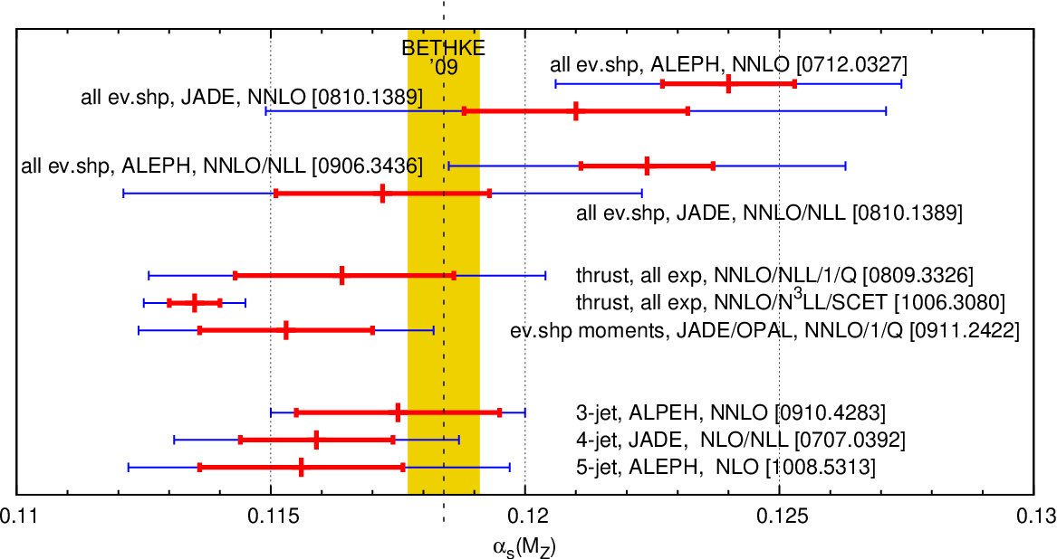
One possible workaround for the difficulties in treating hadronisation is simply not to correct for it and, perhaps, take its whole estimated impact as a systematic error. This was essentially the approach for the 5-jet rate extraction, and is potentially an option for jet rates because hadronisation tends to be smaller than for event-shape type observables. It may be of interest to investigate it also for the 3-jet rate, which seems to have a more convergent perturbative series than other observables and has been studied so far with only a subset of the data.
References
- [1] A. Gehrmann-De Ridder et al., Phys. Rev. Lett. 99 (2007) 132002; S. Weinzierl, Phys. Rev. Lett. 101 (2008) 162001.
- [2] S. Catani et al., Nucl. Phys. B407 (1993) 3; Y. L. Dokshitzer et al., JHEP 9801 (1998) 011; A. Banfi et al., JHEP 0201 (2002) 018.
- [3] T. Becher, M. D. Schwartz, JHEP 0807 (2008) 034; Y. -T. Chien, M. D. Schwartz JHEP 1008 (2010) 058.
- [4] Y. L. Dokshitzer, B. R. Webber, Phys. Lett. B404 (1997) 321-327.
- [5] R. Abbate et al., arXiv:1006.3080 [hep-ph].
- [6] G. P. Salam, D. Wicke, JHEP 0105 (2001) 061.
at NNLO(+NLLA) from (mainly) ALEPH data
Thomas Gehrmann
Institut für Theoretische Physik, Universität Zürich, CH-8057 Zürich, Switzerland
Event shapes and jet cross sections in annihilation were measured to a high accuracy at LEP and at previous colliders at lower energies. By comparing the data with the QCD description of these observables, it is possible to extract . During LEP times, only the next-to-leading order (NLO) QCD corrections (plus resummation of logarithmically enhanced terms) were available, and the theoretical uncertainty from missing higher order corrections was the dominant source of error on the extraction. With the recent calculation of next-to-next-to-leading order (NNLO) corrections to three-jet production and related event shapes [1], these data can be revisited in view of an improved determination of .
To compare with data, the perturbative NNLO prediction (or matched [2] to next-to-leading logarithmic resummation, NNLO+NLLA) is supplemented by quark mass effects (to NLO) and has to be corrected for hadronization effects. The standard procedure to estimate hadronization effects is to compare parton-level and hadron-level predictions obtained with multi-purpose (leading-order, leading-log) event generator programs for the observables. It has to be kept in mind that the hadronization models in these generators have been tuned extensively to precisely those LEP data sets that are analyzed now for the extraction.
With this procedure, has been determined from ALEPH [3], JADE [5] and OPAL [6] data, and the results are summarized in Table 1. Several important observations were made in these studies. First and foremost, inclusion of the NNLO corrections improves the mutual consistency of the extractions from the different shape variables. Compared to previous NLO studies, the theory error is lowered by almost a factor two. It increases when NLLA resummation is included, since this order of resummation is insufficient to match onto NNLO. A systematic tension between the ALEPH and OPAL extractions can be observed, which can be explained in part by different fit ranges and by the different treatment of quark mass effects.
| NNLO | ALEPH [3] | 0.12400.0008(stat)0.0010(exp)0.0011(had)0.0029(th) |
|---|---|---|
| OPAL [6] | 0.12010.0008(stat)0.0013(exp)0.0010(had)0.0024(th) | |
| NNLO | ALEPH [4] | 0.12240.0009(stat)0.0009(exp)0.0012(had)0.0035(th) |
| +NLLA | JADE [5] | 0.11720.0006(stat)0.0040(syst)0.0030(th) |
| OPAL [6] | 0.11890.0008(stat)0.0016(exp)0.0010(had)0.0036(th) |
Using hadronization corrections from more recent generators (HERWIG++, combined with POWHEG or MC@NLO), results are obtained that are substantially different from the PYTHIA values, and outside the band obtained from the different legacy generators. It may thus be fair to conclude that the the hadronization models in the generators may be over-tuned in order to compensate the shortcomings of the perturbative description in these programs and that the hadronization uncertainty on the extraction may be larger than assumed previously, and could actually be a dominant source of error. In order to circumvent this problem, one should either restrict to observables with small hadronization corrections (as for example jet rates) or turn to analytic hadronization models which allow a better order-by-order matching to the perturbative description of the event shape distributions. In two different studies, we pursued both approaches.
From analytic approaches to hadronization (e.g. dispersive model), it is known that the leading power corrections to most event shapes are of order . Among the standard set of shape variables, this power correction is absent only in (hadronization corrections to this variable start at ). The three-jet rate , which derives from is thus less sensitive to hadronization than the event shape distributions. We analyzed the LEP1 data on and extracted from the measurement at as [7]
Extractions at different jet resolution are highly correlated, and yield consistent results.
Hadronization corrections to the moments of event shape distributions are additive. The moments are therefore very well suited to to disentangle perturbative contributions from hadronization effects. After extending the dispersive model for hadronization corrections to match onto the perturbative NNLO expression, we used data on event shape moments from JADE and OPAL to determine and the hadronization parameter in a combined fit [8], yielding:
The hadronization corrections obtained in this approach are considerably larger than what is predicted by the legacy generators. The proper matching of the hadronization corrections onto the perturbative expression results in a considerable reduction of the theory uncertainty.
References
- [1] A. Gehrmann-De Ridder, T. Gehrmann, E. W. N. Glover and G. Heinrich, JHEP 0711 (2007) 058 [0710.0346]; JHEP 0712 (2007) 094 [0711.4711]; Phys. Rev. Lett. 100 (2008) 172001 [0802.0813]; S. Weinzierl, JHEP 0906 (2009) 041 [0904.1077]; Eur. Phys. J. C 71 (2011) 1565 [1011.6247].
- [2] T. Gehrmann, G. Luisoni and H. Stenzel, Phys. Lett. B 664 (2008) 265 [0803.0695].
- [3] G. Dissertori et al., JHEP 0802 (2008) 040 [0712.0327].
- [4] G. Dissertori et al., JHEP 0908 (2009) 036 [0906.3436].
- [5] S. Bethke et al. [JADE Collaboration], Eur. Phys. J. C 64 (2009) 351 [0810.1389].
- [6] G. Abbiendi et al. [OPAL Collaboration], [1101.1470].
- [7] G. Dissertori et al., Phys. Rev. Lett. 104 (2010) 072002 [0910.4283].
- [8] T. Gehrmann, M. Jaquier and G. Luisoni, Eur. Phys. J. C 67 (2010) 57 [0911.2422].
Next-to-Next-to-Leading Order and “Classic” Power Corrections
Bryan Webber
University of Cambridge, Cavendish Laboratory
Cambridge CB3 0HE, UK
Here I report on an analysis of the thrust distribution in annihilation, performed in collaboration with Richard Davison [5], in which the next-to-leading-logarithmic (NLL) resummed prediction of [2] was matched to the next-to-next-to-leading (NNLO) fixed-order results of [2], with non-perturbative effects included using the dispersive approach of [4].
To match the resummed and NNLO fixed-order predictions we use the log- matching scheme of [2]. The NLL resummed result is expressed as
| (1) |
where the coefficients are known and , being the kinematic limit for 5 partons, the maximum at NNLO. The terms with are subtracted and replaced by the full NNLO result for .
To include non-perturbative effects we note that the NLL resummed distribution has the form
| (2) |
where is the Laplace transform of the jet mass distribution. The idea of [4] is to subtract out the infrared contribution to this expression and substitute a non-perturbative contribution based on the assumption of a universal low-scale effective strong coupling . The NNLO perturbative contribution from the infrared region is
| (3) |
where is the renormalization scale, is the two-loop and the three-loop cusp anomalous dimension [5]. At the time of [5] was not known and we assumed , which is just equivalent to a change of renormalization scheme. This turns out to be a good guess ( versus for 5 flavours), although this term anyway has a negligible effect.
Assuming a universal low-scale coupling , the non-perturbative contribution from the region , where , i.e. , is
| (4) |
The change in the thrust distribution is given by the difference between (4) and (3), which we see is equivalent to a shift by an amount that is a power correction proportional to , modulo some logarithmic dependence if we take . Notice that the perturbative part (3) is the start of a divergent series in , representing the presence of an infrared renormalon. Thus universality of implies that the power correction should decrease as we include more terms in the perturbation series. In the fit of [5], the NNLO (order-) term does represent a significant decrease in the power correction, of 25% relative to NLO.
The resulting predictions have two free parameters, and . They were fitted to all the available thrust data in the c.m. energy range GeV. The fitting range was , giving a total of 430 data points. The best fit was at , , with . In view of the large contributions from certain data sets, the combined experimental statistical and systematic error was quoted in [5] for a of 14.6. For the experimental error is reduced by a factor of 3.4. On the other hand, the theoretical uncertainty was assessed by varying the renormalization scale by a factor of instead of the more usual factor of 2, which would double the theoretical error. With these revised error estimates, and taking into account loop corrections which give the ‘Milan factor’ [6], , the resulting parameter determinations were
| (5) |
It is a pleasure to thank the organizers for a very stimulating meeting and to acknowledge the support of a Leverhulme Emeritus Fellowship.
References
- [1]
R. A. Davison and B. R. Webber,
Eur. Phys. J. C 59 (2009) 13
[arXiv:0809.3326 [hep-ph]]; Erratum ibid. C 69 (2010) 341.
- [2]
S. Catani, L. Trentadue, G. Turnock and B. R. Webber,
Nucl. Phys. B 407, 3 (1993).
- [3]
A. Gehrmann-De Ridder, T. Gehrmann, E. W. N. Glover and G. Heinrich,
Phys. Rev. Lett. 99, 132002 (2007)
[arXiv:0707.1285 [hep-ph]];
JHEP 0711 (2007) 058
[arXiv:0710.0346 [hep-ph]];
JHEP 0712, 094 (2007)
[arXiv:0711.4711 [hep-ph]];
S. Weinzierl,
Phys. Rev. Lett. 101, 162001 (2008)
[arXiv:0807.3241 [hep-ph]].
- [4]
Y. L. Dokshitzer and B. R. Webber,
Phys. Lett. B 352, 451 (1995)
[arXiv:hep-ph/9504219];
Phys. Lett. B 404, 321 (1997)
[arXiv:hep-ph/9704298];
Y. L. Dokshitzer, G. Marchesini and B. R. Webber,
Nucl. Phys. B 469, 93 (1996)
[arXiv:hep-ph/9512336].
- [5]
T. Becher and M. Neubert,
Phys. Rev. Lett. 102, 162001 (2009)
[arXiv:0901.0722 [hep-ph]];
JHEP 0906, 081 (2009)
[arXiv:0903.1126 [hep-ph]];
E. Gardi and L. Magnea,
JHEP 0903, 079 (2009)
[arXiv:0901.1091 [hep-ph]].
- [6]
Y. L. Dokshitzer, A. Lucenti, G. Marchesini and G. P. Salam,
JHEP 9805, 003 (1998)
[arXiv:hep-ph/9802381].
from Thrust at N3LL with Power Corrections
R. Abbate, A.H. Hoang, V. Mateu, M. Fickinger, M. Schwartz, I.W. Stewart
Center for Theoretical Physics, Massachusetts Institute of
Technology, Cambridge, MA 02139, U.S.A.
Max-Planck-Institut für Physik (Werner-Heisenberg-Institut), Föhringer Ring 6, D-80805 München, Germany.
Instituto de Física Corpuscular, UVEG - CSCIC, Apartado de Correos 22085,
E-46071, Valencia, Spain.
Center for the Fundamental Laws of Nature, Harvard University, Cambridge, MA 02138, U.S.A.
Department of Physics, University of Arizona, Tucson, AZ 85721, U.S.A.
We perform a global fit of data for the thrust event shape at energies between and GeV [1]. We will consider the results with six stages of theoretical improvements:
- 1.
- 2.
- 3.
Profile functions (-dependent scales , , , ) that account for the multijet boundary condition, which ensures fixed-order results are used in the far tail region.
- 4.
Description of nonperturbative effects with field theory and a fit to a single nonperturbative matrix element of Wilson lines . ’s uncertainty dominates other OPE terms in the tail region, and its Wilson coefficient is included with N3LL + accuracy.
- 5.
Switching from to an R-scheme to define . This ensures and the perturbative cross-section are free of renormalon ambiguities. An RGE is used to sum large logarithms in the perturbative renormalon subtractions. The fit gives to .
- 6.
QED final state corrections at and NNLL (counting ); bottom mass corrections are included using a factorization theorem with log resummation; axial-singlet terms arising from the large top-bottom mass splitting.
We fit simultaneously for and in the tail region of the thrust distributions (our default 487 bin dataset has to ). For fixed Q there is a strong degeneracy between and . It is lifted by the global fit with different Q values. To estimate perturbative uncertainties we performed a point random scan over 12 parameters, refitting for each point. This accounts for theory uncertainty from higher orders via varying scales, statistical theory errors, and three unknown perturbative coefficients. We observe very good convergence when increasing the orders in perturbation theory [1], and achieve at stage 6. The results are shown in Fig. 1, including a comparison with [3] and [4] at the appropriate stages. For the global fit at stage 2 our random scan uses the variations of [4]. Stage 3 yields a result midway between 1 and 2.
The most dramatic effect is the decrease to from adding the nonperturbative fit parameter at stage 4. The size of this shift is consistent with a back of the envelope estimate based on data [1]. The field theory treatment is in sharp contrast with the traditional method of estimating nonperturbative effects employing Monte Carlo generators (MC) (used also in [3] and [4]). MC has less perturbative accuracy than level 1, and its tune parameters unavoidable include both nonperturbative and higher order perturbative effects, leading to a double counting in the MC estimate. At the Z-scale the Pythia tune has a very small power correction, inconsistent with our determination, and hence cannot be used for high precision determinations. In [5] a global fit was performed at NLL respectively with the effective coupling model to treat nonperturbative effects. They find consistent with our stage 2, 4, 5, 6 fits. This model agrees with the parametrics of the OPE in the tail region and has renormalon subtractions. Advantage of our approach are that the power correction is defined as a field theory matrix element, one can include subleading OPE terms, and sum large logs in the subtractions. Our final result with all sources of uncertainty is shown in the box in Fig. 1.
Given the desired precision, an interesting issue is to assess the most appropriate way of computing the binned theory distribution. Two approaches being used are:
| (1) |
where and are jet and soft scales depending on . They are equivalent at a given order in resummed perturbation theory, but differ by noticeable amounts from included higher order terms [1]. In particular, gives an uncertainty estimate that is designed for comparison to cumulant data, and (b) is sensitive to contributions from below the bin . The uncertainties in are designed for distributions and hence (a) is best suited for the bins. (a) was used in [1], while (b) was used in classical resummation analyses and [4]. At stage 2 this issue is small for thrust, and only becomes noticeable at stage 3. For the Heavy Jet Mass (HJM) event shape it is already noticeable at stage 2. The stage 2 thrust and HJM results in Refs. [4] use (b) and yield: vs . Using (a) yields consistent values for thrust and HJM: vs , resolving the apparent discrepancy in central values.

Work supported in part by the European Community’s Marie-Curie Research Training Network PITN-GA-2010-264564
(LHCphenOnet), and by the Offices of Nuclear and Particle Physics of the U. S. Department of Energy under grants
FG02-94ER40818, DE-FG02-06ER41449 and DE-SC003916. VM has been partially supported by a Marie Curie Fellowship
under contract PIOF-GA-2009-251174. IS was also supported in part by a Friedrich Wilhelm Bessel award from the Alexander.
von Humboldt foundation. Preprint number: MIT-CTP 4301
References
- [1]
R. Abbate, M. Fickinger, A. H. Hoang, V. Mateu, I. W. Stewart,
Phys. Rev. D83, 074021 (2011).
[arXiv:1006.3080 [hep-ph]].
- [2] A. Gehrmann-De Ridder et al, Phys. Rev. Lett. 99, 132002 (2007); S. Weinzierl, Phys. Rev. D 80 (2009) 094018.
- [3]
G. Dissertori et al,
JHEP 0802 (2008) 040.
- [4]
T. Becher and M. D. Schwartz,
JHEP 0807, 034 (2008);
Y. T. Chien and M. D. Schwartz,
JHEP 1008 (2010) 058.
- [5]
R. A. Davison and B. R. Webber,
Eur. Phys. J. C 59 (2009) 13.
from five-jet observables at LEP
Giulia Zanderighi
Rudolf Peierls Centre for Theoretical Physics, 1 Keble Road, OX1 3PN, Oxford, UK
Jet observables represent powerful tools to measure the strength of the strong interactions, encoded in . The more jets are present in the final state, the stronger is the dependence of the relevant observables on . At LEP the highest exclusive multiplicity measured is five. However, since five-jet events could be described only at leading order (LO) in QCD, the theoretical uncertainty was too large to extract a competitive value for . We recently computed the next-to-leading (NLO) QCD corrections to five-jet events [1] using -dimensional unitarity for the one-loop calculation [2] and Madgraph and MadFKS for the real radiation, subtraction, and phase-space integration [3]. We consider two observables: the five-jet resolution parameter, , and the five-jet rate, . Their perturbative distributions start at , and are therefore very sensitive to the value of . We find that, once NLO corrections are included, ALEPH data is described well by perturbative QCD if the world-average of is used as input of the theoretical prediction. Furthermore, theoretical uncertainties are reduced from at LO to at NLO. One can then turn this around and use the NLO calculation for a novel extraction of using ALEPH data. Before this can be done, one needs to address how non-perturbative hadronization corrections can be accounted for. Traditionally, they are extracted using parton showers such as Herwig of Pythia. We find however that, if this is done, the hadronization corrections are very large () and generator dependent. We therefore use the Sherpa event generator [4] with its default cluster model [5] to extract hadronization effects. Sherpa implements the five-jet LO matrix element exactly, therefore hadronization corrections are less contaminated by missing perturbative effects. When this is done, we find smaller hadronization corrections (). We also observe that while the hadronization corrections per se are not negligible, they have a very small effect on the extraction of at LEP I, therefore we neglect hadronization corrections at LEP II.
In order to extract we consider each bin of and at a given energy as an observable that can be used to measure by solving the equation , where is the perturbative theoretical prediction, is the hadronization correction and is the experimental measurement. From each bin we obtain a central value of with corresponding errors
| (1) |
The systematic and statistical errors are obtained by solving the same equation with , the perturbative error is obtained by varying the default scale ( by a factor two up and down, and the hadronization error is obtained by solving the same equation using the Lund hadronization model [6]. We take the fit range as large as possible, where our computation is reliable and data are good enough. We then vary the range to estimate a fit range error. Full details about the fit ranges and the fitting procedure are given in [1]. The result of this procedure it a set of values of that need to be combined. To do this we define a covariance matrix as the sum of individual covariance matrices with
| (2) |
where describes the correlation. We assumed that statistical errors are uncorrelated at different energies. At a given energy we take bins as uncorrelated, bins as fully correlated and and to be correlated for . Systematic errors are taken as fully correlated at fixed energy, but uncorrelated at different energies. Perturbative errors are taken to be fully correlated for all observables and energies, except for the LEP I/LEP II correlation that we neglect. Finally, hadronization errors are assumed to be fully correlated. We then compute the weights and use them to obtain the estimate of the average of the strong coupling constant and of its error
| (3) |
We obtain the value of from five-jets (a breakdown of the errors is displayed in Fig. 1)
| (4) |
This value is compatible with the current world average, but on its lower side.
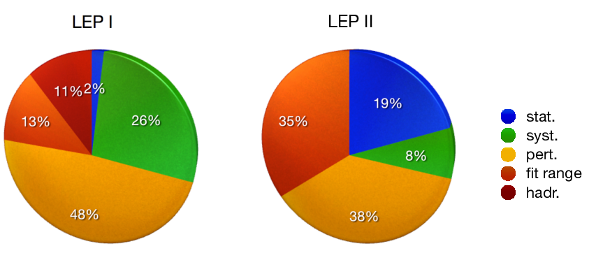
References
- [1] R. Frederix, S. Frixione, K. Melnikov, G. Zanderighi, JHEP 1011 (2010) 050.
- [2] R. K. Ellis, W. T. Giele and Z. Kunszt, JHEP 0803, 003 (2008); W. T. Giele, Z. Kunszt and K. Melnikov, JHEP 0804, 049 (2008) R. K. Ellis et al. JHEP 0901, 012 (2009).
- [3] J. Alwall et al. JHEP 0709, 028 (2007); S. Frixione, Z. Kunszt, A. Signer, Nucl.Phys. B 467, 399 (1996); R. Frederix et al. JHEP 0910, 003 (2009).
- [4] T. Gleisberg et al., JHEP 0902 (2009) 007.
- [5] J. C. Winter, F. Krauss, and G. Soff, Eur.Phys.J. C36 (2004) 381–395.
- [6] B. Andersson, et al., Phys.Rept. 97 (1983) 31–145.
Jet and Event Shape Observables at LHC
Klaus Rabbertz
Institut für Experimentelle Kernphysik, KIT, Postfach 6980, D-76128 Karlsruhe, Germany
During the first, very successful year 2010 of LHC operation, which saw an increase in instantaneous luminosity by a factor of , an excellent performance of the LHC experiments ATLAS and CMS has been observed. The achieved understanding in detector operation and behaviour has lead to uncertainties of the order of on the luminosity, – on the jet energy scale and about – on the jet energy resolution depending on experiment and phase space. With respect to their impact on QCD measurements three general analysis strategies can be differentiated: Absolute measurements like the inclusive jet , shape measurements like jet angular variables and event shapes, or ratios of cross sections. The latter two exhibit much smaller experimental uncertainties due to cancellation effects and are, at least in the beginning, better suited for precise QCD studies in order to constrain parton distribution functions (PDFs) and/or determine the strong coupling constant . The total experimental uncertainties on the jet cross sections currently are of the order of to for transverse momenta larger than GeV while theoretical uncertainties from the PDFs, the renormalization and factorization scales, and non-perturbative corrections amount to to . With further improvements and much more data to come the jet cross sections are very promising for the future. In the following, some aspects of a shape measurement, the azimuthal decorrelation , and the 3-jet ratio will be discussed.
Azimuthal decorrelations , recently published for LHC data by CMS and ATLAS [1], are normalized to the total dijet cross section eliminating luminosity uncertainties. They are a direct measure of additional activity like a radiated third jet in comparison to a normal dijet event perfectly balanced in transverse momentum. Restricting the observation to differences in azimuthal angle between the leading two jets reduces significantly uncertainties due to the jet energy scale and resolutions. In case of balanced dijet events the azimuthal angles between the leading jets are completely correlated to give distances of . Additional radiation of any of the two jets decrease this distance where the extent to which this is possible depends on the jet multiplicity as demonstrated e.g. in Fig. 1 of the ATLAS analysis in [1]. Comparisons to pQCD at NLO are possible in the range with NLOJet++ [4] providing the required 3-parton and 4-parton final states. Below mostly final states with four or more partons contribute such that the result of NLOJet++ effectively becomes LO only. This can also be seen by an associated increase of the scale uncertainties. At the 3- and 4-parton final states need to be complemented by the 2-parton ones requiring 2-loop corrections for a complete NNLO result which is not available as of today. This demonstrates that azimuthal decorrelations are a precisely measurable QCD observable providing a lot of information on multijet production. Redefining the azimuthal distance to such that balanced dijets have this quantity can also be considered an event shape for which resummed predictions are conceivable [2]. Azimuthal decorrelations can also be investigated for leading particles.
Following a publication of D0, preliminary results by ATLAS and CMS [3] are reported for the inclusive 3- to 2-jet ratio versus the scalar sum of all transverse jet momenta . The suggested study, however, is far from optimal with respect to comparisons to pQCD. First of all, the LO prediction including the scale uncertainty as shown in Fig. 1 left as upper red hatched band is unreliable and gives unphysical values larger than one. The NLO presented in blue looks more reasonable and is not far off the CMS data, but the associated scale uncertainties are not much smaller with respect to LO. This points to a bad convergence of the perturbative series. In fact, ratios of where jets with GeV are counted even for leading jet momenta of TeV are not representative for hard processes with probabilities related to at high scales. For that purpose it would be better to require a minimal hardness of third jets of e.g. a certain percentage like of the average transverse momentum of the two leading jets. An example calculation performed with NLOJet++ in the fastNLO framework [5] for such an event selection is presented in Fig. 1 right leading to reasonable predictions already at LO and larger reductions of the scale uncertainties at NLO at least at high . The abundant production of jets at highest transverse momenta at the LHC will enable many new precision tests of perturbative QCD in the near future.


References
- [1]
D0 Collaboration, Phys.Rev.Lett. 86 (2001) 1955;
CMS Collaboration, accepted by Phys.Rev.Lett., arXiv:1101.5029 (2011);
ATLAS Collaboration, submitted to Phys.Rev.Lett., arXiv:1102.2696 (2011). - [2] A. Banfi, arXiv:0906.4958 (2009).
- [3]
ATLAS Collaboration, ATLAS Conference Note ATLAS-CONF-2010-084 (2010);
CMS Collaboration, CMS Physics Analysis Summary CMS-PAS-QCD-10-012 (2010). - [4] Z. Nagy, Phys.Rev.Lett. 88 (2002) 122003; Z. Nagy, Phys.Rev. D68 (2003) 094002.
- [5] T. Kluge, K. Rabbertz and M. Wobisch, in proceedings DIS 2006, Tsukuba, Japan, hep-ph/0609285 (2006).
MC tuning with Professor
Andy Buckley (University of Edinburgh), Hendrik Hoeth (IPPP Durham), Heiko Lacker (HU Berlin) , Holger Schulz (HU Berlin), Jan Eike von Seggern (DESY Hamburg)
Humboldt-Universität zu Berlin, Institut für Physik, Newtonstr. 15, 12437 Berlin, Germany
holger.schulz@physik.hu-berlin.de
Monte Carlo simulations of high energy physics (and particularly QCD) processes rely on phenomenological assumptions for regimes where perturbation theory does not apply. Of particular interest for extractions from event-shape data are hadronisation-effects for which two kind of models are available. On the one hand cluster based models, e.g. in the codes of Herwig and Sherpa, and the Lund-string model as it is implemented in the Pythia event generator.
Both types have in common that a large number of tunable phenomenological parameters are necessary to achieve agreement with data and therefore predictive power. The task of tuning such generator parameters can be cumbersome if done by hand due to the high dimensionality of the parameter-space and the large number of observables that need to be studied for changes due to parameter-shifts.
The Professor[1] tuning-tool which tries to address the aforementioned problems was presented. It is based on the idea of calculating bin-wise parameterisations of the generator response to shifts in a certain parameter space and a subsequent numerical minimisation of a simple goodness-of-fit measure defined between the parameterisation and corresponding experimental data.
Furthermore, special applications of Professor have been introduced that exploit the statistical nature of the tool such as the quantification of tuning uncertainties as well as the calculation of so-called “Eigentunes”, a set of parameter points on the -contour of the valley that are therefore representative for allowed tuning variations within data-uncertainty (Fig. 1).
Further uses of the parameterisation like calculating the sensitivity of observables to shifts in parameter space and an interactive Monte Carlo simulator (“prof-I”) have been presented as well.


On request of the organisers, a quick study on a possible dependence of a hadronisation tune, namely the Pythia6 tune pro-[1], has been performed. This most recent hadronisation tuning was obtained from tuning the generator parameters to event shape data on the Z-pole. This is in large parts due to the fact that the development of Professor and tunings obtained with it are closely linked to the development of Rivet[2], an application designed for generator independent validation by means of built-in analyses that mimic published studies of collider experiments. By the time of the workshop only event shape data from the LEP I and II experiments was available in Rivet. An outcome of the workshop was the implementation of event shape studies of the PETRA experiments JADE and TASSO at energies between 14 and 44 GeV[,] which allowed to study the low-energy behaviour of the tune after the workshop.
Equipped with event shape data and corresponding Rivet analyses at energies between 14 and 209 GeV[,,], the per-bin goodness-of-fit of the tune pro- and data could be studied for the Thrust, C-Parameter and 2-jet-resolution parameter, , as a function of . The result is given in Fig. 1.
The data seems to suggest that Pythia6’s hadronisation model or at least the selected tuning is not capable of describing the data at all, especially low energies. Further studies should include more data, preferably at low energies. It may be fruitful to attempt a retuning to all available event shape data simultaneously to check if the available hadronisation models are in fact not universal.
We would like to thank Stefan Kluth for the discussions that lead to the implementation of the JADE analysis in Rivet.
References
- [1] A. Buckley, H. Hoeth, H. Lacker, H. Schulz and J. E. von Seggern, “Systematic event generator tuning for the LHC,” Eur. Phys. J. C 65 (2010) 331
- [2] A. Buckley et al., “Rivet user manual,” arXiv:1003.0694 [hep-ph].
- [3] P. A. Movilla Fernandez, O. Biebel, S. Bethke, S. Kluth and P. Pfeifenschneider [JADE Collaboration], “A study of event shapes and determinations of alpha(s) using data of e+ e- annihilations at s**(1/2) = 22-GeV to 44-GeV,” Eur. Phys. J. C 1 (1998) 461
- [4] W. Braunschweig et al. [ TASSO Collaboration ], “GLOBAL JET PROPERTIES AT 14-GeV TO 44-GeV CENTER-OF-MASS ENERGY IN e+ e- ANNIHILATION,” Z. Phys. C47 (1990) 187-198.
- [5] A. Heister et al. [ALEPH Collaboration], “Studies of QCD at e+ e- centre-of-mass energies between 91-GeV and 209-GeV,” Eur. Phys. J. C 35 (2004) 457.
from event shapes in : Experimental issues
and combination of results
Stefan Kluth
MPI für Physik, Föhringer Ring 6, 80805 München
| PETRA/JADE | LEP1 | LEP2 | |
| Rad. return | cuts on 4-momentum balance | n.a. | cuts on 4-momentum balance, cuts on |
| pairs | , reject 1- vs. 3-prong events | ||
| 2 events | cuts on 4-momentum sum | ||
| 4-fermion events | n.a. | “4-jet event shape” cuts | |
Detector corrections take account of limited acceptance and resolution of the experiments, and of QED initial state radiation (ISR) effects, and are performed using MC based unfolding of the measured distributions. Table 2 gives an overview over the treatment of various experimental effects by the LEP experiments, the selection efficients and final background fractions, and the resulting experimental systematic uncertainties. The uncertainties are average values and can change significantly within a given distribution. The LEP1 experimental systematics are still to be matched by theory while the LEP2 experimental systematics have been reached by recent theory uncertainties. The JADE data have experimental systematics varying between 0.7 and 4%.
| ALEPH | DELPHI | L3 | OPAL | |
| Rad. return | find EM jets, force remaining event in 2 jets | kin. fit for jet and possible missing energies along beam | cuts on , , , | find isolated , force remaining event into 4 jets, kin. fit for for jet and possible missing energies along beam |
| 4-fermion bkg | force 4 jets, cut on and | 2d cut on vs. | force 4 jets, cuts on , , , | cut on likelihood from partial NLO QCD and EW ME, , Sphericity |
| LEP1 exp. syst. | % (exp. corr.) | 1.6% | 1.5% (exp. corr.) | % (exp. corr.) |
| LEP1 | – | 84.5% | 88.5% | |
| LEP2 exp. syst. | % (non-rad.) | % | 1.0-2.5% (non-rad or 4-f) | 0.8-4% (4-f cuts) |
| LEP2 | – | % | ||
| LEP2 | – | 5-14% | 20% | 2-6% |
| b-Quarks | NLO massive ME, no corr. syst. | udsc/udscb had. corr., 20% syst. | NLO massive ME | neglect, udsc had. corr. syst. |
Combinations of NLO+NLLA results from the analysis of event shape observables were performed by the collaborations using procedures assuming normal distributions for all uncertainties. Values of are always evolved to a common scale before combining them. The observables are statistically correlated and have correlated systematic uncertainties. ALEPH, DELPHI and OPAL use a common method while L3 calculates unweighted averages. In the common method experimental uncertainties are taken as partially correlated (see below) within an experiment and as uncorrelated between experiments. Hadronisation and theory systematics are taken as uncorrelated, and the combination procedures are repeated for different hadronisation models or theory parameters such as the renormalisation scale. Statistical correlations within or between observable distributions are measured or obtained from MC simulations. For correlations of systematic uncertainties models are employed: i) no correlation (), ii) partial correlation ( or iii) full correlation (). In [6] a combination of all NLO+NLLA results from LEP and JADE using the common method is shown. However, the recent analyses of LEP or JADE data using NNLO(+NLLA) calculations have not yet been combined.
References
- [1] A. Heister et al. (ALEPH coll.), Eur. Phys. J. C35 (2004) 457
- [2] J. Abdallah, et al. (DELPHI coll.), Eur. Phys. J. C29 (2003) 285
- [3] P. Archard et al. (L3 coll.), Phys. Rept. 399 (2004) 71
- [4] G. Abbiendi et al. (OPAL coll.), Eur. Phys. J. C40 (2005) 287
- [5] S. Bethke et al. (JADE coll.), Eur. Phys. J. C64 (2009) 351
- [6] S. Kluth, Rept. Prog. Phys. 69 (2006) 1771
Lattice QCD Calculations and
Andreas S. Kronfeld
Theoretical Physics Department, Fermi National Accelerator Laboratory,
Batavia, Illinois, USA
Lattice gauge theory provides a mathematically rigorous definition of quantum field theories, such as QCD, encompassing the perturbative and nonperturbative regimes [1]. In principle, it is ideally suited for the determination of and the quark masses, which are the irreducible parameters of QCD. In practice, the most productive approach to lattice QCD has been computational, evaluating the functional integrals of quantum field theory with Monte Carlo methods and importance sampling.
The first such calculations were marred by the omission of sea quarks, often called the “quenched approximation.” The sea quarks are the most computationally demanding part of the calculations and, in the early days, a lack of computer power made the quenched approximation a necessary compromise. Quenched QCD calculations are on a footing similar to models of nonperturbative QCD. Consequently, the first lattice-QCD determinations of required a model-dependent corrections for the omitted sea. In particular, potential models could be used to patch up the mass splittings in charmonium and bottomonium [2].
Since the start of the new millenium, however, lattice QCD simulations with 2+1 flavors of sea quarks have become routine [3]. The notation “2+1” implies one sea quark tuned to the strange quark and two taken with masses as small as possible, for (degenerate) up and down. The physical limit is reached by extrapolating numerical data, guided by chiral perturbation theory. More recently, the first simulations obviating this extrapolation have been carried out [,,] (though not used for —yet). Furthermore, at least two collaborations have begun wide-ranging programs of lattice-QCD calculations of 2+1+1 sea quarks—adding the charmed sea to the rest [,]. Thanks to these developments, lattice QCD now plays an increasingly important role in many areas, for example, flavor physics [8].
Dating back to Ref. [2], many summaries of perturbative QCD still identify from lattice QCD with the quarkonium splittings. This is outdated. In fact, the possibilities are much broader and share many features with determinations of from high-energy scattering or the decays of heavy particles. To explain this perspective, let us list the ingredients needed to determine . One needs
- 1.
A dimensionless quantity, , sensitive to QCD at a (range of) short distance(s), ; if is not dimensionless, one can use to make it so; then asymptotic freedom implies , where is a specific scale choice for scheme with , and the power depends on the observable .
- 2.
A theoretical framework—or at least a notion—to separate short-distance scales from and other long-distance scales.
- 3.
A perturbative series for the short-distance contribution , certainly to NLO and preferably to higher order, and summing logarithms of scale ratios.
- 4.
Measurements of over a range of large enough to control the power-law effects, denoted in item 1.
- 5.
Control of non-QCD physics at scales probed by (e.g., electroweak or new physics).
- 6.
A measurement of : usually a calibration, in contrast to event counting for .
It is worth emphasizing that the whole procedure can be thought of as dimensionless until the last step, where the energy calibration of the calorimeters (high-energy scattering) or the -lepton mass ( decays) is input.
In lattice QCD, an evaluation of a functional integral replaces the measurement of . One is assured that non-QCD physics does not enter, but, in practice, issues like unphysical quark masses and nonzero lattice spacing play an analogous role. We know how to control these effects, i.e., how to distill them into an error bar. Many choices of are possible, each with strengths and weaknesses. The dimensionless suite of lattice calculations becomes dimensionful when converting from lattice units to GeV—this precisely means deducing the scale to which the corresponds (here labels the scheme chosen in the lattice calculation). Since lattice QCD with 2+1 sea quarks reproduces a wide variety of masses, mass splittings, and decay constants, the quantity used to convert units is no longer crucial [3], and the error on the conversion is subdominant when propagated to .
The table compiles several recent determinations of from lattice QCD with 2, 2+1, or 2+1+1 flavors. Near-term global averages should consider using those set in bold, after some dialogue with the authors to ensure a consensus between reviewers and authors of the completeness and meaning of the error budgets. The others either are superseded [,], are a re-analysis of a bold entry [11], omit the possibly large uncertainty from quenching the strange sea [16], or are not yet complete [17]. Longer-term global averages of will have more results from lattice QCD to choose from.
| range | sea | Ref. | ||||
|---|---|---|---|---|---|---|
| 0.1170(12) | 3 | [9] | ||||
| 0.1183(8) | Wilson loops | 7 | NNLO | 2+1 | [10] | |
| 0.1192(11) | 7 | [11] | ||||
| 0.1174(12) | quarkonium | 1–2 | NNLO | 2+1 | [12] | |
| 0.1183(7) | correlators | 3–6 | NNLO | 2+1 | [1] | |
| 0.1181(3) | Adler function | 5 | NNLO⋆ | 2+1 overlap | [2] | |
| 0.1205(8)(5) | “QCD in a can” | 80 | 2+1 Wilson | [15] | ||
| 0.1000(16)† | aka Schrödinger | 270 | asymptotic | 2 Wilson | [16] | |
| 0.1 ( ) | functional | 1000 | 2+1+1 Wilson | [17] |
⋆ The Adler function’s is known to N3LO, but Ref. [2]’s analysis is NNLO.
† This entry gives , obtained from Ref. [16]’s with
fm and Eq. (9.5) of the 2006 PDG.
References
- [1] K. G. Wilson, Phys. Rev. D 10 (1974) 2445.
- [2] A. X. El-Khadra et al., Phys. Rev. Lett. 69 (1992) 729.
- [3] C. T. H. Davies et al. [HPQCD, MILC, and Fermilab Lattice], Phys. Rev. Lett. 92 (2004) 022001 [hep-lat/0304004].
- [4] S. Aoki et al. [PACS-CS], Phys. Rev. D 81 (2010) 074503 [arXiv:0911.2561].
- [5] A. Bazavov et al. [MILC], Phys. Rev. D 82 (2010) 074501 [arXiv:1004.0342].
- [6] S. Dürr et al. [BMW], arXiv:1011.2711 [hep-lat].
- [7] R. Baron et al. [ETM], JHEP 1008 (2010) 097 [arXiv:0911.5061].
- [8] M. Antonelli et al., Phys. Rept. 494 (2010) 197 [arXiv:0907.5386].
- [9] Q. Mason et al. [HPQCD], Phys. Rev. Lett. 95 (2005) 052002 [hep-lat/0503005].
- [10] C. T. H. Davies et al. [HPQCD], Phys. Rev. D 78 (2008) 114507 [arXiv:0807.1687].
- [11] K. Maltman et al., Phys. Rev. D 78 (2008) 114504 [arXiv:0807.2020].
- [12] I. Allison et al. [HPQCD], Phys. Rev. D 78 (2008) 054513 [arXiv:0805.2999].
- [13] C. McNeile et al. [HPQCD], Phys. Rev. D 82 (2010) 034512 [arXiv:1004.4285].
- [14] E. Shintani et al. [JLQCD], Phys. Rev. D 82 (2010) 074505 [arXiv:1002.0371].
- [15] S. Aoki et al. [PACS-CS], JHEP 0910 (2009) 053 [arXiv:0906.3906].
- [16] M. Della Morte et al. [Alpha], Nucl. Phys. B 713 (2005) 378-406 [hep-lat/0411025].
- [17] R. Sommer, F. Tekin, and U. Wolff [Alpha], PoS LATTICE2010 (2010) 241 [arXiv:1011.2332].
HPQCD: from Lattice QCD
G. Peter Lepage (for HPQCD)
Laboratory for Elementary-Particle Physics
Cornell University, Ithaca, New York 14853, USA
The HPQCD collaboration has been using lattice QCD simulations for more than a decade to determine the QCD coupling from experimental data for hadron masses. That history, which has produced consistent results over time, is summarized in the following:
![[Uncaptioned image]](1110.0016v3/lepage-history.png)
HPQCD now uses two very different approaches (red and blue in the plot), with very different systematic errors, for extracting the coupling [1]. These give almost identical results for the coupling: and 0.1183(7).
The only experimental inputs to a QCD simulation are the small number of well-measured hadronic quantities (, …) used to tune the bare quark masses and bare QCD charge in the action. Typically simulations are done for a variety of light-quark masses and lattice spacings (and volumes) in order to extrapolate away lattice artifacts. Extrapolated simulation results should agree with continuum QCD to within simulation and extrapolation errors (of order 1% in many, many tests); there are no free parameters after tuning. We determine by “measuring” various short-distance quantities (nonperturbatively) in the simulation, and comparing with the corresponding perturbative expansions: , where the are computed using Feynman perturbation theory.
Small Wilson loops are the easiest short-distance quantities to measure in a simulation. Five-digit precision is routine and the loops are very ultraviolet, and therefore also highly perturbative provided (lattice UV cutoff) is large [2]. HPQCD used 22 different combinations of 8 small loops and the bare coupling, for each of 12 different combinations of - quark mass and lattice spacing ( GeV), to extract 22 different values for the coupling. Perturbation theory was calculated, through third order, using lattice QCD perturbation theory, which includes lattice-spacing artifacts to all orders in the lattice spacing. Fourth and higher orders were estimated by comparing results from different lattice spacings (since ). Nonperturbative effects, such as condensate contributions, were included, and can vary by factors of 100 or more between different quantities. Nevertheless all 22 quantities agree to within errors with [1].
To test HPQCD’s error estimates, we pretend that perturbation theory is known only to first or second order but otherwise use the same analysis, including the estimation of higher-order perturbation theory by comparing different lattice spacings. Values for from each of the 22 quantities are shown in the following figure:
![[Uncaptioned image]](1110.0016v3/lepage-orders.png)
The gray bars show the final result, 0.1184(6), from the full analysis. The first, second and third order analyses agree to within their errors of order 0.0092, 0.0018 and 0.0006, respectively. Convergence is excellent and the error estimates robust.
The second approach for determining used by HPQCD is to measure moments of current-current correlators of the form where and is a heavy quark ( or ). Low-order moments are short-distance and therefore perturbative. They also are renormalized quantities, unlike Wilson loops, and so should agree with continuum QCD results when extrapolated to zero lattice spacing. HPQCD analyzed four moments at approximately 8 different values of the heavy-quark mass between and and 5 different lattice spacings. The analysis produced very accurate values for the coupling, , and also for the and masses [1]. The masses agree with results from pure continuum analyses of moments to within about 0.5% — an important check on the lattice analysis.
The agreement between HPQCD’s Wilson-loop and current-current correlator determinations of the coupling is perhaps the most compelling check on each method since the systematic errors are very different in the two cases. Many additional tests are discussed in [1].
References
- [1]
C. McNeile et al.,
Phys. Rev. D82 (2010) 034512.
[arXiv:1004.4285 [hep-lat]]. See also C. T. H. Davies et al.,
Phys. Rev. D78 (2008) 114507.
[arXiv:0807.1687 [hep-lat]].
- [2]
G. P. Lepage, P. B. Mackenzie,
Phys. Rev. D48 (1993) 2250-2264.
[hep-lat/9209022].
from PACS-CS
Sinya AOKI
Graduate School of Pure and Applied Sciences, University of Tsukuba, Tukuba, Ibaraki 305-8571, Japan, and Center for Computational Sciences, University of Tsukuba, Tukuba, Ibaraki 305-8577, Japan
We evaluate the running coupling constant for 2+1 flavors in lattice QCD simulations[1]. The Schrödinger Functional(SF) scheme is employed as the intermediate scheme to carry out non-perturbative running from the low energy region, where physical scale is introduced as , to deep in the higher energy perturbative region, where a conversion to the scheme is safely performed: For 3 flavors we have
| (1) | |||||
| (2) |
where is the running coupling constant in the SF scheme at the box size , and the 3-loop beta function in the SF scheme with
| (3) |
and the universal . The SF scheme is the non-perturbative scheme whose scale is determined solely by the box size without any other scales. The continuum() limit can be taken in this scheme where is the lattice spacing.
To convert to , we first run down at using the 4-loop beta function and then convert it to at using the 3-loop matching. Next we run up and convert it to at . We finally run up at .
The low energy scale should be determined by other simulations. We use the scale determination in QCD simulations at three lattice spacings by CP-PACS/JLQCD collaborations[2] whose up-down quark mass covers a rather heavy region corresponding to .
Our final results in the continuum limit are
| (4) | |||||
| (5) |
where the first error is statistical, the second one is systematic due to the perturbative matching at , while the last is due to the continuum extrapolation.
References
- [1]
S. Aoki et al. (PACS-CS collaboration),
JHEP 0910 (2009) 053.
- [2]
T. Ishikawa et al. (CP-PACS/JLQCD collaborations),
Phys. Rev. D78 (2008) 011502.
Alpha_s from JLQCD
Shoji Hashimoto
High Energy Accelerator Research Organization (KEK), Tsukuba 305-0801, Japan.
Lattice determination of is performed using some perturbative (or short distance) quantity calculated non-perturbatively on the lattice. Typical examples are the heavy quark potential at short distances and small Wilson loops. One could also consider the vector current correlator in the space-like region. Perturbative expansion for this quantity is available to (!) in the continuum theory, and the long-distance contribution is theoretically well understood using the Operator Product Expansion (OPE). We propose to use this quantity for the determination of [1]. The correlator itself is ultraviolet divergent, but its derivative in terms of is finite and unambiguously calculable also in lattice QCD.
There are potential sources of systematic errors due to (i) discretization effect that could be significant at short distances, (ii) truncation error of the perturbative expansion, (iii) uncertainty of lattice spacing. These are studied and found to be under good control. Our result obtained using our lattices generated with 2+1-flavors of dynamical overlap fermion is [2]. The error is dominated by the uncertainty of lattice spacing, that is significant in our simulation on a relatively small and coarse lattice.
References
- [1] E. Shintani et al. [ JLQCD and TWQCD Collaborations ], Phys. Rev. D79 (2009) 074510. [arXiv:0807.0556 [hep-lat]].
- [2] E. Shintani, S. Aoki, H. Fukaya, S. Hashimoto, T. Kaneko, T. Onogi, N. Yamada, Phys. Rev. D82 (2010) 074505. [arXiv:1002.0371 [hep-lat]].
from the ALPHA collaboration
Rainer Sommer for the collboration
NIC, DESY, Platanenallee 6, 15738 Zeuthen
The conflict in determining : We recall the obvious fact that is only perturbatively defined and not directly measurable. The resulting inherent and practical uncertainty vanishes as the renormalization scale becomes very large. In fact the -parameter is well defined from the asymptotic behaviour of for QCD (in isolation). At low , where typically the experimental error is small, there is a large theory error in the extraction of from observables due to the truncation of the divergent perturbative series with its intrinsically limited precision.
Alternatively one would like to connect low and high energies non-perturbatively by lattice methods as first suggested for a two-dimensional model [1]. Since on a finite lattice that can be simulated, large scale ratios can not be accomodated, low and high energy scales are bridged in several steps each changing scale by a factor of 2. This is possible by identifying , where is the size of the box in which QCD is simulated and by using an intermediate (Schrödinger functional) coupling, , which is a non-perturbatively defined quantity – a finite size effect.
The master formula of the ALPHA collaboration is
| (1) |
where and typically , . The first factor is computed non-perturbatively and the last three perturbatively. The non-perturbative connection of low and high energies yields the relation between and shown in the figure and we then use the perturbative formula giving as a function of in terms of the three-loop -function in the Schrödinger functional scheme. Since perturbation theory is applied at and this renormalization scheme has been demonstrated to be well behaved, the perturbative error is negligible. The last factor will finally be taken from PT, where we can use the full 4-loop precision of [7]. From the numerical results shown by M. Steinhauser at the meeting we estimate an uncertainty of 2% on from this step, which is equivalent to decoupling across the b-threshold. In contrast, estimating the ratio would require matching at the charm threshold, which seems very difficult to control perturbatively. We therefore insist on the whole strategy being followed with 4 flavours. The approximate decoupling of the charm quark at low energy is then implemented non-perturbatively.
The strategy is transparent and based on minimal assumptions: asymptotic freedom, the existence of the continuum limit of the lattice theory and the fact that non-perturbative “corrections” vanish quickly as . Practical issues mainly concern discretization effects. The Schrödinger functional is very efficient in rendering simulations with very light quarks possible and to achieve the perturbative control (3-loop -function). It does, however, introduce unpleasant linear lattice spacing effects. For the desired precision, it is important that the improvement coefficient , which is dominant for removing these linear effects, is known to 2-loops in our discretization and furthermore lattice spacing effects have been seen to be small in PT and beyond[2].
Status and future: The strategy has been studied for (pure gauge theory), and for but for the interesting 4-flavour theory, the first factor in eq. (1) is not yet know.
Present results are [4], [5][6] compared to , from Bethke’s world average of 2009, where we use . For the world average numbers we have not propagated an error in , since the overall error is likely to be revised after this workshop.
In the near future we will repeat the computation of the scale dependence of on faster computers. Smaller lattice spacings and better statistical precision will mean an even more precise continuum extrapolation. The future total error of as we see it now, is given in the table and appears to be achievable in a few years. It translates into an absolute error of 0.0008 in .
![[Uncaptioned image]](1110.0016v3/running.png)
Non-perturbative running of
from to
compared to perturbation theory[3].
References
- [1] M. Lüscher, P. Weisz and U. Wolff, Nucl. Phys. B359 (1991) 221.
- [2] R. Sommer, In Perspectives in Lattice QCD, World Scientific 2008 (2006).
- [3] ALPHA, F. Tekin, R. Sommer and U. Wolff, Nucl.Phys. B840 (2010) 114, arXiv:1006.0672.
- [4] ALPHA, S. Capitani et al., Nucl. Phys. B544 (1999) 669, hep-lat/9810063.
- [5] ALPHA, M. Della Morte et al., Nucl. Phys. B713 (2005) 378, hep-lat/0411025.
- [6] F. Knechtli and B. Leder, PoS LATTICE2010 (2010) 233, 1012.1141.
- [7] W. Bernreuther and W. Wetzel, Nucl.Phys. B197 (1982) 228; K. Chetyrkin, J.H. Kühn and C. Sturm, Nucl.Phys. B744 (2006) 121; K. Chetyrkin, J.H. Kühn and M. Steinhauser, Comput.Phys.Commun. 133 (2000) 43.
Determination at the Mass
Nora Brambilla
Physik-Department, Technische Universität München, James-Franck-Str. 1, 85748 Garching, Germany
Heavy quarkonium leptonic and non-leptonic inclusive decay rates have historically provided ways to extract . Ratio of these quantities are very sensitive to , if the data are sufficiently precise. Determinations of at the quarkonium masses are important because they are among the few ones at a relatively low energy scale. In PDG2006 the reported determination of from decays was lower than all the other determinations and about two standard deviations away the average at the time.
In [1] we have obtained a new extraction of from the decay ratio
| (1) |
being hadrons. is calculated in theory using the nonrelativistic QCD (NRQCD) factorization for each of the two quarkonium decay amplitudes:
| (2) |
where are process-dependent NRQCD Wilson coefficients, is the bottom mass and are NRQCD matrix elements of four-fermions operators. They contain color singlet contributions that can be calculated in terms of the wave function and color octet contributions. Adopting the NRQCD counting rules in ( being the bottom quark velocity in the bound state) and , we have included all the radiative, relativistic and octet contributions in the expansion of eq.(1) up to order . Higher-order corrections that were not considered are of order . We have assumed and .
We have used the experimental value (where the first error is statistical, the second one is systematical) corresponding to the Garcia-Soto (GS) [3] parameterization of the data [2], which follows from a QCD calculation.
Our result is based on: new, precise data from CLEO [2]; a QCD calculation to extrapolate the photon spectrum at low [3], based on a combined use of the effective field theories NRQCD, pNRQCD and SCET; accurate estimates of the NRQCD color octet matrix elements in eq.(2) coming from lattice calculations [4] and from continuum calculations [3].
By equating the experimental value of to the NRQCD theoretical computation we get
| (3) |
very close to the central value of the PDG with competitive errors. Our result is rather insensitive to the values of the octet matrix elements because they cancel in the ratio, apart from one of them () which, however, turns out to be small from the lattice calculation and does not have a major impact in our results. The determination is valid at next-to-leading order in and in . At this order, terms corresponding to new qualitative features appear (radiative, relativistic, octet corrections), each of them of natural size, but whose sum is numerically of order one and hence large. Higher-order corrections are expected to be smaller by one order in since they do not introduce new qualitative features. We have used part of the available higher-order corrections to check that this is indeed the case [1]. At present, the main uncertainty in our extraction of comes from the systematic uncertainties in .
Concerning the extraction of in [5], which due to the small error is dominating the final value obtained from heavy quarkonium decays in the PDG2006, there are three main differences: (i) On the theoretical side, the color octet NRQCD matrix elements are ignored in , whereas we find that they contribute between and . (ii) Older data are used, which are fully consistent with, but not as precise as, the more recent ones, and an older analysis, which relies on the Field model for extrapolations to low . (iii) The extraction is actually done from . We believe, contrary to a statement in [5], that the latter increases rather than decreases the theoretical uncertainties associated to color octet operators. Indeed, whereas the ratio radiative/total has the same color octet operators in the numerator and denominator except for one, the ratio radiative/leptonic (total/leptonic) has two (three) different color octet operators in the numerator and denominator. Furthermore, the leptonic width is known to suffer from large higher-order corrections in , which introduce further uncertainties.
Concerning the extraction of the CLEO paper [2], there are two main differences: (i) On the theoretical side an old formula was used there, in which the NRQCD color octet operators were ignored. This introduces large theoretical uncertainties. In practice, however, we find that numerically they are not so important for the final result. (ii) For the total radiative width, two numbers are quoted depending on whether the so called Field model or the GS parameterization, which is in fact a QCD calculation, are used for the extrapolation of the photon spectrum at low . The final number is given as the average of the two procedures. We believe that the use of the Field model, which uses a parton shower Monte Carlo technique to incorporate the effects of gluon radiation by the outgoing gluons in the decay, introduces an unnecessary model dependence that moves the actual central value and artificially increases the errors. Our final results are similar to the ones presented in [2] for the GS parameterization.
References
- [1] N. Brambilla, X. Garcia i Tormo, J. Soto, A. Vairo, Phys. Rev. D75 (2007) 074014.
- [2] D. Besson et al. [CLEO Collaboration], Phys. Rev. D 74, 012003 (2006)
- [3] X. Garcia i Tormo and J. Soto, Phys. Rev. D 72, 054014 (2005) X. Garcia i Tormo and J. Soto, Phys. Rev. D 69, 114006 (2004)
- [4] G. T. Bodwin, J. Lee and D. K. Sinclair, Phys. Rev. D 72, 014009 (2005)
- [5] I. Hinchliffe and A. V. Manohar, Ann. Rev. Nucl. Part. Sci. 50, 643 (2000)
for New Physics
Yasunori Nomura
Berkeley Center for Theoretical Physics, Department of Physics,
and Theoretical Physics Group, Lawrence Berkeley National Laboratory,
University of California, Berkeley, CA 94720, USA
Beyond its intrinsic importance for phenomenology and technological developments, knowing the precise value of can provide important information on new physics beyond the standard model. Here we discuss two such examples where may play a crucial role in testing new physics scenarios: (1) Grand Unification and (2) the Multiverse.
Grand Unification in Higher Dimensions — Grand unification provides a beautiful understanding of the gauge quantum numbers of the quarks and leptons. It also leads to a prediction of through unification of the three gauge couplings at a high energy, allowing us to test the idea. In fact, in supersymmetric grand unified theories, the predicted value of agrees with the experimental value at the level. However, because of unknown threshold corrections at the unification scale, the prediction is somewhat model dependent; and in typical models, it is around , so that the agreement is not perfect [1]. Moreover, theories often suffer from severe phenomenological problems, such as doublet-triplet splitting, too fast dimension five proton decay, and unwanted mass relations between light generation fermions.
Grand unification in higher dimensions elegantly solves these problems [2]. In this framework, the unified gauge symmetry is broken due to a compact extra dimension(s) of order the unification scale. The gauge and Higgs fields propagate in the bulk of higher dimensional spacetime, leading to automatic mass splitting between the standard model and unified gauge bosons, as well as between doublet and triplet Higgs fields. The structure of higher dimensional mass terms automatically suppresses dangerous dimension five proton decay. Matter fields may either propagate in the bulk or localized on one of the branes, i.e. the “edge” of compact space, which can reproduce a complicated pattern of quark and lepton masses and mixing without contradicting unification at high energies. A schematic picture of this framework is depicted in Fig. 1.

An interesting aspect of the above framework is that threshold corrections at the unification scale are fixed in terms of only a few parameters. In the minimal model of supersymmetric in 5 dimensions, it is only the size of the extra dimension (in units of the cutoff/string scale) that we need to know to compute the threshold effects. Together with the assumption of strong coupling at the cutoff scale, which fixes , we can predict without any free parameter. The value obtained is
| (1) |
where the first and second errors represent uncertainties from the superpartner spectrum and , respectively. The former can be reduced/eliminated if superpartners are discovered at the LHC. It is interesting that the minimal model indeed improves the prediction over conventional 4 dimensional supersymmetric grand unification.
Precision Higgs Mass Prediction from the Multiverse — The origin of the electroweak scale is one of the major mysteries in the standard model. While its smallness (compared with the Planck scale) may be ensured by new physics at the TeV scale, it is possible that it arises simply as a result of environmental selection in the multiverse (as does the cosmological constant). The low energy theory may then be simply the standard model. Is there any experimental handle on such a scenario?
While supersymmetry is no longer needed at the TeV scale in this scenario, it may still exist at very high energies, e.g., as a consequence of string theory. Suppose supersymmetry exists at some high energy scale , i.e. superpartners have masses of order . In this case, the theory below is just the standard model, but with the Higgs quartic coupling determined by the weak gauge couplings: in the limit where the low energy Higgs arises from one Higgs supermultiplet (large ). This allows for predicting the Higgs boson mass through renormalization group equation. The result is surprisingly precise:
| (2) | |||||
where represents possible threshold corrections, typically of . The uncertainty is dominated by experimental errors on the top quark mass and , which can be reduced.
References
- [1] P. Langacker and N. Polonsky, Phys. Rev. D52, 3081 (1995) [hep-ph/9503214].
- [2] Y. Kawamura, Prog. Theor. Phys. 105, 999 (2001) [hep-ph/0012125]; L. J. Hall, Y. Nomura, Phys. Rev. D64, 055003 (2001) [hep-ph/0103125]; for a review, L. J. Hall and Y. Nomura, Annals Phys. 306, 132 (2003) [hep-ph/0212134].
- [3] L. J. Hall, Y. Nomura, JHEP 03, 076 (2010) [arXiv:0910.2235 [hep-ph]].
The effect of on Higgs Production at the LHC
Frank Petriello
Department of Physics & Astronomy, Northwestern University, Evanston, IL 60208, USA
High Energy Physics Division, Argonne National Laboratory, Argonne, IL 60439, USA
Reliable quantitative predictions for cross sections at the LHC require control over uncertainties arising from QCD. These errors take two primary forms: our inability to calculate to high enough order in the QCD perturbative expansion, and the imprecise determination of the non-perturbative input parameters of QCD such as the parton distribution functions (PDFs) and the strong coupling constant. Impressive progress has been made recently in calculating the perturbative cross sections needed in LHC analyses. Fixed-order cross sections for high-multiplicity scattering processes are becoming available through next-to-leading order (NLO) using powerful new calculational techniques [1]. Next-to-next-to-leading order (NNLO) calculations of benchmark processes such as Higgs and electroweak gauge boson production are available in the form of flexible numerical programs which are easy to incorporate into experimental analyses [2]. For several important LHC processes, the dominant uncertainties now come from determinations of PDFs and .
The most striking such process is Higgs boson production through gluon fusion. This process is famously sensitive to large perturbative QCD corrections. The theoretical community has invested several decades into understanding the gluon-fusion mechanism. A simple effective-theory framework for this process exists, and the NNLO QCD corrections, NLO electroweak corrections, and the resummation of large threshold logarithms are available [3]. Recent predictions for the inclusive cross section used by the LHC collaborations have been given in Ref. [4], from which the following Table of TeV results has been taken.
| (GeV) | (pb) | Scale (%) | PDF4LHC (%) |
|---|---|---|---|
| 120 | 16.63 | ||
| 150 | 10.52 | ||
| 180 | 6.76 | ||
| 210 | 4.74 | ||
| 240 | 3.59 | ||
| 300 | 2.42 | ||
| 400 | 2.03 | ||
| 600 | 0.336 |
The uncertainties arising from PDFs and the strong coupling constant, denoted as ‘PDF4LHC’ in the Table (named for the procedure by which they are obtained, described in Ref. [4]) dominate for all Higgs masses over the estimated errors arising from unknown higher-order QCD corrections denoted as ‘scale.’ The situation is potentially worse than indicated, as recently emphasized [5]. As the Higgs cross section is proportional to , and receives large corrections, it is sensitive to the myriad assumptions that enter extractions of and the PDFs. The current PDF4LHC error estimate neglects PDF extractions for which the Higgs production cross section is up to 25% lower than the sets utilized in the Table above. These sets leading to a lower production cross section typically also obtain lower values of from their fit of the available data. For example, the ABKM set which gives the lowest predictions has [6], while the HERAPDF set which gives the second lowest result has . Both values obtained in these PDF extractions are many standard deviations away from the current world average [7]. A proposal to add an additional ‘theoretical’ uncertainty on the extraction of leads to an increased error that partially resolves the differences between extractions at low-to-mid [5]. The differences at high are primarily due to differing gluons in the various sets, and are not accounted for by this procedure. Nevertheless, further exploration of this issue by the community, and the consideration of whether a ‘theoretical’ error on should be added to the Higgs error budget at the LHC, would be welcome.
One may also ask if may be constrained by measurements in other channels at the LHC. Event shapes in jet production may eventually permit an extraction with a 3% uncertainty, as discussed by Klaus Rabbertz in these proceedings. Studies of production also appear promising. A conservative estimate of the theoretical error on the ratio of or more jets over the inclusive production cross section is already at the few-percent level [8], with the prospect for further improvement once the NNLO corrections to the jet process are known. Luminosity and other systematic errors cancel in the ratio; the statistical and remaining systematic errors will improve as more data is collected. Further study of whether the strong coupling constant can be measured using these observables is warranted.
References
- [1] For a review, see C. F. Berger and D. Forde, arXiv:0912.3534 [hep-ph].
- [2] C. Anastasiou, K. Melnikov, F. Petriello, Nucl. Phys. B724, 197-246 (2005); K. Melnikov, F. Petriello, Phys. Rev. D74, 114017 (2006); M. Grazzini, JHEP 0802, 043 (2008); S. Catani, L. Cieri, G. Ferrera, D. de Florian, M. Grazzini, Phys. Rev. Lett. 103, 082001 (2009).
- [3] For reviews of the literature, see A. Djouadi, Phys. Rept. 459, 1-241 (2008); R. Boughezal, [arXiv:0908.3641 [hep-ph]].
- [4] S. Dittmaier et al. [ LHC Higgs Cross Section Working Group Collaboration ], [arXiv:1101.0593 [hep-ph]].
- [5] J. Baglio and A. Djouadi, arXiv:1012.0530 [hep-ph].
- [6] S.. Alekhin, J. Blumlein, S. Klein and S. Moch, Phys. Rev. D 81, 014032 (2010)
- [7] S. Bethke, Eur. Phys. J. C 64, 689 (2009) [arXiv:0908.1135 [hep-ph]].
- [8] G. Aad et al. [ ATLAS Collaboration ], [arXiv:1012.5382 [hep-ex]].
from the ILC
Christoph Pahl
Max-Planck-Institute for Physics, Föhringer Ring 6, D-80805 Munich, Germany
The International Linear Collider (ILC) [1] is a proposal for an electron positron collider operating at a centre of mass energy of GeV (with an upgrade option to 1 TeV) and an luminosity of cm²s. We illustrate the precision gain of an measurement at 500 GeV by the reanalysis of JADE [2] and OPAL [3] event shape measurements, where is determined to next-to-next-to-leading order, with the results () in the JADE analysis without (with) inclusion of resummed logarithms in the NLLA approximation, and () in the corresponding OPAL analyses. With a precision of 2.6%–5.0%, these are among the best measurements. In comparison to corresponding NLO analyses, the renormalisation scale uncertainty and the scatter from different variables are reduced.
We estimate the uncertainties of a corresponding measurement at 500 GeV as follows. The cited luminosity is about an factor 1000 higher than at LEP 1, the hadronic cross section is lower by this factor [5]. The selection efficiency is slightly lower than at LEP 2 [6]. Therefore a statistical precision of 0.0001 can be expected after taking data for a few years. The detector uncertainties in the JADE and OPAL analysis were of the order of 0.001. The ILC detector will be very hermetic and supply good tracking and calorimetry, and so this order of magnitude is expected to still hold [7]. The uncertainties induced by residual background after the JADE or OPAL selection cuts are of the order of 0.001. The effects from W and Z pairs rise with centre-of-mass energy. Above 350 GeV there will be additional background from electroweakly decaying top-pairs. The W contribution can be suppressed [8] by beam polarisation, and the properties of W and Z pairs have been measured properly at LEP. Therefore an uncertainty can be expected which is still of the same order [7]. The uncertainties of related to the hadronisation correction are of the order of … for JADE and OPAL. They fall steeply with centre-of-mass energy as can be understood from analytical power correction models. Their expected order in an measurement at 500 GeV is 0.0001 after evolving the value back to 91 GeV. Estimates of the scale uncertainties from an NLO and NNLO measurement are given in Tab. 1.
| (91 GeV) | (500 GeV) | (91 GeV), evolved | |
|---|---|---|---|
| measurement | estimate | from (500 GeV) | |
| NLO, missing: | |||
| NNLO, missing: |
Measuring at 500 GeV instead of 91 GeV reduces the scale uncertainty to 80% in the NLO case, and to 60% in the NNLO case.
To study the measurement of thrust by the SiD detector at the ILC, we process u, d, s, c, b - quark pairs, generated by whizard at 500 GeV with PYTHIA parton shower and hadronization. The effects of initial state radiation and beamstrahlung are included and a cut of GeV is imposed on the reconstructed quark pair invariant mass. Comparing the thrust distribution from truth particles (with mean ) and reconstruction (), no systematic deformations are seen. Studying the reconstructed thrust values versus the MC values, Fig. 1, the migrations in the range , which is measured by OPAL [4], are small.

We would like to thank Norman Graf for help with the SiD Monte Carlo samples.
References
- [1]
International Linear Collider reference design report : ILC Global Design Effort and World Wide Study,
ILC-REPORT-2007-001.
- [2] S. Bethke, S. Kluth, C. Pahl and J. Schieck [JADE Collaboration], Eur. Phys. J. C 64 (2009) 351.
- [3] G. Abbiendi et al. [OPAL Collaboration], arXiv:1101.1470 [hep-ex].
- [4] G. Abbiendi et al. [OPAL Collaboration], Eur. Phys. J. C 40 (2005) 287.
- [5] S. Bethke, arXiv:hep-ex/0001023.
- [6] O. Biebel, arXiv:hep-ex/9912051.
- [7] R. D. Heuer, D. Miller, F. Richard & P. Zerwas (editors). “TESLA Technical Design Report Part III. http://tesla.desy.de/new_pages/TDR_CD/PartIII/partIII.pdf
- [8] B. A. Schumm, arXiv:hep-ex/9612013.
The Principle of Maximum Conformality
Stanley J. Brodsky and Leonardo Di Giustino
SLAC National Accelerator Laboratory, Stanford University
A key problem in making precise perturbative QCD predictions is the uncertainty in determining the renormalization scale of the running coupling . It is common practice to guess a physical scale which is of order of a typical momentum transfer in the process, and then vary the scale over a range and . This procedure is clearly problematic since the resulting fixed-order pQCD prediction will depend on the renormalization scheme, and it can even predict negative QCD cross sections at next-to-leading-order [1]. Other heuristic methods to set the renormalization scale, such as the “principle of minimal sensitivity” [2], give unphysical results [3] for jet physics, sum physics into the running coupling not associated with renormalization, and violate the transitivity property of the renormalization group [4]. Such scale-setting methods also give incorrect results when applied to Abelian QED. Note that the factorization scale in QCD is introduced to match nonperturbative and perturbative aspects of the parton distributions in hadrons; it is present even in conformal theory and thus is a completely separate issue from renormalization scale setting.
Scales in QED: There is no ambiguity in setting the renormalization scale in quantum electrodynamics: In the standard Gell-Mann–Low scheme for QED, the renormalization scale is simply the virtuality of the virtual photon. For example, in electron-muon elastic scattering, the renormalization scale is the momentum transfer ; i.e., where sums all vacuum contributions in the dressed photon propagator, proper and improper. Although the initial choice of renormalization scale is arbitrary, the final scale is not. In the case of muonic atoms, the modified muon-nucleus Coulomb potential is precisely One can use other renormalization schemes in QED, such as scheme, but the physical result will be the same after allowing for the displacement of scales. For example, if , . The same underlying principle for scale setting must hold in QCD since the terms in the QCD function have the same role as the lepton vacuum polarization contributions in QED.
PMC and BLM: The purpose of the running coupling in gauge theory is to sum all terms involving the function; when the renormalization scale is set properly, all nonconformal terms in a perturbative expansion arising from renormalization are summed into the running coupling. The remaining terms in the perturbative series are then identical to that of a conformal theory; i.e., the theory with . The divergent “renormalon” series of order does not appear in the conformal series. Thus as in QED, the renormalization scale is determined unambiguously by the “Principle of Maximal Conformality (PMC)”. This is the principle underlying BLM scale setting [5] An important feature of PMC is that its QCD predictions are independent of the choice of renormalization scheme. The PMC procedure also agrees with QED in the limit. In the case of annihilation to three jets, the BLM/PMC scale is set by the gluon jet virtuality.
Global PMC Scale: Ideally, as in the BLM method, one should allow for separate scales for each skeleton graph; e.g., for to electron-electron scattering, one takes and for the -channel and -channel amplitudes, respectively. Setting separate scales can be a challenging task for complicated processes in QCD where there are many final-state particles and thus many possible Lorentz scalars . However, one can obtain a useful first approximation to the full BLM-PMC scale-setting procedure using a single global scale which appropriately weights the individual BLM scales. The global scale [6] can be determined by varying the subprocess amplitude with respect to each invariant, thus determining the coefficients of in the amplitude; the global PMC scale is then where the weight . is the scheme displacement; e.g., for .
Commensurate Scale Relations (CSR) [7]: Relations between observables must be independent of the choice of scale and renormalization scheme. CSRs are thus fundamental tests of theory, devoid of theoretical conventions. For example, the PMC relates the effective charge determined by measurements of the Bjorken sum rule, to the effective charge measured in the total annihilation cross section: Because all nonconformal terms are absorbed into the running couplings using PMC, one recovers the conformal prediction [8]; in this case, it is the Crewther relation [9]. The ratio of PMC scales is set by physics; it guarantees that each observable goes through each quark flavor threshold simultaneously as and are raised . Thus by applying PMC, the conformal commensurate scale relations between observables, such as the Crewther relation, become valid for non-conformal QCD at leading twist.
Conclusions: The PMC provides a consistent method for determining the renormalization scale in pQCD. The PMC scale-fixed prediction is independent of the choice of renormalization scheme, a key requirement of renormalization group invariance. The results avoid renormalon resummation and agree with QED scale-setting in the Abelian limit. The PMC global scale can be derived efficiently at NLO from basic properties of the PQCD cross section. The elimination of the renormalization scheme ambiguity using the PMC will not only increases the precision of QCD tests, but it will also increase the sensitivity of colliders to new physics beyond the Standard Model.
References
- [1] D. Maitre, C. F. Berger, Z. Bern, F. Febres Cordero, H. Ita, L. J. Dixon, D. Forde, T. Gleisberg et al., PoS EPS-HEP2009, 367 (2009). [arXiv:0909.4949 [hep-ph]].
- [2] P. M. Stevenson, Phys. Rev. D23, 2916 (1981).
- [3] G. Kramer, B. Lampe, Z. Phys. C39, 101 (1988).
- [4] S. J. Brodsky, H. J. Lu, [hep-ph/9211308].
- [5] S. J. Brodsky, G. P. Lepage, P. B. Mackenzie, Phys. Rev. D28, 228 (1983).
- [6] S. J. Brodsky and L. Di Giustino(to be published)
- [7] S. J. Brodsky, H. J. Lu, Phys. Rev. D51, 3652-3668 (1995). [hep-ph/9405218].
- [8] S. J. Brodsky, G. T. Gabadadze, A. L. Kataev, H. J. Lu, Phys. Lett. B372, 133-140 (1996). [hep-ph/9512367].
- [9] R. J. Crewther, Phys. Rev. Lett. 28, 1421 (1972).
Workshop on 2011: Summary
Siegfried Bethke
Max-Planck-Institute of Physics, Munich, Germany
At this workshop, a large number of recent and newest developments in the field of precision measurements of have been presented, and many in-depth discussions about specific topics which arose before and during this meeting were performed. At the end of this workshop, the status can be briefly summarised as follows:
- •
A selection of the newest significant results, not included in the 2009 world summary (c.f. the Introduction to this workshop, these proceedings), with potential to be included in a new world average 2011, gives:
- 1.
R. Abbate et al., “Thrust at N3LL with power Corrections and a Precision Global Fit for ”, arXiv:1006.3080, Phys. Rev. D83, 074021 (2011): . Hadronization power corrections treated with field theoretic matrix elements fit to experimental data.
- 2.
G. Disssertori et al., “Precise determination of the strong coupling constant at NNLO in QCD from the 3-jet rate in annihilation at LEP”, arXiv:0910.4283, Phys.Rev.Lett 104(2010) 072002: .
- 3.
D0 Collaboration, V.M. Abazov et al., “Determination of the strong coupling constant from the inclusive jet cross section in collisions at GeV”, arXiv:0911.2710, Phys.Rev.D80 (2009) 111107: (QCD in NLO).
- 4.
OPAL collaboration, G. Abbienti et al., “Determination of using OPAL hadronic event shapes at GeV and resummed NNLO calculations”, subm. to Eur.Phys.Jour.C: .
- 5.
A. Pich, “ Determination from Decays: Theoretical Status”, arXiv:1001.0389, Acta Phys. Polon. Supp. 3, 165-170 (2010): .
- 1.
- •
The most imminent problems remaining after all discussion are:
- (a)
The new method and result from Thrust distribution (result no. 1 above), using full NNLO perturbative QCD plus power corrections from a field theory ansatz provides a rather small value of and - moreover - a very small overall error. This, if included in the 2009 world average (replacing the standard results from event shapes; c.f. the “Welcome and Introduction” article to this workshop), results in an average of , with a rather bad overall of 17 for 6 d.o.f. This single measurement then deviates by more than 4 standard deviation from the exclusive mean (of ), indicating that either this determination suffers from a large and so far unknown systematic shift, and/or its assigned error is largely underestimated.
- (b)
The situation in the sector of from -decays is still unsolved. Even after intensive discussion throughout this workshop, no agreement on a possible preference for one of the different perturbative approaches (FOPT vs. CIPT) was achieved.
- (c)
There was some scepticism on the various results from lattice gauge theory presented at this workshop, especially on the reliability of the very small quoted uncertainties. It was suggested to include more than the one result which was part of the 2009 summary.
- (d)
The reliability of the “standard” determinations from hadronic event shapes and jet rates in annihilation final states, based on hadronisation corrections derived from Monte-Carlo models, was also discussed and criticized.
- (e)
General concern was raised about continuously shrinking systematic (and theoretical) uncertainties assigned to some of the results. Defining theoretical uncertainties by varying the QCD renormalisation scale within a factor of two, up and down, of the canonical scale - often the c.m. energy of the collision, may be a gross under-determination in some cases, especially in case of QCD in NLO only, but also in NNLO, where a small dependence on the scale may be accidental, and modifications of the renormalisation scheme would also be mandatory.
- (a)
A new attempt to extract an updated world average value of will therefore have to rely on a careful selection and treatment of the results to be included. As a very preliminary first look into the new situation in 2011, the results listed in table 1 are selected to calculate a new world average. Compared to the previous study in 2009, results no. 3 and 4 as listed above have been included, while results no. 1, 2 and 5 were not (yet) accounted for due to the reasons given above. The weighted average is with . Assuming an overall correlation factor of 0.37 to adjust to then gives as very preliminary world average 2011:
| Process | Q [GeV] | excl. mean | std. dev. | |
|---|---|---|---|---|
| -decays | 1.78 | 0.8 | ||
| DIS [] | 2 - 170 | 1.7 | ||
| DIS [e-p jets] | 6 - 100 | 0.5 | ||
| Lattice QCD | 7.5 | 0.0 | ||
| decays | 9.46 | 0.1 | ||
| [jets & shps] | 14 - 44 | 0.2 | ||
| incl. jets | 50 - 145 | 0.5 | ||
| [ew prec. data] | 91.2 | 0.3 | ||
| [jets & shps] | 91 - 208 | 0.7 |