QCD sum rules for quark-gluon three-body components in the $B$ meson

The $B$ mesons play distinguished roles in exploring CP violation and the flavor sector of the Standard Model. In particular, the measurements of the $B$-meson decays can provide precise information on the relevant quark couplings [1]. Since the properties of those decays are also influenced by the complicated strong-interaction effects responsible for forming the $B$-meson, as well as the final-state hadrons, a better theoretical control of the nonperturbative effects inside the $B$ mesons is now becoming very important. This is also interesting in its own right as understanding the properties of the simplest meson including a heavy quark.

In the heavy-quark limit based on $\Lambda_{\rm QCD}/m_{B}\ll 1$, $\Lambda_{\rm QCD}/m_{b}\ll 1$ with $m_{B}$ and $m_{b}$ being the masses of the $B$-meson and $b$-quark, the matrix elements using a $B$-meson state obey heavy-quark symmetry, and are conveniently described by the heavy-quark effective theory (HQET) [2]. In this framework, fundamental properties of the $B$ mesons are represented by the HQET parameters that are defined as matrix elements of the relevant local operators, like the decay constant $F$ [2]:

Here, $|\bar{B}(v)\rangle$ is the $\bar{B}$-meson state with the 4-velocity $v$ in the HQET, $\overline{q}$ is the light-antiquark field, $h_{v}$ is the effective heavy-quark field, and the heavy-light local operator in the LHS is renormalized at the scale $\mu$. The decay constant of Eq.(1) represents the quantitative content of the quark-antiquark valence component inside the $B$ meson in the heavy-quark limit, so that $F(\mu)$ determines the normalization of the valence Fock components in the $B$-meson wavefunction, as well as of the amplitude for the exclusive $B$-meson decays. We note that $F(\mu)$ is related to the physical decay constant $f_{B}$ as

with the corresponding short-distance coefficient shown in the parentheses to the one-loop accuracy, as well as with the $O(1/m_{b})$ correction terms in the heavy-quark expansion. The value of $f_{B}$ is now obtained rather precisely from lattice QCD calculations as [3] (see also [4, 5])

which is consistent [6] with the results of measurement of the branching fraction for $B\to\tau\nu$ decays in the Belle [7] and Babar [8] experiments.

We can also define the analogues of Eq.(1), which are associated with the higher Fock components inside the $B$ meson. For the non-minimal parton configurations with additional gluons, the corresponding HQET parameters were introduced by Grozin and Neubert [9] as

in terms of the matrix elements in the $B$-meson rest frame with $v=(1,\mbox{\boldmath$0$})$. Here, the three-body quark-gluon operators are associated with the chromoelectric and chromomagnetic fields, $E^{i}=G^{0i}$ and $H^{i}=(-1/2)\varepsilon^{ijk}G^{jk}$, with $G_{\mu\nu}=G_{\mu\nu}^{a}T^{a}$ and $G_{\mu\nu}^{a}=\partial_{\mu}A^{a}_{\nu}-\partial_{\nu}A^{a}_{\mu}+gf^{abc}A^{b}_{\mu}A_{\nu}^{c}$ being the gluon field strength tensor. The values of $\lambda_{E,H}^{2}$ were also estimated in [9] using QCD sum rules, as

at $\mu=1$ GeV. Besides this rather rough estimate, there exists no other estimate at present. In this paper, we present an extension of Grozin-Neubert’s QCD sum rule calculation of $\lambda_{E,H}^{2}$, taking into account the higher-order perturbative and nonperturbative effects in QCD. The main new ingredient in the present case is that we calculate the relevant QCD radiative corrections, so that we derive our sum rules to the order $\alpha_{s}$ accuracy. We find that, only after including those new contributions, the perturbative as well as nonperturbative corrections to the sum rules for $\lambda_{E,H}^{2}$ become under control. We note that, also for the QCD sum-rule calculations of the decay constant (1), the order $\alpha_{s}$ radiative corrections produce the large and essential contributions to yield the values consistent with Eq.(3) [10, 11, 2].

One might anticipate that the higher Fock components in the $B$ meson would give rise to the “higher-twist” power corrections to the hard exclusive amplitudes, similarly as the roles played by the higher Fock components in the light mesons $\pi$, $\rho$, etc. [12], and thus the impact of a more accurate determination of $\lambda_{E,H}^{2}$ than Eq.(6) would be marginal. Actually, however, it has been revealed that the behaviors of the contributions induced by the higher Fock components are quite different between the $B$-meson case and the light-meson case: the presence of a heavy quark inside the $B$-meson causes the nonperturbative quark-gluon interactions which induce the mixing of the effects corresponding to the different twist [9, 13, 14]. In particular, recently, it has been demonstrated that the $B$-meson “light-cone distribution amplitudes” to describe the valence Fock components participating in the hard exclusive processes [9, 13, 14, 15, 16, 17] are contaminated by the multiparticle Fock states, so that the contributions represented by the novel HQET parameters $\lambda_{E,H}^{2}$ of Eqs. (4), (5) could strongly affect [18] the amplitudes for the exclusive $B$-meson decays at the leading power. Indeed, the normalization of the so-called hard spectator interaction amplitude [1] could be modified by a factor two or more, when varying the values of $\lambda_{E,H}^{2}$ in the uncertainty range of Eq.(6) [18]. Therefore, an improved estimate of $\lambda_{E,H}^{2}$ is desirable to have a better control of the hadronic uncertainty associated with the $B$ meson, which is a major source of theoretical uncertainty in the calculations of the decay rates [19, 1].

The paper is organized as follows. Section II is mainly introductory; we set up a systematic formalism for the QCD sum rule calculation of $\lambda_{E,H}^{2}$ in the HQET, as well as the decay constant $F$, and apply it to reproduce the previous results for the sum rules of those HQET parameters. We explain that the previous sum-rule estimate of $\lambda_{E,H}^{2}$ needs update including higher-order effects. In Sec. III, we derive the new power corrections to the sum rules for $\lambda_{E,H}^{2}$, due to the nonperturbative QCD condensates. Section IV is devoted to the calculation of the new order $\alpha_{s}$ corrections to the sum rules for $\lambda_{E,H}^{2}$. Taking into account all these new contributions, we present the final form of our sum rules for $\lambda_{E,H}^{2}$ in Sec. V. We explain the renormalization-group improvement of our sum rule formulas and perform their detailed numerical analysis to obtain a new estimate of $\lambda_{E,H}^{2}$. We find that the new values of $\lambda_{E,H}^{2}$ are significantly modified from those of Eq.(6). Section VI is reserved for conclusions.

In this section we set up the framework convenient for treating the perturbative as well as nonperturbative corrections to the suitable correlation functions in the HQET for the QCD sum-rule calculations of the $B$-meson matrix elements $\lambda_{E}$ and $\lambda_{H}$, and also use it to demonstrate that the calculation of the leading effects reproduces the sum rules obtained previously by Grozin and Neubert [9]. The complete treatment including the new perturbative and nonperturbative corrections is presented in the succeeding sections.

We consider the following correlation functions in the HQET (the dependence on the renormalization scale $\mu$ is suppressed for simplicity):

where $P_{+}=(1+{\vtop{\halign{#\cr\hfil/\hfil\crcr$v$\crcr}}})/2$ is the projector on the upper components of the heavy-quark spinor, $\Gamma_{1}$ is an arbitrary gamma matrix, and we choose $\Gamma_{2}={\gamma}_{5}$ to construct the sum rules for pseudoscalar $B$ meson. (The case for the vector meson $B^{*}$ can also be treated by choosing $\Gamma_{2}=\gamma_{\mu}-v_{\mu}$ and yields exactly the same results as in the pseudoscalar $B$-meson case due to heavy-quark spin symmetry in the HQET.) Eq. (7) is the familiar correlator between two heavy-light currents and the correlation function $\Pi_{F}(\omega)$ provides the sum rules to evaluate the decay constant $F$. On the other hand, the correlator (8) between the two-body current and the three-body current involving the gluon field strength tensor defines the correlation functions, $\Pi_{3H}(\omega)$ and $\Pi_{3S}(\omega)$, corresponding to the two independent Lorentz structures; as we will show shortly, $\Pi_{3H}(\omega)$ and $\Pi_{3S}(\omega)$ allow us to derive the sum rules to evaluate $\lambda_{H}^{2}$ and the “splitting” $\lambda_{H}^{2}-\lambda_{E}^{2}$, respectively (see Eqs. (4), (5)).

In the general procedure of QCD sum rules, we evaluate the above correlation functions by the operator product expansion (OPE) in the unphysical region $-\omega\gg\Lambda_{\rm QCD}$ on one hand and express those correlation functions in terms of the properties (masses and matrix elements) associated with the physical states participating in the spectra at $\omega>0$ on the other hand; we relate these two descriptions exploiting the analyticity properties of the correlation functions, which are embodied by the corresponding dispersion relations. The dispersion relation satisfied by $\Pi_{F}(\omega)$ of Eq. (7) is well-known, and the dispersion relations of similar type are obeyed also by $\Pi_{3H}(\omega)$ and $\Pi_{3S}(\omega)$ of (8); namely, for $X=F,3H,3S$,

up to the appropriate subtraction terms that are polynomial in $\omega$. Indeed, these relations can be demonstrated by inserting a complete set of states between the two currents in the corresponding correlators: the LHS of Eq. (7) yields (in the $B$-meson rest frame)

and the LHS of Eq. (8) gives the similar result with $\Gamma_{1}$ replaced by $\Gamma_{1}gG_{\mu\nu}(0)$. Here, a pole arises at $\bar{\Lambda}=m_{B}-m_{b}$, the usual effective mass of the $B$ meson, accompanying the matrix elements that are parameterized by the corresponding HQET parameters (renormalized at the scale $\mu$) as

and the ellipses stand for the similar pole contributions of higher resonances and the continuum contributions. Combining the results with Eqs. (7), (8), one finds,

which hold in any frame as well as in the rest frame, and show that the contribution of the $B$ meson to the spectral functions in Eq. (9) is completely expressed by the relevant HQET parameters. Calculating the LHS of Eqs. (7), (8) based on the OPE and matching the results with the formulas in Eq.(18), we obtain the sum rules associated with those HQET parameters.

We follow the standard procedure to construct the corresponding QCD sum rules: we apply the Borel-transformation operator, defined by

to the relevant correlation functions obeying the dispersion relation (9), (18). This transformation introduces the Borel parameter $M$ instead of the external energy $\omega$ as

and eliminates the subtraction terms. Eq.(19) implies that the power-correction terms associated with the higher dimensional operators in the OPE are factorially ($\sim 1/n!$) suppressed, improving the convergence of the series and, simultaneously, Eq.(20) indicates that the contributions of higher resonances and continuum are exponentially suppressed compared with that of the lowest-lying state, minimizing the dependence on the contributions of the excited states. Employing quark-hadron duality, we approximate, as usual, those excited-state contributions to the spectral function in Eq.(20) by the continuum contribution which is based on the OPE result and starts from the “continuum threshold” $\omega_{\rm th}$; namely, we use

with the correlation function $\Pi_{F}^{\rm OPE}(\omega)$ calculated in the OPE, and the similar form for $(1/\pi){\rm Im}\Pi_{X}(\omega)$ ($X=3H,3S$) with the corresponding OPE result, $\Pi_{X}^{\rm OPE}(\omega)$. Then, we obtain the sum rules,

and, taking the ratios of Eqs. (24) and (26) with Eq.(23) to cancel the factor $F^{2}(\mu)$, one can evaluate $\lambda_{H}^{2}(\mu)$ and $\lambda_{H}^{2}(\mu)-\lambda_{E}^{2}(\mu)$, respectively, based on the sum rules.

Now the remaining task is to calculate $\Pi_{X}^{\rm OPE}(\omega)$, to be substituted into the RHS of Eqs. (23)-(26). Carrying out the OPE of the corresponding correlation functions for the region $-\omega\gg\Lambda_{\rm QCD}$, the results generically take the form,

with $X=F,3H,3S$, where $\langle{\overline{q}}q\rangle\equiv\langle 0|\overline{q}q|0\rangle$, $\langle G^{2}\rangle\equiv\langle 0|(G_{\mu\nu}^{a})^{2}|0\rangle$, and $\langle{\overline{q}}gG\cdot\sigma q\rangle\equiv\langle 0|\overline{q}gG^{\mu\nu}\sigma_{\mu\nu}q|0\rangle$ are the quark condensate, the gluon condensate, and the quark-gluon-mixed condensate, respectively, as the vacuum expectation values of the dimension-3, -4, and -5 local operators, and are associated with the corresponding Wilson coefficients $C^{X}_{k}(\omega)$ with $k=q,G$, and $\sigma$; an increase in dimension of the operators implies extra powers of $1/\omega$ for the corresponding Wilson coefficients, and the ellipses in Eq.(28) denote the terms with the operators of dimension $d\geq 6$. $C^{X}_{I}(\omega)$, associated with the unit operator, coincides with the purely perturbative contribution to $\Pi_{X}(\omega)$. The condensates as well as the coefficient functions in general depend on the renormalization scale $\mu$.

For the correlation function (7) with the two-body currents, the OPE can be derived in a standard way and the Wilson coefficients appearing in Eq.(28) with $X=F$ are obtained [20, 21, 10, 28, 11] by evaluating the familiar Feynman diagrams, which involve the heavy-quark propagator in a background gluon field $A_{\mu}$,

for the case of the $D$ dimensions, where $x_{\perp}^{\mu}=x^{\mu}-(v\cdot x)v^{\mu}$, and the factor in the second line, i.e., the straight Wilson line along the velocity $v$ with the path-ordering operator ${\cal P}$, allows us to organize the interactions with the gluon field $A_{\mu}$ exactly in the HQET. Thus, it is convenient to use the Fock-Schwinger gauge, $x^{\mu}A_{\mu}(x)=0$, for the background gluon field, so that the heavy quark does not interact with the nonperturbative gluons in the calculation for power corrections to the correlation function (7) (see Fig. 2(a) below). In this case, it is also well-known that we have very useful relations [22]: for the classical background gluon field,

and, for the light-quark propagator,

with the ellipses denoting the terms associated with operators of dimension $d\geq 3$; it is worth noting that the term associated with the dimension-4 operator $G^{2}$ is absent from the ellipses. We do not give the details of the calculation of the Wilson coefficients here but, for later convenience, sketch the relevant steps: we decompose the quark as well as gluon fields into the “quantum” and “classical” parts; the quantum parts are contracted to yield the propagators in the classical background fields, like Eqs. (32), (II), while the classical parts satisfy the classical equations of motion, ${\vtop{\halign{#\cr\hfil/\hfil\crcr$D$\crcr}}}q=0$, $v\cdot Dh_{v}=0$, and $D^{\nu}G_{\mu\nu}^{a}=g\sum_{q^{\prime}}\overline{q^{\prime}}\gamma_{\mu}T^{a}q^{\prime}$ with the summation over all quark flavors. For the matching at the leading accuracy in $\alpha_{s}$, the correlator in the LHS of Eq.(7) is evaluated as

and, substituting Eqs. (32)-(II) into the first term in the RHS, we immediately obtain $C^{F}_{I}$ in Eq.(28) as the purely perturbative contribution and also find that $C^{F}_{G}$ vanishes up to the corrections of $O(\alpha_{s}^{2})$, as a direct consequence of the absence of the operator $G^{2}$ in Eq.(II) as noted above. On the other hand, the vacuum expectation value of the second term in the RHS of Eq.(II) yields,

where we used the equations of motion ${\vtop{\halign{#\cr\hfil/\hfil\crcr$D$\crcr}}}q=0$ in the last equality, and this allows us to obtain $C^{F}_{q}$ as well as $C^{F}_{\sigma}$. As the result, the relevant Wilson coefficients read [20, 21, 10]

up to the terms polynomial in $\omega$. We calculate the discontinuities of Eq.(28) with these coefficients, across the cut along the line $\omega>0$ in the complex $\omega$ plane, and substitute the results into the RHS of Eq.(23). This yields the sum rule,

where the function,

arises from the integral over the duality region, $0<\omega<\omega_{\rm th}$, in Eq.(23). This sum rule can be used for a leading estimate of the decay constant $F(\mu)$.

The sum rules for a leading estimate of $\lambda_{E,H}^{2}$ can be derived similarly. The corresponding calculation was performed by Grozin and Neubert [9] with two particular choices for the gamma matrix $\Gamma_{1}$ of (8), which make the corresponding three-body currents coincide with the chromoelectric and chromomagnetic operators in the LHS of Eqs. (4) and (5). For later convenience and for a cross-check of Grozin-Neubert’s result, we here perform the corresponding calculation for arbitrary gamma matrix $\Gamma_{1}$, and summarize the procedures and the results. The correlator between the two-body and three-body currents in the LHS of Eq.(8) is evaluated as

By contrast to the above case leading to the results (52), the extra gluons emanating from the three-body current participate in the present case. Those extra gluons can interact with the light quark and such contributions require the participation of the additional quark-gluon coupling in perturbation theory, so as to form the propagator,

for the case of the $D$ dimensions and using the Feynman gauge for the quantum part of the gluon field, with the ellipses denoting the terms associated with operators of dimension $d\geq 3$. The ellipses in Eq.(II) stand for the terms of this type at the leading accuracy in $\alpha_{s}$, which are induced by the first term in the RHS of Eq.(65), and the corresponding nonvanishing contributions are represented by the Feynman diagrams (a) and (b) in Fig. 1; note that, by explicit calculation, the subdiagrams (b), (c) in Fig. 2 vanish, reflecting that a physical gluon represented by the field strength tensor does not interact with the heavy quark, nor is absorbed into a single quark on the mass shell. (The contributions induced by the second term of Eq.(65) will be discussed in Sec. IV.) Decomposing those contributions from Figs. 1 (a) and (b) into independent Lorentz structures, as in the RHS of Eq.(8), we obtain the Wilson coefficients $C_{I}^{X}$ and $C_{q}^{X}$, respectively, in the OPE (28) with $X=3H,3S$.

Similarly, it is straightforward to see that the vacuum expectation value of the first term in the RHS of Eq.(II) yields $C_{G}^{3H,3S}$, by combining the field strength tensor of the first term of Eq.(II) with that from the second term of the quark propagator (II), corresponding to the diagram (c) in Fig. 1. On the other hand, the contribution of the second term in the RHS of Eq.(II) can be evaluated similarly as Eq.(48), and we obtain,

with the term represented by the diagram (d) in Fig. 1 and the ellipses denoting the contributions associated with the operators of dimension $d\geq 6$, so that we can calculate $C_{\sigma}^{3H,3S}$ using the former contribution. Collecting the results from the diagrams (a)-(d) in Fig.1, we obtain the corresponding Wilson coefficients as

and

up to the terms polynomial in $\omega$, which are irrelevant for the present purpose. Here, $C_{F}=(N_{c}^{2}-1)/(2N_{c})$, and we note that the dimension-5 mixed condensate does not contribute to $\Pi_{3S}^{\rm OPE}$. Substituting (28) with the coefficient functions (70) and (74) into the RHS of Eqs. (24) and (26), respectively, we obtain

and

where, as usual, the factor $\alpha_{s}/\pi$ from the coefficient functions $C_{G}^{3H,3S}$ of Eqs. (70), (74) is combined with the gluon condensate. This set of the sum rules reproduces Grozin-Neubert’s sum rule formulas [9] for $\lambda_{H}^{2}(\mu)$ and $\lambda_{E}^{2}(\mu)$.

In numerical evaluations throughout this paper, we use the standard values for the input parameters collected in Table 1. These values have been used in, e.g., a recent QCD sum rule calculation for the $B$-meson light-cone distribution amplitude [15], and are consistent with the values used in [9]; note that the values of the condensates have been extracted at the $\sim 30$% level accuracy [11]. $\alpha_{s}(1~{\rm GeV})=0.4$ was used in [9], but we use the value $\alpha_{s}(1~{\rm GeV})=0.47$ which is consistent with the world average.

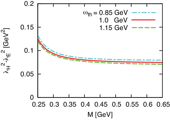
In Figs. 3 and 4, we plot $\lambda_{H}^{2}(\mu)$ and $\lambda_{H}^{2}(\mu)-\lambda_{E}^{2}(\mu)$ at $\mu=1$ GeV as functions of $M$, obtained by taking the ratios of Eqs.(75) and (76), respectively, with Eq.(54). One finds that the values of $\lambda_{H}^{2}$ are larger than those of the splitting $\lambda_{H}^{2}-\lambda_{E}^{2}$, and, in particular, that the curves for the former show sizeable dependence on the parameter $M$. Indeed, this considerable variation of $\lambda_{H}^{2}$ for $0.3~{\rm GeV}\lesssim M\lesssim 0.5~{\rm GeV}$, which was taken in [9] as the “stability window” for the sum rule (54), is responsible for the large errors in Eq.(6). Such poor stability is known to be a common feature to the sum rules for matrix elements of operators with high dimension [12], because the corresponding sum rules are dominated at small $M$ by the condensates of high dimension. For the present case with the dimension-5 operators in Eqs. (4), (5), the behavior of the sum rule (75) for $0.3~{\rm GeV}\lesssim M\lesssim 0.5~{\rm GeV}$ is mainly determined by the term with the quark-gluon-mixed condensate $\langle{\overline{q}}gG\cdot\sigma q\rangle$: this is demonstrated in Fig.5, which shows the separate contributions from each term in the RHS of (75), organized according to the dimension of the associated local operators. On the other hand, the term with $\langle{\overline{q}}gG\cdot\sigma q\rangle$ is absent from the sum rule (76): this sum rule yields a rather stable behavior for $\lambda_{H}^{2}-\lambda_{E}^{2}$ as shown in Fig.4, but the separate contributions of each term in the RHS of Eq.(76), shown in Fig.6, indicate that the nonperturbative corrections do not decrease for increasing dimension $d=0,3$, and $4$ of the associated operators, similarly as in Fig.5. These characteristic behaviors in Figs. 3 and 4 are in contrast to the case of the decay constant, for which the separate contributions to the sum rule (54) are plotted in Fig.7 with the value $\bar{\Lambda}=0.55$ GeV [9]. These results suggest good convergence of the OPE (28) for $X=F$, with the operators of dimension $d\leq 5$, while the convergence of Eq.(28) for $X=3H$, $3S$, at the same level of accuracy, is questionable. Therefore, we will calculate the nonperturbative corrections to Eq.(28), associated with the dimension-6 operators, and evaluate the corresponding modifications to the sum rules (75) and (76), as well as to Eq. (54), in the next section.

The results for the relevant Wilson coefficients, Eqs. (70) and (74), show that only $C_{\sigma}^{3H}$, associated with the dimension-5 quark-gluon-mixed condensate, is of $O(\alpha_{s}^{0})$, while all the other coefficients are of $O(\alpha_{s})$. This is again in contrast to the case of the decay constant, for which all the nonzero coefficients in Eq.(52) are of $O(\alpha_{s}^{0})$. Combined with the behaviors in Figs. 5-7 discussed above, in particular, with those indicating the dominance of the term associated with the dimension-5 operator in Eq.(75), it is desirable to calculate the $O(\alpha_{s})$ correction to this term induced by the next-to-leading order (NLO) correction to the Wilson coefficient $C_{\sigma}^{3H}$ of Eq.(70). It should be also clarified whether $C_{\sigma}^{3S}$ of Eq.(74) receive the $O(\alpha_{s})$ effects. These new $O(\alpha_{s})$ contributions may give the effects comparable with the other $O(\alpha_{s})$ contributions displayed in Figs. 5, 6. We will work out the one-loop matching to calculate the corresponding Wilson coefficients at $O(\alpha_{s})$ in Sec. IV, and derive the modifications to the sum rules for $\lambda_{E,H}^{2}$.

At the leading accuracy in $\alpha_{s}$, all the relevant power corrections to Eq.(28) with $X=F$ are generated from the second term in Eq.(II), and the leading contribution in the ellipses in the middle line of Eq.(48) reads

which determines the power correction associated with the dimension-6 operator. We exploit the following exact relation between matrix elements of the local operators ($\Gamma$ is arbitrary gamma matrix) [23],

which can be derived straightforwardly using the equations of motion, ${\vtop{\halign{#\cr\hfil/\hfil\crcr$D$\crcr}}}q=0$, $D^{\nu}G_{\mu\nu}^{a}=g\sum_{q^{\prime}}\overline{q}^{\prime}\gamma_{\mu}T^{a}q^{\prime}$, where the summation $\sum_{q^{\prime}}$ is over all quark flavors. Thus, Eq.(77) yields

which implies the new power-correction term in the RHS of Eq. (28) with $X=F$, given as [20, 21]

References

- [1] M. Antonelli et al., Phys. Rept. 494, 197 (2010).
- [2] M. Neubert, Phys. Rept. 245, 259 (1994).
- [3] E. Gamiz, C. T. H. Davies, G. P. Lepage, J. Shigemitsu and M. Wingate [HPQCD Collaboration], Phys. Rev. D80, 014503 (2009).
- [4] C. Bernard et al., PoS LATTICE2008, 278 (2008); A. Bazavov et al. [Fermilab Lattice and MILC Collaborations], Phys. Rev. D85, 114506 (2012).
- [5] B. Blossier et al. [ETM Collaboration], JHEP 1004, 049 (2010).
- [6] A. J. Schwartz, AIP Conf. Proc. 1182, 299 (2009).
- [7] K. Ikado et al. [Belle Collaboration], Phys. Rev. Lett. 97, 251802 (2006); K. Hara et al. [Belle Collaboration], Phys. Rev. D82, 071101 (2010); I. Adachi et al. [Belle Collaboration], Phys. Rev. Lett. 110, 131801 (2013).
- [8] B. Aubert et al. [BABAR Collaboration], Phys. Rev. D76, 052002 (2007); P. del Amo Sanchez et al. [BaBar Collaboration], arXiv:1008.0104 [hep-ex]; B. Aubert et al. [BaBar Collaboration], Phys. Rev. D 81, 051101 (2010).
- [9] A. G. Grozin and M. Neubert, Phys. Rev. D55, 272 (1997).
- [10] E. Bagan, P. Ball, V. M. Braun and H. G. Dosch, Phys. Lett. B278, 457 (1992).
- [11] A. A. Penin and M. Steinhauser, Phys. Rev. D65, 054006 (2002).
- [12] A. R. Zhitnitsky, I. R. Zhitnitsky and V. L. Chernyak, Sov. J. Nucl. Phys. 41, 284 (1985) [Yad. Fiz. 41, 445 (1985)]; V. M. Braun and I. E. Filyanov, Z. Phys. C48, 239 (1990); P. Ball, V. M. Braun, Y. Koike and K. Tanaka, Nucl. Phys. B529, 323 (1998).
- [13] H. Kawamura, J. Kodaira, C.F. Qiao and K. Tanaka, Phys. Lett. B523, 111 (2001); Erratum-ibid. B536, 344 (2002); Mod. Phys. Lett. A18, 799 (2003); Nucl. Phys. B (Proc. Suppl.) 116, 269 (2003); H. Kawamura, J. Kodaira and K. Tanaka, Prog. Theor. Phys. 113, 183 (2005).
- [14] T. Huang, X. G. Wu and M. Z. Zhou, Phys. Lett. B611, 260 (2005); B. Geyer and O. Witzel, Phys. Rev. D72, 034023 (2005); T. Huang, C. F. Qiao and X. G. Wu, Phys. Rev. D73, 074004 (2006); B. Geyer and O. Witzel, Phys. Rev. D76, 074022 (2007); A. Khodjamirian, T. Mannel and N. Offen, Phys. Lett. B620, 52 (2005); A. Khodjamirian, T. Mannel and N. Offen, Phys. Rev. D75, 054013 (2007); A. Le Yaouanc, L. Oliver and J. C. Raynal, Phys. Rev. D77, 034005 (2008).
- [15] V. M. Braun, D. Y. Ivanov and G. P. Korchemsky, Phys. Rev. D69, 034014 (2004).
- [16] S. J. Lee and M. Neubert, Phys. Rev. D72, 094028 (2005).
- [17] S. Descotes-Genon and N. Offen, JHEP 0905, 091 (2009); M. Knodlseder and N. Offen, JHEP 1110, 069 (2011).
- [18] H. Kawamura and K. Tanaka, Phys. Lett. B673, 201 (2009); H. Kawamura and K. Tanaka, Phys. Rev. D81, 114009 (2010).
- [19] G. Bell and V. Pilipp, Phys. Rev. D80, 054024 (2009); M. Beneke, T. Huber and X. Q. Li, Nucl. Phys. B832, 109 (2010).
- [20] E. V. Shuryak, Nucl. Phys. B198, 83 (1982).
- [21] M. Neubert, Phys. Rev. D45, 2451 (1992).
- [22] V. A. Novikov, M. A. Shifman, A. I. Vainshtein and V. I. Zakharov, Fortsch. Phys. 32, 585 (1984).
- [23] See, e.g., A. G. Grozin, Int. J. Mod. Phys. A10, 3497 (1995).
- [24] L. F. Abbott, Nucl. Phys. B185, 189 (1981); Acta Phys. Polon. B13, 33 (1982).
- [25] S. Narison and R. Tarrach, Phys. Lett. B125, 217 (1983).
- [26] A. Y. Morozov, Sov. J. Nucl. Phys. 40, 505 (1984); Preprints ITEP-190, 191 (1983).
- [27] X. -D. Ji and M. J. Musolf, Phys. Lett. B257, 409 (1991); D. J. Broadhurst and A. G. Grozin, Phys. Lett. B267, 105 (1991).
- [28] D. J. Broadhurst and A. G. Grozin, Phys. Lett. B274, 421 (1992).
- [29] S. Narison, Camb. Monogr. Part. Phys. Nucl. Phys. Cosmol. 17, 1 (2002).
- [30] P. Ball and V. M. Braun, Phys. Rev. D 49, 2472 (1994) [hep-ph/9307291].
- [31] M. Neubert, Phys. Rev. D46, 1076 (1992).
- [32] K. Nakamura et al. [Particle Data Group], J. Phys. G 37, 075021 (2010).
- [33] H. D. Politzer, Nucl. Phys. B172, 349 (1980); J. C. Collins, Renormalization, (Cambridge University Press, 1984); J. Kodaira and K. Tanaka, Prog. Theor. Phys. 101, 191 (1999).
- [34] J. Kodaira, Y. Yasui and T. Uematsu, Phys. Lett. B344, 348 (1995); J. Kodaira, Y. Yasui, K. Tanaka and T. Uematsu, Phys. Lett. B387, 855 (1996); Y. Koike and K. Tanaka, Phys. Rev. D51, 6125 (1995); Y. Koike and N. Nishiyama, Phys. Rev. D55, 3068 (1997); H. Kawamura, T. Uematsu, J. Kodaira and Y. Yasui, Mod. Phys. Lett. A12, 135 (1997); H. Kawamura, Z. Phys. C75, 27 (1997).
- [35] E. V. Shuryak and A. I. Vainshtein, Nucl. Phys. B199, 451 (1982); B201, 141 (1982); A. P. Bukhvostov, E. A. Kuraev and L. N. Lipatov, Sov. Phys. JETP 60, 22 (1984); I. I. Balitsky and V. M. Braun, Nucl. Phys. B311, 541 (1989); J. Kodaira, T. Nasuno, H. Tochimura, K. Tanaka and Y. Yasui, Prog. Theor. Phys. 99, 315 (1998).
- [36] A. G. Grozin and M. Neubert, Nucl. Phys. B495, 81 (1997).
- [37] P. Ball, V. M. Braun and A. Lenz, JHEP 0605, 004 (2006).