On the relation between Differential Privacy and Quantitative Information Flow Thanks: This work has been partially supported by the project ANR-09-BLAN-0169-01 PANDA and by the INRIA DRI Equipe Associée PRINTEMPS. The work of Miguel E. Andrés has been supported by the LIX-Qualcomm postdoc fellowship 2010.
Abstract
Differential privacy is a notion that has emerged in the community of statistical databases, as a response to the problem of protecting the privacy of the database’s participants when performing statistical queries. The idea is that a randomized query satisfies differential privacy if the likelihood of obtaining a certain answer for a database is not too different from the likelihood of obtaining the same answer on adjacent databases, i.e. databases which differ from for only one individual.
Information flow is an area of Security concerned with the problem of controlling the leakage of confidential information in programs and protocols. Nowadays, one of the most established approaches to quantify and to reason about leakage is based on the Rényi min entropy version of information theory.
In this paper, we analyze critically the notion of differential privacy in light of the conceptual framework provided by the Rényi min information theory. We show that there is a close relation between differential privacy and leakage, due to the graph symmetries induced by the adjacency relation. Furthermore, we consider the utility of the randomized answer, which measures its expected degree of accuracy. We focus on certain kinds of utility functions called “binary”, which have a close correspondence with the Rényi min mutual information. Again, it turns out that there can be a tight correspondence between differential privacy and utility, depending on the symmetries induced by the adjacency relation and by the query. Depending on these symmetries we can also build an optimal-utility randomization mechanism while preserving the required level of differential privacy. Our main contribution is a study of the kind of structures that can be induced by the adjacency relation and the query, and how to use them to derive bounds on the leakage and achieve the optimal utility.
1 Introduction
Databases are commonly used for obtaining statistical information about their participants. Simple examples of statistical queries are, for instance, the predominant disease of a certain population, or the average salary. The fact that the answer is publicly available, however, constitutes a threat for the privacy of the individuals.
In order to illustrate the problem, consider a set of individuals whose attribute of interest11 1 In general we could be interested in several attributes simultaneously, and in this case would be a set of tuples. has values in . A particular database is formed by a subset of , where a certain value in is associated to each participant. A query is a function , where is the set of all possible databases, and is the domain of the answers.
For example, let be the set of possible salaries and let represent the query “what is the average salary of the participants in the database”. In principle we would like to consider the global information relative to a database as public, and the individual information about a participant as private. Namely, we would like to be able to obtain without being able to infer the salary of . However, this is not always possible. In particular, if the number of participants in is known (say ), then the removal of from the database would allow to infer ’s salary by querying again the new database , and by applying the formula . Using an analogous reasoning we can argue that not only the removal, but also the addition of an individual is a threat for his privacy.
Another kind of private information we may want to protect is whether an individual is participating or not in a database. In this case, if we know for instance that earns, say Euros/month, and all the other individuals in earn less than Euros/month, then knowing that Euros/month will reveal immediately that is in the database .
A common solution to the above problems is to introduce some output perturbation mechanism based on randomization: instead of the exact answer we report a “noisy” answer. Namely, we use some randomized function which produces values in some domain22 2 The new domain may coincide with , but not necessarily. It depends on how the randomization mechanism is defined. according to some probability distribution that depends on the input . Of course for certain distributions it may still be possible to guess the value of an individual with a high probability of success. The notion of differential privacy, due to Dwork [10, 13, 11, 12], is a proposal to control the risk of violating privacy for both kinds of threats described above (value and participation). The idea is to say that satisfies -differential privacy (for some ) if the ratio between the probabilities that two adjacent databases give the same answer is bound by , where by “adjacent” we mean that the databases differ for only one individual (either for the value of an individual or for the presence/absence of an individual). Often we will abbreviate “-differential privacy” as -d.p.
Obviously, the smaller is , the greater is the privacy protection. In particular, when is close to the output of is nearly independent from the input (all distributions are almost equal). Unfortunately, such is practically useless. The utility, i.e. the capability to retrieve accurate answers from the reported ones, is the other important characteristic of , and it is clear that there is a trade-off between utility and privacy. On the other hand, these two notions are not the complete opposite of each other, because utility concerns the relation between the reported answer and the real answer, while privacy is concerns the relation between the reported answer and the information in the database. This asymmetry makes more interesting the problem of finding a good compromise between the two.
At this point, we would like to remark an intriguing analogy between the area of differential privacy and that of quantitative information flow (QIF), both in the motivations and in the basic conceptual framework. Information flow is concerned with the leakage of secret information through computer systems, and the attribute “quantitative” refers to the fact that we are interested in measuring the amount of leakage, not just its occurrence. One of the most established approaches to QIF is based on information theory: the idea is that a system is seen as a channel in the information-theoretic sense, where the secret is the input and the observables are the output. The entropy of the input represents its vulnerability, i.e. how easy it is for an attacher to guess the secret. We distinguish between the a priori entropy (before the observable) and the a posteriori entropy (given the observable). The difference between the two gives the mutual information and represents, intuitively, the increase in vulnerability due to the observables produced by the system, so it is naturally considered as a measure of the leakage. The notion of entropy is related to the kind of attack we want to model, and in this paper we focus on the Rényi min entropy [18], which represents the so-called one-try attacks. In recent years there has been a lot of research aimed at establishing the foundations of this framework [19, 7, 16, 3, 5]. It is worth pointing out that the a posteriori Rényi min entropy corresponds to the concept of Bayes risk, which has also been proposed as a measure of the effectiveness of attacks [8, 6, 17].
The analogy hinted above between differential privacy and QIF is based on the following observations: at the motivational level, the concern about privacy is akin the concern about information leakage. At the conceptual level, the randomized function can be seen as an information-theoretic channel, and the limit case of , for which the privacy protection is total, corresponds to a -capacity channel33 3 The channel capacity is the maximum mutual information over all possible input distributions. (the rows of the channel matrix are all identical), which does not allow any leakage. Another promising similarity is that the notion of utility (in the binary case) corresponds closely to the Bayes risk.
In this paper we investigate the notion of differential privacy, and its implications, in light of the min-entropy information theoretic framework developed for QIF. In particular, we wish to explore the following natural questions:
- 1.
Does -d.p. induce a bound on the information leakage of ?
- 2.
Does -d.p. induce a bound on the information leakage relative to an individual?
- 3.
Does -d.p. induce a bound on the utility?
- 4.
Given and , can we construct a which satisfies -d.p. and maximum utility?
We will see that the answers to (1) and (2) are positive, and we provide bounds that are tight, in the sense that for every there is a whose leakage reaches the bound. For (3) we are able to give a tight bound in some cases which depend on the structure of the query, and for the same cases, we are able to construct an oblivious44 4 A randomized function is oblivious if its probability distribution depends only on the answer to the query, and not on the database. with maximum utility, as requested by (4).
Part of the above results have already appeared in [1], and are based on techniques which exploit the graph structure that the adjacency relation induces on the domain of all databases , and on the domain of the correct answers . The main contribution of this paper is an extension of those techniques, and a coherent graph-theoretic framework for reasoning about the symmetries of those domains. More specifically:
- •
We explore the graph-theoretic foundations of the adjacency relation, and point out various types of symmetries which allow us to establish a strict link between differential privacy and information leakage.
- •
We give a tight bound for the question (2) above, strictly smaller than the one in [1].
- •
We extend the structures for which we give a positive answer to the questions (3) and (4) above. In [1] the only case considered was the class of graphs with single-orbit automorphisms. Here we show that the results hold also for regular-distance graphs and a variant of vertex-transtive graphs.
In this paper we focus on the case in which , and are finite, leaving the more general case for future work.
2 Preliminaries
2.1 Database domain and Differential privacy
Let be a finite set of individuals that may participate in a database and a finite set of possible values for the attribute of interest of these individuals. In order to capture in a uniform way the presence/absence of an individual in the database, as well as its value, we enrich the set of possible values with an element representing the absence of the individual. Thus the set of all possible databases is the set , where . We will use and to denote the cardinalities of and , and , respectively. Hence we have that . A database can be represented as a -tuple where each is the value of the corresponding individual. Two databases are adjacent (or neighbors), written , if they differ for the value of exactly one individual. For instance, for , and , with , are adjacent. The structure forms an undirected graph.
Intuitively, differential privacy is based on the idea that a randomized query function provides sufficient protection if the ratio between the probabilities of two adjacent databases to give a certain answer is bound by , for some given . Formally:
Definition 1 ([12])
A randomized function from to satisfies -differential privacy if for all pairs , with , and all , we have that:
The above definition takes into account the possibility that is a continuous domain. In our case, since is finite, the probability distribution is discrete, and we can rewrite the property of -d.p. more simply as (using the notation of conditional probabilities, and considering both quotients):
where and represent the random variables associated to and , respectively.
2.2 Information theory and application to information flow
In the following, denote two discrete random variables with carriers , , and probability distributions , , respectively. An information-theoretic channel is constituted by an input , an output , and the matrix of conditional probabilities , where represent the probability that is given that is . We shall omit the subscripts on the probabilities when they are clear from the context.
Rényi min-entropy
In [18], Rényi introduced an one-parameter family of entropy measures, intended as a generalization of Shannon entropy. The Rényi entropy of order (, ) of a random variable is defined as . We are particularly interested in the limit of as approaches . This is called min-entropy. It can be proven that .
Rényi defined also the -generalization of other information-theoretic notions, like the Kullback-Leibler divergence. However, he did not define the -generalization of the conditional entropy, and there is no general agreement on what it should be. For the case , we adopt here the definition of conditional entropy proposed by Smith in [19]:
| (1) |
Analogously to the Shannon case, we can define the Rényi-mutual information as , and the capacity as . It has been proven in [7] that is obtained at the uniform distribution, and that it is equal to the sum of the maxima of each column in the channel matrix, i.e., .
Interpretation in terms of attacks:
Rényi min-entropy can be related to a model of adversary who is allowed to ask exactly one question, which must be of the form “is ” (one-try attacks). More precisely, represents the (logarithm of the inverse of the) probability of success for this kind of attacks and with the best strategy, which consists, of course, in choosing the with the maximum probability.
As for , it represents the inverse of the (expected value of the) probability that the same kind of adversary succeeds in guessing the value of a posteriori, i.e. after observing the result of . The complement of this probability is also known as Bayes risk. Since in general and are correlated, observing increases the probability of success. Indeed we can prove formally that , with equality if and only if and are independent. corresponds to the ratio between the probabilities of success a priori and a posteriori, which is a natural notion of leakage. Note that , which seems desirable for a good notion of leakage.
3 Graph symmetries
In this section we explore some classes of graphs that allow us to derive a strict correspondence between -d.p. and the a posteriori entropy of the input.
Let us first recall some basic notions. Given a graph , the distance between two vertices is the number of edges in a shortest path connecting them. The diameter of is the maximum distance between any two vertices in . The degree of a vertex is the number of edges incident to it. is called regular if every vertex has the same degree. A regular graph with vertices of degree is called a -regular graph. An automorphism of is a permutation of the vertex set , such that for any pair of vertices , if , then . If is an automorphism, and a vertex, the orbit of under is the set where is the smallest positive integer such that . Clearly, the orbits of the vertices under define a partition of .
The following two definition introduce the classes of graphs that we are interested in. The first class is well known in literature.
Definition 2
Given a graph , we say that is distance-regular if there exist integers such that for any two vertices in with distance , there are exactly neighbors of in and neighbors of in , where is the set of vertices of with .
Some examples of distance-regular graphs are illustrated in Figure 1.


The next class is a variant of the VT (vertex-transitive) class:
Definition 3
A graph is VT+ (vertex-transitive +) if there are automorphisms , , …, where , such that, for every vertex , we have that .
In particular, the graphs for which there exists an automorphism which induces only one orbit are VT+: in fact it is sufficient to define for all from to . Figure 2 illustrates some graphs with a single-orbit automorphism.


From graph theory we know that neither of the two classes subsumes the other. They have however a non-empty intersection, which contains in particular all the structures of the form , i.e. the database domains.
Proposition 1
The structure is both a distance-regular graph and a VT+ graph.
Figure 3 illustrates some examples of structures . Note that when and , is the -dimentional hypercube.
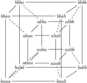

The situation is summarized in Figure 4. We remark that in general the graphs do not have a single-orbit automorphism. The only exceptions are the two simplest structures ().

The two symmetry classes defined above, distance-regular and VT+, will be used in the next section to transform a generic channel matrix into a matrix with a symmetric structure, while preserving the a posteriori min entropy and the -d.p.. This is the core of our technique to establish the relation between differential privacy and quantitive information flow, depending on the structure induced by the database adjacency relation.
4 Deriving the relation between differential privacy and QIF on the basis of the graph structure
This section contains the main technical contribution of the paper: a general technique for determining the relation between -differential privacy and leakage, and between -differential privacy and utility, depending on the graph structure induced by and . The idea is to use the symmetries of the graph structure to transform the channel matrix into an equivalent matrix with certain regularities, which allow to establish the link between -differential privacy and the a posteriori min entropy.
Let us illustrate briefly this transformation. Consider a channel whose matrix has at least as many columns as rows. First, we transform into a matrix in which each of the first columns has a maximum in the diagonal, and the remaining columns are all ’s. Second, under the assumption that the input domain is distance-regular or VT+, we transform into a matrix whose diagonal elements are all the same, and coincide with the maximum element of , which we denote here by . These steps are illustrated in Figure 5.
We are now going to present formally our the technique. Let us first fix some notation: In the rest of this section we consider channels with input and output , with carriers and respectively, and we assume that the probability distribution of is uniform. Furthermore, we assume that . We also assume an adjacency relation on , i.e. that is an undirected graph structure. With a slight abuse of notation, we will also write when and are associated to adjacent elements of , and we will write to denote the distance between the elements of associated to and .
We note that a channel matrix satisfies -d.p. if for each column and for each pair of rows and such that we have that:
The a posteriori entropy of a channel with matrix will be denoted by .

Next Lemma is relative to the first step of the transformation.
Lemma 1
Consider a channel with matrix . Assume that satisfies -d.p.. Then it is possible to transform into a matrix such that:
- •
Each of the first columns has a maximum in the diagonal, i.e. for each from to .
- •
The rest of the columns contain only ’s, i.e. for each from to and each from to .
- •
satisfies -d.p.
- •
.
Next lemma is relative to the second step of the transformation, for the case of distance-regular graphs.
Lemma 2
Consider a channel with matrix . Assume that satisfies -d.p., and the first columns have maxima in the diagonal, and the rest of the columns contain only ’s. Assume that is distance-regular. Then it is possible to transform into a matrix such that:
- •
The elements of the diagonal are all the same, and are equal to the maximum of the matrix, i.e. for each from to .
- •
The rest of the columns contain only ’s.
- •
satisfies -d.p.
- •
.
Next lemma is relative to the second step of the transformation, for the case of VT+ graphs.
Lemma 3
Note that the fact that in the diagonal elements are all equal to the maximum implies that .
Once we have a matrix with the properties of , we can use again the graph structure of to determine a bound on .
First we note that the property of -d.p. induces a relation between the ratio of elements at any distance:
Remark 1
Let be a matrix satisfying -d.p.. Then, for any column , and any pair of rows and we have that:
In particular, if we know that the diagonal elements of are equal to the maximum element , then for each element we have that:
| (2) |
Let us fix a row, say row . For each distance from to the diameter of the graph, let be the number of elements that are at distance from the corresponding diagonal element , i.e. such that . (Clearly, depends on the structure of the graph.) Since the elements of the row represent a probability distribution, we obtain the following dis-equation:
from which we derive immediately a bound on the min a-posteriori entropy.
Putting together all the steps of this section, we obtain our main result.
Theorem 4.1
Consider a matrix , and let be a row of . Assume that is either distance-regular or VT+, and that satisfies -d.p. For each distance from to the diameter of , let be the number of nodes at distance from . Then we have that:
| (3) |
Note that this bound is tight, in the sense that we can build a matrix for which (3) holds with equality. It is sufficient to define each element according to (2) (with equality instead of dis-equality, of course).
In the next section, we will see how to use this theorem for establishing a bound on the leakage and on the utility.
5 Application to leakage
As already hinted in the introduction, we can regard as a channel with input and output . From Proposition 1 we know that is both distance-regular and VT+, we can therefore apply Theorem 4.1. Let us fix a particular database . The number of databases at distance from is
| (4) |
where and . In fact, recall that can be represented as a -tuple with values in . We need to select individuals in the -tuple and then change their values, and each of them can be changed in different ways.
Using the from (4) in Theorem 4.1 we obtain a binomial expansion in the denominator, namely:
which gives the following result:
Theorem 5.1
If satisfies -d.p., then for the uniform input distribution the information leakage is bound from above as follows:
We consider now the leakage for a single individual. Let us fix a database , and a particular individual in . The possible ways in which we can change the value of in are . All the new databases obtained in this way are adjacent to each other, i.e. the graph structure associated to the input is a clique of nodes. Therefore we obtain for , for , and otherwise. By substituting this value of in Theorem 4.1, we get
which leads to the following result:
Proposition 2
Assume that satisfies -d.p.. Then for the uniform distribution on the information leakage for an individual is bound from above as follows:
Note that the bound on the leakage for an individual does not depend on the size of , nor on the database that we fix.
6 Application to utility
We turn now our attention to the issue of utility. We focus on the case in which is oblivious, which means that it depends only on the (exact) answer to the query, i.e. on the value of , and not on .
An oblivious function can be decomposed in the concatenation of two channels, one representing the function , and the other representing the randomization mechanism added as output perturbation. The situation is illustrated in Figure 6.

The standard way to define utility is by means of and functions. The functionality of the first is , and it represents the user’s strategy to retrieve the correct answer form the reported one. The functionality of the latter is . the value represents the reward for guessing the answer when the correct answer is . The utility can then be defined as the expected gain:
We focus here on the so-called binary gain function, which is defined as
This kind of function represents the case in which there is no reason to prefer an answer over the other, except if it is the right answer. More precisely, we get a gain if and only if we guess the right answer.
If the gain function is binary, and the function represents the user’s best strategy, i.e. it is chosen to optimize utility, then there is a well-known correspondence between and the Bayes risk / the a posteriori min entropy. Such correspondence is expressed by the following proposition:
Proposition 3
Assume that is binary and is optimal. Then:
In order to analyze the implications of the -d.p. requirement on the utility, we need to consider the structure that the adjacency relation induces on . Let us define on as follows: if there are such that , , and . Note that satisfies -d.p. if and only if satisfies -d.p.
If is distance-regular or VT+, then we can apply Theorem 4.1 to find a bound on the utility. In the following, we assume that the distribution of is uniform.
Theorem 6.1
Consider a randomized mechanism , and let be an element of . Assume that is either distance-regular or VT+ and that satisfies -d.p. For each distance from to the diameter of , let be the number of nodes at distance from . Then we have that:
| (5) |
The above bound is tight, in the sense that (provided is distance-regular or VT+) we can construct a mechanism which satisfies (5) with equality. More precisely, define
Then define (here identified with its channel matrix for simplicity) as follows:
| (6) |
Theorem 6.2
Assume is distance-regular or VT+. Then the matrix defined in (6) satisfies -d.p. and has maximal utility:
Note that we can always define as in (6): the matrix so defined will be a legal channel matrix, and it will satisfy -d.p.. However, if is neither distance-regular nor VT+, then the utility of such is not necessarily optimal.
We end this section with an example (borrowed from [1]) to illustrate our technique.
Example 1
Consider a database with electoral information where each row corresponds to a voter and contains the following three fields:
- •
Id: a unique (anonymized) identifier assigned to each voter;
- •
City: the name of the city where the user voted;
- •
Candidate: the name of the candidate the user voted for.
Consider the query “What is the city with the greatest number of votes for a given candidate ?”. For such a query the binary utility function is the natural choice: only the right city gives some gain, and all wrong answers are equally bad. It is easy to see that every two answers are neighbors, i.e. the graph structure of the answers is a clique.
Let us consider the scenario where City and assume for simplicity that there is a unique answer for the query, i.e., there are no two cities with exactly the same number of individuals voting for candidate . Table 1 shows two alternative mechanisms providing -differential privacy (with ). The first one, , is based on the truncated geometric mechanism method used in [14] for counting queries (here extended to the case where every pair of answers is neighbor). The second mechanism, , is obtained by applying the definition (6). From Theorem 6.2 we know that for the uniform input distribution gives optimal utility.
For the uniform input distribution, it is easy to see that . Even for non-uniform distributions, our mechanism still provides better utility. For instance, for and , we have . This is not too surprising: the geometric mechanism, as well as the Laplacian mechanism proposed by Dwork, perform very well when the domain of answers is provided with a metric and the utility function is not binary55 5 In the metric case the gain function can take into account the proximity of the reported answer to the real one, the idea being that a close answer, even if wrong, is better than a distant one.. It also works well when has low connectivity, in particular in the cases of a ring and of a line. But in this example, we are not in these cases, because we are considering binary gain functions and high connectivity.
7 Related work
As far as we know, the first work to investigate the relation between differential privacy and information-theoretic leakage for an individual was [2]. In this work, a channel is relative to a given database , and the channel inputs are all possible databases adjacent to . Two bounds on leakage were presented, one for teh Rényi min entropy, and one for Shannon entropy. Our bound in Proposition 2 is an improvement with respect to the (Rényi min entropy) bound in [2].
Barthe and Köpf [4] were the first to investigates the (more challenging) connection between differential privacy and the Rényi min-entropy leakage for the entire universe of possible databases. They consider the “end-to-end differentially private mechanisms”, which correspond to what we call in our paper, and propose, like we do, to interpret them as information-theoretic channels. They provide a bound for the leakage, but point out that it is not tight in general, and show that there cannot be a domain-independent bound, by proving that for any number of individual the optimal bound must be at least a certain expression . Finally, they show that the question of providing optimal upper bounds for the leakage of -differentially private randomized functions in terms of rational functions of is decidable, and leave the actual function as an open question. In our work we used rather different techniques and found (independently) the same function (the bound in Theorem 4.1), but we actually proved that is the optimal bound66 6 When discussing our result with Barthe and Köpf, they said that they also conjectured that is the optimal bound.. Another difference is that [4] captures the case in which the focus of differential privacy is on hiding participation of individuals in a database. In our work, we consider both the participation and the values of the participants.
Clarkson and Schneider also considered differential privacy as a case study of their proposal for quantification of integrity [9]. There, the authors analyze database privacy conditions from the literature (such as differential privacy, -anonymity, and -diversity) using their framework for utility quantification. In particular, they study the relationship between differential privacy and a notion of leakage (which is different from ours - in particular their definition is based on Shannon entropy) and they provide a tight bound on leakage.
Heusser and Malacaria [15] were among the first to explore the application of information-theoretic concepts to databases queries. They proposed to model database queries as programs, which allows for statical analysis of the information leaked by the query. However [15] did not attempt to relate information leakage to differential privacy.
In [14] the authors aim at obtaining optimal-utility randomization mechanisms while preserving differential privacy. The authors propose adding noise to the output of the query according to the geometric mechanism. Their framework is very interesting in the sense it provides a general definition of utility for a mechanism that captures any possible side information and preference (defined as a loss function) the users of may have. They prove that the geometric mechanism is optimal in the particular case of counting queries. Our results in Section 6 do not restrict to counting queries, but on the other hand we only consider the case of binary loss function.
8 Conclusion and future work
In this paper we have investigated the relation between -differential privacy and leakage, and between -differential privacy and utility. Our main contribution is the development of a general technique for determining these relations depending on the graph structure induced by the adjacency relation and by the query. We have considered two particular structures, the distance-regular graphs, and the VT+ graphs, which allow to obtain tight bounds on the leakage and on the utility, and to construct the optimal randomization mechanism satisfying -differential privacy.
As future work, we plan to extend our result to other kinds of utility functions. In particular, we are interested in the case in which the the answer domain is provided with a metric, and we are interested in taking into account the degree of accuracy of the inferred answer.
References
- [1] Mário S. Alvim, Miguel E. Andrés, Konstantinos Chatzikokolakis, Pierpaolo Degano, and Catuscia Palamidessi. Differential privacy: on the trade-off between utility and information leakage. Technical report, 2011. http://hal.inria.fr/inria-00580122/en/.
- [2] Mário S. Alvim, Konstantinos Chatzikokolakis, Pierpaolo Degano, and Catuscia Palamidessi. Differential privacy versus quantitative information flow. Technical report, 2010.
- [3] Miguel E. Andrés, Catuscia Palamidessi, Peter van Rossum, and Geoffrey Smith. Computing the leakage of information-hiding systems. In Proc. of TACAS, volume 6015 of LNCS, pages 373–389. Springer, 2010.
- [4] Gilles Barthe and Boris Köpf. Information-theoretic bounds for differentially private mechanisms. In Proc. of CSF, 2011. To appear.
- [5] Michele Boreale, Francesca Pampaloni, and Michela Paolini. Asymptotic information leakage under one-try attacks. In Proc. of FOSSACS, volume 6604 of LNCS, pages 396–410. Springer, 2011.
- [6] Christelle Braun, Konstantinos Chatzikokolakis, and Catuscia Palamidessi. Compositional methods for information-hiding. In Proc. of FOSSACS, volume 4962 of LNCS, pages 443–457. Springer, 2008.
- [7] Christelle Braun, Konstantinos Chatzikokolakis, and Catuscia Palamidessi. Quantitative notions of leakage for one-try attacks. In Proc. of MFPS, volume 249 of ENTCS, pages 75–91. Elsevier, 2009.
- [8] Konstantinos Chatzikokolakis, Catuscia Palamidessi, and Prakash Panangaden. Probability of error in information-hiding protocols. In Proc. of CSF, pages 341–354. IEEE, 2007.
- [9] M. R. Clarkson and F. B. Schneider. Quantification of integrity, 2011. Tech. Rep.. http://hdl.handle.net/1813/22012.
- [10] Cynthia Dwork. Differential privacy. In Automata, Languages and Programming, 33rd Int. Colloquium, ICALP 2006, Venice, Italy, July 10-14, 2006, Proc., Part II, volume 4052 of LNCS, pages 1–12. Springer, 2006.
- [11] Cynthia Dwork. Differential privacy in new settings. In Proc. of the Twenty-First Annual ACM-SIAM Symposium on Discrete Algorithms, SODA 2010, Austin, Texas, USA, January 17-19, 2010, pages 174–183. SIAM, 2010.
- [12] Cynthia Dwork. A firm foundation for private data analysis. Communications of the ACM, 54(1):86–96, 2011.
- [13] Cynthia Dwork and Jing Lei. Differential privacy and robust statistics. In Proc. of the 41st Annual ACM Symposium on Theory of Computing, STOC 2009, Bethesda, MD, USA, May 31 - June 2, 2009, pages 371–380. ACM, 2009.
- [14] Arpita Ghosh, Tim Roughgarden, and Mukund Sundararajan. Universally utility-maximizing privacy mechanisms. In Proc. of the 41st annual ACM symposium on Theory of computing, STOC ’09, pages 351–360. ACM, 2009.
- [15] Jonathan Heusser and Pasquale Malacaria. Applied quantitative information flow and statistical databases. In Proc. of the Int. Workshop on Formal Aspects in Security and Trust, volume 5983 of LNCS, pages 96–110. Springer, 2009.
- [16] Boris Köpf and Geoffrey Smith. Vulnerability bounds and leakage resilience of blinded cryptography under timing attacks. In Proc. of CSF, pages 44–56. IEEE, 2010.
- [17] Annabelle McIver, Larissa Meinicke, and Carroll Morgan. Compositional closure for bayes risk in probabilistic noninterference. In Proc. of ICALP, volume 6199 of LNCS, pages 223–235. Springer, 2010.
- [18] Alfréd Rényi. On Measures of Entropy and Information. In Proc. of the 4th Berkeley Symposium on Mathematics, Statistics, and Probability, pages 547–561, 1961.
- [19] Geoffrey Smith. On the foundations of quantitative information flow. In Proc. of FOSSACS, volume 5504 of LNCS, pages 288–302. Springer, 2009.