Electromagnetic Excitation of Nucleon Resonances

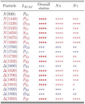
Our knowledge about the excitation spectrum of the nucleon was originally provided by elastic pion-nucleon scattering. All the resonances listed in the Particle Data Tables (PDG) [1] were identified by partial-wave analyses of this process with both Breit-Wigner and pole extraction techniques. In PDG the nucleon resonances $N^{*}$ and $\Delta$ are given a status from one-star for a ‘poor evidence of existing’ up to four-star for a ‘certain existence’, where ‘properties are at least fairly well explored’. In Fig. 1 we show part of the PDG summary table including only three- and four-star resonances up to a mass of 2 GeV. But out of 13 four-star resonances, only 5 are listed with also four stars in the $N\gamma$ channel. For others the e.m. properties are at best only approximately known. From partial wave analyses we know the resonance masses, widths, pole positions, and branching ratios into the $\pi N$ and $\pi\pi N$ channels. These are reliable parameters for the four-star resonances, with only few exceptions. In particular, there remains some doubt about the structure of two prominent resonances, the Roper $P_{11}(1440)$, which appears unusually broad, and the $S_{11}(1535)$ whose pole position can not be uniquely determined because its closeness to the $\eta N$ threshold. In Figs. 2-3 we have mapped the $P_{33}$ and $P_{11}$ partial waves in the complex energy plane, as derived from an analysis within the Dubna-Mainz-Taipei dynamical meson-exchange model [2, 3]. In both cases, the plots show 3-4 poles for imaginary values of $W$ from zero down to about $-250$ MeV. The residues of the poles are proportional to the size of the white disks in the figures. However, one should keep in mind that the influence of a pole on the physical region decreases rapidly with the distance from the real axis.

On the basis of these relatively firm grounds, additional information can be obtained for the electromagnetic (e.m.) $\gamma NN^{*}$ couplings through meson photo- and electroproduction. By far, the main source for resonance structure is pion production, but in some cases with a small $\pi N$ branching ratio, also $\eta$, $\pi\pi$, $K$, $\rho$, $\omega$, etc. production can give valuable information. A typical such example is the $S_{11}(1535)$ resonance, which is located close to the $\eta N$ threshold and strongly coupled to this channel.

Here we will concentrate on the analysis of pion photo- and electroproduction. The $\gamma N$ couplings can be given in terms of electric, magnetic, and Coulomb transition moments or, alternatively, as helicity amplitudes. The PDG lists only the helicity amplitudes $A_{1/2}$ and $A_{3/2}$ for real photons. These amplitudes are real numbers, which are determined at the Breit-Wigner position of a given resonance. In electroproduction, an additional longitudinal amplitude $S_{1/2}(Q^{2})$ can be determined and all three amplitudes become functions of $Q^{2}$. In particular for the $N\to\Delta$ transition, a set of 3 Sachs form factors ($G_{E}^{*}$, $G_{M}^{*}$, $G_{C}^{*}$) is often introduced and, most recently, also a set of covariant Dirac form factors ($F_{1}^{NN^{*}},F_{2}^{NN^{*}}$, $F_{3}^{NN^{*}}$) has been used, especially for comparison with lattice QCD and as a source to derive transverse transition densities in the light-front frame. A general derivation of $NN^{*}$ transition form factors for arbitrary spin and parity states can be found in the paper by Devenish, Eisenschitz, and Körner [4].

Until about 10 years ago, information on the transition form factors (FF) at finite $Q^{2}$ was very scarce and, in particular, nonexistent for the longitudinal form factor. The best knowledge we had was on the magnetic $N\to\Delta(1232)$ form factor $G_{M}^{*}(Q^{2})$, which was fairly well known up to about $Q^{2}=10~{\rm{GeV}}^{2}$. This is the only $NN^{*}$ transition form factor which can be directly measured in inclusive electron scattering [5, 6, 7, 8, 9, 10, 11, 12] because of the very strong $M1$ transition to the isolated $\Delta(1232)$ resonance.

The new era started with $\pi^{0}$ electroproduction experiments at Mainz [13, 14, 15], Bonn [16, 17], and Bates [18, 19] in search for the small $E2$ and $C2$ transition form factors for $N\to\Delta$ and the determination of the $E/M$ and $S/M$ ratios.

Already in the mid-nineties, the resonant multipoles (FFs at $Q^{2}=0$) and in particular the $E/M$ ratio were investigated in experimental programs at MAMI in Mainz [20] and LEGS in Brookhaven [21]. In Fig. 4 we display the $P_{33}$ amplitudes as derived from unpolarized differential cross sections and photon beam asymmetries measured with MAMI B for both $p(\gamma,\pi^{0})p$ and $p(\gamma,\pi^{+})n$. The shown results are based on a model-independent partial wave analysis as performed by the Mainz group during the years 1995-2000. With the well justified assumptions of the Watson theorem (due to unitarity) and the neglect of non-Born D and higher wave contributions, the measurement of only 2 observables for each channel was sufficient to determine the partial waves without any model input. From the $E_{1+}^{3/2}$ and $M_{1+}^{3/2}$ multipoles, the following $\Delta(1232)$ resonance properties were obtained [20, 24, 22, 23]:

• •

  e.m. transition moments and $R_{EM}$ ratio at $W_{\rm{res}}=1232$ MeV

  	$\displaystyle\mu_{N\Delta}$	$\displaystyle=$	$\displaystyle\quad(3.46\pm 0.03)\,\mu_{N}\,,$		(1)
  	$\displaystyle Q_{N\Delta}$	$\displaystyle=$	$\displaystyle-(0.0846\pm 0.0033)\,\mbox{fm}^{2}\,,$		(2)
  	$\displaystyle R_{EM}$	$\displaystyle=$	$\displaystyle-(2.5\pm 0.1_{stat.}\pm 0.2_{syst.})\,\%$		(3)

• •

  pole position and residues at $W_{\rm{pole}}=M_{p}-i/2\,\Gamma_{p}$

  	$\displaystyle M_{p}$	$\displaystyle=$	$\displaystyle(1212\pm 1)\,\mbox{MeV}\,,$		(4)
  	$\displaystyle\Gamma_{p}$	$\displaystyle=$	$\displaystyle(99\pm 2)\,\mbox{MeV}\,,$		(5)
  	$\displaystyle r(M1)$	$\displaystyle=$	$\displaystyle 21.16\cdot e^{-i\,27.5^{\circ}}\,10^{-3}/m_{\pi}\,,$		(6)
  	$\displaystyle r(E2)$	$\displaystyle=$	$\displaystyle 1.23\cdot e^{-i\,154.7^{\circ}}\,10^{-3}/m_{\pi}\,,$		(7)
  	$\displaystyle R_{\Delta}=\frac{r(E2)}{r(M1)}$	$\displaystyle=$	$\displaystyle-0.035-0.046\,i\,.$		(8)

During the last decade, a big step forward was made at JLab [25, 26, 27, 28, 29, 30, 31, 32, 33, 34] by a series of experiments measuring electroproduction of $\pi^{0}$ and $\pi^{+}$ on the proton. Most of these experiments did not use polarization degrees of freedom, except for the longitudinal and transverse polarizations of the virtual photon in electroproduction, which are accessible in experiments with large (azimuthal) angular coverage. However, especially in the $\Delta(1232)$ region, some experiments were performed also with polarized electrons and polarized targets. In Hall A, Kelly et al. [30] even performed an almost complete experiment, which yielded 16 unpolarized and recoil polarization observables at $Q^{2}=1.0$ GeV².

In parallel with the ongoing experiments, several theoretical groups developed models and analysis techniques, which were applied to the data. The model-independent GWU/SAID analysis [35, 36] mostly analyzed the pion photoproduction data and improved the values of the photon couplings over the years. In addition, this group analyzed also the $N\Delta$ transition form factors [37]. However, the model-independent ansatz used in the SAID analysis could not determine the $Q^{2}$ dependence of the transition form factors in a reliable way because of rather limited experimental input from polarization observables. Further coupled channels analyses were performed by the Giessen group [38, 39] and by the Bonn-Gatchina group [40, 41]. Transition amplitudes were also determined in the framework of dynamically generated resonances by coupling to meson-baryon channels, e.g., for the $S_{11}(1535)$ resonance by the Jülich group [42, 43, 44]. In addition, the nature of $N^{*}$ resonances and their physical meaning was investigated within chiral effective field theory [45, 46, 47], and in particular the $\Delta(1232)$ magnetic form factor and the $E/M$ ratio was evaluated by different approaches [48, 49, 50, 51]. Furthermore, dynamical models as the Dubna-Mainz-Taipei (DMT) model [52, 53] and the Sato-Lee model [54] as well as its extensions by the EBAC group [55, 56] were used to analyze photo- and electroproduction in the framework of bare and dressed nucleon resonances. However, most successful concerning the general applicability to the higher resonances, were the unitary isobar models of the Mainz group (MAID model) [57, 58, 59, 60, 61] and of the JLab group [62, 63, 64] who used dispersion relations as an additional constraint to reduce the model dependence due to incomplete experimental input.

With our unitary isobar model MAID, we analyzed all available electroproduction data in order to determine the transition form factors for all four-star resonances below $W=1.8$ GeV. In most cases we could obtain both single-$Q^{2}$ and $Q^{2}$-dependent transition form factors for the proton target. In the case of the neutron, the parametrization of the $Q^{2}$ dependence had to take a simpler form because of the much smaller world database. Already in 2003 [59] we obtained transverse transition form factors for the $\Delta(1232),\,P_{11}(1440),\,S_{11}(1535),\,D_{13}(1520)$, and $F_{15}(1680)$ as well as longitudinal form factors for the $\Delta(1232),\,P_{11}(1440)$, and $S_{11}(1535)$ by using unpolarized $\pi^{0}$ electroproduction data in the range of $Q^{2}=0.4-1.5~GeV^{2}$ [27, 26].

The main motivation for exploring the nucleon transition form factors is to obtain a precise knowledge of the nucleon excitation spectrum, which provides — together with the elastic form factors — a complete description of the nucleon’s electromagnetic structure. This structure can be compared with QCD inspired quark models and, in recent years, more and more also with lattice QCD calculations [65, 66, 67, 68]. Moreover, the nucleon transition form factors provide an essential input for dispersive calculations of both sum rules and two-photon corrections to electron scattering [69, 70, 71, 72, 73].

Finally, the precise e.m. FF data yield the information to map out the quark charge densities in a baryon. A proper interpretation of such densities was found by looking at the baryon in the light-front frame. This procedure yields the spatial distribution of the quark charges in the plane transverse to the line-of-sight. Along these lines, the transverse charge densities of the quarks were mapped out for both the nucleon [74, 75] and the deuteron [76] on the basis of empirical FF data. If precise transition FF data are available, the same technique can also be applied to map out the transition densities for nucleon resonance excitation. The resulting density plots reveal the spatial distribution of the quark charges inducing the excitation of a particular resonance and provide an immediate view at its multipole structure. Using the empirical information on the $N\to N^{*}$ transition form factors from the MAID analysis [58], the transition charge densities were mapped out for the transitions $N\to\Delta(1232)$ [75] and $N\to P_{11}(1440)$ [89]. Most recently we have extended this method to the quark transition charge densities inducing the e.m. excitations of the $S_{11}(1535)$ and $D_{13}(1520)$ resonances [61].

The transverse photon couplings $A_{1/2}$ and $A_{3/2}$ listed by the PDG are related to the helicity amplitudes of pion photoproduction, $A_{\ell\pm}$ and $B_{\ell\pm}$, as follows [77]:

	$\displaystyle A_{\ell\pm}$	$\displaystyle=$	$\displaystyle\mp\alpha C_{\pi N}A_{1/2}\,,$		(9)
	$\displaystyle B_{\ell\pm}$	$\displaystyle=$	$\displaystyle\mp\frac{4\alpha}{\sqrt{(2J-1)(2J+3)}}C_{\pi N}A_{3/2}\,,$		(10)

where

$$\alpha\equiv\sqrt{\frac{1}{\pi}\frac{k}{q}\frac{1}{(2J+1)}\frac{M_{N}}{M_{R}}\frac{\Gamma_{\pi}}{\Gamma^{2}}}\,.$$

(11)

Here $k$ and $q$ are the photon and pion c.m. momenta at $W=M_{R}$, $J$ is the angular momentum, $M_{R}$ the mass, $\Gamma$ the full width, and $\Gamma_{\pi}$ the $N\pi$ partial width of the resonance. Furthermore, $M_{N}$ is the nucleon mass and $C_{\pi N}$ is the Clebsch Gordan coefficient for the decay of the resonance into the relevant $N\pi$ charge state. This coefficient is $\sqrt{3/2}$ for isospin $I=3/2$ and $-1/\sqrt{3}$ for $I=1/2$. The helicity amplitudes are related to the usual electric and magnetic multipoles by

	$\displaystyle A_{\ell+}$	$\displaystyle=$	$\displaystyle\frac{1}{2}[(\ell+2)E_{\ell+}+\ell M_{\ell+}]\,,$		(12)
	$\displaystyle B_{\ell+}$	$\displaystyle=$	$\displaystyle E_{\ell+}-M_{\ell+}\,,$		(13)
	$\displaystyle A_{\ell+1,-}$	$\displaystyle=$	$\displaystyle\frac{1}{2}[(\ell+2)M_{\ell+1,-}-\ell E_{\ell+1,-}]\,,$		(14)
	$\displaystyle B_{\ell+1,-}$	$\displaystyle=$	$\displaystyle E_{\ell+1,-}+M_{\ell+1,-}\,.$		(15)

The $N\gamma$ partial width $\Gamma_{\gamma}$ is then given by

$$\Gamma_{\gamma}=\frac{k^{2}}{\pi}\frac{2M_{N}}{(2J+1)M_{R}}[|A_{1/2}|^{2}+|A_{3/2}|^{2}]\,.$$

(16)

However, this formulation as explicitly given, e.g., in PDG(1992) [77], needs some additional interpretation. In order to obtain a pure resonance coupling, the pion photoproduction amplitudes must be separated in resonance and background parts. This separation is in general a model-dependent issue. Mathematically, the cleanest way is to separate the amplitudes at the pole position and to identify the resonance part by the residues in each helicity channel. The first steps to study the e.m. $\Delta(1232)$ excitation at the pole position were made by Hanstein et al. [23] and Workman et al. [78]. Very recently also the Bonn-Gatchina [41] and the EBAC [56] groups have started to derive the photon couplings for higher resonances at the $t-$matrix pole. Of course, the pole values arising from complex residues will eventually lead to complex photon couplings and complex form factors.

Here and in most publications as well as in all the listings of PDG, the resonance-background separation has been performed in a Breit-Wigner formalism. A typical ansatz can be found in an early publication of the SAID group [35].

Starting from the photon couplings, the transverse transition form factors in the helicity basis can be straightforwardly introduced by defining the functions $A_{1/2}(Q^{2})$ and $A_{3/2}(Q^{2})$. The FFs of the transverse e.m. multipoles follow from the above equations in an analogous way. In addition, a third form factor $S_{1/2}(Q^{2})$ appears due the longitudinal photon field in the same partial wave. The details and conventions used will be given in the next section where we describe our MAID ansatz for obtaining the form factors.

In the spirit of a dynamical approach to pion photo- and electroproduction, the $t$-matrix of the unitary isobar model is set up by the ansatz

$$t_{\gamma\pi}(W)=t_{\gamma\pi}^{B}(W)+t_{\gamma\pi}^{R}(W)\,,$$

(17)

with a background and a resonance $t$-matrix, each of them constructed in a unitary way. Of course, this ansatz is not unique. However, it is a very important prerequisite to clearly separate resonance and background amplitudes within a Breit-Wigner concept also for higher and overlapping resonances.

For a specific partial wave $\alpha=\{j,l,\ldots\}$, the background $t$-matrix is set up by a potential multiplied by the pion-nucleon scattering amplitude in accordance with the K-matrix approximation,

$$t^{B,\alpha}_{\gamma\pi}(W,Q^{2})=v^{B,\alpha}_{\gamma\pi}(W,Q^{2})\,[1+it_{\pi N}^{\alpha}(W)]\,,$$

(18)

where only the on-shell part of pion-nucleon rescattering is maintained and the off-shell part from pion-loop contributions is neglected. Whereas this approximation would fail near the threshold for $\gamma,\pi^{0}$ [79, 80], it is well justified in the resonance region because the main contribution from pion-loop effects is absorbed by the nucleon resonance dressing.

The background potential $v_{\gamma\pi}^{B,\alpha}(W,Q^{2})$ is described by Born terms obtained with an energy-dependent mixing of pseudovector-pseudoscalar $\pi NN$ coupling and $t$-channel vector meson exchanges. The mixing parameters and coupling constants are determined by an analysis of nonresonant multipoles in the appropriate energy regions [57]. In the latest version MAID2007 [58], the $S$, $P$, $D$, and $F$ waves of the background contributions are unitarized as explained above, with the pion-nucleon elastic scattering amplitudes, $t^{\alpha}_{\pi N}=[\eta_{\alpha}\exp(2i\delta_{\alpha})-1]/2i$, described by phase shifts $\delta_{\alpha}$ and the inelasticity parameters $\eta_{\alpha}$ taken from the GWU/SAID analysis [36].

For the resonance contributions we follow Ref. [57] and assume Breit-Wigner forms for the resonance shape,

$\displaystyle t_{\gamma\pi}^{R,\alpha}(W,Q^{2})={\bar{\cal A}}_{\alpha}^{R}(W,Q^{2})\,\frac{f_{\gamma N}(W)\Gamma_{tot}(W)\,M_{R}\,f_{\pi N}(W)}{M_{R}^{2}-W^{2}-iM_{R}\,\Gamma_{tot}(W)}\,e^{i\phi_{R}(W,Q^{2})}\,,$

(19)

where $f_{\pi N}(W)$ is the usual Breit-Wigner factor describing the decay of a resonance with total width $\Gamma_{tot}(W)$, partial $\pi N$ width $\Gamma_{\pi N}(W)$, and spin $j$,

$$f_{\pi N}(W)=C_{\pi N}\left[\frac{1}{(2j+1)\pi}\frac{\kappa(W)}{q(W)}\frac{M_{N}}{M_{R}}\frac{\Gamma_{\pi N}(W)}{\Gamma_{\rm{tot}}^{2}(W)}\right]^{1/2}\,,$$

(20)

with

	$\displaystyle k(W,Q^{2})$	$\displaystyle=$	$\displaystyle\frac{\sqrt{(Q^{2}+(W+M_{N})^{2})(Q^{2}+(W-M_{N})^{2})}}{2W}\,,$		(21)
	$\displaystyle q(W)$	$\displaystyle=$	$\displaystyle\frac{\sqrt{(W^{2}-(M_{N}+m_{\pi})^{2})(W^{2}-(M_{N}-m_{\pi})^{2})}}{2W}\,,$		(22)
	$\displaystyle\kappa(W)$	$\displaystyle=$	$\displaystyle\frac{W^{2}-M_{N}^{2}}{2W}\,,$		(23)

and $C_{\pi N}=\sqrt{3/2}$ and $-1/\sqrt{3}$ for isospin $\frac{3}{2}$ and $\frac{1}{2}$, respectively. The energy dependence of the partial width is given by

$$\Gamma_{\pi N}(W)=\beta_{\pi}\,\Gamma_{R}\,\left(\frac{q(W)}{q_{R}}\right)^{2l+1}\,\left(\frac{X^{2}_{R}+q_{R}^{2}}{X^{2}_{R}+q^{2}(W)}\right)^{\ell}\,\frac{M_{R}}{W}\,,$$

(24)

with $q_{R}=q(M_{R})$, $\Gamma_{R}=\Gamma_{\rm{tot}}(M_{R})$, $X_{R}$ a damping parameter (cut-off), and $\beta_{\pi}$ the single-pion branching ratio. The expression for the total width $\Gamma_{\rm{tot}}$ is given in Ref. [57]. The $\gamma NN^{*}$ vertex is assumed to have the following dependence on $W$:

$$f_{\gamma N}(W)=\left(\frac{\kappa(W)}{\kappa_{R}}\right)^{n}\,\left(\frac{X^{2}_{R}+\kappa_{R}^{2}}{X^{2}_{R}+\kappa^{2}(W)}\right)\,,$$

(25)

where $\kappa_{R}=\kappa(M_{R})$ and $n$ is obtained from a best fit to the real photon data. The phase $\phi_{R}(W,Q^{2})$ in Eq. (19) is introduced to adjust the total phase such that the Fermi-Watson theorem is fulfilled below two-pion threshold. For the $S$- and $P$-wave multipoles we extend this unitarization procedure up to $W=1400$ MeV. Because of a lack of further information, we assume that the phases $\phi_{R}$ are constant at the higher energies. In particular we note that the phase $\phi_{R}$ for the $P_{33}(1232)$ excitation vanishes at $W=M_{R}=1232$ MeV for all values of $Q^{2}$. For this multipole we may even apply the Fermi-Watson theorem up to $W\approx 1600$ MeV because the inelasticity parameter $\eta_{\alpha}$ remains close to 1. For the $D$- and $F$-wave resonances, the phases $\phi_{R}$ are set to be constant and determined from the best fit.

The more commonly used helicity amplitudes $A_{1/2}$, $A_{3/2}$, and $S_{1/2}$ are given by linear combinations of the e.m. couplings $\bar{\cal A}_{\alpha}^{R}$. These relations take the form

	$\displaystyle A^{\ell+}_{1/2}$	$\displaystyle=$	$\displaystyle-\frac{1}{2}[(\ell+2)\bar{E}_{\ell+}+\ell\bar{M}_{\ell+}]\,,$		(26)
	$\displaystyle A^{\ell+}_{3/2}$	$\displaystyle=$	$\displaystyle\frac{1}{2}\sqrt{\ell(\ell+2)}(\bar{E}_{\ell+}-\bar{M}_{\ell+})\,,$		(27)
	$\displaystyle S^{\ell+}_{1/2}$	$\displaystyle=$	$\displaystyle-\frac{\ell+1}{\sqrt{2}}\bar{S}_{\ell+}$		(28)

for resonances with total spin $j=\ell+\frac{1}{2}$, and

	$\displaystyle A^{\ell-}_{1/2}$	$\displaystyle=$	$\displaystyle\frac{1}{2}[(\ell+1)\bar{M}_{\ell-}-(\ell-1)\bar{E}_{\ell-}]\,,$		(29)
	$\displaystyle A^{\ell-}_{3/2}$	$\displaystyle=$	$\displaystyle-\frac{1}{2}\sqrt{(\ell-1)(\ell+1)}(\bar{E}_{\ell-}+\bar{M}_{\ell-})\,,$		(30)
	$\displaystyle S^{\ell-}_{1/2}$	$\displaystyle=$	$\displaystyle-\frac{\ell}{\sqrt{2}}\bar{S}_{\ell-}$		(31)

for resonances with total spin $j=\ell-\frac{1}{2}$. The inverse relations for the partial waves are listed in Table 1. The helicity amplitudes are related to matrix elements of the e.m. current $J_{\mu}$ between the nucleon and the resonance states, e.g., as obtained in the framework of quark models,

	$\displaystyle A_{1/2}$	$\displaystyle=$	$\displaystyle-\sqrt{\frac{2\pi\alpha_{\rm{em}}}{\kappa_{R}}}<N^{*},\frac{1}{2}\,|\,J_{+}\,|\,N,-\frac{1}{2}>\,\zeta\,,$		(32)
	$\displaystyle A_{3/2}$	$\displaystyle=$	$\displaystyle-\sqrt{\frac{2\pi\alpha_{\rm{em}}}{\kappa_{R}}}<N^{*},\frac{3}{2}\,|\,J_{+}\,|\,N,\frac{1}{2}>\,\zeta\,,$		(33)
	$\displaystyle S_{1/2}$	$\displaystyle=$	$\displaystyle+\sqrt{\frac{2\pi\alpha_{\rm{em}}}{\kappa_{R}}}<N^{*},\frac{1}{2}\,|\,\rho\,|\,N,\frac{1}{2}>\,\zeta\,,$		(34)

where $J_{+}=-\frac{1}{\sqrt{2}}(J_{x}+iJ_{y})\,$ and $\alpha_{\rm{em}}=1/137$. However, these equations define the couplings only up to a phase $\zeta$, which in principle can be obtained from the pionic decay of the resonance calculated within the same model. Because this phase is often ignored in the literature, the comparison of the sign is not always meaningful, especially in critical cases such as the Roper resonance for which the correct sign is not obvious from the data. MAID uses the helicity amplitudes $A_{1/2}$, $A_{3/2}$, and $S_{1/2}$ for photoproduction as input parameters, except for the $P_{33}(1232)$ resonance which is directly described by the three e.m. amplitudes $\bar{\cal A}_{\alpha}$.

While the original version of MAID included only the 7 most important nucleon resonances with only transverse e.m. couplings in most cases, MAID2007 describes all 13 four-star resonances below $W=2$ GeV: $P_{33}(1232)$,$P_{11}(1440)$,$D_{13}(1520)$,$S_{11}(1535)$, $S_{31}(1620)$,$S_{11}(1650)$,$D_{15}(1675)$,$F_{15}(1680)$,$D_{33}(1700)$, $P_{13}(1720)$,$F_{35}(1905)$, $P_{31}(1910)$, and $F_{37}(1950)$.

In Tables 3 and 4 we compare the helicity amplitudes obtained from MAID2007 with the results of the PDG [1], GWU/SAID [81, 82], Bonn-Gatchina [41], and Giessen [38, 39] analyses. As is very typical for a global analysis with about 20,000 data points fitted to a small set of 20-30 parameters, the fit errors appear unrealistically small. However, one should realize that these errors only reflect the statistical uncertainty of the experimental error, whereas the model uncertainty can be larger by an order of magnitude. We therefore do not list our fit errors, which in fact are very similar to the fits of the SAID group [82, 81]. The only realistic error estimate is obtained by comparing different analyses, such as SAID, MAID, and coupled-channels approaches. A comparison between the analyses of the different groups with different models and methods, listed in Table 3, shows a rather clear hierarchy among the resonances that all have an overall four-star ranking (see also Fig. 1). The most reliable e.m. couplings are known from $P_{33}$, $D_{13}$ and $F_{15}$, whereas even from the latter two only the large $A_{3/2}$ amplitudes show this quality. The $P_{11}$, $S_{11}$ and $F_{37}$ are reasonably well known but for the $D_{15}$, $D_{33}$ and $F_{35}$ the couplings show already a larger spread. Badly known and unreliable are the couplings for the second $S_{11}$, the $S_{31}$, $P_{13}$ and $P_{31}$. Electromagnetic resonance couplings for states with overall status of less than four-star should rather be considered as unknown. In most present analyses and models these states are neglected. However, with the advent of ‘complete experiments’ and the analysis of double-polarization observables a big improvement in this field is already in sight.

In most cases, the resonance couplings $\bar{\mathcal{A}}_{\alpha}^{R}(W,Q^{2})$ are assumed to be independent of the total energy. However, an energy dependence may occur if the resonance is parameterized in terms of the virtual photon three-momentum $k(W,Q^{2})$, e.g., in MAID2007 for the $\Delta(1232)$ resonance. For all other resonances discussed here, we may assume a simple $Q^{2}$ dependence, $\bar{\mathcal{A}}_{\alpha}(Q^{2})$. These resonance couplings are taken as constants for a single-Q² analysis, e.g., for photoproduction ($Q^{2}=0$) but also at any fixed $Q^{2}>0$, whenever sufficient data with W and $\theta$ variation are available, see Table 5. Alternatively the couplings can be parameterized as functions of $Q^{2}$ by an ansatz like

$$\bar{\mathcal{A}}_{\alpha}(Q^{2})=\bar{\mathcal{A}}_{\alpha}(0)(1+a_{1}Q^{2}+a_{2}Q^{4}+a_{3}Q^{6}+a_{4}Q^{8})\,e^{-b_{1}Q^{2}}\,.$$

(35)

For such an ansatz the parameters $\bar{\mathcal{A}}_{\alpha}(0)$ are determined by a fit to the world database of photoproduction, and the parameters $a_{i}$ and $b_{1}$ are obtained from a combined fitting of all the electroproduction data at different $Q^{2}$. The latter procedure is called the $Q^{2}$-dependent fit. In MAID the photon couplings $\bar{\mathcal{A}}_{\alpha}(0)$ are input parameters, directly related to the helicity couplings $A_{1/2},\,A_{3/2}$, and $S_{1/2}$ of nucleon resonance excitation. For further details see Ref. [58].

In Tables 6, 7, and 8 we list the parameters obtained from our new $Q^{2}$-dependent fit to the resonances above the $\Delta(1232)$. Because we have recently included the 2008 $\pi^{+}$ data of Park et al. [33] in our database, our new results differ from the MAID2007 parametrization for the following six proton transition form factors: $P_{11}(1440)$,$D_{13}(1520)$, $D_{33}(1700)$, $D_{15}(1675)$, $F_{15}(1680)$, and $P_{13}(1720)$. Our parametrization of the $\Delta(1232)$ form factors is more complicated, in particular due to built-in requirements from low-energy theorems in the Siegert limit, as discussed in Ref. [58] in further details.