Distributed and Cascade Lossy Source Coding with a Side Information “Vending Machine”Thanks: This work has been supported by the U.S. National Science Foundation under grant CCF-0914899.

In this paper, we study two multi-terminal extensions of the set-up in Fig. 1, namely the distributed source coding setting of Fig. 2, and the cascade model of Fig. 3. The analysis of these scenarios is motivated by the observation that they constitute key components of computer and sensor networks. In fact, as discussed above, an important aspect of these networks is the need to effectively acquire side information data, which can be modeled by including a side information vending machine. We overview the two extensions and the corresponding main results below.

1) Distributed source coding with a side information vending machine (Sec. II): In the distributed source coding setting of Fig. 2, two encoders (Node 1 and Node 2), which measure correlated sources $X_{1}$ and $X_{2}$, respectively, communicate over rate-limited links, of rates $R_{1}$ and $R_{2}$, respectively, to a single decoder (Node 3). The decoder has side information $Y$ on sources $X_{1}$ and $X_{2},$ which can be controlled through an action $A.$ The action sequence is selected by the decoder based on the messages $M_{1}$ and $M_{2}$ received from Node 1 and Node 2, respectively, and needs to satisfy a cost constraint of $\Gamma$. Inner bounds are derived to the rate-distortion-cost region ${\cal R}(D_{1},D_{2},\Gamma)$ under non-causal and causal side information by combining the strategies proposed in [1] with the Berger-Tung strategy [13] and its extension to the Wyner-Ziv set-up [14]. These bounds are shown to be tight under specific assumptions, including the scenario where the sequence observed by one of the nodes is a function of the source observed by the other and the side information is available causally at the decoder.

2) Cascade source coding with a side information vending machine (Sec. III): In the cascade model of Fig. 3, Node 1 is connected via a rate-limited link, of rate $R_{12}$, to Node 2, which is in turn communicates with Node 3 with rate $R_{23}$. Source $X_{1}$ is measured by Node 1 and the correlated source $X_{2}$ by both Node 1 and Node 2. Similarly to the distributed coding setting described above, Node 3 has side information $Y$ on sources $X_{1}$ and $X_{2},$ which can be controlled via an action $A$. Action $A$ is selected by Node 3 based on the message received from Node 2 and needs to satisfy a cost constraint of $\Gamma.$ We derive the set $\mathcal{R}(D_{1},D_{2},\Gamma)$ of all achievable rates ($R_{12},R_{23}$) for given distortion constraints ($D_{1},D_{2})$ on the reconstructions $\hat{X}_{1}$ and $\hat{X}_{2}$ at Node 2 and Node 3, respectively, and for cost constraint $\Gamma.$ This characterization is obtained under the assumption that the side information $Y$ be available causally at Node 3. It is mentioned that, following the submission of this work, the analysis of the case with non-causal side information at Node 3 was carried out in [15].

Notation: For $a,b$ integer with $a\leq b$, we define $[a,b]$ as the interval $[a,a+1,...,b]$ and $x_{a}^{b}=(x_{a},...,x_{b})$; if instead $a>b$ we set $[a,b]=\emptyset$ and $x_{a}^{b}=\emptyset$. We will also write $x_{1}^{b}$ for $x^{b}$ for simplicity of notation. Random variables are denoted with capital letters and corresponding values with lowercase letters. Given random variables, or more generally vectors, $X$ and $Y,$ we will use the notation $p_{X}(x)$ or $p(x)$ for $\Pr[X=x]$, and $p_{X|Y}(x|y)$ or $p(x|y)$ for $\Pr[X=x|Y=y]$,

where the latter notations are used when the meaning is clear from the context. Given set $\mathcal{X}$, we define as $\mathcal{X}^{n}$ the $n$-fold Cartesian product of $\mathcal{X}$. Function $\delta(x)$ represents the Kronecker delta function, i.e., $\delta(x)=1$ if $x=0$ and $\delta(x)=0$ otherwise.

The problem of distributed lossy source coding with a vending machine and non-causal side information is illustrated in Fig. 2. It is defined by the probability mass functions (pmfs) $p_{X_{1}X_{2}}(x_{1},x_{2})$ and $p_{Y|AX_{1}X_{2}}(y|a,x_{1},x_{2})$ and discrete alphabets $\mathcal{X}_{1},\mathcal{X}_{2},\mathcal{Y},\mathcal{A},\mathcal{\hat{X}}_{1},\mathcal{\hat{X}}_{2}$ as follows. The source sequences $X_{1}^{n}$ and $X_{2}^{n}$ with $X_{1}^{n}\in\mathcal{X}_{1}^{n}$ and $X_{2}^{n}\in\mathcal{X}_{2}^{n}$, respectively, are such that the tuples $(X_{1i},X_{2i})$ for $i\in[1,n]$ are independent identically distributed (i.i.d.) with joint pmf $p_{X_{1}X_{2}}(x_{1},x_{2})$. Node 1 measures sequences $X_{1}^{n}$ and encodes it into message $M_{1}$ of $nR_{1}$ bits, while Node 2 measures sequences $X_{2}^{n}$ and encodes it into message $M_{2}$ of $nR_{2}$ bits. Node 3 wishes to reconstruct the two sources within given distortion requirements, to be discussed below, as $\hat{X}_{1}^{n}\in\mathcal{\hat{X}}_{1}^{n}$ and $\hat{X}_{2}^{n}\in\mathcal{\hat{X}}_{2}^{n}$.

To this end, Node 3 selects an action sequence $A^{n},$ where $A^{n}\in\mathcal{A}^{n},$ based on the messages $M_{1}$ and $M_{2}$ received from Node 1 and Node 2, respectively. The side information sequence $Y^{n}$ is then realized as the output of a memoryless channel with inputs ($A^{n},X_{1}^{n},X_{2}^{n}$). Specifically, given $A^{n}$, $X_{1}^{n}$ and $X_{2}^{n}$, the sequence $Y^{n}$ is distributed as

The overall cost of an action sequence $a^{n}$ is defined by a per-symbol cost function $\Lambda$: $\mathcal{A\rightarrow}[0,\Lambda_{\max}]$ with $0\leq\Lambda_{\max}<\infty,$ as

The estimated sequences $\hat{X}_{1}^{n}$ and $\hat{X}_{2}^{n}$ are obtained as a function of both messages $M_{1}$ and $M_{2}$ and of the side information $Y$. The estimates $\hat{X}_{1}^{n}$ and $\hat{X}_{2}^{n}$ are constrained to satisfy distortion constraints defined by two per-symbol distortion measures, namely $d_{j}(x_{1},x_{2},y,\hat{x}_{j})$: $\mathcal{X}_{1}\times\mathcal{X}_{2}\times\mathcal{Y}\times\mathcal{\hat{X}}_{j}\rightarrow[0,D_{\max}]$ for $j=1,2$ with $0\leq D_{\max}<\infty$. Based on such scalar measures, the overall distortion for the estimated sequences $\hat{x}_{1}^{n}$ and $\hat{x}_{2}^{n}$ is defined as

Note that, based on (3), the estimate $\hat{X}_{j}^{n}$ $\mbox{ for }j=1,2$ can be required to be a lossy version of an arbitrary (per-letter) function of both sources $X_{1}^{n}$ and $X_{2}^{n}$ and of the side information sequence $Y^{n}$. A formal description of the operations at encoders and decoder, and of cost and distortion constraints, is presented below for both the cases in which the side information is available causally or non-causally at the decoder.

In this section, we obtain inner bounds to the rate-distortion-cost regions for the cases with non-causal and causal side information.

The proof of Proposition 1 follows easily from standard arguments, and thus it is only briefly discussed here. The proposed scheme combines the Berger-Tung distributed source coding strategy [13] and the distributed Wyner-Ziv approach proposed in [14, Theorem II] with the layered two-stage coding scheme that is proved to be optimal in [1] for the special case of a single encoder. Throughout the discussion we neglect the time-sharing variable $Q$ for simplicity. This can be handled in the standard way (see, e.g., [2, Sec. 4.5.3]). The encoding scheme at Node 1 and Node 2 multiplexes two descriptions, which are obtained in two encoding stages. In the first encoding stage, the distributed source coding strategy of [13], conventionally referred to as the Berger-Tung scheme, is adopted by Node 1 and Node 2 to convey descriptions $V_{1}^{n}$ and $V_{2}^{n}$, respectively, to Node 3. In order for the decoder to be able to recover these descriptions the rates $R_{1}^{{}^{\prime}}$ and $R_{2}^{{}^{\prime}}$ allocated by Node 1 and Node 2 have to satisfy the conditions [13][2, Chapter 13]

Having decoded the descriptions $(V_{1}^{n},V_{2}^{n})$, Node 3 selects the action sequence $A^{n}$ as the per-symbol function $A_{i}=\mathrm{a}(V_{1i},V_{2i})$ for $i\in[1,n]$. Node 3 thus measures the side information sequence $Y^{n}$. The sequences $(Y^{n},V_{1}^{n},V_{2}^{n})$ can then be regarded as side information available at the decoder. Therefore, in the second encoding stage, the distributed Wyner-Ziv scheme proposed in [14, Theorem 2] is used to convey the descriptions $U_{1}^{n}$ and $U_{2}^{n}$ by Node 1 and Node 2, respectively, to Node 3. Note that the fact that sequences $(Y^{n},V_{1}^{n},V_{2}^{n})$ are not i.i.d. does not affect the achievability of the rate region derived in [14]. This is because, as shown in [2, Lemma 3.1], the packing lemma leveraged to ensure the correctness of the decoding process applies for an arbitrary distribution of the sequences $(Y^{n},V_{1}^{n},V_{2}^{n})$. In order for the decoder to correctly retrieve the descriptions $U_{1}^{n}$ and $U_{2}^{n}$, the rates $R_{1}^{{}^{\prime\prime}}$ and $R_{2}^{{}^{\prime\prime}}$ allocated by Node 1 and Node 2 must satisfy the inequalities [14]

Node 1 and Node 2 multiplex the source indices obtained in the two phases and hence the overall rates are $R_{1}=R_{1}^{{}^{\prime}}+R_{1}^{{}^{\prime\prime}}$ and $R_{2}=R_{2}^{{}^{\prime}}+R_{2}^{{}^{\prime\prime}}$. Using these equalities, along with (15) and (16), leads to (12). Finally, the decoder $j$ estimates $\hat{X}_{j}^{n}$ with $j=1,2$ sample by sample as a function of $U_{1i},U_{2i}$ and $Y_{i}$. The proof of the cardinality bounds follows from standard arguments and is sketched in Appendix A¹¹ 1 It is noted that, using the approach of [16], it may be possible to improve the cardinality bounds. This aspect is not further explored here.. We now turn to a similar achievable strategy for the case with causal side information.

The proof follows by similar arguments as the ones in the proof of Proposition 1 with the only difference that only one stage of encoding is sufficient. Specifically, as in Proposition 1, Berger-Tung coding is adopted to convey the descriptions $U_{1}^{n}$ and $U_{2}^{n}$ to Node 3. Note that, with causal side information, there is no advantage in having a second encoding stage, since the side information sequence cannot be leveraged for binning in contrast to the case with non-causal side information [3][2, Chapter 12]. The cardinality bounds follow from arguments similar to Appendix A.

In this section, we consider the special case in which the sequence observed by Node 2 is a symbol-by-symbol function of the source observed at Node 1 [17, Sec. V.] (see also [18]). In other words, we can write $X_{1i}=(X_{1i}^{{}^{\prime}},X_{2i})$ for $i\in[1,n]$, where $X{}_{1}^{{}^{\prime}n}$ is an i.i.d. sequence independent of $X_{2}^{n}$. We refer to this set-up as having degraded source sets. Moreover, we assume that the side information $Y$ is available causally at Node 3. The next proposition proves that the achievable strategy of Proposition 2 is optimal in this case.

For the proof of converse, we refer the reader to Appendix B.

In this section, we consider a variation on the set-up of source coding with action-dependent non-causal side information described in Definition 1. Specifically, Node 3 selects the action sequence $A^{n}$ based only on the message $M_{1}$ received from Node 1. In other words, the action function (5) is modified to

which maps the message $M_{1}$ into an action sequence $A^{n}$ at Node 3. This may be the case in scenarios in which there is a hierarchy between Node 1 and Node 2, e.g., in a sensor network, and the functionality of remote control of the side information is assigned solely to Node 1. The next proposition characterizes the rate-distortion-cost function $\mathcal{R}_{NC}(D_{1},0,\Gamma)$ under the mentioned assumption when Hamming distortion is selected for $\hat{X}_{2}$. That is, we choose the distortion measure $d_{2}(x_{2},\hat{x}_{2})$ as $d_{H}(x_{2},\hat{x}_{2})=0$ if $x_{2}=\hat{x}_{2}$ and $d_{H}(x_{2},\hat{x}_{2})=1$ otherwise. This implies that we impose the constraint of vanishingly small per-symbol Hamming distortion between source $X_{2}^{n}$ and estimate $\hat{X}_{2}^{n}$, or equivalently the constraint $\frac{1}{n}\overset{n}{\underset{i=1}{\sum}}\Pr[\hat{X}_{2i}\neq X_{2i}]\rightarrow 0$ for $n\rightarrow\infty$. We will refer to this assumption by saying that source sequence $X_{2}^{n}$ must be recovered losslessly at the decoder.

For the proof of converse, we refer the reader to Appendix C. The achievability follows from Proposition 1 by setting $V_{2}=\emptyset$, $V_{1}=A$ and $U_{2}=X_{2}$.

We now focus on a specific numerical example in order to illustrate the result derived in Proposition 1 and Proposition 4 and the advantage of selecting actions at Node 3 based on the message received from one of the nodes. Specifically, we assume that all alphabets are binary and that ($X_{1},X_{2})$ is a doubly symmetric binary source (DSBS) characterized by probability $p,$ with $0\leq p\leq 1/2$, so that $p(x_{1})=p(x_{2})=1/2$ for $x_{1},x_{2}\in\{0,1\}$ and $\Pr[X_{1}\neq X_{2}]=p$. Moreover, we adopt Hamming distortion for both sources to reconstruct both $X_{1}$ and $X_{2}$ losslessly in the sense discussed above. Note that, this implies that we set $d_{1}(x_{1},x_{2},y,\hat{x}_{1})=d_{H}(x_{1},\hat{x}_{1})$ and $D_{1}=0.$ The side information $Y_{i}$ is such that

where $\mathrm{f}(x_{1},x_{2})$ is a deterministic function to be specified. Therefore, when action $A_{i}=1$ is selected, then $Y_{i}=\mathrm{f}(X_{1i},X_{2i})$ is measured at the receiver, while with $A_{i}=0$ no useful information is collected by the decoder. The action sequence $A^{n}$ must satisfy the cost constraint (8), where the cost function is defined as $\Lambda(A_{i})=1$ if $A_{i}=1$ and $\Lambda(A_{i})=0$ if $A_{i}=0$. It follows that, given (23), a cost $\Gamma$ implies that the decoder can observe $\mathrm{f}(X_{1i},X_{2i})$ only for at most $n\Gamma$ symbols. As for the function $\mathrm{f}(x_{1},x_{2}),$ we consider two cases, namely $\mathrm{f}(x_{1},x_{2})=x_{1}\oplus x_{2},$ where $\oplus$ is the binary sum and $\mathrm{f}(x_{1},x_{2})=x_{1}\odot x_{2}$, where $\odot$ is the binary product. We assume that the side information is available non-causally at the decoder.

To start with, observe that the sum-rate is a non-increasing function of the action cost $\Gamma$ and hence the minimum sum-rate is obtained when $\Gamma=1$. With $\Gamma=1,$ it is clearly optimal to set $A=1,$ irrespective of the value of $X_{1}$. In this case, from the Slepian-Wolf theorem, the sum rate equals $R_{sum}(1)=H(X_{1},X_{2}|Y)$. Specifically, with sum side information we get

since we have $R_{sum}^{\oplus}(1)=H(X_{1},X_{2}|X_{1}\oplus X_{2})=H(X_{1}|X_{1}\oplus X_{2})=H(X_{1}),$ where the second equality follows from the chain rule and the second from the crypto-lemma [21, Lemma 2]. Instead, with product side information, we obtain

where we have used the definition $H\left(p_{1},p_{2},...,p_{k}\right)=-\sum_{i=1}^{k}p_{k}\log_{2}p_{k}.$ Equation (25) follows since

where the second equality is a consequence of the fact that $X_{1}\odot X_{2}=1$ implies that $X_{1}=1$ and $X_{2}=1.$ Sum-rate (25) is then obtained by evaluating (26) for the DSBS at hand. Fig. 4

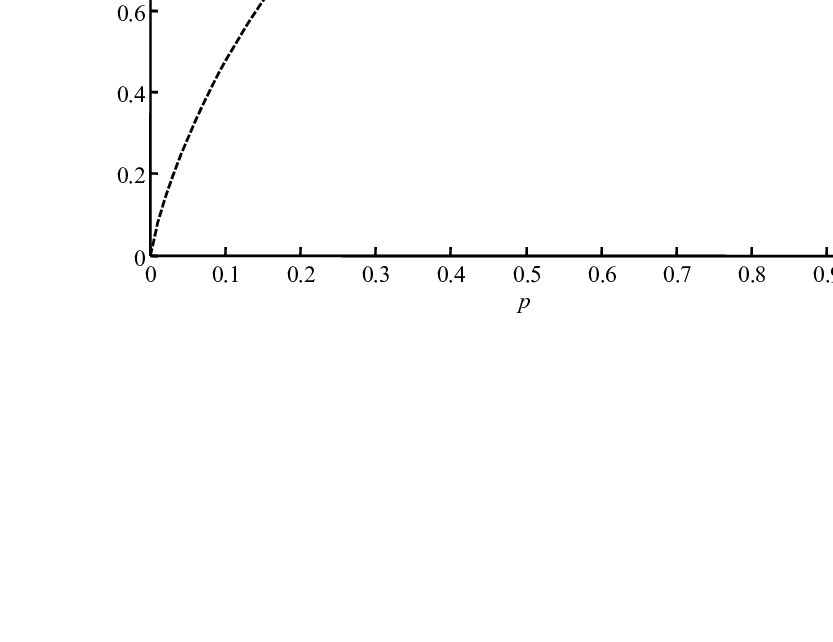
shows the sum-rates (24) and (25), demonstrating that, if $p$ is sufficiently small, namely if $p\lesssim 0.33,$ we have $R_{sum}^{\odot}(1)<R_{sum}^{\oplus}(1)$ and thus product side information is more informative than the sum, while for $p\gtrsim 0.33$ the opposite is true (and for $p=1,$ they are equally informative).

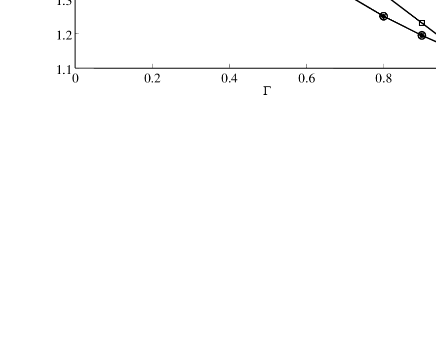
Considering a general cost budget $0\leq\Gamma\leq 1$, in order to emphasize the role of both data and control information for the system performance, we now evaluate the sum-rate attainable by imposing that the action $A$ be selected by Node 3 a priori, that is, without any control from Node 1. This can be easily seen to be given by [1]

This sum-rate will be compared below with the performance of the scheme in Proposition 1, in which the actions are selected based on both messages $(M_{1},M_{2})$, and that of Proposition 4, in which the actions are selected based only on message $M_{1}$.

Fig. 5 depicts the mentioned sum-rates²² 2 The sum-rate from Proposition 1 is calculated by assuming binary auxiliary variables $V_{1}$ and $V_{2}$ and performing global optimization. versus the action cost $\Gamma$ for $p=0.45$ and product side information. It can be seen that the greedy approach suffers from a significant performance loss with respect to the approaches in which actions are selected based on the messages received from one encoder or both encoders. It can be also observed that no gains are obtained by selecting the actions based on both messages. The fact that choosing the action based on the message received from Node 1 provides performance benefits can be explained as follows. If $X_{1}=0,$ the value of the side information is always $Y=X_{1}\odot X_{2}=0$ irrespective of the value of $X_{2}.$ Therefore, if $X_{1}=0,$ the side information is less informative than if $X_{1}=1$ and hence it may be advantageous to save on the action cost by setting $A=0.$ Consequently, choosing actions based on the message received from Node 1 can result in a lower sum-rate.

The scenario with sum side information is considered in Fig. 6 for $p=0.1$. A first observation is that, as proved in Appendix D, choosing the action based only on $M_{1}$ cannot improve the sum-rate with respect to the greedy case. This contrasts with the product side information case, and is due to the fact that $X_{1}$ is independent of the side information $Y$. Instead, choosing the actions based on both messages allows to save on the necessary communication sum-rate.

The problem of cascade lossy computing with causal observation costs at second user, illustrated in Fig. 3, is defined by the pmfs $p_{X_{1}X_{2}}(x_{1},x_{2})$ and $p_{Y|AX_{1}X_{2}}(y|a,x_{1},x_{2})$ and discrete alphabets $\mathcal{X}_{1},\mathcal{X}_{2},\mathcal{Y},\mathcal{A},\mathcal{\hat{X}}_{1},\mathcal{\hat{X}}_{2},$ as follows. The source sequences $X_{1}^{n}$ and $X_{2}^{n}$ with $X_{1}^{n}\in\mathcal{X}_{1}^{n}$ and $X_{2}^{n}\in\mathcal{X}_{2}^{n}$, respectively, are such that the pairs $(X_{1i},X_{2i})$ for $i\in[1,n]$ are i.i.d. with joint pmf $p_{X_{1}X_{2}}(x_{1},x_{2})$. Node 1 measures sequences $X_{1}^{n}$ and $X_{2}^{n}$ and encodes them in a message $M_{12}$ of $nR_{12}$ bits, which is delivered to Node 2. Node 2 estimates a sequence $\hat{X}_{1}^{n}\in\mathcal{\hat{X}}_{1}^{n}$ within given distortion requirements to be discussed below. Moreover, Node 2 encodes the message $M_{12}$, received from Node 1, and the locally available sequence $X_{2}^{n}$ in a message $M_{23}$ of $nR_{23}$ bits, which is delivered to node 3. Node 3 wishes to estimate a sequence $\hat{X}_{2}^{n}\in\mathcal{\hat{X}}_{2}^{n}$ within given distortion requirements to be discussed. To this end, Node 3 receives message $M_{23}$ and based on this, selects an action sequence $A^{n},$ where $A^{n}\in\mathcal{A}^{n}.$ The action sequence affects the quality of the measurement $Y^{n}$ of sequence $X_{1}^{n}$ and $X_{2}^{n}$ obtained at the Node 3. Specifically, given $A^{n}$, $X_{1}^{n}$ and $X_{2}^{n}$, the sequence $Y^{n}$ is distributed as in (1). The cost of the action sequence is defined by a cost function $\Lambda$: $\mathcal{A\rightarrow}[0,\Lambda_{\max}]$ with $0\leq\Lambda_{\max}<\infty,$ as in (2). The estimated sequence $\hat{X}_{2}^{n}$ with $\hat{X}_{2}^{n}\in\mathcal{\hat{X}}_{2}^{n}$ is then obtained as a function of $M_{23}$ and $Y^{n}$.

Estimated sequences $\hat{X}_{j}^{n}$ for $j=1,2$ must satisfy distortion constraints defined by functions $d_{j}(x_{1},x_{2},y,\hat{x}_{j})$: $\mathcal{X}_{1}\times\mathcal{X}_{2}\times\mathcal{Y}\times\mathcal{\hat{X}}_{j}\rightarrow[0,D_{\max}]$ with $0\leq D_{\max}<\infty$ for $j=1,2,$ respectively. A formal description of the operations at encoder and decoder follows.

References

- [1] H. Permuter and T. Weissman, “Source coding with a side information “vending machine”,” IEEE Trans. Inf. Theory, vol. 57, no. 7, pp. 4530–4544, Jul 2011.
- [2] A. El Gamal and Y. Kim, Network Information Theory, Cambridge University Press, Dec. 2011.
- [3] T. Weissman and A. El Gamal, “Source coding with limited-look-ahead side information at the decoder,”IEEE Trans. Inf. Theory, vol. 52, no. 12, pp. 5218–5239, Dec. 2006.
- [4] B. Ahmadi and O. Simeone, “Robust coding for lossy computing with receiver-side observation costs,” in Proc. IEEE International Symposium on Information Theory (ISIT 2011), pp. 2939-2943, July 31-Aug. 5, Saint Petersburg, Russia, 2011 (see also arXiv:1108.1535).
- [5] Y. Chia, H. Asnani, and T. Weissman, “Multi-terminal source coding with action dependent side information,” in Proc. IEEE International Symposium on Information Theory (ISIT 2011), pp. 2035-2039, July 31-Aug. 5, Saint Petersburg, Russia, 2011.
- [6] C. Heegard and T. Berger, “Rate distortion when side information may be absent,” IEEE Trans. Inf. Theory, vol. 31, no. 6, pp. 727-734, Nov. 1985.
- [7] A. Kaspi, “Rate-distortion when side-information may be present at the decoder,” IEEE Trans. Inf. Theory, vol. 40, no. 6, pp. 2031–2034, Nov. 1994.
- [8] K. Kittichokechai, T. J. Oechtering and M. Skoglund, “Source coding with common reconstruction and action-dependent side information,” in Proc. IEEE Information Theory Workshop, pp. 1-5, Dublin, Ireland, Aug. 2010.
- [9] K. Kittichokechai, T. J. Oechtering and M. Skoglund, “Secure source coding with action-dependent side information,” in Proc. IEEE International Symposium on Information Theory (ISIT 2011), pp. 1678-1682, July 31-Aug. 5, Saint Petersburg, Russia, 2011.
- [10] Y. Steinberg, “Coding and common reconstruction,” IEEE Trans. Inf. Theory, vol. 55, no. 11, pp. 4995-5010, Nov. 2009.
- [11] C. Choudhuri and U. Mitra, “How useful is adaptive action?,” in Proc. IEEE Globecom, Dec. 3-7, Anaheim, CA, 2012.
- [12] H. Asnani and T. Weissman, “On real time coding with limited lookahead,” submitted (arXiv:1105.5755).
- [13] S.-Y. Tung, “Multiterminal source coding,” Ph.D. Thesis, Cornell University, Ithaca, NY, 1978.
- [14] M. Gastpar, “The Wyner–Ziv problem with multiple sources,” IEEE Trans. Inform. Theory, vol. 50, no. 11, pp. 2762–2767, Nov. 2004.
- [15] B. Ahmadi, C. Choudhuri, O. Simeone and U. Mitra, “Cascade source coding with a side information "Vending Machine",” http://arxiv.org/abs/1207.2793.
- [16] S. Jana, “Alphabet sizes of auxiliary random variables in canonical inner bounds,” in Proc. Conf. Inf. Sci. Syst. (CISS), pp. 67-71, March. 18-20, Baltimore, MD, 2009.
- [17] A. H. Kaspi and T. Berger, “Rate-distortion for correlated sources with partially separated encoders,” IEEE Trans. Inform. Theory, vol. 28, no. 6, pp. 828–840, Nov. 1982.
- [18] A. B. Wagner, B. G. Kelly, and Y. Altug, “The lossy one-helper conjecture is false,” in Proc. Allerton Conf. on Communications, Control, and Computing, pp. 716–723, Sept. 30–Oct. 2, Monticello, IL, 2009.
- [19] T. Berger and R. Yeung, “Multiterminal source encoding with one distortion criterion,” IEEE Trans. Inform. Theory, vol. 35, no. 2, pp. 228–236, Mar 1989.
- [20] B. Ahmadi and O. Simeone, “Distributed and cascade lossy source coding with a side information “Vending Machine”,” http://arxiv.org/abs/1109.6665.
- [21] G. D. Forney Jr., “On the role of MMSE estimation in approaching the information- theoretic limits of linear Gaussian channels: Shannon meets Wiener,” in Proc. Allerton Conf. Communication, Control, and Computing, Monticello, IL, pp. 430–439, Oct. 2003.
- [22] Y.-K. Chia and T. Weissman, “Cascade and triangular source coding with causal side information,” in Proc. IEEE International Symposium on Information Theory (ISIT 2011), pp. 1683–1687, July 31-Aug. 5, Saint Petersburg, Russia, 2011.
- [23] J. Chen, X. Zhang, T. Berger, and S. B. Wicker, “An upper bound on the sum rate distortion function and its corresponding rate allocation schemes for the CEO problem,” IEEE J. Select. Areas Commun., vol. 22, no. 6, pp. 977–987, Aug. 2004.
- [24] G. Kramer, Topics in Multi-User Information Theory, Now Publishers, 2008.