Accelerated boundary integral method for multiphase flow in non-periodic geometries
Abstract
An accelerated boundary integral method for Stokes flow of a suspension of deformable particles is presented for an arbitrary domain and implemented for the important case of a planar slit geometry. The computational complexity of the algorithm scales as or ), where is proportional to the product of number of particles and the number of elements employed to discretize the particle. This technique is enabled by the use of an alternative boundary integral formulation in which the velocity field is expressed in terms of a single layer integral alone, even in problems with non-matched viscosities. The density of the single layer integral is obtained from a Fredholm integral equation of the second kind involving the double layer integral. Acceleration in this implementation is provided by the use of General Geometry Ewald-like method (GGEM) for computing the velocity and stress fields driven by a set of point forces in the geometry of interest. For the particular case of the slit geometry, a Fourier-Chebyshev spectral discretization of GGEM is developed. Efficient implementations employing the GGEM methodology are presented for the resulting single and the double layer integrals. The implementation is validated with test problems on the velocity of rigid particles and drops between parallel walls in pressure driven flow, the Taylor deformation parameter of capsules in simple shear flow and the particle trajectory in pair collisions of capsules in simple shear flow. The computational complexity of the algorithm is verified with results from several large scale multiparticle simulations.
Keywords:
accelerated boundary integral , confined , slit , non-periodic , capsule , red blood cells , microfluidics1 Introduction
Multiphase flow in confined geometries is ubiquitous in nature and technological applications. A very common example is blood flow in the microcirculation. Recall that blood is primarily a suspension of red blood cells (RBCs) in plasma, with the volume fraction of RBCs (hematocrit) typically ranging between in the capillaries and reaching as high as in large arteries [17]. The diameter of the blood vessels in the microcirculation, which includes the capillaries, arterioles and venules, is typically in the range [17], such that a discoidal RBC with a typical diameter and thickness of and respectively can be strongly to moderately confined. Therefore, any realistic computational study of blood flow in the capillaries must account for confinement. Other examples of technological interest where confinement effects are usually significant include multiphase flows in microfluidic devices [59]. Again, any realistic model must account for confinement in such problems. Given the importance of multiphase flows under confinement, or more generally speaking in non-periodic geometries, it is imperative to develop efficient and accurate computational techniques which faithfully represent the system under study, including the aspect of system size (meaning number of particles here). The algorithm presented herein has been motivated by our goal to study the class of problems described above. We next discuss some related previous efforts on the computational studies of multiphase flows under confinement.
Boundary integral based methods have emerged as a powerful tool for studying the flow behavior of multiphase systems in the limit of negligible Reynolds number, i.e. under Stokes flow conditions. Such methods have been employed in the past to study the flow behavior of a variety of particle types including drops, capsules, RBCs, and vesicles among others. Most of these prior implementations scale as , where is proportional to the number of degrees of freedom in the system. For a system with particles, each of which have been discretized into elements, the number of degrees of freedom in the system scales as . The scaling above assumes an iterative solution of the discretized system of equations, where the number of iterations is independent of ; a direct solution will result in a scaling of , while a system size dependent number of iterations with an iterative solution results in a scaling higher than ; the worst case scaling being . The scaling is usually prohibitive, such that it precludes a numerical study of large system sizes. It is therefore not surprising that many of the past studies have been limited to an number of particles.
To overcome these limitations, there have been several efforts to develop accelerated techniques, where an accelerated technique is assumed to give a scaling closer to the ideal , while being sufficiently accurate at the same time. These accelerated techniques employ either some variant of the particle-particle-particle-mesh (M) method [9], or the Fast Multipole Method (FMM) [20]. One of the earliest Stokes flow boundary integral implementation with acceleration was perhaps presented by Greengard et al. [18], who employed the FMM for acceleration in complex domains. Using the particle-mesh-Ewald (PME) method, Metsi [46] developed an accelerated implementation of the Stokes flow boundary integral method for her studies on two dimensional periodic suspensions of emulsions and foams. Zinchenko and Davis [64, 65] employed multipole expansion accelerated boundary integral method to study large number of drops in a periodic geometry under shear. Freund [16] used the smooth particle-mesh-Ewald method to study the motion of periodic suspensions of RBCs and leukocytes in two dimensions; this was later extended to three dimensions by Zhao et al. [63]. In the latter study [63], the effect of confinement was incorporated by explicitly discretizing the walls, which generally has unknown tractions and known no-slip velocity conditions. This explicit discretization is necessary because the periodic Green’s function does not inherently satisfy the no-slip condition on the walls. Additionally, the previous authors employed a staggered time integrator, such that the wall tractions and the particle surface velocities were not determined simultaneously; this is due to the large cost associated with their simultaneous solution. Another potential drawback with the periodic Green’s function is that it has a zero mean flow and a non-zero mean pressure gradient associated with it [22]. As a consequence, the pressure drop in the system is not directly a specified quantity, and must be solved for by varying the mean flow, which is a specified quantity [16, 63]. Note that many experiments on pressure driven flow have a specified pressure drop, and it is therefore desired to specify the pressure drop directly in numerical simulations without incurring additional computational costs. We also remark that the specified mean flow includes the flow outside the walls, as that is a part of the simulation box [63]; consequently, in such a method, neither the mean flow between the walls nor the pressure drop is a directly controlled quantity. Other recent work of possible interest is Rahimian et al. [52], where a FMM accelerated boundary integral method is presented. While this implementation was developed for an arbitrary domain, its applicability is restricted to two dimensional systems. In a subsequent article [62], the previous authors generalized their implementation to three dimensions, though only an unbounded domain was considered. At this point, it must be emphasized that all the prior accelerated implementations of the boundary integral method are based on either the free space Green’s function or the periodic Green’s function; in such a case, the boundaries of the confined domain are required to be explicitly discretized.
We next discuss previous boundary integral implementations employing the Green’s function for the geometry of interest. Such a Green’s function satisfies the appropriate boundary conditions at the domain boundaries; consequently, the unknowns at the domain boundaries, e.g. hydrodynamic tractions, do not enter the boundary integral equation. A popular geometry for which several boundary integral implementations have been developed is a slit – the region between two parallel walls. The Green’s function for this geometry has been provided by Liron and Mochon [42]. A boundary integral implementation based on this Green’s function was developed by Staben et al. [58] for rigid particles. This was later extended by Griggs et al. [21] for studies on drops in the same geometry. In a related work, Janssen and Anderson [27] also implemented a boundary integral method for drops between two parallel walls, though that was restricted to matched continuous and dispersed phase viscosities. This was later extended by Janssen and Anderson [28] to include non-matched viscosity problems. It is important to emphasize that none of these implementations are accelerated and have a computational cost of at least . Consequently, it is not surprising that all of the studies described above were limited to a few particles and are thus not suitable for studying suspension dynamics.
We now briefly discuss examples of other numerical techniques employed in the literature for studies on the flow behavior of particles under confinement. One such simulation technique is the immersed boundary method, which has been employed, e.g. by Doddi and Bagchi [11] and Pranay et al. [51], for studies on capsules in a slit. Another popular technique is the lattice-Boltzmann method. As an example, MacMeccan et al. [44] developed a coupled lattice-Boltzmann and finite element method to study deformable particles, which included studies under confinement. A somewhat related algorithm is the multiparticle collision dynamics, which has been used by, e.g., Noguchi and Gompper [48] to study RBCs and vesicles in capillaries. The ideal computational cost of all the above numerical techniques is . Finally, Swan and Brady [60] have developed an accelerated Stokesian dynamics method for rigid spherical particles in a slit that uses ideas related to those presented here and scales as .
In the present study, we develop an accelerated boundary integral method for multiphase flow in an arbitrary geometry and implement it for a slit geometry as shown in Fig. 1. The computational complexity of this algorithm scales as or depending on the specific numerical scheme employed. The latter scaling of is associated with the use of fast Fourier transforms (FFTs) if one or more directions have periodic boundary conditions, though that is not a requirement of our method. In the present effort, we provide a detailed description using the example of the slit geometry; its extension to other geometries is straightforward. The acceleration in our method is provided by the use of General Geometry Ewald-Like Method (GGEM) [24]. The choice of GGEM as the acceleration technique necessitates the use of an alternative boundary integral formulation in which the velocity field is expressed solely in terms of a single layer integral [50]; its unknown density is obtained from a second kind integral equation involving the double layer integral. The resulting single and double layer integrals are computed efficiently employing the GGEM methodology, which results in the aforementioned favorable scaling of or .
The organization of this article is as follows. In Sec. (2), we provide a brief overview of the GGEM accelerated boundary integral method and also discuss some of the limitations of the current implementation. Following this, in Sec. (3), we present the boundary integral formulation and discuss its numerical implementation using GGEM. In Sec. (4), we present the procedure to compute the hydrodynamic traction jump at a particle surface using the example of a capsule with a neo-Hookean membrane. The solution procedure for the discretized boundary integral equation is presented next in Sec. (5). An extensive validation of our method is presented in Sec. (6). Lastly, in Sec. (7), we present results from several large scale multiparticle simulations and verify the computational complexity of our algorithm.
2 Overview of the current work
We summarize here some of the key aspects of the present work. Each of these points are discussed further later in the article.
- 1.
The general geometry Ewald like method (GGEM) employed in the current work for acceleration essentially yields the geometry-dependent Green’s function and other associated quantities. This work is a first instance of an accelerated boundary integral method based on the geometry-dependent Green’s function. Prior implementations have employed either the free-space Green’s function (in case of FMM accelerated methods) or the periodic Green’s function (in case of PME accelerated methods).
- 2.
The GGEM methodology decomposes the overall problem into a local problem and a global problem, essentially by splitting the Green’s function into local (singular but exponentially-decaying) and global (smooth but long-ranged) parts. The implementation of the local problem is similar to that of the traditional boundary integral method. However, since the local Green’s function decays exponentially with distance from the source of the singularity, distant elements are not coupled and the local solution can be obtained in operations.
- 3.
The global problem involves solving a single phase Stokes equation in the domain of interest with known boundary conditions and with a known smooth distribution of force densities. It is in this problem that the coupling between distant elements appears. In solving the global problem, one is not concerned with the particle interfaces, or the different viscosity fluids present inside and outside the particle (if that is the case in the original problem). This major simplification allows the use of a wide variety of fast and accurate numerical techniques present in the literature for the solution of Navier-Stokes equation in an arbitrary domain. All these methods, including those based on finite difference, finite volume, finite element, and spectral methods are suitable here [6, 7, 12, 14]. In addition, various fast and efficient implementations of Navier-Stokes solvers on GPUs and distributed memory systems are readily available [23, 61].
- 4.
We present a spectral Stokes flow solver for the global problem in a slit geometry, which, as indicated in the introduction, is one of the most widely-studied confined geometries studied in the literature. This solver employs a Fourier-Chebyshev Galerkin method in conjunction with the influence matrix approach [7]. The unknown coefficients of the Fourier-Chebyshev series expansion are computed with a direct algorithm – no iterations are necessary here, as would be the case with FMM or PME accelerated methods in a slit.
The implementation of the methodology presented in this paper also has some limitations. An important limitation of the current implementation concerns the evaluation of the near singular integrals – these integrals arise when the gaps between the particles become very small, and, if not treated appropriately, may cause the simulations to diverge. In the present work this is alleviated by requiring that the minimum interparticle gap in the system be always maintained above a specified value; this is achieved by the use of an overlap correction procedure in an auxiliary step. There are several other minor limitations of the current implementation. For example, we currently use linear elements to discretize the particle surface. It may be beneficial to employ higher order discretizations, like a spectral discretization, which could be particularly helpful for the accurate evaluation of the near singular integrals. In this paper results are reported only for a slit geometry. It will be appropriate to develop efficient implementations of the our methodology for other geometries like a cylinder. It must be emphasized that none of the above limitations are inherent to our methodology and we hope to address these in future efforts.
3 Problem Formulation and Implementation

3.1 Boundary integral equation for fluid motion
We consider a three-dimensional suspension of deformable particles (e.g. fluid-filled capsules) as shown in Fig. (1), where both the suspending fluid and the fluid enclosed by the particles are assumed to be Newtonian and incompressible. The viscosity of the suspending fluid is taken to be , while the viscosity of fluid enclosed by capsule is taken to be , such that is the viscosity ratio of the interior and the exterior fluid for this particular capsule. The Reynolds number for the problem is assumed to be sufficiently small that the fluid motion is governed by the Stokes equation. Under these assumptions, one may write the velocity at any point in the domain with an integral expression involving only the boundary of the particles [50]. We first introduce the formulation that is most commonly used,
| (1) |
where is the fluid velocity at a point lying on the boundary of particle (i.e. , denotes the surface of particle ), is the undisturbed fluid velocity at the point , is the hydrodynamic traction jump across the interface [50], and the sums are over all the particles in the system. The Green’s function and its associated stress tensor are denoted by and respectively in the above equation, and integrals involving them as the kernel are typically referred to as the single layer integral and the double layer integral respectively [30, 50]. From here onwards, a principal value of the double layer integral over a part of the boundary is assumed whenever the target point lies on that boundary. For example, in the above equation, the double layer integral over is assumed to denote the principal value when . A crucial aspect of the above formulation is that the Green’s function and associated stress tensor are taken to satisfy the boundary conditions imposed at the system boundaries, so the integrals above only involve the internal (interfacial) boundaries; if the Green’s function for any other geometry is employed (e.g. periodic), additional integrals over the domain boundaries arise in Eq. (1).
The above form of the boundary integral equation (1), using the free space Green’s function (the Oseen-Burgers tensor) or the Green’s function for a triply periodic domain given by Hasimoto [22] is widely used in the literature and is the basis for numerous numerical implementations, including the references cited in the introduction. However, for reasons that will be discussed shortly, this form is not amenable to numerical solution by an accelerated method in an arbitrary domain when using the Green’s function for that domain. In the present effort, therefore, we employ an alternative formulation in which the fluid velocity is expressed solely in terms of the single layer integral with density as follows:
| (2) |
The single layer density satisfies (for )
| (3) |
where is defined as
| (4) |
while is the traction at a given point (computed with the suspending fluid viscosity ) due to the stress generated in the fluid corresponding to the undisturbed flow (see B for examples). In A, this formulation is derived from the Lorentz reciprocal theorem for the case of a single particle. This derivation follows closely the approach outlined in Chap. (5) of Pozrikidis [50] and is provided here for completeness.
We now clarify the motivation for employing Eqs. (2) and (3) rather than the more commonly employed formulation in Eq. (1). We begin by noting that the first argument of and denotes the field (target) point of the functions, while the second argument denotes the location of the pole (source) of the singularity that drives the flow. A close look at Eq. (1) reveals that the operand of , , is a function of the position of the pole of the singularity () and that the field point of the tensor is same as the target point of the overall boundary integral equation (). In other words, the operand of is independent of its target point, and consequently the same collection of point forces can be used to compute the velocity at any target point. This requirement is essential to any accelerated method, as in such methods a part of the calculation gives the velocity (or other relevant quantities) simultaneously at all target points (e.g., boundary element nodes) due to all the singularities present in the system. This is possible only if the operands of the singularities are independent of the target points of the singularities, and instead are functions of the location of the pole of the respective singularities.
With this aspect clarified, it is seen that this important condition is not satisfied for the double layer kernel in Eq. (1) as its multiplicands and are functions of its target point . Also note that no general relationship exists that would allow one to switch the location of the pole and the field points in . (This is possible for , since, by self-adjointness, [50]). Hence the above formulation (1) is not suitable for our purposes here, though it can still be used for problems in which the viscosity ratio is unity, as the double layer integral vanishes in such a case [51]. In contrast, in the formulation employed in this work (Eqs. 2 and 3), the multiplicand of both and is a function of the location of the source point . Hence, it is amenable to numerical solution by an accelerated method.
We now describe the fast computation of the velocity and pressure fields due to a collection of known point forces, which is closely related to the problem of computing the Green’s function and its associated stress tensor in the geometry of interest. Later in Secs. (3.4) and (3.5), we employ this technique to compute the single layer and double layer integrals.
3.2 GGEM Stokes flow solver for a collection of point forces
Consider the velocity field and the pressure field due to a collection of point forces, such that the strength and location of the point force are given by and respectively. The velocity and pressure fields above are obtained from the solution of the Stokes and the continuity equation as shown below:
| (5a) |
| (5b) |
and subject to given boundary conditions on the system boundary . By definition, the above velocity and pressure fields along with the associated stress tensor can be written in terms of a Green’s function , its pressure vector and stress tensor as
| (6a) |
| (6b) |
| (6c) |
The stress tensor in the above equation is obtained from and from the Newtonian constitutive equation
| (7) |
A close look at the boundary integral equations (2) and (3) shows that to evaluate the integrals we do not explicitly need the Green’s function and its stress tensor but only their products with the density . Put simply, our end goal is to quickly find in time or the velocity and the stress tensor due to a given set of point forces – explicit construction of and are not necessary.
One of the attractive features of the method presented here lies in the fact that it is applicable to an arbitrary geometry. For simplicity and considering the interest of the present work, we provide a detailed discussion only for a slit geometry (see Fig. 6); generalization of the formalism for an arbitrary geometry is straightforward [25]. For the present slit domain, there is a no slip boundary condition at the two rigid walls at and , while periodic boundary conditions are assumed in the other two directions and , with spatial periods and , respectively.


To achieve the computational complexity of alluded to above, we employ the general geometry Ewald like method (GGEM) [24] for computing the velocity and stress fields due to a given collection of point forces. We briefly describe GGEM next. In the GGEM methodology, the Dirac-delta density in Eq. (3.2) is expressed as the sum of a smoothly varying quasi-Gaussian global density characterized by a “splitting parameter” and a second local density (see Fig. 2). Here is a position vector relative to the pole of the singularity, . The above global and local densities are respectively given by the following expressions:
| (8a) |
| (8b) |
where represents a length scale over which the delta-function density has been smeared using the quasi-Gaussian form above, and consequently it also represents the length scale beyond which both the global and the local densities are effectively zero. It is important to emphasize that the total density remains a -function, i.e. . The motivation for this particular splitting of the -function density into and will be obvious below.
We next consider the solution of the Stokes and continuity equation with the above two force densities as forcing functions. The solution driven by the local density, , , and (velocity, pressure, and stress respectively) will be referred to as the local solution, and satisfies the local problem
| (9a) |
| (9b) |
This equation will be solved in an unbounded domain, i.e. the solution decays to zero at infinity. The solution , , and driven by the global density will be referred to as the global solution, and satisfies the global problem
| (10a) |
| (10b) |
The boundary conditions for the global problem are set so that the total velocity field satisfies the specified boundary conditions for the overall problem. Once the local and the global solutions are known, the solution to the overall problem is obtained as
| (11a) |
| (11b) |
| (11c) |
We next discuss the solution procedures for the local and the global problems.
3.2.1 Local solution
Consider first the local problem. The solution to this problem, , , and is expressed by a set of equations similar to that in Eqs (3.2), which, for the simplicity of nomenclature, is called the local Green’s function and its associated quantities. In short, we append the superscript to the previously defined quantities to denote the solution associated with the local density as the forcing function, and these are given by the following:
| (12a) |
| (12b) |
| (12c) |
where , while . The velocity and stress fields are then obtained as:
| (13a) |
| (13b) |
The solution in Eq. (3.2.1) has been obtained with free-space boundary conditions, i.e. all of them decay to zero at infinity. In other words, the local solution is independent of the geometry of interest. The violation of the boundary condition requirements of the domain by employing free space boundary conditions above will be corrected by appropriately choosing the boundary conditions for the flow problem associated with the global force densities as the forcing function.
An important observation at this point is that the local solutions in (3.2.1) are short ranged, decaying approximately as . Consequently, the contribution from the local solution can be neglected beyond a length scale from the origin of the corresponding local density. In this work, this cutoff length was taken as throughout. The near neighbor list required for the efficient computation of the local solution is generated by the cell-linked list algorithm [1].
It is important to point out that the in Eq. (3.2.1a) has the same functional form as the real space term in the periodic Stokeslet (Green’s function) provided by Hasimoto [22]. In other words, Hasimoto’s solution for the periodic Stokeslet can also be obtained by first splitting the -function density into the local and global densities as in Eq. (3.2); the local problem is then solved as described above, while the global problem is solved with a Fourier Galerkin method with the appropriate assumptions described in Hasimoto [22]. Since PME accelerated methods (e.g. [34]) for Stokes flow employ the periodic Stokeslet given by Hasimoto [63], this observation illustrates a connection between PME like methods and GGEM. A very important distinction, though, is that the performance of PME like methods is tied to the use of discrete Fourier transforms and thus periodic domains, which is not the case with GGEM (discussed below) and hence the latter’s much broader applicability.
3.2.2 Global solution
We now describe the solution to the global problem, i.e. the flow problem associated with the collection of global force densities. We first discuss the boundary conditions for the global problem. As was mentioned earlier, the overall solution for a given collection of point forces is the sum of the corresponding quantities from the local and the global solutions, see Eq. (3.2). It is obvious that the same should be true for boundary conditions. Consequently, to satisfy any type of boundary condition (e.g. Dirichlet) at an arbitrary location, we set the boundary condition for the global part so that its sum with the known contribution from the local part (above) adds up to the required value. Again, we employ the example of the slit geometry, noting that this scheme is equally applicable to other geometries. To satisfy the no-slip condition at the two rigid walls of the slit, we require the following at and :
| (14) |
Note that in the present formulation the static no-slip condition is always imposed at the rigid walls for computing the velocity field due to the Green’s function (or point forces). This is true even in problems where the walls may not be at rest, a common example being simple shear flow. The effect of the undisturbed flow enters the boundary integral equation via and in Eqs. (2) and (3). To satisfy the periodic boundary conditions in and directions, we impose equivalent periodic boundary conditions in the global calculation. As far as the local solution is concerned, we require that it decays to a negligible value over a length scale equal to half of the spatial period in and directions or smaller: i.e. and . Given the above choice , we require that . This fact, coupled with the minimum image convention [9] employed in the computation of the local solution ensures its periodicity.
Before proceeding further, we note that, in general, two subtleties arise in considering the behavior of the global solution near boundaries. The first is the issue of boundary shape. In the present work we take the boundary to be smooth on the scale of the suspended particle size. If that is not the case, it will be necessary to resolve the length scales of the boundary roughness. For such a boundary it might be convenient to revert to a conventional accelerated method and explicitly discretize the boundary. Alternately, in the present context, the global solution could be obtained using a locally-refined mesh near the domain boundary to capture its features (see, e.g. Fard et al. [13]), without destroying the scaling of the method with the number of suspended particles.
Another issue arises in principle if a particle very closely approaches a (smooth) boundary. This does not arise in the context of the present application as deformable particles migrate away from solid surfaces in shear flow due to the hydrodynamic dipole interaction between the particle and the wall [57]. Nevertheless, it can happen in principle and leads to the situation where the boundary condition for the global problem that must be satisfied becomes nearly singular. This is because, at a no-slip boundary, we require and a point force a distance away from the boundary leads to a local velocity of on the boundary. This situation can be addressed by adding the image system for a plane wall [5] (and splitting it into local and global parts), in which case the effects of the singularities cancel on the wall. See Swan and Brady [60] for a related discussion in the Stokesian dynamics context.
Having discussed the boundary conditions for the global problem, we turn to the solution procedure of the Stokes and the continuity equation with the given collection of global force densities as the forcing function; see Eq. (3.2). For an arbitrary geometry one may employ any desired discretization scheme for the solution of the global problem. If a finite difference or a finite element scheme is used, then the solution can be obtained at a cost of when the resulting sparse matrix equations are solved iteratively with proper preconditioners; the multigrid preconditioner for Stokes flow is an attractive choice [12, 56]. Section 7.2 contains further discussion of the scaling of computation time with problem size. For the slit problem of interest here, past work [25, 51] employed discrete Fourier series approximation in the periodic and directions, while a second order finite difference discretization was employed in the wall normal direction. In the present work, we develop a fully spectral solution procedure by employing the discrete Chebyshev polynomial approximation [6] in the wall normal direction, while the discrete Fourier series approximation is used in the periodic and directions. For example, the -component of the global velocity in Eq. (3.2) is expressed as
| (15) |
where is the Chebyshev polynomial of the degree [6], represents the mapping from to : , while , , and respectively denote the number of terms (modes) in the corresponding series approximation. Similar expressions are written for other components of the velocity and the pressure. An important implication of this representation, particularly with regard to the pressure, is that the pressure drop associated with this point force solution is always zero over the spatial period of the domain, while the mean flow is (in general) non-zero. This ensures that the pressure drop obtained from the boundary integral method always equals the pressure drop specified in the imposed bulk flow (i.e. in the absence of the particles). Returning to the expression in Eq. (15), we note that the use of the Fourier series approximation in and directions ensures that the periodic boundary conditions in these directions are inherently satisfied. The Chebyshev polynomials, on the other hand, do not automatically satisfy the boundary conditions in the wall normal direction; the satisfaction of these boundary conditions was accomplished by employing the tau method [6, 49]. In the tau method, the equations for the highest two modes in the series approximation are replaced by equations representing the two boundary conditions; see, e.g., Canuto et al. [6] or Peyret [49] for details. An attractive feature of the discrete Chebyshev polynomial approximation is that FFTs can be used for rapidly transferring information from the physical to spectral space and vice-versa [7]. A major drawback, though, with solving differential equations with Chebyshev polynomial approximation is that the differentiation matrix is full in both the spectral and the physical space [49] (in contrast, the Fourier differentiation matrix is diagonal in the spectral space). Due to the full nature of the Chebyshev differentiation matrix, a straightforward implementation for solving the Stokes flow problem will lead to an method. For the incompressible Stokes flow problem here, though, an alternate approach exists in which the solution to the Stokes equation is obtained from the solution of a series of Helmholtz equations [7]. In this case, with a little manipulation, a quasi-tridiagonal system of equations results, for which a direct algorithm exists [49]. This approach for solving the incompressible Stokes equation, or more generally the incompressible Navier-Stokes equations, is popularly known in the literature as the Kleiser-Schumann influence matrix method [7]. A detailed discussion of this approach including the equations being solved and their respective boundary conditions is presented in C. Here we only sketch out the main computational aspects of this approach. To begin, each of variables appearing in the Stokes and the continuity equation are expanded in a truncated Fourier series in and directions; see, e.g., Eq. (15). These expressions are then substituted in the Stokes and the continuity equations. Subsequently, by the application of the Galerkin method, a set of coupled ordinary differential equations (ODE) in is obtained for each of the Fourier modes of all the unknown variables (velocity components and pressure). These coupled ODEs are solved with the Chebyshev-tau influence matrix method, which involve Chebyshev transformations, quasi-tridiagonal matrix equation solves, and inverse Chebyshev transformations in that order. The solution thus obtained yields the Fourier coefficients of the velocity components and the pressure. An inverse Fourier transform then leads to the solution for the velocity and the pressure in the physical space. The computation of the stress tensor requires the derivatives of the velocities; these differentiations are performed in the transform space [6, 49]. All of the above Fourier and the Chebyshev transforms along with their inverse transforms are performed using the FFT algorithm. Thus, the asymptotic computational cost of the solution procedure for the global problem scales as , where . Assuming (see Sec. 7.2), we obtain the asymptotic computational cost of the global solution as . A further discussion on the computational complexity of the algorithm is provided in Sec. (7.2).
We next introduce some of the important parameters associated with this solution procedure. Associated with each of the and Fourier modes, there are and equispaced trapezoidal quadrature points; the corresponding spacings are denoted by and . Similarly, associated with the Chebyshev polynomials, there are Chebyshev Gauss-Lobatto quadrature points, the of which is given by ; the mean mesh spacing in this case is denoted by . Unless otherwise mentioned, the mean mesh spacings in all three directions are kept equal in simulations, i.e. . For computing any of the above transforms, the value of the corresponding physical variable is required only at the corresponding quadrature points. Likewise, as is customary, the final solution for the velocity, pressure and stress are also computed only at these quadrature points. This last step is essential in maintaining the optimal computational complexity of alluded to above. The velocity and stress at any point not on the mesh is obtained via interpolation; here we employ order Lagrange interpolation for which the error decays as , where is the characteristic mesh spacing. The error, therefore, is expected to decay exponentially fast with the number of modes for any point on the mesh, while it is expected to decay as for any point not on the mesh. It is appropriate to pointÊout here that exponential convergence of the solution is possible even at a non-mesh point while maintaining the computational complexity of – this can be achieved by employing the basic principles of non-uniform FFT calculations; see, e.g., [19, 40] for details.


3.2.3 Convergence of the GGEM solution
We demonstrate next the convergence behavior of the GGEM Stokes flow solution presented above. It will be helpful to begin this section with a discussion of various sources of error in the solution procedure. It should be obvious that the overall error in the solution results from errors in both the local and the global solution procedures. The error in the local solution arises due to its truncation beyond a distance of from the source of the singularity – this error scales as (Sec. 3.2.1, [40]). Typically, we set , which is expected to result in an error of . Smaller error in the local solution can be obtained by increasing the value of . The error in the global solution has three different sources. The first source of error is the truncation of the Fourier-Chebyshev series expansion at some finite number of modes; see Eq. (15). The error due to this truncation is expected to decay exponentially fast on the mesh points with the parameter – this convergence rate results due to the spectral nature of the global solution procedure employed here. For other solution procedures, such as a finite difference scheme [25, 51], an algebraic convergence with the parameter will be obtained. Next, for any point not on the mesh, the global solution has to be obtained by interpolation from nearby mesh points, which introduces an additional error scaling as in the current work. Lastly, there is also an error associated with the assignment of the global force density on the mesh points – this is required for computing its Fourier and Chebyshev transforms. The global density decays approximately as with distance from the origin of the density (Eq. 3.2a). Therefore, just like the local solution, we truncate the global density beyond a distance of from the origin of the singularity. It is expected that the error due to this truncation will scale as . Again, a smaller truncation error can be obtained by setting a larger value of – in such cases the cost associated with the global force density assignment on the mesh points can be large and the fast Gaussian gridding algorithm [19, 40, 41] is recommended.
Having discussed the various sources of errors in the solution procedure, we turn to verifying the expected convergence behavior with a test problem. In this test problem, we compute the velocity field due to a point force in a slit of side , i.e. . The point force is located at coordinates , while its strength is given by . The velocity due to this point force will be computed at two target points. The first target point is located at the center of the box , which is easy to maintain on a mesh point, while the second target point is a randomly chosen point with coordinates , which is unlikely to be a mesh point. In this test study, we will keep the value of fixed at , while the value of ( is a constant) and the mean mesh spacing will be varied. Figure (3a) shows the relative error in the component of the velocity as a function of for several different values of for the first target point, while the same is shown for the second target point in Fig. (3b). The data points in these plots were obtained by varying between and , while the solution computed with and (i.e., ) is taken as the reference for computing the relative error. Focusing first on Fig. (3a), we observe an exponential convergence in the velocity with increasing , though it eventually levels off at a value depending on the choice of . For the typical value of , an error of is obtained. We next focus on the velocity convergence at the second target point (Fig. 3b), which is a non-mesh point. For the choice , we again observe an exponential convergence initially with increasing that eventually levels off at approximately the same value as for the first target point. For higher values of ( and ), we observe an exponential convergence initially, though a convergence rate scaling as is observed at higher values of . The latter convergence rate results from interpolation errors becoming dominant at higher values of . We also note that an exponential convergence is observed only when the length scale of the global force density is well resolved by the numerical mesh. Since the length scale of the global force density is represented by , the requirement for an exponential convergence is quantitatively expressed by the condition (i.e. ). This requirement on the mesh spacing is more easily appreciated if one interprets as the number of mesh points per unit smearing length represented by ; therefore the larger is , the higher is the resolution of the numerical scheme. Based on extensive numerical tests presented in this paper, is a recommended value as convergence was usually observed at this resolution.


3.3 Surface discretization
Having described the procedure for the fast computation of the velocity and the stress fields associated with a given collection of point forces, we now turn to the numerical solution of the boundary integral equation introduced in Sec. (3.1). In this section, we describe the discretization of the particle’s surface into elements along with the basis functions employed over each element. Following this, we describe the numerical implementation of the single and the double layer integrals present in the boundary integral equation. It should be emphasized that accelerated approach described here is not limited to the specific surface discretization used here; this discretization was chosen because it has been used in past works on the dynamics of fluid-filled elastic capsules and drops in flow [11, 31, 51, 43, 64].
In the present work, the surface of a capsule is discretized into triangular elements. Triangulation of a sphere is achieved by mapping the vertices of an icosahedron, which has 12 vertices and 20 triangular faces, to the surface of the inscribed sphere [54]. This procedure will, therefore, give 20 elements on the surface of the sphere. Further refinement is obtained by subdividing each triangular face of the icosahedron recursively into 4 equal triangular elements, with all the vertices (and consequently the elements) again being mapped to the surface of the inscribed sphere as described above. The number of elements () and the number of vertices () obtained by this procedure can be expressed as and , where is the level of refinement ( corresponds to the original icosahedron). Note that the 12 original vertices of the icosahedron have a coordination number 5, while the remaining vertices have a coordination number of 6. As an example, a sphere subdivided into elements with vertices is shown in Fig. (4(a)).
3.3.1 Basis functions over elements
Linear basis functions are used over each element. All computations over a triangular element is performed by mapping to or from the parent triangle [26]. The parent triangle employed in this work is shown in Fig. (4(b)), where and denote the natural coordinates. The basis functions associated with the nodes 1, 2, and 3 are respectively given in natural coordinates by
| (16a) |
| (16b) |
| (16c) |
As an example, the position vector as a function of natural coordinates is obtained as
| (17) |
where , , and are the real space positions of vertices 1,2, and 3 respectively. The same procedure is employed to obtain the value of any physical variable (e.g. velocity) at coordinates () over the domain of the parent triangle.
3.4 Single layer integral
Let the single layer integral over the surface be denoted by
| (18) |
where is the single layer density, while is assumed to represent the velocity at point . In order to employ GGEM as discussed in Sec. (3.2) to compute the above integral, we write this equation in the form
| (19) |
where represents the volume of the domain and is the three dimensional Dirac delta function. It is easy to see that both the expressions for in Eqs. (18) and (19) are identical. Next, we write the Dirac-delta function as a sum of the local and the global density introduced in Sec. (3.2); see Eq. (3.2). Consequently, we have
| (20) |
Next, we separate the integrals associated with the local and global densities, and write the contribution due to the local density as
| (21) |
It is easy to see that the above integral can be written as
| (22) |
where has been defined in Eq. (3.2.1). This follows from the fact that the local Green’s function can also be constructed by the superposition of Green’s function weighted by the density , i.e.
| (23) |
It is important to emphasize that the domain was assumed to be unbounded in arriving at Eq. (23). This is always the case for the local problem as discussed in Sec. (3.2); any error in the boundary condition introduced due to this assumption will be accounted for in the global calculation. Next, consider the contribution from the global density in Eq. (20), which we write as
| (24) |
It can shown that satisfies
| (25a) |
| (25b) |
where the density is given by
| (26) |
The boundary condition for the global solution comes from the known local solution ( for at the domain boundary) and the given overall boundary conditions, such that the sum of the local and the global solution satisfies the overall boundary condition; see Sec. (3.2). Having expressed the single layer integral in a form suitable for its computation with the GGEM technique, we next describe its numerical implementation. This includes the numerical solution of the local problem represented by Eq. (22) and the global problem represented by Eq. (3.4).
3.4.1 Local contribution
We first consider the contribution from the local Green’s function to the velocity at a given point , which typically is one of the nodes of the elements. We discretize the surface integral in Eq. (22) as
| (27) |
where the summation is over all the triangular elements present in the system, while denotes an integral over the element . For convenience, all the integrals are performed over the parent triangle. To accomplish this, we write the above equation as
| (28) |
where the differential area element has been replaced by its equivalent expression
| (29) |
As noted earlier, the value of any quantity can be obtained at coordinates by the usual interpolation from the corresponding values at the nodes of the triangle, e.g. see Eq. (17). The double integral in Eq. (28) is evaluated using the product of two one-dimensional Gauss-Legendre quadrature rule (one for and the other for ). This proved competitive in terms of computational cost for a given accuracy with Gaussian quadrature rules available for a triangular element [26], perhaps due to the fact that the integrands are not polynomials. In most cases a 4x4 product rule is found to be sufficient for accurate integration over a triangular element. In addition, if the vertex at which the velocity is being computed is a member of the triangular element over which the integration is being performed, then the integral in Eq. (28) over the parent triangle is further transformed to polar coordinates [54]. This transformation makes the integrand non-singular and hence ensures sufficient accuracy with the same low order product integration rule discussed above. Lastly, we note that for computing the contribution to velocity at any given point due to the local Green’s function, only triangular elements within a distance of from the point need to be considered (typically, ). This is justified due to the exponentially decaying contribution from the integral over an element at separations larger than from the point of interest. As mentioned in Sec. (3.2.1), the near neighbor list required for the local calculation is generated in time via the cell-linked list method [1].
3.4.2 Global Contribution
Our goal here is to find in Eq. (3.4), for which we need to compute the integral in Eq. (26). We being by discretizing the integral in Eq. (26) and write it as
| (30) |
The above integral can be evaluated with any desired quadrature rule, though, due to the smoothly varying nature of the integrand a simple trapezoidal rule proves sufficient. Note that the trapezoidal integration rule essentially reassigns the contribution from the surface of the triangular element to its three vertices in equal proportions. Consider first the integral over an element in Eq. (30), which as per the trapezoidal rule is expressed as a sum of contributions from its three vertices as
| (31) |
where is the area of the triangular element , denotes the vertex number of the given element , denotes the coordinate of the vertex of the triangular element , and denotes the density at due to the integration over the element only. The term in the parenthesis in Eq. (31) can be considered as the strength of the global density at the node due to the element ; by summing it over all the elements to which a given node belongs (let us say that this node is globally represented by ), one obtains the total strength of the global density at this node, say . The overall density at a point is then obtained by adding contributions from all the nodes present in the system,
| (32) |
where is the total number of nodes in the system. We also note that due to the exponentially decaying nature of as a function of distance from , we consider only those nodes for computing the density at a point which are within a distance from it. Once is evaluated, we solve the set of equations in (3.4) using the procedure described in detail in Sec. (3.2). This gives us at the mesh points. The velocity at any point not on the mesh is obtained using order Lagrange interpolation. Once is known, the overall single layer integral is obtained as:
| (33) |
3.5 Double layer integral
We now describe the evaluation of the double layer integral. We denote the double layer integral over a surface (similar to that in Eq. 3) by
| (34) |
If we define a stress tensor () as (note that one needs to multiply it by to get units of stress)
| (35) |
then we have the following relationship between and ():
| (36) |
The motivation for introducing the stress field () in Eq. (35) should be clear now, as it is the stress field associated with the following velocity field
| (37) |
As described in the previous section (3.4), we write the above velocity field as the sum of a local and global velocity fields, and denote the corresponding stress fields by () and () respectively. Using (36), we obtain the corresponding local and global contributions to the double layer integral as
| (38a) |
| (38b) |
We describe the computation of the global contribution to the double layer integral first, as it is a straightforward extension of the procedure presented in Sec. (3.4). This will be followed by a discussion of the procedure for computing the local contribution to the double layer integral.
3.5.1 Global contribution
Here we describe the procedure to compute the global contribution to the double layer integral. Consider the global velocity field and the pressure field associated with the global force density ; see Eq. (3.4). The procedure to compute the velocity and pressure field for this global distribution of density has been discussed in detail in Sec. (3.4). Once these are known, one can obtain the stress field from the usual Newtonian constitutive equation as
| (39) |
As was mentioned in Sec. (3.2), the differentiations required in the above expression are performed in the transform space [6, 49]; consequently, the stress field is known with spectral accuracy at the mesh points. Once the stress tensor is obtained at the mesh points, the stress at the nodes of the elements are obtained using order Lagrange interpolation. Lastly, is obtained from Eq. (38b).
3.5.2 Local contribution
Consider the velocity field due to the local density, which is written as
| (40) |
It is trivial to show that the stress field associated with the above velocity field is given by the following
| (41) |
and consequently the local contribution to the double layer integral is given by
| (42) |
The above integral is discretized in the same fashion as in Sec. (3.4), and is written as a sum of integrals over the triangular elements. Again, as in Sec. (3.4.1), all the integrals are performed over the parent triangle as follows
| (43) |
The integral in the above equation is performed with the product of two one dimensional Gauss-Legendre quadrature rule; see Sec (3.4.1) for details. In addition, when the vertex at is a member of the element over which integration is performed, the integrand is singular and requires special treatment. At this point it is worth noting that the double layer integrand has the same singularity as the single layer integral [47], as for small . So in principle one may employ the polar coordinate transformation to regularize the singular double layer integral. In practice, because we employ flat elements, the condition is not valid. Note that the normal vector at any given vertex is taken as the area averaged normal vector of triangles to which it belongs, from which it follows that the numerical double layer has a singularity. This stronger singularity can be avoided by employing surface elements that yields a continuously varying normal vector such as splines [36].
In the literature, desingularization of the double layer integral is usually achieved by singularity subtraction [50]. This desingularization scheme is also applicable for the current formulation (34), though this procedure will require 9 times the computational effort of performing the double layer integral itself; we omit the details here. We therefore look elsewhere for more computationally efficient schemes for performing the singular part of the double layer integral. The first point to note is that the singularity in the stress tensor is contained entirely in its local part . Moreover, desingularization is necessary only when the target point is one of the vertices of the element over which integration is being performed. If this is the case, we proceed by replacing the normal vector outside the integral in Eq. (43) by a vector inside the integral, which leads to the following expression for the integral over the current element :
| (44) |
The vector at any point on the element is defined as per the following equation:
| (45) |
where refers to the normal vector of the current triangular element. In writing the above equation, we have assumed that the target point is mapped to the vertex labeled 1 of the parent triangle; see Fig. 4(b). It is immediately clear from Eq. (45) that will take the value when the source point coincides with the target point (i.e., when ), while it will tend to as the source point moves away from the target point over the current element. Now, if we substitute the expression of from Eq. (3.2.1) into Eq. (44), one immediately sees that the singular parts of the integrand tends to zero as the source point approaches the target point since . This is due to the fact that elements are flat and lies in the plane of the element, while is normal to the element. In order to estimate the error introduced due to this approximation, one can show by simple Taylor series expansion that , where is the characteristic surface mesh spacing scaling as . In addition, since this approximation is applied only when the target point is a member of the triangle over which the integration is being performed, the previous error gets multiplied by the area of the triangle which is . Therefore, we estimate the error introduced in the solution due to this approximation as . This completes the evaluation of the local contribution to the double layer integral. The total double layer integral is then obtained as the sum of the local and the global parts as:
| (46) |


4 Membrane Mechanics: Hydrodynamic traction jump
The solution of the boundary integral equation (3) requires the knowledge of the hydrodynamic traction jump across the interface . This jump in traction is obtained from the membrane equilibrium condition as discussed next. Consider first a patch of element on the membrane’s surface as shown in Fig. (5a). The forces acting on this patch are the hydrodynamic stresses on the inner and the outer surface and the membrane tension at the boundary denoted by contour . Now, let the membrane tension tensor be given by , then the force balance on the membrane patch is given by
| (47) |
where denotes the area enclosed by the contour . Using the divergence theorem, one can convert to contour integral to a surface integral, which in the limit of infinitesimal area yields
| (48) |
where is the surface divergence operator [3]. The above equation (48) has been directly employed in several boundary integral implementations to obtain the traction jump ; see e.g. Lac et al. [35]. For flat elements as in this work, we note that is constant over each element such that its surface divergence is identically zero, though there is a jump in its value across elements and consequently the contour integral in the Eq. (47) is generally expected to be non-zero. The Contour integral can therefore be used to obtain the traction jump as [54]
| (49) |
where the is the area enclosed by the contour ; Fig. (5b) shows an example of the contour for the discretized surface. To proceed with our implementation, we first interpret the contour integral on the right of (49) as the reaction force on a given node obtained under the condition that the entire elastic energy stored in the particle membrane has been reassigned to the vertices of the discretized triangular elements. We then use the principal of virtual work as presented by Charrier et al. [8] to compute the reaction force at the vertices. Once the total reaction force at a given vertex is known, we obtain the traction discontinuity at that vertex as
| (50) |
where is area assigned to the vertex, which is essentially the area enclosed by a hypothetical contour around the vertex ; see Fig. (5b). We call the contour hypothetical as we never explicitly define it here. For the area assignment to the vertex, we use a very simple rule where each vertex of the triangular element is assigned a third of the triangular element’s area. Therefore the total area is obtained as (1/3) of the total area of the triangular elements of which the given vertex is a member. We believe the method outlined here is substantially simpler to implement than employing the contour integral explicitly. In the remainder of this section, we outline the procedure employed for computing the reaction force at the vertices of the triangular elements.
We begin by introducing the formalism for describing the kinematics of the membrane deformation. This formalism is mostly clearly presented for deformations in a plane, which for the moment is taken to be the plane. Let and denote respectively the undeformed and deformed coordinates of a material point, with respect to a fixed set of Cartesian axes. If and denote the displacements of the material point in and directions respectively, then
| (51) |
The relationship between an infinitesimal line segment before and after the deformation can be expressed as
| (52) |
or compactly as
| (53) |
where is the deformation gradient tensor. The square of the distance between the two neighboring points after deformation is given by
| (54) |
where is a symmetric positive definite matrix. We denote the eigenvalues of the by and , such that and are the principal stretch ratios. For a thin membrane that displays no resistance to bending, the strain energy density of the membrane is a function of and . Here we consider the capsule to be an infinitely thin neo-Hookean membrane, for which the strain energy density is defined as [4]
| (55) |
Here is the two-dimensional shear modulus for the membrane, having units of force per unit length. To compute the reaction force at the nodes, we adopt the finite element approach of Charrier et al. [8]. Only the briefest account will be given here; for details the reader is referred to the original reference. In the approach of Charrier et al. [8], the membrane is discretized into flat triangular elements such that the strain is uniform over an element. Moreover, it is assumed that an element remains flat even after deformation. The forces at the nodes are then determined from the knowledge of the displacement of the vertices of the element with respect to the undeformed element followed by the application of the principal of virtual work, such that the computed forces and the known displacements are consistent with the strain energy stored in the element. For an arbitrarily oriented element, rigid body rotations and translations can be defined to make the deformed and undeformed state in the same plane. Note that the rigid body rotations and translations have no effect on the strain energy and consequently the forces. The forces are then computed using the coplanar formalism discussed above. Finally, these forces are transformed back to the frame of reference in the deformed state by applying the inverse transformation. The total reaction force at a node is obtained as a sum of reaction forces at that node due to contributions from all the triangular elements of which it is a member. Once the reaction force at any given node is known, the hydrodynamic traction discontinuity at that node is obtained from Eq. (50) as detailed earlier.
5 Solution procedure and parameters
In this section we describe solution methods and parameters for the equations resulting from the formulation just presented.
The heart of the computation is the determination of the fluid velocity at the element nodes using equations (2) and (3). To compute the velocity from Eq. (2), we first need to compute the single layer density . This is obtained from the solution of the integral equation (3). Upon discretization of the double layer integral in Eq. (3), which was discussed in Sec. (3.5), we obtain a linear coupled system of equations for , where is a vector of length denoting the value of at the element nodes; is the number of element nodes in the system. We express this linear system of equations as
| (56) |
where is a diagonal matrix of size denoting the value of in Eq. (3) at each element node, denotes the discretized double layer operator of size , while is a vector denoting the known right hand side of Eq. (3) at the element nodes. The above system of equations is solved iteratively using the GMRES algorithm [55]. An important benefit of this iterative procedure is that the matrix in the parenthesis above is never explicitly computed; at each iteration step only the product of the above matrix with a known vector generated by the algorithm is to be computed. The procedure to compute this matrix vector product is similar to computing in Sec. (3.5) (see Eq. 34) at the element nodes for a known . We take the initial guess for either from the previous time step, or from the previous stage if a multistage method is employed as is the case here. This leads to a substantial savings in the number of iterations required for convergence. Iterations were terminated when the norm of the current residual vector relative to the norm of the right hand side was less than ; the residual vector is defined as
| (57) |
In addition to the convergence in the residual vector , which is obtained naturally as part of the iterative procedure, it is also important to investigate the convergence in the solution; the error in solution denoted by vector is defined as
| (58) |
where we have defined the “exact” solution as , which can be obtained by solving the above system of equations to a very small tolerance, e.g. . The above tolerance of for the residual vector relative to the norm of the right hand side leads to an error of the same order for the error vector relative to the exact solution for well conditioned systems. This implies an accuracy of for most cases. Even for the worst cases in the present work, the relative error in the solution was always less than . In most cases convergence was achieved in less than iterations; see Sec. (7) for some examples. For systems with high viscosity contrast and/or with large number of particles, the matrix may become ill-conditioned and a preconditioner may become necessary. In the present study, no preconditioner was employed, though multigrid preconditioners for Stokes flow may be useful [12, 56].
The iterative procedure described above gives the vector at the element nodes. These are subsequently substituted in Eq. (2) to compute the corresponding velocity at the element nodes; the numerical procedure described in Sec. (3.4) is employed to compute this single layer integral. We denote the velocity thus computed at the element nodes by a vector , which is used to evolve the position of element nodes as per the equation
| (59) |
The time integration in the above equation is performed via the second order midpoint method, which belongs to the family of explicit Runge-Kutta integrators [37]. The time step employed in this work was set adaptively using the rule [43, 53]:
| (60) |
where is the minimum node-to-node separation in the system (which does not have to be for two points on the same particle), quantifies the length scale of the particle such as the radius for a spherical particle, is the shear rate, while is the capillary number, expressing the ratio of viscous and interfacial stresses (for a spherical capsule with radius and shear modulus , the capillary number is defined as ). This rule gave a stable evolution with time; a time step twice this value led to an instability in some simulations presented later, while a time step half this size gave nearly indistinguishable result. The volume of the particle was found to be well conserved with time. For example, for a capsule with in shear flow at , the volume changed by an average of of its original value over a unit strain. In the present work, a volume correction was performed only when the volume of the particle deviated by more than of its original value; the procedure employed for this correction is described in [16].
Finally, we consider parameters related to the numerical solution procedure. Many of these have already been introduced earlier, and are repeated here for completeness. The first parameter is , which refers to the number of triangular elements employed to discretize the surface of each of the particles in the system; the number of element nodes per particle is denoted by . Next, there are several parameters associated with the GGEM methodology described in Sec. (3.2). First is the length scale associated with the quasi-Gaussian global density. The local solution as well as the assignment of the global force density to mesh points is truncated beyond a distance of from the origin of the singularity. The solution of the global problem (Sec. 3.2) requires one to define a three dimensional mesh with , , and mesh points in , and directions respectively. This gives a mean mesh spacing in the three directions as , and ; all three mean mesh spacings are kept equal unless otherwise mentioned. An important parameter denoting the resolution of the GGEM methodology is , with the resolution and hence the accuracy of the method increasing with decreasing . As a rule of thumb, we require ; see Sec. (3.2.3) for details. Choices of above parameters are specified below in the descriptions of the test problems.


6 Numerical Results: Validation
6.1 Single layer validation: Rigid particle in a slit
As a validation of the single layer integral implementation, we consider a rigid sphere between two parallel walls and subject it to a pressure driven flow with a centerline velocity as shown in Fig. (6). For a rigid particle, the velocity at a point on the surface satisfies the following integral equation [30]
| (61) |
where is the traction on the external surface of the sphere due to the stresses in the fluid. The velocity at the surface of the particle in the above equation can be written as
| (62) |
where and represent the translational and rotational velocities of the particle, and denotes the center of the sphere. Here we take the particle to be force and torque free and our goal is to compute the velocity and angular velocity of the particle. For this particular problem, the surface of the sphere was discretized into triangular elements with vertices. The unknowns in the discretized system are tractions at element vertices, along with and . The force and torque free condition along with the discretization of Eq. (61) gives equations, which were solved iteratively using the GMRES algorithm [55].
Translational and rotational velocities of a rigid sphere between two infinite parallel walls have been reported previously by Staben et al. [58]. Here, we compare the translational velocity obtained in the present work with their results for a fixed confinement ratio of and for various positions of the sphere’s center along the channel height . This comparison is shown in Fig. (7a), where the velocity of the particle has been non-dimensionalized by the velocity of the undisturbed flow at the centerline , while the height of the sphere’s center has been non-dimensionalized by the channel height . Very good agreement between the two results was observed, with the discrepancy typically being less than ; the source of the slight discrepancy is discussed below. The GGEM parameters employed in the above calculation were: and , which gives ; note that . The mean mesh spacing was equal in all three directions (), and the spatial period in both and directions were set to five times the wall spacing: . Convergence of the particle velocity with respect to is demonstrated next in Fig. (7b) for a particle placed at the centerline, i.e. . For this calculation was held constant, while was varied by varying between and ( and varied between 80 and 340). As could be seen in the figure, the velocity of particle reaches its converged value for and shows very little variation with any further increase in mesh resolution. Also shown in this plot is the result of Staben et al. [58] which reveals that the velocity obtained in this work converges to a slightly lower value than the previous reference. The source of this discrepancy can be traced to the periodic boundary conditions employed in and directions in the present work; Staben et al. [58] used an unbounded domain in these directions. In the present case, we can easily estimate the result for an infinite box by observing its trend in a series of simulations with varying spatial period (). This procedure is commonly used in triply periodic simulations to remove the effects of the periodic boundary conditions; see, e.g. [34]. In this particular example, we numerically find that the periodic image effects decay as as shown in Fig. (7c), where we have plotted the translational velocity of the particle against . The y-intercept of the linear fit through the data points in the previous plot then gives an estimate of the particle velocity in an infinite slit. This value comes out to be (rounded to three significant digits), which is exactly equal to the value reported by Staben et al. [58]. Recall that their boundary integral formulation is based on the slit Green’s function of Liron and Mochon [42]; the agreement of our results with those of Staben et al. [58] thus implicitly validates our Green’s function implementation for a slit with respect to the Green’s function provided by Liron and Mochon [42]. In addition to the periodic image effects, a slight discrepancy between our results and those of Staben et al. [58] can also be expected in cases where the particle-wall separation is very small. In such problems, a large lubrication pressure can develop in the region around the small gap [30, 33]. To obtain accurate solutions in this case, the surface discretization of the particle near the small gap must be adaptively refined as was done by Staben et al. [58]. No fundamental changes to the present formalism would be required to implement adaptive refinement.


6.2 Single and double layer validation: A Drop in a slit
Having validated the single layer integral, we next move on to the validation of the double layer integral. For this, we consider the same geometry and bulk flow as in the above test case (Fig. 6), but now consider a spherical drop instead of a rigid sphere. The motion of the drop can be obtained by first solving Eq. (3) for , which upon substitution in Eq. (2) gives the velocity on the surface of the drop. We first point out that for a spherical drop, the interfacial traction jump is inconsequential. This is due to the fact that is uniform in strength and acts radially everywhere, which when combined with the incompressibility of the fluid implies zero velocity contribution from this term. Once the velocity at the surface of the drop is known, we compute the volume averaged velocity of the drop as
| (63) |
where represents the volume of the drop, while is the unit normal vector at the surface. We computed the instantaneous volume averaged velocity of a spherical drop placed at and with a confinement ratio of for different drop viscosity ratios . The simulation parameters for this calculation were kept the same as in the previous section, namely , , , and . Just like in the case of rigid particle above, we again find the same scaling of the periodic image effects on the drop velocity. This is shown in Fig. (8a) for drops of different viscosity ratios , where the velocity of the drop has been non-dimensionalized by the corresponding velocity estimated for an infinite slit using the procedure outlined above in Sec. (6.1). Interestingly, for a drop with , there is no observable periodicity effect, while the drop velocity increases with increasing for and decreases with increasing for . In Fig. (8b), we compare the results in the present work corrected for periodicity effects with those of Janssen and Anderson [28] for several different viscosity ratios (). A very good agreement between our results and those reported by Janssen and Anderson [28] is evident at all viscosity ratios (error ), thereby validating our implementation of the single and the double layer integral.


6.3 Validation of the capsule membrane mechanics and the overall implementation
We next consider a capsule in a simple shear flow. To enable comparison with literature results in an unbounded domain, we consider a large simulation box with , where is the radius of the initially spherical capsule placed at the center of the box. Other simulation parameters were: , , , , and ; a convergence study with these parameters will be presented later in this section. The system is subjected to simple shear flow and we follow the evolution of the shape of capsule at various capillary numbers () and viscosity ratios (). Lac et al. [35] showed that a membrane lacking bending resistance buckles at high or low ; the origin of this buckling has been shown to be numerical [39]. We saw a similar behavior and therefore restrict the results reported here to . In this regime, the capsule shape evolution appeared to be stable with no apparent buckling. To characterize the shape of the deformed capsule, we introduce the commonly employed Taylor deformation parameter defined as
| (64) |
where and are the maximum and the minimum distance in the shear plane of a point on the surface of the capsule from its center. We use this as the definition of , though some authors, e.g. Ramanujan and Pozrikidis [54], instead find a triaxial ellipsoid with the same inertia tensor as the given capsule, and then take and as the major and minor axis of that ellipsoid.
The evolution of the deformation parameter for a capsule with unit viscosity ratio () is shown in Figs. (9a) and (9b) at two different capillary numbers . The time in the figures has been non-dimensionalized by the shear rate. For comparison, values reported by Ramanujan and Pozrikidis [54] and Lac et al. [35] are also plotted. Note that Ramanujan and Pozrikidis [54] have used a zero-thickness shell model for their capsules, though that gives only marginally lower deformation than a neo-Hookean capsule at the same [54]. Moreover, they used the Young’s modulus for computing their , such that our results should be compared with their results at a which is (1/3) of the in this work. The data in Figs. (9a) and (9b) both show that the evolution of in this work is in very good agreement with the corresponding results of Lac et al. [35]. Our results are also close to the values reported by Ramanujan and Pozrikidis [54], though the latter consistently display a slightly lower . The broad agreement of between our values and the literature values validates our implementation of the membrane mechanics along with other aspects of our method such as time-stepping and the already validated single layer integral.
Next, we demonstrate the convergence of the steady state at with respect to the GGEM parameter in Fig. (9c). For this calculation, was held fixed, while was varied between 65 and 113. As could be seen, a convergence in is observed at corresponding to – the parameter set for which all results are presented in this section. The convergence of the steady state with respect to the number of triangular elements is demonstrated in Fig. (9d) for a capsule. The three data points in this plot correspond to simulations with , and elements. It is clear from this plot that the solution converges linearly with , which is expected for linear elements.


We now briefly discuss the deformation parameter results for capsules with non-unit viscosity ratios (i.e. ). These are reported in Fig. (10) for and in Fig. (11) for , and are compared with the results of Ramanujan and Pozrikidis [54] and Le and Tan [38], with the latter reference employing the immersed boundary technique for their simulations. At , the results for in the present work are slightly smaller than those reported by the previous authors at . At , an excellent agreement with the results of Ramanujan and Pozrikidis [54] is observed, though our results for are slightly lower than those of Le and Tan [38]. We next show the convergence of the steady state at with respect to in Fig. (10c). These results indicate that the error decays as , thereby implying that the error incurred in the calculation of the singular double layer integral dominates the overall error; see Sec. (3.5.2) for details.


We next discuss the results for the deformation parameter for capsules with (Figs. 11a and 11b). In this case, we observe a very good agreement with the results of Le and Tan [38] at both and . The values reported by Ramanujan and Pozrikidis [54] are also close, though they are marginally lower than the results in the present study. Lastly, we show the convergence of the steady state at with respect to in Fig. (11c). In this case the error is observed to decay at the expected rate of – this probably implies that the error incurred in the calculation of the singular double layer integral is dominant only at high values of .


6.4 Pair collision
As a final test problem, we consider the collision between a pair of capsules with in a simple shear flow and compare the results with the work of Lac et al. [36] in Fig. (12a). We first describe the problem setup. The size of the cubic box (slit) for this problem was set to to approximate an unbounded domain; simulations were performed with , , , , and . The two capsules were initially kept in the same flow-gradient plane (), such that the initial separation in the flow direction was , while the initial offset in the gradient direction was . As in Lac et al. [36], we preinflate the capsule by , i.e. the radius of the spherical capsule was increased by over its rest value, and this new increased radius is denoted by . For a spherical shape, this inflation does not lead to any flow due to the incompressibility condition as discussed above in the case of a spherical drop. Nonetheless, this inflation keeps the membrane in a state of tension at rest and, if sufficient, will prevent buckling during the course of the collision. With these preliminaries, we return to Fig. (12a) where we show the relative separation between the center of masses in the gradient direction as a function of the corresponding separation in the flow direction. A very good agreement with the results of Lac et al. [36] is evident. Next, we show the convergence of the numerical scheme with in Fig. (12b), where we plot the absolute value of the maximum displacement in the gradient direction for either particle. For this calculation was held fixed, while was varied between 97 and 145. A convergence is seen at corresponding to – the parameters for which results are reported in this section. The convergence of the maximum displacement in the gradient direction with respect to is demonstrated in Fig. (12c), which confirms the expected error decay rate of .
7 Multiparticle Simulations: suspension apparent viscosity and computational complexity
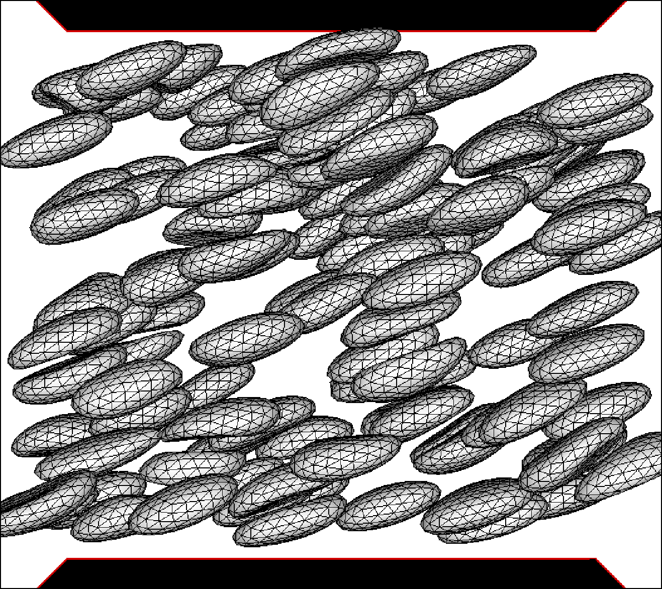
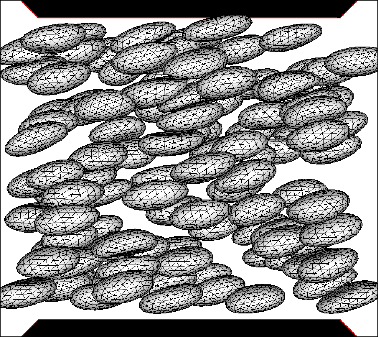


In this section, we report results from several large scale simulations on multiparticle suspensions of capsules. In the first part of the section, we present results for the suspension viscosity and discuss its dependence on the viscosity ratio. In the second part, we discuss the expected computational complexity of the algorithm and verify it with timing results from the multiparticle simulations.
7.1 Suspension viscosity
We consider here a suspension of Neo-Hookean capsules in a cubic slit (Fig. 13a,b). These suspensions are subjected to a simple shear flow at a capillary number of ; the volume fraction of the suspension is , which is typical of the blood flow in the microcirculation [17]. Capsules with five different viscosity ratios are considered: , 2, 3, 4, and 5. The surface of each of the capsules was discretized into triangular elements, while four different system sizes were considered with the number of particles being , , , and . In each of the problems, was kept fixed, where is radius of the spherical capsule at rest. Similar to Sec. (6.4), the capsules were preinflated by to prevent membrane buckling; the radius after preinflation is denoted by . The number of mesh points for the global solution varied between and such that in all cases with . For testing the convergence of the results with respect to GGEM parameters, some simulations were also run with extra mesh points in each of the directions corresponding to . We discuss next an important issue in multiparticle simulations, which concerns the treatment of near singular integrals – these integrals arise when the gaps between the particles become small.
In a suspension of particles subjected to shear, it is not uncommon to find particle pairs separated by a small gap. This is true, at least occasionally, even in suspensions with a moderate volume fraction such as studied here. When the gap between a particle pair becomes small, the interparticle contributions between such a pair from both the single as well as the double layer integrals become nearly singular; these nearly singular integrals require special treatment or the simulations may diverge [65]. In the literature, several techniques have been proposed to address this numerically difficult problem. A few among these are the near singularity subtraction technique [43, 65] and coordinate mapping techniques [47] for the evaluation of the near singular integrals. These techniques will, however, require very high surface mesh resolution and very high order quadrature techniques for the accurate evaluation of the nearly singular integrals [16, 62] – the cost associated with these requirements can be prohibitive. An alternative approach is the use of a short range repulsive force, which can prevent the formation of small gaps [16], though this is not very effective in three dimensional simulations [63]. The best approach appears to be an overlap correction in an auxiliary step [63]. This approach is also frequently used in suspensions of rigid particles [15, 45, 32]. In the present work, like in past efforts [45, 63], we not only correct the overlaps, but also maintain a minimum gap () between the surfaces of two particles. This approach was also employed in our recent work [31]. For simulations in the current section, we set the minimum gap parameter to a small value of .
The overlap correction procedure employed in this work involves moving a pair of overlapping particles apart along their line of centers like a rigid particle until the minimum gap requirement is satisfied. Translating the capsules like a rigid particle in this auxiliary step has the benefit that the shapes of the particles remain unchanged, as is the orientation of the particles with respect to the flow. In general, multiple steps of the correction procedure is required, as the correction of overlap between one pair could result in other overlaps [15, 45]. This overlap correction step involves minimal displacement of the particles, on the order of . Given that the volume fraction studied in this work is , this procedure was rarely required – on an average, less than particle pairs in the particle system exhibited minimum gap violations at any given time. We finally remark that apart from correcting the minimum gap violations in the system, no special treatment was accorded to the evaluation of the near singular integrals in the present effort.
Having discussed the procedure for controlling the minimum gap in the system, we now turn to the results from multiparticle simulations. All these simulations were initiated by placing the particles randomly in the simulation box, and then they were sheared for a total non-dimensional time of . We show some representative snapshots from particle simulations in Figs. (13a) and (13b) for and capsules, respectively. It is immediately obvious from these snapshots that the more viscous capsules deform less and also have a smaller inclination angle with the flow direction; both of these observations are similar to observations in isolated sheared capsules [54]. The convergence of the simulation with respect to GGEM parameters is demonstrated in Fig. (13c), where we plot the suspension apparent intrinsic viscosity for capsule and particle system for two different mesh resolutions corresponding to and . The apparent intrinsic viscosity is defined as , where is the particle contribution to shear stress, while is the suspending fluid viscosity. The particle contribution to the stress tensor is given by [29]
| (65) |
where the sum in the right hand side is over all the particles in the system. As can be seen in Fig. (13c), is nearly identical for simulations run with and , thereby demonstrating the convergence of the simulation with respect to GGEM parameters. All the remaining simulations were performed with . The effect of viscosity ratio on the apparent intrinsic viscosity is shown in Fig. (13d). These results represent an average over the last time units in the particle systems, which have a confinement ratio of . For a direct comparison, the plot also shows for a dilute suspension of capsules obtained from single particle simulations in the same geometry. In dilute suspensions, a non-monotonic variation of the viscosity with is obvious – this behavior has been demonstrated before in the literature [2]. However, the non-monotonicity vanishes at the non-dilute volume fraction of . This indicates that the contribution to the overall stress from particle-particle interactions is a monotonically increasing function of , and, in non-dilute suspensions, easily compensates the non-monotonic variation of the isolated particle contribution. Hence caution is warranted before extrapolating trends from dilute systems to non-dilute systems like blood flow.
7.2 Computational complexity
We devote the remainder of this section to analyzing the overall computational complexity of our algorithm. Before presenting the timing results from the detailed numerical simulations presented above, it will be useful to first discuss the expected computational cost associated with various steps in the algorithm, and consequently the overall implementation. The first step in the solution procedure, as discussed in Sec. (5), involves iteratively solving for the single layer density (step 1). This is followed by the computation of the fluid velocity at the element nodes (step 2) using the single layer density computed in the previous step. The computational cost associated with each iteration of step 1 and that of step 2 has an identical optimal scaling with , each of which is essentially determined by the computational cost associated with the Stokes flow solver (GGEM) described in Sec (3.2). Therefore, for a direct cost comparison with the multiparticle flow problem here, we consider an auxiliary problem involving a collection of point forces; both problems then have an identical computational cost scaling with . At this stage, it will also be worth pointing out that the computational complexity analysis presented here closely follows the corresponding analysis in PME like methods [40, 41] as the underlying ideas are fairly similar.
The overall cost associated with the GGEM Stokes flow solver is the sum of costs associated with the local problem and the global problem. The cost of the local solution scales as the product of the number of point forces and the number of neighbors within a distance of each of the point forces. If we require the computational cost of the local problem to scale as , then the number of neighbors per point force must stay constant with changing system size (meaning here). The system size can be increased in two contrasting ways: (i) by increasing volume at constant density (i.e., by increasing while maintaining constant, is the system volume), and (ii) by increasing density at constant volume (i.e., by increasing while maintaining constant). If the system size is increased at constant density, we require that (or ) be held constant, and if the system size is increased at constant volume, we require that (or ). This scheme for choosing ensures that the average number of near neighbors per point force is independent of the system size. Hence, irrespective of how is varied, we always obtain . Next, we determine the computational cost of the global solution procedure. Before we proceed further, it is important to realize that the error in the global solution is essentially controlled by the parameter 11 1 the error in the local solution is set by the choice of the parameter , which is unchanged with changing ; see Sec. (3.2.2). Therefore, for the error in the global solution to remain of the same order with changing system size , we require that be held constant; this implies . Coupling this requirement with the choices of discussed above in different scenarios, we conclude that the total number of mesh points involved in the calculation of the global solution must be varied proportionally to , i.e. . Having determined the scaling of , we next present the expression for the computational cost of the global solution as follows:
| (66) |
where the first two terms on the right hand side denote the cost associated with the FFT operations in and directions respectively, while the last term is associated with the cost of the Chebyshev-tau solver in the wall normal direction. Note that the cost in the expression for the Chebyshev-tau solver is associated with the quasi-tridiagonal solve, while cost is associated with the computation of the Chebyshev transforms and its inverse with FFTs. Simplifying the above expression and noting that , we obtain the following asymptotic scaling
| (67) |
The overall cost per iteration of step 1 or of step 2 is therefore,
| (68) |
The total cost of step 1 is the cost per iteration times the number of iterations required for convergence. Now, if the number of iterations in step 1 is independent of , then the computational cost of the overall algorithm will scale as . On the other hand, if the number of iterations in step 1 is dependent on the system size, say it scales as , then the computational cost of the overall algorithm will scale as:
| (69) |
Note that the need for iterative solution of step 1 or a related second kind integral equation is not unique to the present formulation, but is a general feature of any accelerated boundary integral method with [63].

Having determined the expected scaling of our algorithm, we next report timing results from the detailed numerical simulations presented in Sec. (7.1). All runs were performed on a single core of a eight core machine with a 2 GHz Intel Xeon processor running Linux. We plot the time required per stage of the two stage midpoint time stepping algorithm in Fig. (14). Note that the abscissa in the plot is ; the four data points in this plot are respectively for , , and as discussed above. One can conclude from this plot that in all cases the computational cost scales approximately as (in fact, in this case, the increase in the computational cost appears to be slower than the expected ). Another important feature to note in the plot is the jump in computational cost as one moves from a matched viscosity problem to a non-matched one, which is expected as no iterations are required in matched viscosity problems. The number of iterations required for convergence was found to be independent of the system size for problems considered here, though it was found to increase with increasing . The simulations with capsules required approximately 2 iterations on an average, while the simulations with capsules required approximately 3 iterations. To summarize this section, we note that a near perfect scaling of is obtained for both matched viscosity and non-matched viscosity problems. A few words of caution are necessary here, though, as at higher volume fractions and/or at much larger system sizes, the number of iterations for convergence is expected to become system size dependent. It must be emphasized here that this aspect is not specific to our implementation, but is intrinsic to the boundary integral equation for non-matched viscosity problems. Future work on enhancements in the algorithm should address this by the development of efficient preconditioners. Another obvious enhancement in the algorithm will be its parallelization to take advantage of cheaply available multicore processors.
8 Conclusions
A new accelerated boundary integral method for multiphase Stokes flow in a confined geometry was presented. The complexity of the method scales as for the slit geometry discussed in the present paper. The acceleration in the method was provided by the use of General Geometry Ewald-like (GGEM) method for the fast computation of the velocity and stress fields driven by a set of point forces in the geometry of interest. Due to non-periodic nature of the domain, an alternative boundary integral formulation was employed, necessitated by the requirements of the acceleration technique. An efficient methodology was presented to compute the resulting double and single layer integrals using the GGEM technique. The resulting implementation was validated with several test problems. The computational complexity of the algorithm was verified to be with timing results from several large scale multiparticle simulations.
Acknowledgments
The authors gratefully acknowledge helpful discussions with Pratik Pranay, Yu Zhang and Juan Hernandez-Ortiz on the implementation of GGEM. This work was supported by NSF Grants CBET-0852976 and CBET-1132579.

Appendix A Derivation of Boundary Integral equation
Consider a two phase flow in a specified geometry as shown in Fig. (1). The two fluids are respectively denoted by and in the figure with viscosity and . The fluid is assumed to be enclosed by an impermeable interface denoted by , which has its own characteristic properties (e.g. drops, capsules, vesicles, etc). Now, consider a point in fluid as shown in Fig. (15). Applying the reciprocal theorem to the disturbance velocity in the region denoted by , and that due to a point force located at , we obtain
| (70) |
where is the hydrodynamic traction at the interface on the side of fluid associated with the velocity field , while is the Green’s function for the specified geometry and is the associated stress tensor. Next, employing the self-adjointness property of the Green’s function , we obtain the following form of the above equation
| (71) |
Recall that the self-adjointness of the Green’s function implies that
| (72) |
Next, we apply the reciprocal theorem to the undisturbed flow in region and due to a point force located at in region . This yields,
| (73) |
Note that in the above equation, the normal is pointing out of region into region (outward normal). We next note the following relation between and
| (74) |
This follows from the continuity of the undisturbed flow across the interface, and that the internal and external stresses are computed with viscosity and respectively for the same flow field. Using this relationship, we write Eq. (73) as
| (75) |
Adding Eqs. (71) and (75), we obtain
| (76) |
Next, we apply reciprocal theorem to the fluid velocity in region 2 () and due to a point force located at . This yields
| (77) |
For interfacial flows neither the interfacial velocity nor the interface tractions on either side is known, though we have the following boundary conditions at any point on the interface
| (78a) |
| (78b) |
which essentially implies the continuity of the velocity across the interface and that the net force on an element due to hydrodynamic stresses is balanced by the net force due to interfacial stresses, see Sec. (4). We note that the interfacial contribution is assumed to be known by the known constitutive equation of the interface and its known configuration. Given the unknowns and the boundary conditions, a very common approach is to eliminate the unknown hydrodynamic interfacial tractions and with the known traction jump in Eqs. (76) and (77). This leads to the widely employed second kind integral equation for the unknown interfacial velocity. Here, we adopt an alternative approach. Using Eqs (76) and (77) we instead eliminate the double layer integral to obtain
| (79) |
The above can be written in the following form
| (80) |
This equation for the velocity can be shown to be valid inside, outside, as well as on the boundary . The drawback of this equation is that both the velocity (including interfacial velocity) and the surface tractions are unknown. The main advantage for our purposes here is that we have switched the pole and the field point of the Green’s function using its self-adjointness property (Eq. 72). For simplifying the notation, we next express the operand of the Green’s function by , i.e. we define as
| (81) |
Using the above definition, we write the velocity as
| (82) |
The pressure associated with the above velocity field in the region external to can be written as
| (83) |
Using Eqs. (82) and (83), we can write the stress as
| (84) |
A similar expression can be written for as shown below:
| (85) |
We will now take the limit of the above equations as we approach the interface from either side and then dot it with the normal to get the tractions on either side of the interface and . We can express both of them using the principal value of the double layer integral along with the jump condition to obtain [50]
| (86a) |
| (86b) |
where implies the principal value of the improper integral when the observation point lies on the domain of the integration. Note that the sign of the jump condition () depends on the direction from which we approach the interface relative to the outward normal defined above, i.e. whether we approach the interface parallel to the normal or anti to it.
Taking the difference of Eqs. (86a) from (86b) and using Eqs. (78b) and (74), we have that
| (87) |
where we have now introduced the viscosity ratio . Rearranging the above equation, we obtain a second kind integral equation for the density of the Green’s function as follows:
| (88) |
where we have defined as
| (89) |
The above equation is used to solve for the unknown density , which upon substitution in Eq. (82) gives the velocity at any point in the domain, including the interface.
Appendix B Undisturbed flow stress
For pressure driven flows, the stress tensor is given by
| (90) |
where is
| (91) |
Note that the velocity and pressure field in pressure driven flows is given by the following expressions
| (92a) |
| (92b) |
In the above equations, is the centerline velocity. The surface traction can be obtained at a point on the surface with normal vector as
| (93) |
For simple shear flows, the stress tensor is given by
| (94) |
where is the shear rate. The surface traction for this case can be obtained by substituting the stress tensor in the above equation in Eq. (93).
Appendix C Fast Spectral Stokes Flow Solver
Here we discuss the solution procedure for the global problem in Eq. (3.2) for a slit geometry (Fig. 1). We simplify the notation in Eq. (3.2) and represent it by the following set of equations:
| (95a) |
| (95b) |
where is the pressure, is the velocity, while is a known function obtained from the known distribution of global force densities. The above set of equations are supplemented by the periodic boundary conditions in and directions, while a Dirichlet boundary condition for the velocity is specified in the y direction:
| (96a) |
| (96b) |
The velocity and pressure variables are first expanded in truncated Fourier series in and directions as:
| (97) |
Similar expressions are written for , , , , , and by replacing by , , , , , and respectively in the above equation. Substituting this in equation (C) and employing the Galerkin method, we obtain the following owing to the orthogonality of Fourier modes:
| (98a) |
| (98b) |
| (98c) |
| (98d) |
where we have dropped the subscript in the above equation. Next, using the last equation, we eliminate , and in the first three equations to obtain the following equation for the pressure:
| (99) |
The continuity equation can be replaced by the above equation for pressure along with the boundary condition requiring the velocity to be divergence free [10, 7], i.e.
| (100) |
Alternatively, one solves the Eq. 99 with the following pressure boundary condition
| (101a) |
| (101b) |
though, the pressure boundary conditions above are unknown a priori, but instead they must take a value so that the condition in Eq. (100) is satisfied. Grouping all the equations to be solved, we have the following
| (102a) |
| (102b) |
| (102c) |
| (102d) |
with the following boundary conditions
| (103) |
where and and, as with the other quantities, denotes discrete Fourier transform in and .
The Kleiser-Schumann influence matrix approach involves solving three set of equations as in Eq. (C) with different boundary conditions as discussed shortly. In the first set, one solves the equations in C with the correct boundary conditions for the velocity in Eq. (103), but with homogeneous boundary conditions for the pressure, i.e.
| (104) |
Each of the equations for pressure and velocity components above are solved here by expanding them in discrete Chebyshev polynomials and then employing the Galerkin method to obtain equations for each of Chebyshev modes. The appropriate boundary conditions are satisfied by employing the tau method [6, 49] in which the equations for the highest two Chebyshev modes are replaced by the boundary condition equations. The solution for pressure is first computed, whose value is then substituted in the equations for velocity. Thus, in each step, one needs to solve a Helmholtz equation using Chebyshev polynomial expansion. In this case, the equations for the unknown Chebyshev coefficients can be reduced to a quasi-tridiagonal matrix equation with the last full row being full, while the rest being in the standard tridiagonal form. Also, note that the equations for the even and odd Chebyshev modes are decoupled and solved separately. These quasi-tridiagonal systems of equations can be solved in time with a direct algorithm [49]. Also, the use of Chebyshev Gauss-Lobatto quadrature points [6, 49] for transforming a variable between physical and transform space ensures that FFTs can be employed for its evaluation [7]. Therefore, for each of the Fourier modes , the asymptotic cost of the Chebyshev-tau solution procedure scales as . We denote this first set of solution thus obtained for Fourier mode by ().
The next two sets of equations involve solving the homogeneous version of the differential equations in C, i.e., the right hand side of the each of the equations in C is set to zero. Moreover, the velocity boundary condition for these two sets of problems are also homogeneous. The only non-homogeneous equation in these two problems are the pressure boundary conditions. In the first of these, the pressure boundary condition is the following:
| (105) |
while in the second the pressure boundary condition is
| (106) |
We denote these two solutions by (), and (). It is important to note that the latter two set of equations are to be solved just once at the beginning of the simulation and the results are stored. The overall solution for the velocity and pressure is then obtained as:
| (107) |
It is easy to see that the above solution satisfies both the differential equations as well as the boundary conditions. The only remaining task is therefore to determine the pressure boundary conditions and . This is accomplished by the requiring that the velocity be divergence free at the boundary (Eq. 100). Thus, one obtains the following equations for the pressure boundary conditions
| (108) |
In the above equations, , and are the continuity expression (Eq. 100) evaluated at the appropriate boundary point, i.e. at or . For example, is given by
| (109) |
The coefficient matrix in Eq. (108) is known as the influence matrix and the resulting matrix equation is trivially solved at a cost of . The solution in Eq. (107) gives the Fourier coefficients of the pressure and velocity as a function of the wall normal coordinate , which is then employed to obtain the pressure and velocity in the physical space using inverse FFTs.
References
- [1] Allen, M. P., Tildesley, D. J., 1989. Computer Simulation of Liquids. Oxford University Press.
- [2] Bagchi, P., Kalluri, R. M., 2010. Rheology of a dilute suspension of liquid-filled elastic capsules. Physical Review E 81, 056320.
- [3] Barthes-Biesel, D., 2011. Modeling the motion of capsules in flow. Current Opinion in Colloid & Interface Science. 16, 3–12.
- [4] Barthes-Biesel, D., Diaz, A., Dhenin, E., 2002. Effect of constitutive laws for two-dimensional membranes on flow-induced capsule deformation. Journal Of Fluid Mechanics 460, 211–222.
- [5] Blake, J. R., 1971. A note on the image system for a stokeslet in a no-slip boundary. Proceedings of the Cambridge Philosophical Society 70, 303–310.
- [6] Canuto, C., Hussaini, M. Y., Quarteroni, A., Zang, T. A., 2006. Spectral Methods Fundamentals in Single Domain. Springer-Verlag.
- [7] Canuto, C., Hussaini, M. Y., Quarteroni, A., Zang, T. A., 2007. Spectral Methods Evolution to Complex Geometries and Applications to Fluid Dynamics. Springer-Verlag.
- [8] Charrier, J. M., Shrivastava, S., Wu, R., 1989. Free and constrained inflation of elastic membranes in relation to thermoforming - non-axisymmetric problems. Journal Of Strain Analysis For Engineering Design 24, 55–74.
- [9] Deserno, M., Holm, C., 1998. How to mesh up ewald sums. i. a theoretical and numerical comparison of various particle mesh routines. Journal of Chemical Physics 109, 7678–7693.
- [10] Deville, M., Kleiser, L., Montigny-Rannou, F., 1984. Pressure and time treatment for chebyshev spectral solution of a stokes problem. International Journal for Numerical Methods in Fluids 4, 1149–1163.
- [11] Doddi, S. K., Bagchi, P., 2009. Three-dimensional computational modeling of multiple deformable cells flowing in microvessels. Physical Review E 79, 046318.
- [12] Elman, H. C., Silvester, D. J., Wathen, A. J., 2005. Finite elements and fast iterative solvers: with applications in incompressible fluid dynamics. Oxford University Press.
- [13] Fard, A. S., Hulsen, M., Meijer, H., Famili, N., Anderson, P., 2012. Adaptive non-conformal mesh refinement and extended finite element method for viscous flow inside complex moving geometries. International Journal for Numerical Methods in Fluids 68 (8), 1031–1052.
- [14] Ferziger, J. H., Peric, M., 2002. Computational methods for fluid dynamics. Springer-Verlag.
- [15] Foss, D. R., Brady, J. F., 2000. Brownian Dynamics simulation of hard-sphere colloidal dispersions. Journal of Rheology 44, 629–651.
- [16] Freund, J. B., 2007. Leukocyte margination in a model microvessel. Physics of Fluids 19, 023301.
- [17] Fung, Y. C., 1996. Biomechanics: Circulation, 2nd Edition. Springer-Verlag.
- [18] Greengard, L., Kropinski, M. C., Mayo, A., 1996. Integral equation methods for stokes flow and isotropic elasticity in the plane. Journal of Computational Physics 125, 403–414.
- [19] Greengard, L., Lee, J.-Y., 2004. Accelerating the nonuniform fast fourier transform. SIAM Review 46, 443–454.
- [20] Greengard, L., Rokhlin, V., 1987. A fast algorithm for particle simulations. Journal of Computational Physics 73, 325–348.
- [21] Griggs, A. J., Zinchenko, A. Z., Davis, R. H., 2007. Low-Reynolds-number motion of a deformable drop between two parallel plane walls. International Journal of Multiphase Flow 33, 182–206.
- [22] Hasimoto, H., 1959. On the periodic fundamental solutions of the Stokes equations and their application to viscous flow past a cubic array of spheres. Journal of Fluid Mechanics 5, 317–328.
- [23] Henniger, R., Obrist, D., Kleiser, L., 2010. High-order accurate solution of the incompressible Navier-Stokes equations on massively parallel computers. Journal of Computational Physics 229, 3543–3572.
- [24] Hernandez-Ortiz, J. P., de Pablo, J. J., Graham, M. D., 2007. Fast computation of many-particle hydrodynamic and electrostatic interactions in a confined geometry. Physical Review Letters 98, 140602.
- [25] Hernandez-Ortiz, J. P., Ma, H., de Pablo, J. J., Graham, M. D., 2008. Concentration distributions during flow of confined flowing polymer solutions at finite concentration: slit and grooved channel. Korea-Australia Rheology Journal 20, 143–152.
- [26] Hughes, T. J. R., 1987. The Finite element method : linear static and dynamic finite element analysis. Prentice-Hall.
- [27] Janssen, P. J. A., Anderson, P. D., 2007. Boundary-integral method for drop deformation between parallel plates. Physics of Fluids 19, 043602.
- [28] Janssen, P. J. A., Anderson, P. D., 2008. A boundary-integral model for drop deformation between two parallel plates with non-unit viscosity ratio drops. Journal of Computational Physics 227, 8807–8819.
- [29] Kennedy, M. R., Pozrikidis, C., Skalak, R., 1994. Motion and deformation of liquid drops, and the rheology of dilute emulsions in simple shear flow. Computers & Fluids 23, 251–278.
- [30] Kim, S., Karrila, S. J., 2005. Microhydrodynamics: Principles and Selected Applications. Dover Publicatons.
- [31] Kumar, A., Graham, M. D., 2011. Segregation by membrane rigidity in flowing binary suspensions of elastic capsules. Physical Review E 84, 066316.
- [32] Kumar, A., Higdon, J. J. L., 2010. Origins of the anomalous stress behavior in charged colloidal suspensions under shear. Physical Review E 82, 051401.
- [33] Kumar, A., Higdon, J. J. L., 2011a. Dynamics of the orientation behavior and its connection with rheology in sheared non-brownian suspensions of anisotropic dicolloidal particles. Journal of Rheology 55, 581–626.
- [34] Kumar, A., Higdon, J. J. L., 2011b. Particle mesh ewald stokesian dynamics simulations for suspensions of non-spherical particles. Journal of Fluid Mechanics 675, 297–335.
- [35] Lac, E., Barthés-Biesel, D., Pelekasis, N. A., Tsamopoulos, J., 2004. Spherical capsules in three-dimensional unbounded Stokes flows: effect of the membrane constitutive law and onset of buckling. Journal of Fluid Mechanics 516, 303–334.
- [36] Lac, E., Morel, A., Barthès-Biesel, D., 2007. Hydrodynamic interaction between two identical capsules in simple shear flow. Journal of Fluid Mechanics 573, 149–169.
- [37] Lambert, J. D., 1997. Numerical Methods for Ordinary Differential Systems: The Initial Value Problem. John Wiley & Sons Ltd.
- [38] Le, D.-V., Tan, Z., 2010. Large deformation of liquid capsules enclosed by thin shells immersed in the fluid. Journal of Computational Physics 229, 4097–4116.
- [39] Li, X., Sarkar, K., 2008. Front tracking simulation of deformation and buckling instability of a liquid capsule enclosed by an elastic membrane. Journal of Computational Physics 227, 4998–5018.
- [40] Lindbo, D., Tornberg, A.-K., 2010. Spectrally accurate fast summation for periodic stokes potentials. Journal of Computational Physics 229, 8994–9010.
- [41] Lindbo, D., Tornberg, A.-K., 2011. Spectral accuracy in fast ewald-based methods for particle simulations. Journal of Computational Physics 230, 8744–8761.
- [42] Liron, N., Mochon, S., 1976. Stokes flow for a stokeslet between two parallel flat plates. Journal of Engineering Mathematics 10, 287–303.
- [43] Loewenberg, M., Hinch, E. J., 1996. Numerical simulation of a concentrated emulsion in shear flow. Journal of Fluid Mechanics 321, 395–419.
- [44] MacMeccan, R. M., Clausen, J. R., Neitzel, G. P., Aidun, C. K., 2009. Simulating deformable particle suspensions using a coupled lattice-Boltzmann and finite-element method. Journal of Fluid Mechanics 618, 13–39.
- [45] Meng, Q., Higdon, J. J. L., 2008. Large scale dynamic simulation of plate-like particle suspensions. part ii: Brownian simulation. Journal of Rheology 52, 37–65.
- [46] Metsi, E., 2000. Large scale simulation of bidisperse emulsions and foams. Ph.D. thesis, University of Illinois at Urbana-Champaign.
- [47] Muldowney, G., Higdon, J. J. L., 1995. A spectral boundary element approach to three-dimensional Stokes flow. Journal of Fluid Mechanics 298, 167–192.
- [48] Noguchi, H., Gompper, G., 2005. Shape transitions of fluid vesicles and red blood cells in capillary flows. Proceedings of the National Academy of Sciences, USA 102, 14159–14164.
- [49] Peyret, R., 2002. Spectral Methods for Incompressible Viscous Flow. Springer-Verlag.
- [50] Pozrikidis, C., 1992. Boundary Integral and Singularity Methods for Linearized Viscous Flow. Cambridge University Press.
- [51] Pranay, P., Anekal, S. G., Hernandez-Ortiz, J. P., Graham, M. D., 2010. Pair collisions of fluid-filled elastic capsules in shear flow: effects of membrane properties and polymer additives. Physics of Fluids 22, 123103.
- [52] Rahimian, A., Veerapaneni, S. K., Biros, G., 2010. Dynamic simulation of locally inextensible vesicles suspended in an arbitrary two-dimensional domain, a boundary integral method. Journal of Computational Physics 229, 6466–6484.
- [53] Rallison, J. M., 1981. A numerical study of the deformation and burst of a viscous drop in general shear flows. Journal of Fluid Mechanics 109, 465–482.
- [54] Ramanujan, S., Pozrikidis, C., 1998. Deformation of liquid capsules enclosed by elastic membranes in simple shear flow: large deformations and the effect of fluid viscosities. Journal of Fluid Mechanics 361, 117–143.
- [55] Saad, Y., 2003. Iterative Methods for Sparse Linear Systems. Society for Industrial and Applied Mathematics.
- [56] Silvester, D. J., Wathen, A. J., 1994. Fast iterative solution of stabilised Stokes systems part ii: Using general block preconditioners. SIAM Journal on Numerical Analysis 31, 1352–1367.
- [57] Smart, J. R., Leighton, D. T., 1991. Measurement of the drift of a droplet due to the presence of a plane. Physics of Fluids A 3, 21–28.
- [58] Staben, M. E., Zinchenko, A. Z., Davis, R. H., 2003. Motion of a particle between two parallel plane walls in low-reynolds-number Poiseuille flow. Physics of Fluids 15, 1711–1733.
- [59] Stone, H. A., Stroock, A. D., Ajdari, A., 2004. Engineering flows in small devices: Microfluidics toward a lab-on-a-chip. Annual Review of Fluid Mechanics 36, 381–411.
- [60] Swan, J. W., Brady, J. F., 2011. The hydrodynamics of confined dispersions. Journal of Fluid Mechanics 687, 254–299.
- [61] Thibault, J. C., Senocak, I., 2009. Cuda implementation of a Navier-Stokes solver on multi-gpu desktop platforms for incompressible flows. In: 47th AIAA Aerospace Sciences Meeting.
- [62] Veerapaneni, S. K., Rahimian, A., Biros, G., Zorin, D., 2011. A fast algorithm for simulating vesicle flows in three dimensions. Journal of Computational Physics 230, 5610–5634.
- [63] Zhao, H., Isfahani, A. H. G., Olson, L. N., Freund, J. B., 2010. A spectral boundary integral method for flowing blood cells. Journal of Computational Physics 229, 3726–3744.
- [64] Zinchenko, A. Z., Davis, R. H., 2000. An efficient algorithm for hydrodynamical interaction of many deformable drops. Journal of Computational Physics 157, 539–587.
- [65] Zinchenko, A. Z., Davis, R. H., 2002. Shear flow of highly concentrated emulsions of deformable drops by numerical simulations. Journal of Fluid Mechanics 455, 21–62.