Rapid Accurate Calculation of the $s$-wave Scattering Length

We begin by introducing a mapping function $y=y(r)$ that is a smooth, monotonically increasing function of the radial coordinate $r$ and maps $[0,\infty)$ onto the finite domain $[a,b]$. The well-known substitution [18, 17]

then transforms the conventional radial Schrödinger equation (2) into the equivalent form

in which

whose additive term is defined as

Hereafter, a prime (^′) symbol denotes differentiation with respect to our new radial variable $y$.

It should be noted that:

1. 1.

   the modified wave function $\phi(y)$ is now defined on the finite domain $[a,b]$;

2. 2.

   the modified radial equation (7) is completely equivalent to the initial one (2), as long as $r(y)\in(\mathcal{C}^{3}[a,b])$ is a monotonically increasing function;

3. 3.

   a knowledge of the inverse analytical function $r(y)$ is all that is required to accomplish the exact transformations of Eqs. (6)-(9);

4. 4.

   for a fixed mesh of equally spaced $y$ points on the interval $y\in[a,b]$, the function $\rho(r)=dy/dr=1/g(y)$ defines the density distribution of mesh points of the initial coordinate $r$.

It is clear that conventional finite-difference [23, 24, 26, 21] and pseudospectral [22] methods can be used straightforwardly for integrating the transformed radial equation (7) out to the point $y=b$, as long as the modified wave function $\phi(y)$ is not singular anywhere on the interval $[a,b]$, and especially not at its end points. Furthermore, it will be proved in the next section that the scattering length $a_{s}$ is an explicit function of logarithmic derivative of the wave function $\phi(y)$

at the boundary $y=b$. It is well-known that the transformation (10) converts the radial equation (7) into the modified Ricatti equation

which can be numerically integrated, for instance, using Johnson’s efficient log-derivative method [23, 24]. More details regarding this method are given in the Appendix.

Since Eq. (4) shows that the scattering length can be expressed formally in terms of the asymptotic behavior of the ordinary radial wavefunction $\psi(r)$, we can write

It therefore seems desirable to investigate the asymptotic behavior of the modified function $\phi(y)$ near the outer boundary point $y=b$ corresponding to $r\to\infty$, where

Since we are mapping an infinite interval onto a finite one, it is clear that the mapping function $r(y)$ must have a singularity at the upper end of the interval. To proceed, we assume that this singularity has the form

where necessarily $\gamma>0$, because the $r(y)$ function must go to infinity as $y$ approaches $b$ in order to convert the finite domain $y\in[a,b]$ into the infinite one $r\in[r_{\rm min},+\infty]$.

Inserting Eq. (14) into Eq. (13) yields

and differentiating that result with respect to $y$ yields

From Eqs.(15) and (16) it is immediately clear that for both the modified wave function $\phi(y)$ and its derivative $\phi^{\prime}(y)$ to be non-singular at the point $y=b$ (or $r=+\infty$), necessarily $\gamma=1$.

Avoidance of this singularity at $y=b$ is clearly desirable if we are to integrate the modified radial equation (7) accurately on the whole interval $[a,b]$, so it is necessary to choose a mapping function $r(y)$ that has only a simple pole at the end point $y=b$. Let us assume that $r(y)$ can be expressed as a Laurent series expansion about this point:

where $\,c_{-1}>0$. Inserting Eq. (17) into Eq. (13) and differentiating the resulting expression for $\phi(y)$ with respect to $y$ yields, at the point $y=b$,

which shows that

is the desired relationship between the scattering length $a_{s}$ and the log-derivative function at the outer end of the interval, $\xi(b)$.

To facilitate accurate calculation of the the required $\xi(b)$ value, it is desirable that the function $\widetilde{Q}(y)$ of Eq. (8) be nonsingular at the end point $y=b$. It is easy to verify that the $F(y)$ contribution is nonsingular at $y=b$, since

Moreover, from Eq. (17) it is clear that in the limit $\,y\to b\,$ (or $\,r\to\infty$),

This means that for any potential which dies off more slowly than $1/r^{4}$, the product $g^{2}\,U(r)$ that comprises the main part of the function $\widetilde{Q}(y)$ (see Eq. (8)) diverges in the limit $y\to b$ $(r\to+\infty)$. In particular, if $\,U(r\to\infty)\simeq-\,C_{n}/r^{n}\,$, then as $\,y\to b\,$,

and hence

This means that, to calculate the modified wavefunction $\phi(y)$ and/or its derivative $\phi^{\prime}(y)$ at the end of the range ($y=b$) for an $n=4$ case requires explicit knowledge of the leading long-range induction coefficient $C_{4}$, while for the more common $n=5$ or 6 cases it requires only a knowledge of the mapping function $r(y)$ that defined $F(b)$. In contrast, for $\,n<4\,$ no satisfactory determination of $\phi(b)$ and/or $\phi^{\prime}(b)$ can be achieved using the present approach. This latter result is consonant with the fact that the scattering length is not defined for potentials that die off more slowly than $1/r^{4}$ [1].

To make practical use of our relationship (19) between the scattering length and the log-derivative function, it is necessary to introduce an analytical mapping function with the Laurent expansion form of Eq. (17). The simplest way to do this is to define the mapping function as the first two terms of the Laurent series:

since only the $c_{-1}$ and $c_{0}$ coefficients are required in Eq. (19). In particular, setting $b=1$ and $\,c_{-1}/2=-c_{0}\equiv\bar{r},$ in (27) yields a version of (omitting a factor of 2) of the well-known Ogilvie-Tipping (OT) potential energy expansion variable [19]:

For this case Eq. (19) shows that the scattering length is explicitly defined as

while the reciprocal mapping function is

and

Moreover, for this mapping function the additive term $F_{\texttt{OT}}(y)=0$.

Use of the simple one-parameter mapping function of Eq. (28) does provide a reliable method for calculating $a_{s}$. However, our recent experience with applying this type of transformation to bound-state problems [18] suggests that better efficiency may be attained using more flexible two-parameter functions. One such function which was successfully used for bound-state calculations is the two-parameters ($\bar{r}$, $\alpha>0$) Šurkus variable [20]:

for which the reciprocal mapping function is

However, except for the special case $\alpha=1$ in which $y_{\rm S}(r;\bar{r},\alpha)$ reduces to $y_{\texttt{OT}}(r;\bar{r})$, this mapping function is not appropriate for scattering-length calculations, since when $\alpha\neq 1$ the mapping function $r_{\rm S}(y)$ does not take on the required Laurent series expansion form (17) as $y\to 1$, so the associated log-derivative wavefunction $\xi(y)$ becomes singular there.

In contrast, the two-parameters tangential function [22]

defined on the interval $y\in[(2/\pi)\tan^{-1}(-\beta),1]$, whose inverse is the inverse tangent function

completely conforms to the required Laurent expansion form of Eg. (17) as $y\to 1$, since

For this case

and it is easy to show that the additive contribution to Eq. (8) is a constant,

and that

The optimal values of the parameters defining the mapping function of Eq. (34) may be expected to depend both on the nature of the interaction potential $U(r)$ and on the particular numerical method used for integration of the modified radial equation (7). When using Johnson’s log-derivative method of integration [23, 24], the optimal mapping parameters $\bar{r}$ and $\beta$ could be determined by minimizing the truncation error $\Delta\xi$ estimated using a Richardson extrapolation (RE) (66), or by minimizing the difference between $\xi_{h_{1}}(y=b)$ and $\xi_{h_{2}}(y=b)$ values corresponding to two different integration step sizes $h_{1}$ and $h_{2}$,

Note that it is tacitly assumed that the optimal parameter values do not depend on the integration step size. This has been confirmed by the illustrative calculations presented in Section III. It will also be shown there that the minimum of the functional (40) is a rather smooth function of both mapping parameters, $\bar{r}$ and $\beta$.

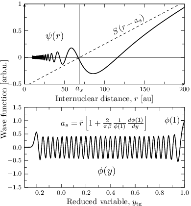
It seems reasonable to assume that the optimal mapping function would correspond to the situation in which

since it is well-known that minimal truncation errors arise in particle-in-a-box problems where the potential $U(r)$ does not depend on $r$. Furthermore, within the classically allowed region where $Q\gg 0$, the additive term $F(y)$ can be approximately neglected [1, 16]. In this case Eq. (41) reduces to $g^{2}\,Q\approx const$, and inverting this condition (recalling that $g(y)\equiv dr/dy$) yields

Here $r_{0}$ is the left-hand (inner) classical turning point, which is the root of the equation $U(r_{0})=0$.

Differentiating Eq. (42) with respect to $r$ yields

For optimal mapping, therefore, the density function $\rho_{\rm opt}(r)$ should be close to $\sqrt{Q(r)}$ in the $Q(r)\gg 0$ region where the original wavefunction $\psi(r)$ has its maximum oscillation frequency. From Eq. (43) it follows that the optimal mapping does not depend on the reduced mass $\mu$, because it appear in $Q(r)$ simply as a multiplicative factor. It is also easy to see that the mapping function (42) transforms the modified wavefunction $\phi(y)$ into the familiar particle-in-a-box form

which correlates with the conventional WKB approximation [1, 16] in the classically allowed region where $Q(r)>0$. As is shown by Fig. 1, in contrast to the original wavefunction $\psi(r)$, the modified wavefunction $\phi(y)$ has loops of almost constant amplitude and spacing over the potential well, behavior which is qualitatively very similar to that implied by Eq. (44). It is therefore expected that the WKB mapping of Eq. (42) should be close to “optimal” for all numerical methods (such as the finite-difference and collocation methods) that are based on an equidistant grid in the classical region of motion. It should be stressed, however, that the mapping function defined by Eq. (42) cannot itself be applied for scattering length calculations because it does not satisfy the required asymptotic behavior of Eq. (17), and because it becomes imaginary in the classically forbidden region where $r<r_{0}$.

It is easy seen from Eqs. (31) and (39) that the density function $\rho_{\texttt{OT}}(r)$ corresponding to the one-parameter mapping function of Eq. (28) is proportional to $1/[r+\bar{r}]^{2}$, while that for the two-parameters tangent function of Eq. (35) has a Lorentzian form with a maximum at $\bar{r}$. The plots presented in Fig. 2, show that there is good agreement between the $\rho_{\rm WKB}(r)$ and $\rho_{\rm tg}(r)$ density functions over much of the domain of the wavefunction $\psi(r)$. This leads to the conclusion that the optimal value of parameter $\bar{r}_{\rm opt}$ should be close to the equilibrium internuclear distance $r_{e}$ of the potential $U(r)$. Hence, for the two-parameters mapping function (35), it seems reasonably to fix $\bar{r}_{\rm opt}\approx r_{e}$ and to vary only the single parameter $\beta$. Note that the pronounced differences among the density functions for these three cases at small distances is not very important, because the associated wave function $\psi(r)$ dies off exponentially in this region.

In the following, therefore, parameter $\bar{r}$ of the mapping functions $y_{\texttt{OT}}(r;\bar{r})$ of Eq. (28) and $y_{\rm tg}(r;\bar{r},\beta)$ of Eq. (35) is fixed as $\bar{r}=r_{e}$, while the optimum value of $\beta$ of Eq. (35) is determined from a one-dimensional minimization of the functional of Eq. (40).

A computer program based on the adaptive mapping procedure described above has been written and tested [29], both for a variety of model potentials, and on potentials for real systems taken from the literature. All results were obtained on 32 bit processors, mainly using double-precision arithmetic, but with quadruple-precision calculations being used sometimes in order to delineate the impact of accumulated numerical round-off error. This section presents the results of those illustrative applications, together with some general discussion of the method.

The first sample calculations presented here are for the model Lennard-Jones($2n,n$) potentials

defined by the potential function parameters and system reduced mass listed in Table 1. The first three of these LJ($2n,n$) potentials, each supporting 15 bound vibrational levels, are the same models systems considered in our recent application of this adaptive mapping approach to bound-state problems [18]. The last two LJ($12,6$) potentials have much deeper wells and support 100 vibrational levels. They were introduced here to highlight the efficiency of the present method, since the computational effort of scattering-length calculations increases dramatically as $v_{\textrm{max}}$ and the absolute magnitude of $a_{s}$-values increase.

Converged $a_{s}$-values for five model LJ($2n,n$) potentials are presented in the last column of Table 1. As discussed above, the range-mapping parameter was fixed at $\bar{r}=r_{e}=1$[Å] for both $y_{\texttt{OT}}(r)$ and $y_{\rm tg}(r)$ mapping functions. The optimal $\beta_{\rm opt}$ values for the latter case were determined by minimizing the functional of Eq. (40), yielding the results shown in the column four. It is interesting to see that these empirically determined $\beta_{\rm opt}$ values have essentially the same dependence on the inverse-power $n$ governing the long-range behavior of the potential as was the case for the analogous parameter $\alpha$ of the Šurkus-variable mapping (32) used in the bound-state study of Ref. [18].

The log-log plots in Figs, 3 and 4 show how the relative errors in the calculated $a_{s}$ values

depend on the number of mesh points $N$ used in the radial integration. The reference values $a_{s}^{\rm exact}$ were obtained from calculations using quadruple precision arithmetic by increasing $N$ until the full desired level of convergence was achieved. The numerical ‘noise’ on these plots for $\delta\lesssim 10^{-12}$ indicates the precision limits achieved using ordinary double-precision arithmetic, while the dashed lines show how the convergence trend continues when quadruple-precision arithmetic is used.

The three upper curves in Fig. 3 (labeled JLD) display results obtained using Johnson’s log-derivative method, while the three lower curves illustrate the greatly improved convergence achieved when that approach is coupled to the ($N,N/2$) Richardson extrapolation procedure described in the Appendix. These results clearly confirm the prediction of Eq. (64), that Johnson’s log-derivative method (JLD), and that method combined with a Richardson extrapolation to zero step (JLD-RE), demonstrate $N^{-4}$ and $N^{-6}$ convergence rates, respectively. We see that for these 15-level LJ potentials, the JLD-RE($N,N/2$) method allows us to attain 11-12 significant digits in calculated $a_{s}$ values when using only $N\approx 10^{4}$ radial mesh points.

The results displayed in Fig. 4 show that as expected, the computational effort increases significantly for the 100-level LJ($2n,n$) models, especially for the very last case considered in Table 1, for which the scattering length is extremely large: $a_{s}\approx 10^{4}$ [Å]. However, that even for those cases full double-precision converge is achieved with only $N\approx 10^{5}$. Note that for a given number of grid points, use of the simple one-parameter mapping function $y_{\texttt{OT}}(r)$ yields relative errors that are only $\sim 10$ times larger than the analogous results yielded by the optimum two-parameter functions $y_{\rm tg}(r)$. The non-linear ‘cusp’-like behavior near $N\approx 10^{3}$ on the JDL-RE plots in Figs. 3 and 4 appears to be due to accidental cancelation of higher-order terms in the RE series expansion for these cases. It does not appear in analogous results based on use of a Numerov propagator.

The results presented in Fig. 5 clearly show that the accuracies of $a_{s}$ values calculated with any given number of mesh points $N$ vary smoothly with the value of mapping parameter parameter $\beta$. They also show that the optimal parameter value $\beta_{\rm opt}$ is essentially independent of the number of integration points used. Analogous results are obtained when modeling LJ($2n,n$) potentials with $n=4$ and 5.

The sensitivity of the value of $\beta_{\rm opt}$ to the depth of the potential energy well has also been investigated. Figure 6 shows that the values of $\beta_{\rm opt}$ for model LJ($2n,n$) potentials only depend significantly on the dissociation energy ${\mathfrak{D}}_{e}$ for very shallow potentials which support only a few bound states. For such species (e.g., see the He₂ example considered below), accurate scattering lengths can readily be calculated using a relatively small number of grid points, so determining precise values of $\beta_{\rm opt}$ is immaterial. Overall, Fig. 6 shows that the optimal value of the $\beta$ parameter in the mapping function of Eq. (35) depends mainly on the inverse-power $n$ governing the limiting long-range behavior of the interaction potential. As indicated by Fig. 6 and Table 1, these optimal values are approximately defined by the simple relationship

at least for these LJ$(2n,n)$-like potentials. We believe that this empirical rule will be valid when applying the two-parameter mapping function of Eq. (34) to any deeply bound interatomic potential having a long-range tail which dies off as $1/r^{n}$ for $n\geq 4$.

It is interesting to note that the two-parameters mapping function $y_{\rm tg}(r;\bar{r},\beta)$ of Eq. (35) is also well suited for solving the Schrödinger equation for the bound-state problem discussed in Ref. [18]. In particular, Fig. 7 shows how the values of $\beta_{\rm opt}$ evolve if this mapping parameter is optimized independently for each level of our three 15-level LJ($2n,n$) potentials. Except for the very last level, the values of $\beta_{\rm opt}$ smoothly approach the limiting value implied by Eq. (47) as the vibrational levels approach dissociation. The substantial deviation from this limiting behavior for the lower vibrational levels is not a matter of concern, since those levels can readily be located accurately using a very wide range of $\beta$ values, and since their radial amplitude is much smaller than that for the highest levels, the overall computational efficiency for such levels is not very strongly dependent on the value of $\beta$. The abrupt drop-off in the values of $\beta_{\rm opt}$ for the very last level also mimics the behavior found in Ref. [18] using very different mapping functions (33) based on the Šurkus variable [20] defined by Eq.(32). This abrupt decrease of $\beta_{\rm opt}$ for the last very weakly bound vibrational level $v=v_{\rm max}=14$ is related to the form of the corresponding wavefunction $\psi_{v_{\rm max}}(r)$ which has very broad last loop centered at a very large internuclear distance. In particular, for the case of a last level which lies extremely close to dissociation, it appears that a small limiting value of $\beta_{\rm opt}\lesssim 0.5$ is needed to provide a sufficiently broad distribution of grid points to properly characterize the outermost loop of the wavefunction.

This section describes application of our new method of performing scattering length calculations to three ‘real’ physical problems. The first of these is the elastic scattering of a free electron from a neutral Xe atom. The function used for the Xe–e^- interaction potential is the ‘HFD’-type potential reported by Szmytkowski [13] (with energy and distance in atomic units):

in which $A=306.0$ and $\gamma=1.0$, while the $n$-dependent damping function $F_{n}$ has the form

with $r_{c}=1.89$ being a cut-off radius, such that $F_{n}(r)=0$ for $r<r_{c}$. Following Czuchaj et al. [27], its dispersion coefficients $C_{4}=\alpha_{1}/2$ and $C_{6}=(\alpha_{2}-6\beta_{1})/2$ in Eq.(48) correspond to the familiar charge/induced-dipole and charge/induced-quadrupole interactions, where $\alpha_{1}=27.292$ and $\alpha_{2}=128.255$ are the static dipole and quadrupole polarizabilities of the Xe atom, while $\beta_{1}=29.2$ is the dynamical correction to the dipole polarizability. This shallow $U_{\textrm{Xe-e}^{-}}(r)$ interaction potential supports no bound levels and its scattering length is negative, as was determined by Szmytkowski using an asymptotic method [13].

The present $a_{s}$-value for this system (in $au$), given in the first row of Table 2, was converged to 14 significant digits using the JLD-RE($N$,$N/2$) method based on $N\approx 10^{3}$ grid points and a scaling factor of $\hslash^{2}/2\mu=0.5$. However, only $N\approx 100$ grid points are required to converge the present $a_{s}$-value to 7 significant digits. The present estimate agrees with the value reported by Szmytkowski [13] to within the 6 significant digit that he reports (see row 2 of Table 2).

Our second real-world example is a modified ’Hartree-Fock dispersion’ (HFD) type potential for the $a\,^{3}\Sigma_{u}^{+}$ ground triplet state of the cesium dimer [15, 12, 13] (again, with energies and distances in atomic units):

The first term in Eq.(50), defined by constants $A=8\times 10^{-4}$, $\alpha=5.53$ and $\gamma=1.072$, represents the exchange repulsion energy, while the second is a sum of van der Waals dispersion terms (with coefficients $C_{6}=7.02\times 10^{3}$, $C_{8}=1.1\times 10^{6}$, $C_{10}=1.7\times 10^{8}$) multiplied by the $n$-independent damping function

where $H(x)$ is the Heaviside step function: $H(x)=1(0)$, when $x\geq(<)0$, while $r_{c}=23.165$ is the cut-off radius. This potential energy function supports up to $58$ bound levels, and can be considered a typical example of a many-level interatomic potential.

The present $a_{s}$-value, obtained using our JLD-RE($N$,$N/2$) procedure with a scaling factor of $\hslash^{2}/2\mu=1/2.422\times 10^{5}$, is listed in row 3 of Table 2. It agrees with previous estimates obtained using WKB [15] (row 6), asymptotic [13] (row 5), and iterative [12] (row 4) methods to within 2, 4 and 7 significant digits, respectively. The present method required about $N\approx 10^{4}$ grid points to obtain 10 significant digits in the calculated $a_{s}$-value.

Our third practical application is to the ground $X\,^{1}\Sigma_{g}^{+}$ state of the helium dimer, for which the interaction potential is again represented by an ‘HFD’-type function [28] written as (with energies in K and distances in Å)

in which $x=r/r_{m}$, ${\mathfrak{D}}=10.8$, $A=544850.4$, $\gamma=13.353384$, $C_{6}=1.3732412$, $C_{8}=0.4253785$, $C_{10}=0.1781$, and $r_{m}=2.9673$. The damping function $F(x)$ in Eq. (52) is defined by Eq.(51) with the parameter $x_{c}=r_{c}/r_{m}=1.28$. This is an exotic example of very shallow interatomic potential, as it supports only a single bound level for the heavier isotopologue ⁴He₂ and no bound levels at all for the lighter isotopologue ³He₂. For consistency with the calculations of Ref. [11], the values of the scaling factors $\hslash^{2}/2\mu$ used in the present calculation were $16.085775$ and $12.120904$ for ³He₂ and ⁴He₂, respectively.

The results presented in the last four rows of Table 2 show that the present $a_{s}$-values (first entry for each case) agree with the result obtained in Ref.[11] using the asymptotic method to about 10 significant digits. However, the JLD-RE($N,N/2$) procedure used here required only $N=100$ grid points to obtain $a_{s}$-values for both isotopologues with uncertainties of only 0.01%.

An interesting general point concerns the fact that the convergence behavior of the $a_{s}$-values calculated for Cs₂ and He₂ at high $N$ was not as smooth as it was for the model LJ($2n,n$) and realistic Xe–e^- potentials; this is demonstrated by the contrast between the curves in Fig. 4 and the ’non-smooth’ curves in Fig. 8. We attribute this behavior to the discontinuous second and higher derivatives of the damping function $F(x)$ in the potentials of Eqs. (50) and (52), at the point $r=r_{c}$. To confirm this assertion, the $a_{s}$ calculations for ³He₂ were repeated with the Heaviside switching function of Eq. (51) replaced by the smooth switching function

The results obtained in this way, plotted as the ’smooth’ curves in Fig. 8, clearly confirm our assertion. This demonstrates the importance of having potential energy functions models which have a very high degree of analytic smoothness.

Our final point concerns the sensitivity of the calculated $a_{s}$-values to the position of the inner boundary $r_{\rm min}(y=a)$ of the integration region. While the transformation of Eqs. (34) and (35) formally fixes the lower bound for $y_{\rm tg}(r)$ to correspond to $r=0$, the exponentially rapid decay of the wavefunction in the classically forbidden region under the short-range repulsive potential wall means that in practice that lower bound may be set quite a bit closer to the left turning point $r_{0}$ where $U(r)=0$. To examine this point, Fig. 9 shows the convergence behavior of calculated values of $a_{s}$ for the three real systems of Table 2 as the lower limit of the integration interval is shifted inward from the distance $r_{0}$. It was found that values of $r_{\rm min}$ for which the relative error approaches the double-precision numerical-noise limit can be defined by the criterion

which is based on semi-classical exponential decay of the original $\psi(r)$ wavefunction in the classically forbidden region by a factor of $\sim 10^{-10}$. For the $y_{\rm tg}(r;\bar{r},\beta)$ mapping function of Eq.(35), this implies an inner (left hand) boundary point of $a=\frac{2}{\pi}~\tan^{-1}\left[\beta\left(r_{\rm min}/\bar{r}-1\right)\right]\,$.

References

- [1] L. D. Landau and E. M. Lifshitz, Quantum Mechanics: Non-relativistic theory, Pergamon Press (1965).
- [2] N. F. Mott and H. S. W. Massey, The Theory of Atomic Collisions, Oxford University Press (1965).
- [3] I. Bloch, J. Dalibard, and W. Zwerger, Rev. Mod. Phys., 80, 885 (2008).
- [4] J.M. Hutson and P.Soldan, Int. Rev. Phys. Chem., 25, 497 (2006).
- [5] C. Pethick and H. Smith, Bose-Einstein Condensation in Dilute Gases, Cambridge University Press (2002).
- [6] L. S. Rodberg and R. M. Thaler, Introduction to the Quantum Theory of Scattering, Academic Press, New York (1967).
- [7] P. Roman, Advanced Quantum Theory: An Outline of the Fundamental Ideas, Addison-Wesley, Reading, Massachusetts (1965).
- [8] K. M. Jones, and E. Tiesinga, P.D. Lett, and P. S. Julienne, Rev. Mod. Phys., 78, 483 (2006).
- [9] E. R. I. Abraham, W. I. McAlexander, C. A. Sackett, and R. G. Hullet, Phys. Rev. Lett., 74, 1315 (1995).
- [10] O.Dulieu and P.S. Julienne, J. Chem. Phys., 103, 60 (1995).
- [11] G. Gutiérrez, M. de Llano, and W. C. Stwalley, Phys. Rev. B, 29, 5211 (1984).
- [12] M. Marinescu, Phys. Rev. A, 50, 3177 (1994).
- [13] R. Szmytkowski, J. Phys. A: Math. Gen., 28, 7333 (1995).
- [14] H. Ouerdane, M. J. Jamieson, D. Vrinceanu and M. J. Cavagnero, J. Phys. B: At. Mol. Opt. Phys., 36, 4055 (2003).
- [15] G. F. Gribakin and V. V. Flambaum, Phys. Rev. A, 48, 546 (1993).
- [16] M.S. Child, Semiclassical Mechanics with Molecular Applications, Clarendon Press, Oxford (1991).
- [17] J. Liouville, J. Math. Pure Appl., 2, 16 (1837); G. Green, Trans. Cambridge Phil. Soc., 6, 457 (1837).
- [18] V. V. Meshkov, A. V. Stolyarov, and R. J. Le Roy, Phys. Rev. A, 78, 052510 (2008).
- [19] J. F. Ogilvie, Proc. Roy. Soc. (London) A, 378, 287 (1981).
- [20] A. A. Surkus, R. J. Rakauskas, and A. B. Bolotin, Chem. Phys. Lett., 105, 291 (1984).
- [21] B. Numerov, Publs. Obs. Cent. Astrophys. Russ., 2, 188 (1933).
- [22] J. P. Boyd, Chebyshev and Fourier Spectral Methods, DOVER Publications, Inc., New York (2000).
- [23] B.R. Johnson, J. Comp. Phys., 13, 445 (1973).
- [24] B.R. Johnson, J. Chem. Phys., 67, 4086 (1977).
- [25] L. F. Richardson, Phil. Trans. Roy. Soc. (London) A, 226, 299 (1927).
- [26] W. H. Press, S. A. Teukolsky, W. T. Vetterling, and B. P. Flannery,Numerical Recipes in Fortran 77, Cambridge University Press (1999).
- [27] E. Czuchaj, J.Sienkiewicz and W. Miklaszewski, Chem. Phys., 116, 69 (1987).
- [28] R. A. Aziz, V. P. S. Nain, J. S. Carley, W. L. Taylor and G. T. McConville, J. Chem. Phys., 70, 4330 (1979).
- [29] A FORTRAN 77 code for performing the -wave scattering length calculation based on the adaptive mapping procedure has been deposited in the journal’s on-line electronic archive. E-PAPS document files can be retrieved via the EPAPS homepage (http://www.aip.org/epaps/epaps.html) or from ftp.aip.org in the directory/epaps/. See the EPAPS homepage for more information.
- [30] R. J. Le Roy, A Computer Program for Solving the Radial Schrödinger Equation for Bound and Quasibound Levels and Scattering Lengths, University of Waterloo Chemical Physics Research Report CP-XXX (2011); see http://leroy.uwaterloo.ca/programs/.