Counting the spanning trees of the -cube using edge slides
Abstract.
We give a direct combinatorial proof of the known fact that the 3-cube has 384 spanning trees, using an “edge slide” operation on spanning trees. This gives an answer in the case to a question implicitly raised by Stanley. Our argument also gives a bijective proof of the case of a weighted count of the spanning trees of the -cube due to Martin and Reiner.
2010 Mathematics Subject Classification
05C30 (05C05)1. Introduction
The -cube is the graph whose vertices are the subsets of the set , with an edge between and if they differ by the addition or removal of precisely one element. The -cube is then the familiar graph shown in Figure 1, whose edges and vertices form the edges and vertices of an ordinary cube or die.
The number of spanning trees of the -cube is known via Kirchhoff’s Matrix-Tree Theorem (see for example Stanley [8]) to be
| (1) |
However, according to Stanley [8, p. 62] a direct combinatorial proof of this formula is not known. In contrast, the spanning trees of the complete graph may be counted not only via the Matrix-Tree Theorem, but also bijectively, using the Prüfer Code [7]. Indeed, there are several known proofs that has spanning trees — see for example Moon [5].
The purpose of this note is to give a direct combinatorial proof that the -cube has spanning trees, and thereby answer in the case the question implicitly raised by Stanley’s comment. We will do this by defining and using “edge slide” moves on the spanning trees of to break the set of trees into families that are readily counted. Our methods do not readily extend to , but since this paper was written, Stanley’s question has been answered in full using different methods by Bernardi [1].
Our approach is motivated by the following refinement of (1), due to Martin and Reiner [4, Thm. 3]. Again using the Matrix-Tree Theorem, they prove a weighted count of the spanning trees of in terms of variables and , namely
| (2) |
(see Section 2.1 for details). Each term on the right-hand side corresponds to a tree, and is obtained by choosing, for each subset of of size at least , an element of and a sign . We call such a series of choices a signed section of . Our combinatorial proof of (1) for may be used to construct a weight preserving bijection between the spanning trees of and the signed sections of , giving a combinatorial proof of the case of (2).

2. Martin and Reiner’s weighted count
Before proceeding we describe the weights used in Martin and Reiner’s formula (2). The weight of a tree consists of two factors, the direction monomial and the decoupled degree monomial , defined below in Section 2.1. In Section 2.2 we prove an alternate formulation of the decoupled degree monomial, which we will use in what follows.
2.1. The direction and decoupled degree monomials
Recall that we regard as the graph with vertex set the power set of , with an edge between subsets and if they differ by the addition or deletion of a single element. If and differ by the addition or deletion of we say that the edge is in the direction , and write . As usual, for a graph we write for the edge set of . With this notation, the direction monomial of a spanning tree of is
To define the decoupled degree monomial, given let . Then
| (3) |
2.2. An alternate formulation of the decoupled degree monomial
Note that if the edge of is in the direction then
| (4) |
where for ,
| (5) |
Thus each edge of in direction contributes a factor of or to for each not equal to . The goal of this section is to show that the decoupled degree monomial can be re-expressed as a product over the edges of of , where the signs are determined by canonically orienting the edges of .

To determine the signs orient all edges of “upwards”, i.e. in the direction of increasing cardinality. Root each spanning tree at the empty set, and orient each edge of towards the root. Each edge of now has two orientations, one from the cube and one from the tree, and we let if the two orientations agree, and if the orientations disagree (see Figure 2 for an example). So if is then to get to the root must be crossed in the upwards direction relative to the cube, and if is then must be crossed in the downwards direction to get to the root. With these signs we have
Lemma 1.
| (6) |
Proof.
Delete all edges of in the direction . If there are of them, this divides into connected components, and of them will be “upstairs” (vertices containing ), and the remaining will be downstairs. The part of upstairs has vertices and Euler characteristic (since its zeroth homology has rank , and all higher homology groups are zero), so there are edges of upstairs, and downstairs. By (4) and (5), the degree of in is the number of edges in upstairs minus the number of edges downstairs, or . Now each connected component of upstairs must be adjacent to a unique downward edge in direction , so of the edges in direction point down and the remaining point up. Thus the exponent of in (6) is also , so (3) and (6) agree. ∎
Note that the factors in front of the product in (6) are necessarily canceled by factors inside the product, since each spanning tree must have at least one downward edge in each direction. Thus if there are edges in direction , then the degree of in has the opposite parity to and lies between and .
3. Edge slides for the three-cube
In this section we define and study the edge slide operation on the spanning trees of which we will use to prove our result. Goddard and Swart [2] define two graphs and to be related by an edge move if there are edges and such that . Our operation may be seen as a specialisation of this to the spanning trees of , in which the edges involved in the operation are constrained by the structure of . Note however that our use of the term “edge slide” does not agree with that of Goddard and Swart.
Given a graph , the graph on the spanning trees of with an edge between and if they are related by an edge move is known as the tree graph of . We refer the reader to Ozeki and Yamashita [6, Sec. 7.4] for a survey of known results on tree graphs.
3.1. Definition and existence
For each let and be the “upper” and “lower” faces of with respect to direction , in other words, the subgraphs induced by the vertices that respectively do and do not contain . There is an obvious automorphism of induced by a reflection that exchanges and , and we will denote this automorphism by . In terms of the symmetric difference this map is given by
Let be a spanning tree of , and let be an edge of in a direction such that does not also contain . We will say that is -slidable or slidable in direction if deleting from and replacing it with yields a second spanning tree . We may think of this operation as “sliding” across a face of the cube to get a second spanning tree, as shown in Figure 3. We will say that an edge slide is “upward” or “downward” according to whether it moves an edge from to , or from to .
Adding any edge of to necessarily creates a cycle, so if is -slidable the cycle created by adding to must be broken by deleting . This cycle must therefore contain both and , and hence at least two distinct edges in direction . It follows that any -slidable edge must lie on the path between two edges in direction . The following lemma shows that a minimal path joining two edges of in direction contains exactly one -slidable edge, and has as a consequence the fact that a spanning tree of has exactly four possible edge slides.

Lemma 2.
Let be a spanning tree of , and let , be edges of in direction . If the path from to in does not meet any other edge of in direction , then contains a unique -slidable edge . Moreover, if is the result of sliding in direction , the slid edge is the unique -slidable edge on the path from to in .
Remark 3.
In Section 5 we will see that we get existence but not uniqueness for spanning trees of , .
Proof.
The lemma is proved by breaking it into cases according to the length of . The path lies in a face of , which is a square, and so has length at most three; we will treat only the case where has length exactly three, as the remaining cases are similar but easier.
When has length three it may be drawn as in Figure 4(a), in which the solid edges belong to and is the path . Consider the vertices and . They must belong to ; but, since neither edge nor does, two of the three edges , and must instead. It follows that must be given by one of the three graphs shown in Figures 4(b)–(d). In each case, if is the dashed edge that does not belong to , then is the unique -slidable edge on , and is the unique -slidable edge on the path from to in . ∎
Lemma 4.
Let be a spanning tree of , and suppose that has upward and downward edges in direction , for a total of edges in direction . Then has precisely edges that may be slid in direction , and of these may be slid downwards, and the remaining may be slid upwards.
Proof.
By Lemma 2 the -slidable edges of must totally disconnect the -edges of ; since there are edges in direction at least edges are required to totally disconnect them. So there are at least -slidable edges.
To bound the number of upward and downward -slides from below we delete all edges of in direction , and consider the upper and lower faces separately. Deleting all the -edges of divides into connected components, and as seen in the proof of Lemma 1, a total of of these components lie in , with the remaining in . Now delete the -slidable edges of . Since this totally disconnects the -edges of it must further divide the components upstairs into at least components, requiring at least slidable edges upstairs; and similarly it must further divide the components downstairs into at least components, requiring at least slidable edges downstairs.
We now use the uniqueness clause of Lemma 2 to show that there can be no more than edges that may be slid in direction . Let be a set of -slidable edges that totally disconnect the -edges of , and let be any -slidable edge of . Then must lie on a path in from one -edge of to another, and we may choose so that it does not meet any other -edge of . Then is the unique -slidable edge on ; but on the other hand, must also cross an edge in , since these totally disconnect the -edges of . It follows that for some , so has exactly edges that may be slid in direction . ∎
Corollary 5.
A spanning tree of has precisely four possible edge slides.
Proof.
This is immediate from Lemma 4 and the fact that has seven edges, with at least one edge in each of the three directions. ∎

3.2. Effect on orientations
Clearly, the effect of an edge slide in direction on the decoupled degree monomial is to multiply it by : by if the edge is slid up, and if the edge is slid down. Thus, the number of upward edges in direction must change by , and there can be no net change in the number of upward edges in other directions. The following lemma may be used to show that in the case of the -cube this occurs through a reversal of orientation of exactly one edge in direction .
Lemma 6.
Given an -slidable edge of a spanning tree , let be the cycle created by adding to ; and let be the component of that contains the root, and the component that does not. Then sliding in direction reverses the orientation of precisely those edges which belong to both and . The orientation of co-incides with that of .
Proof.
Let be the tree resulting from the edge slide, and refer to Figure 5. If is a vertex belonging to then the paths from to the root are the same in and , so edges in have identical orientations in and . If is a vertex lying in then the path from to the root may be expressed in the form , where
- •
is the path from to the closest vertex lying on ;
- •
is the path in from to that crosses , where is the closest point on to the root;
- •
is the path from to the root.
Then the path from to the root in has the the form , where is the path in from to that crosses . It follows that edges of that do not lie on are unchanged in orientation, and by considering the cases where is the vertex of or in we see that edges in are reversed. ∎

In the case of the -cube, with notation as in Lemma 2 it is clear that consists of , , and together with . Thus, sliding in direction reverses the orientation of exactly one edge in direction , namely whichever of and lies in . Since the orientation of points from to , the edge reversed by sliding is whichever of and that points away from.
3.3. Independent slides
We show that parallel edge-slides on a spanning tree of the -cube commute in the following sense.
Let be a spanning tree, and let be a set of -slidable edges of . Given a vector , let be the subgraph
| (7) |
Thus, is the subgraph of the cube obtained by choosing whether or not to slide each edge according to the value of . We will say is an independently slidable set if is a spanning tree of the cube for all .
In Lemma 7 we show that parallel edge slides in a spanning tree of the -cube are independent in the above sense, which will allow us to count the trees combinatorially.
Lemma 7.
The set consisting of the -slidable edges of a spanning tree of the -cube is an independently slidable set.
Proof.
Referring again to Figure 4, we see that -slidability of a given edge is a local property, depending only on the minimal cycle obtained by adding to . The edges of are unaffected by -slides of other edges in , and so remains slidable regardless of how these other edges are slid. ∎
4. Counting the spanning trees of the three-cube
4.1. Strategy
We will now use the results of the previous section to show that has spanning trees. We will do this by constructing a projection from onto a space of trees that are easily counted; showing that there are trees in this family; and that each fibre of the projection has size .
For the target of the projection we define a spanning tree of to be upright if all of its edges are oriented downwards. An example appears in Figure 6. We denote the set of upright trees of by , and will count the trees by constructing a projection .

If is a subset of we will say that a function is a retraction if the restriction of to is the identity. We will build the projection up as a composition of retractions, and to this end we define a spanning tree to be upright with respect to direction if all of its edges in direction are oriented downwards. We write for the set of trees that are upright with respect to direction , and observe that
We will proceed by constructing retractions , and then set .
4.2. The retractions
Given a spanning tree of we set in equation (7), and let
By Lemma 7 this set consists of spanning trees of , and we claim that these sets form a partition of . Indeed, suppose that . Then has the same number of -edges as , and hence the same number of -slidable edges as , by Lemma 4; thus we necessarily have , since these edges are -slidable in . Then for we have , and so . The sets are therefore disjoint or equal, and since necessarily belongs to , they form a partition as claimed. We note in passing that these sets are the equivalence classes of the relation defined by if and only if can be transformed into by a series of -slides.
Now, for each spanning tree of , carrying out all possible downward -slides gives a unique choice of such that lies in for each . For such a tree only upward -slides are possible, and so can have only downward -edges, by Lemma 4. Setting we therefore obtain a retraction . For each the fibre of this map is , and so has cardinality , where is the number of -edges of .
We now consider the composition . For a spanning tree of the tree is obtained by
- (1)
carrying out all possible downward edge slides in direction 3 in to get ; then
- (2)
carrying out all possible downward edge slides in direction 2 in , to get ; then
- (3)
carrying out all possible downward edge slides in direction 1 in , to get .
An example appears in Figure 7. For this map we claim
Lemma 8.
The map is a retraction from onto . For each tree the preimage of contains exactly trees.

Proof.
Recall from Section 3.2 that an -slide has no net effect on the number of upward edges in directions other than . This implies that
| (8) |
and that
| (9) |
The relation
now follows immediately from equation (8) and the fact that . Moreover if is upright then for all , so and is a retraction.
Suppose now that is an upright tree with edges in direction for . Then the preimage of under is , which consists of trees, each with the same number of edges in each direction as , and each lying in , by equation (9). The preimage of each tree under is then , which consists of spanning trees, each of which must belong to and have edges in direction , and pulling each such tree back under we get , which consists of spanning trees. We therefore get a total of
trees in . ∎
4.3. The number of upright trees
Given an upright spanning tree , the first edge on the path from a non-root vertex to the root must be in a direction belonging to . To each upright tree we may therefore associate a function such that for all . We will say that such a function is a section of .
Conversely, given a section of , let be the subgraph of containing all eight vertices and the seven edges
At each vertex of other than there is a unique edge in connecting to a vertex of cardinality , and following such edges one obtains a path in from to the root . It follows that is connected, and since it has seven edges and includes all eight vertices it must be a spanning tree. Moreover, these paths show that is upright, and it is easily seen that it has associated section .
Lemma 9.
The upright spanning trees of are in bijection with the sections of . Consequently there are upright trees.
Corollary 10.
The -cube has spanning trees.
4.4. A bijective count
With some additional bookkeeping we may establish a bijection between and the set of signed sections of . These are functions such that for all . Given such a function we may define its weight to be
and the bijection will be weight preserving in the sense that will equal the weight of the associated section . This gives a bijective proof of the case of the Martin-Reiner formula (2).
Given a spanning tree of , the upright tree has a canonical associated section of . Restricting to the sets of size two or more gives an (unsigned) section of , and this restriction completely determines and hence . Moreover . We may therefore define so that
It remains to define the signs, and we will do this by studying the way in which the edge slides taking to affect the orientations of the edges.
In Section 3.2 we saw that sliding an edge of in direction reverses the orientation of exactly one edge in direction . We claim that the reversed -edge is the same for all trees :
Lemma 11.
Let be an -slidable edge of a spanning tree of , and let be the -edge of whose orientation is reversed by sliding . Then, for any tree , is also the -edge reversed by sliding whichever of belongs to .
Proof.
Let be the cycle formed by adding to . Then as noted at the end of Section 3.2, consists of two -edges and , and the path joining them in together with , and the edge reversed by sliding is whichever of and that points away from. Neither nor lies on the corresponding cycle for any other -slidable edge , and therefore the orientation of or cannot be affected by sliding or , by Lemma 6. It follows that and always point away from the same edge or regardless of how the other edges in are slid, proving the lemma. ∎
To define at vertices where we write in the form , where is the composition of the retractions preceding , and the composition of those that follow. (Thus for example when , is the identity and .) The tree is obtained from by carrying out all possible downward -slides, and we partition the -edges of into three sets , and :
- •
consists of the -edges of that may be reversed by downward -slides in (and hence the -edges that are reversed in obtaining from );
- •
consists of the -edges of that may be reversed by upward -slides in ; and
- •
consists of the unique -edge of that may not be reversed by an -slide. This is the -edge that belongs to the component containing the root when the -slidable edges of are deleted.
We note that this partition uniquely determines from , by Lemma 11.
We now keep track of this partition as is transformed into by . During this transformation the -edges may be slid in directions , but we keep track of them through this movement to obtain a corresponding partition of the -edges of . There are now two possibilities:
- (1)
consists of the edge . In this case we simply set if the first edge on the path in to the root is an -edge belonging to , and if the first edge on the path in to the root is an -edge belonging to .
- (2)
, for some -edge . In this case we modify the partition by swapping and , and then assign signs as in the previous case.
Example.
We determine the signs associated with direction 3 for the tree appearing on Figure 7. In the leftmost tree the 3-slidable edges are , which may be slid up to reverse the orientation of the -edge , and , which may be slid down to reverse . So contains the edge only, contains the edge only, and contains the remaining -edge , which is not reversed by either -slide. Under the - and -slides the edge belonging to is moved to , putting us in case (2) above. The -edge belonging to is still , so we assign the plus sign to the vertex . The associated signed section in full is
It is clear by construction that the resulting map is weight preserving, so it remains to check that is in fact determined by the associated signed section . The upright tree may be recovered from , and we partition the -edges of as according to the signs. We may then carry out slides in directions 1, 2 and 3 in turn so as to reverse the orientations of the edges belonging to for each , keeping track of each partition as we do so. The only difficulty that can arise is if at the th stage the -edge that cannot be reversed belongs to (this can only occur for ). In that case we reverse the edge belonging to in its place, which has the effect of undoing the modification made to the partition in case (2) above.
4.5. The edge slide graph of the three cube
We define the edge slide graph of to be the graph with vertices the spanning trees of , and an edge between trees and if they are related by a single edge slide. The edge slide graph is a subgraph of the tree graph [6, Sec. 7.4] of , which has an edge between and if . We conclude this section by describing the connected components of .
Edge slides do not change the direction monomial , so if then and lie in different components. Thus, it suffices to understand the subgraphs consisting of the trees with direction monomial . Moreover, any permutation of induces an automorphism of , and hence of , so we may consider the triple up to permutation. We will refer to this triple as the signature of , and up to permutation we find that there are three possible signatures, namely , and .
A spanning tree with consists of two spanning trees of , lying in and , joined by an edge in direction 3. No edge slide in direction 3 is possible, while the spanning trees of in and each have a single possible edge slide, and the edge joining them may be slid in either direction 1 or 2. It is easily seen that these four slides may be made independently, so each such tree belongs to a component of isomorphic to . We get one such component for signature , and two for , characterised by the signature of the spanning tree of , which is invariant under edge slides in directions 1 and 2.
The subgraph is more interesting, as now edge slides in all three directions are possible. We find that there are four possible upright trees with signature , occurring in two mirror image pairs, and that any two of these may be connected by a series of edge slides. Since any spanning tree may also be connected to an upright tree by a series of edge slides this implies that is connected. This gives us a connected component with 64 vertices, consisting of the spanning trees associated with these four upright trees by .
In total has components isomorphic to , and three 64-vertex components isomorphic to , accounting for all spanning trees of . The structure of the 64-vertex component has been found by Lyndal Henden [3] as an undergraduate summer research project.
5. Edge slides in higher dimensions
The definition of an edge slide in Section 3.1 was stated only for a spanning tree of the three-cube, but it applies just as well to a spanning tree of for any . In this section we prove that a spanning tree with edges in direction always has at least edges that may be slid in direction , but show by example that the methods of this paper do not readily extend to count the spanning trees of for .
5.1. Existence
As in the three-dimensional case, an -slidable edge must lie on the path between two edges in direction . We prove the following existence theorem, and deduce three corollaries.
Theorem 12.
Let be a spanning tree of , and let and be edges of in direction . Then there is an -slidable edge on the path from to in .
Proof.
Without loss of generality we may assume that the path from to in does not meet any other edge of in direction . Let , where the vertices and are incident with and respectively.
For each vertex of let be the first vertex of on the path from to in . Clearly, , and . Suppose that there is an edge of such that and lie on opposite sides of . Then adding to creates a cycle that is broken by deleting , so is -slidable.
If there is no such edge then we may show by induction that we have for . But this contradicts the fact that , so there must be an -slidable edge on . ∎
Using Theorem 12 and ideas that have appeared in Section 3 we may easily deduce the following corollaries.
Corollary 13.
Let be a spanning tree of , and suppose that has upward and downward edges in direction , for a total of edges in direction . Then has at least edges that may be slid in direction , and of these at least may be slid downwards, and at least may be slid upwards.
Corollary 14.
A spanning tree of has at least possible edge slides.
Corollary 15.
Given a spanning tree of there is a sequence of downward edge slides that transforms into an upright tree.
We note further that the argument of Section 4.3 may be used to show that the upright trees of are in bijection with the sections of , so that has a total of upright trees.
5.2. Counterexamples
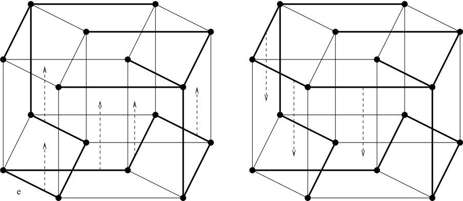
Our construction of the retraction from to depended on the fact that a spanning tree of with edges in direction has precisely -slidable edges, which may all be slid independently (in the sense that sliding any one of them has no effect on the slidability of the others). In Figures 8 and 9 we show by example that this fails for . Consequently, the methods of this paper do not readily extend to count the spanning trees of for .
The tree on the left in Figure 8 has only two vertical edges, but five vertically slidable edges on the path joining them. When any one of these five edges is slid vertically the other four necessarily cease to be slidable, because the vertical edges are now disconnected downstairs. However, if the edge labelled is slid two vertically slidable edges are created upstairs, as seen in the tree on the right.
Figure 9 shows that even when a spanning tree has precisely -slidable edges, the -slides cannot necessarily be made independently. The tree on the left has three edges joining the upper and lower -cubes, and precisely two edges that may be slid from one -cube to the other. However, if both are slid the result is not a tree, as seen in the graph on the right.

References
- [1] O. Bernardi. On the spanning trees of the hypercube and other products of graphs. E-print arXiv:1207.0896v3 [math.CO], 2012.
- [2] W. Goddard and H.C. Swart. Distances between graphs under edge operations. Discrete Math., 161(1-3):121–132, 1996.
- [3] L. Henden. The edge slide graph of the 3-cube. Rose-Hulman Undergraduate Mathematics Journal, 12(2), 2011. http://www.rose-hulman.edu/mathjournal/v12n2.php.
- [4] J.L. Martin and V. Reiner. Factorizations of some weighted spanning tree enumerators. J. Comb. Theory Ser. A, 104(2):287–300, 2003.
- [5] J.W. Moon. Various proofs of Cayley’s formula for counting trees. In A seminar on Graph Theory, pages 70–78. Holt, Rinehart and Winston, 1967.
- [6] K. Ozeki and T. Yamashita. Spanning trees: a survey. Graphs Combin., 27(1):1–26, 2011.
- [7] H. Prüfer. Neuer Beweis eines Satzes über Permutationen. Arch. Math. Phys., 27:742–744, 1918.
- [8] R.P. Stanley. Enumerative Combinatorics, Volume II. Number 62 in Cambridge Studies in Advanced Mathematics. Cambridge University Press, 1999.