Flows to Schrödinger Geometries

Abstract

We construct RG flow solutions interpolating AdS and Schrödinger geometries in Abelian Higgs models obtained from consistent reductions of type IIB supergravity and M-theory. We find that $z=2$ Schrödinger geometries can be realized at the minima of scalar potentials of these models, where a scalar charged under $U(1)$ gauge symmetry obtains a nonzero vacuum expectation value. The RG flows are induced by an operator deformation of the dual CFT. The flows are captured by fake superpotentials of the theories.

1 Introduction

Since the discovery of the AdS/CFT correspondence [1, 2, 3], there have been a lot of attempts to apply the correspondence to describe strongly coupled quantum field theories in terms of classical gravity. After the discovery, gravity duals of relativistic theories were considered at first. Now it also becomes important to consider applications to strongly coupled nonrelativistic systems. Gravity duals for nonrelativistic conformal field theories were constructed in Einstein gravity coupled to massive vector fields which break the relativistic conformal group to a nonrelativistic one [4, 5]. Soon after that, they were embedded into string/M theories using the so-called null Melvin twist solution generating technique [6, 7, 8]. These solutions are called Schrödinger geometry as the geometries have Schrödinger symmetry. Lifshitz geometry is also important for considering the gravity dual of nonrelativistic field theories, and is also obtained as a solution in the massive gauge theory [9, 10], which can be obtained from the Abelian Higgs model [11]. The embeddings to the string/M theories are worked out in [12, 13, 14, 15, 16, 17]. But the embedding of the Lifshitz geometries into string/M theory is more involved than that of the Schrödinger ones.

In this paper, we will consider a realization of the Schrödinger geometry in the Abelian Higgs models given by [18, 19], which are consistent truncations of type IIB SUGRA and M-theory.¹¹ 1 More general reductions, including these, are considered in [20, 21]. These models have W-shaped scalar potentials with two extrema at the origin and the nonzero point of a charged scalar field. The Abelian Higgs model is a massive gauge theory around the nonzero point, where the expectation value of the scalar field gives rise to the mass of the gauge field. Therefore, the Schrödinger geometry is expected to be realized there, while the asymptotically AdS space is obtained at the origin of the scalar potentials. It is, however, still nontrivial to embed the nonrelativistic geometries into these models since the parameters in the scalar potentials cannot be arbitrarily varied as opposed to effectively constructed bottom-up models. We will see that it is possible to find the Schrödinger solutions in both cases, while it is not possible for the Lifshitz solutions.

In particular, since the AdS and the Schrödinger geometries are realized in the maximum and the minimum of the potential, respectively, there must be an interpolating solution between them. We will construct such a solution, which is a domain-wall dual to the RG flow from a relativistic CFT in the ultraviolet (UV) to a nonrelativistic CFT in the infrared (IR).²² 2 In a different context, flow solutions from $AdS_{4}$ spacetime to the five-dimensional Schrödinger geometry have been constructed in M-theory in [22], whose IR geometry was obtained in [23]. See also [24, 25] for some related works on the geometric realization of Schrödinger symmetry. To trigger the RG flow, we will consider an addition of the deformation term $J{\cal O}$ to the UV theory, where $J$ is an external field coupled to the scalar operator ${\cal O}$ charged under a $U(1)$ symmetry. With this deformation, the $U(1)$ symmetry is supposed to be explicitly broken, and it is expected to flow to the other IR fixed point, where the IR geometry is the Schrödinger geometry in our case.

This paper is organized as follows. In Sec. 2, we review how to embed the Schrödinger geometry into the Abelian Higgs model, and then we consider the string/M theory construction of the Schrödinger geometries. In Sec. 3, we will construct the interpolating solutions. After discussing the asymptotics of the fields, we obtain domain-wall solutions numerically. We will discuss the puzzling aspects of our solutions and possible future directions in Sec. 4.

2 Schrödinger geometries from Abelian Higgs model

Gravity duals for nonrelativistic conformal field theories can be constructed in Einstein gravity coupled to massive vector fields [4, 5]. It is also pointed out that such massive gauge theories can be realized in the broken phase of Abelian Higgs models [5]. Let us summarize the construction briefly.

The metric of a gravity background dual to the boundary theories with Schrödinger symmetry is given by [4, 5]

\displaystyle ds^{2}=\ell^{2}\left[-\sigma^{2}r^{2z}(dx^{+})^{2}+\frac{dr^{2}}{r^{2}}+r^{2}(-dx^{+}dx^{-}+d\vec{x}^{2})\right]\ ,

(1)

where $z$ is the dynamical exponent, $\ell$ the radius, and $\sigma$ a parameter of the geometry. This arises from Einstein gravity coupled to a massive gauge field,

\displaystyle S=\frac{1}{16\pi G_{N}}\int d^{d+3}x\sqrt{-g}\left(R-2\Lambda-\frac{1}{4}F_{{\mu}{\nu}}F^{{\mu}{\nu}}-\frac{m^{2}}{2}A_{\mu}A^{\mu}\right)\ .

(2)

The solution (1) exists provided that the cosmological constant and the mass of the vector field are chosen as

\displaystyle\Lambda=-\frac{(d+1)(d+2)}{2\ell^{2}}\ ,\qquad m^{2}=\frac{z(z+d)}{\ell^{2}}\ ,

(3)

and that the gauge field takes the form

\displaystyle A_{+}=2\sigma\ell\sqrt{\frac{z^{2}-1}{z^{2}+8}}~r^{z}\ .

(4)

The massive gauge theory can be obtained in the broken phase of the Abelian Higgs model

\displaystyle S=\frac{1}{16\pi G_{N}}\int d^{d+3}x\sqrt{-g}\left(R-\frac{1}{4}F_{{\mu}{\nu}}F^{{\mu}{\nu}}-|(\partial_{\mu}-iqA_{\mu})\psi|^{2}-V(\psi)\right)\ ,

(5)

in which the scalar field $\psi$ obtains a nonzero vacuum expectation value (VEV) in the minima of the scalar potential $V(\psi)$ . The form of $\psi$ is restricted as $\psi=\psi_{0}e^{i\theta}$ , where $\psi_{0}\in\mathbb{R}$ corresponds to the vacuum expectation value of the scalar field. The phase $\theta$ can be absorbed by the gauge shift, and the resulting theory is the massive gauge theory,

\displaystyle S=\frac{1}{16\pi G_{N}}\int d^{d+3}x\sqrt{-g}\left(R-\frac{1}{4}F_{{\mu}{\nu}}F^{{\mu}{\nu}}-q^{2}\psi_{0}^{2}A_{\mu}A^{\mu}-V(\psi_{0}^{2})\right)\ .

(6)

It follows that the Schrödinger geometry can be obtained in the Abelian Higgs model (5) with the following parameters [5],

\displaystyle q^{2}\psi_{0}^{2}=\frac{z(z+d)}{2\ell^{2}}\ ,\qquad V(\psi_{0}^{2})=-\frac{(d+1)(d+2)}{\ell^{2}}\ .

(7)

We will consider the Schrödinger geometries in the models obtained from consistent truncations of ten-dimensional type IIB SUGRA and eleven-dimensional M-theory to five and four dimensions, respectively.³³ 3 More general solutions are constructed in [26], where the internal spaces are taken as Sasaki-Einstein manifolds, while they are squashed in our case. In both cases, we will obtain the solutions with the dynamical exponent $z=2$ .

2.1 In IIB string theory

Let us start from the five-dimensional case of type IIB SUGRA. The action contains a metric, a $U(1)$ gauge field, and a scalar [18],⁴⁴ 4 Here we rescaled the gauge field $A_{ours}=\frac{2L}{\sqrt{3}}A_{theirs}$ to normalize the coefficient of the field strength.

	$\displaystyle S=\frac{1}{16\pi G_{N}}$	$\displaystyle\int d^{5}x\sqrt{-g}\Big[R-\frac{1}{4}F^{2}+\frac{1}{12\sqrt{3}}\epsilon^{\lambda{\mu}{\nu}\sigma\rho}F_{\lambda{\mu}}F_{{\nu}\sigma}A_{\rho}$
		$\displaystyle\qquad-\frac{1}{2}(\partial_{\mu}\eta)^{2}-\frac{\sinh^{2}\eta}{2}(\partial_{\mu}\theta-\frac{\sqrt{3}}{L}A_{\mu})^{2}+\frac{3}{L^{2}}\cosh^{2}\frac{\eta}{2}(5-\cosh\eta)\Big]\ .$		(8)

This action is derived from a consistent truncation of a ten-dimensional IIB SUGRA action by decomposing the metric as

\displaystyle ds^{2}=\cosh\frac{\eta}{2}ds_{5}^{2}+\frac{L^{2}}{\cosh\frac{\eta}{2}}\left[ds_{V}^{2}+\cosh^{2}\frac{\eta}{2}(\zeta^{A})^{2}\right]\ ,

(9)

where $V$ is a four-dimensional Kähler-Einstein manifold with $R_{{\mu}{\nu}}=6g_{{\mu}{\nu}}$ , and $\zeta^{A}=\zeta+\frac{A}{\sqrt{3}L}$ and $\zeta=d\psi+\sigma$ such that $d\zeta=2\omega$ , with $\omega$ being a Kähler form [18]. The phase $\theta$ can be absorbed by the gauge shift. The Chern-Simons term can be ignored when the gauge field is assumed as $A\sim dx^{+}$ . The potential minima for the scalar field $\eta$ are at

\displaystyle\eta=\pm\log(2+\sqrt{3})\ .

(10)

The positive sign in (10) is chosen without loss of generality. The action reduces to the massive gauge theory around the minima, where the radius, the cosmological constant, and the mass of the gauge field are read off as

\displaystyle\ell^{2}=\frac{8}{9}L^{2}\ ,\qquad\Lambda=-\frac{27}{4L^{2}}\ ,\qquad m^{2}=\frac{9}{L^{2}}\ .

(11)

Comparing them with (3), the $z=2$ Schrödinger geometry is obtained in this model.⁵⁵ 5 There exists the other solution of (3) with $z=-4$ . We do not adopt it here. This solution is not supersymmetric because the $U(1)$ fibration of the internal manifold is stretched and there is no Killing spinor on it [27], as is mentioned in [18] for the AdS solution.

2.2 In M-theory

Similarly we can use a four-dimensional theory obtained from a consistent truncation of M-theory on a seven-dimensional Sasaki-Einstein manifold [19, 28],

	$\displaystyle S=\frac{1}{16\pi G_{N}}$	$\displaystyle\int d^{4}x\sqrt{-g}\Big[R-\frac{1}{4}F^{2}-\frac{1}{2}(\partial_{\mu}\eta)^{2}$
		$\displaystyle\qquad-\frac{\sinh^{2}\eta}{2}(\partial_{\mu}\theta-\frac{1}{L}A_{\mu})^{2}+\frac{1}{L^{2}}\cosh^{2}\frac{\eta}{2}(7-\cosh\eta)\Big]\ .$		(12)

Here we need a constraint for the gauge field $F\wedge F=0$ , but this is always satisfied for the Schrödinger background. The potential minima are at

\displaystyle\eta=\pm\log(3+2\sqrt{2})\ ,

(13)

and we find the massive vector theory with the parameters

\displaystyle\ell^{2}=\frac{3}{4}L^{2}\ ,\qquad\Lambda=-\frac{4}{L^{2}}\ ,\qquad m^{2}=\frac{8}{L^{2}}\ .

(14)

Then we obtain $z=2$ by solving (3) and (14).⁶⁶ 6 $z=-3$ is the other solution which satisfies (3). This solution is also nonsupersymmetric for a reason similar to the type IIB case [29, 30].

2.3 Comment on Lifshitz solutions

The massive vector theory also allows us to construct Lifshitz solutions of the form [9, 10]

\displaystyle ds^{2}=-\left(\frac{r}{\ell}\right)^{2z}dt^{2}+\ell^{2}\frac{dr^{2}}{r^{2}}+\left(\frac{r}{\ell}\right)^{2}d{\vec{x}_{d+1}}^{2}\ ,

(15)

by tuning the parameters such that

\displaystyle\Lambda=-\frac{z^{2}+dz+(d+1)^{2}}{2\ell^{2}}\ ,\qquad m^{2}=\frac{2z}{\ell^{2}}\ .

(16)

However, there are no physical solutions in the four- and five-dimensional theories considered above. It would be interesting to look for a consistent truncation which affords parameters consistent with the relations (16).

3 Domain-wall solutions

The actions given by (8) and (12) in five and four dimensions, respectively, have two vacua: one is supersymmetric at $\eta=0$ , and the other is nonsupersymmetric at $\eta=\eta_{\ast}\neq 0$ . As already studied in [21, 31], domain-wall solutions interpolating two AdS vacua can be constructed. Here we expect a domain-wall solution interpolating the AdS and the Schrödinger geometries.

We assume the following ansatz for the domain-wall solution,

$\displaystyle ds^{2}=$	$\displaystyle L^{2}\left(d\rho^{2}+e^{2A(\rho)}((d{x^{i}})^{2}-dx^{+}dx^{-})-B(\rho)e^{2zA(\rho)}(dx^{+})^{2}\right)\ ,$
$\displaystyle A_{+}$	$\displaystyle=La(\rho)e^{zA(\rho)}\ ,$	(17)
$\displaystyle\eta$	$\displaystyle=\eta(\rho)\ ,$

where $i=1,\dots,d$ , and $d=2$ and $d=1$ for type IIB and M-theory, respectively. This ansatz is chosen such that the Schrödinger geometry in the IR will become manifest. We focus only on the case of zero temperature, and an operator deformation will be assumed in the UV. The equations of motion are given by

$\displaystyle\eta^{\prime\prime}+(d+2)A^{\prime}\eta^{\prime}-\partial_{\eta}V_{pot}$	$\displaystyle=0\ ,$
$\displaystyle 2(d+1)A^{\prime\prime}+(d+1)(d+2)A^{\prime 2}+\frac{1}{2}\eta^{\prime 2}+V_{pot}$	$\displaystyle=0\ ,$	(18)
$\displaystyle(d+1)(d+2)A^{\prime 2}-\frac{1}{2}\eta^{\prime 2}+V_{pot}$	$\displaystyle=0\ ,$

where $V_{pot}$ is a scalar potential for $\eta$ ,

	$\displaystyle B^{\prime\prime}+(4z+d-2)A^{\prime}B^{\prime}-\Big[2(d+2-z)A^{\prime\prime}-2(2z^{2}+(d-2)z-\frac{d^{2}+5d+2}{2})A^{\prime 2}+\frac{1}{2}$	$\displaystyle\eta^{\prime 2}+V_{pot}\Big]B$
	$\displaystyle=\frac{d(d+1)}{2}a^{2}\sinh^{2}\eta+(zaA^{\prime}$	$\displaystyle+a^{\prime})^{2}\ ,$		(19)

and the Maxwell equation is

\displaystyle a^{\prime\prime}+(2z+d)A^{\prime}a^{\prime}+\left[zA^{\prime\prime}+z(z+d)A^{\prime 2}-\frac{d(d+1)}{2}\sinh^{2}\eta\right]a=0\ .

(20)

The second-order differential equations in (18) can be written as first-order equations [32]. One of the equations (18) is not independent, and the two independent ones can be obtained as the Euler-Lagrange equations for the following functional:

\displaystyle E=\int_{-\infty}^{\infty}d\rho\,e^{(d+2)A(\rho)}\left[(\partial_{\rho}\eta)^{2}-2(d+1)(d+2)(\partial_{\rho}A)^{2}+2V_{pot}\right]\ .

(21)

When the potential for the scalar takes the form

\displaystyle V_{pot}=\frac{1}{2}(\partial_{\eta}{\cal W})^{2}-\frac{d+2}{4(d+1)}{\cal W}^{2}\ ,

(22)

the functional can be rewritten as

	$\displaystyle E=\int_{-\infty}^{\infty}d\rho\,$	$\displaystyle e^{4A(\rho)}\left[(\eta^{\prime}\mp\partial_{\eta}{\cal W})^{2}-2(d+1)(d+2)(A^{\prime}\pm\frac{1}{2(d+1)}{\cal W})^{2}\right]$
		$\displaystyle\pm 2e^{(d+2)A(\rho)}{\cal W}\big\|_{-\infty}^{\infty}\ .$		(23)

Then it gives two first-order equations of motion,

\displaystyle A^{\prime}=\mp\frac{1}{2(d+1)}{\cal W}\ ,\qquad\eta^{\prime}=\pm\partial_{\eta}{\cal W}\ .

(24)

Here the $\mathcal{W}$ is called as a “fake superpotential.”

Let us find out the asymptotic behavior of the fields which solve the equations of motion around $\rho=\pm\infty$ . We first consider the solution in the UV $(\rho\to\infty)$ . The scalar field $\eta$ and metric $A$ can be expanded as

	$\displaystyle\eta$	$\displaystyle=\eta_{(0)}e^{-\Delta_{-}\rho/L}+\eta_{(1)}e^{-\Delta_{+}\rho/L}+\cdots\ ,$
	$\displaystyle A$	$\displaystyle=\frac{\rho}{L}-A_{(0)}e^{-2\Delta_{-}\rho/L}+\cdots\ ,$		(25)

where $\Delta_{\pm}$ are the dimensions of $\eta$ given by the solutions of $\Delta(\Delta-d-2)=-m_{\eta}^{2}$ , where $m_{\eta}$ is the (negative) mass of $\eta$ . Dots in the expansion include further exponentially suppressed contributions. The presence of $\eta_{(0)}$ corresponds to a deformation of the CFT in the UV by a term $\eta_{(0)}\mathcal{O}$ in the Lagrangian of the boundary theory, and the RG flow is caused by this operator deformation. The equations of motion (24) relates $A_{(0)}$ with $\eta_{(0)}$ as

\displaystyle A_{(0)}=\frac{\eta_{(0)}^{2}}{8(d+1)}\ .

(26)

For the Maxwell equation (20), we obtain the behavior of the gauge field

\displaystyle a=a_{(1)}\,e^{-z\rho/L}+a_{(2)}e^{-(z+d)\rho/L}+\cdots\ ,

(27)

which is nothing but

\displaystyle A_{+}=L(a_{(1)}+a_{(2)}e^{-d\rho/L}+\cdots)\ .

(28)

Finally, the function $B$ takes the form

	$\displaystyle B$	$\displaystyle=B_{(0)}e^{-m_{-}\rho/L}+B_{(1)}e^{-m_{+}\rho/L}+\cdots\ ,$
	$\displaystyle m_{\pm}$	$\displaystyle=\frac{1}{2}\left[4z+d-2\pm\sqrt{(4z+d-2)^{2}-8(2z^{2}+(d-2)z-\frac{d^{2}+5d+2}{2})+4V_{UV}L^{2}}\right]\ ,$		(29)

where $V_{UV}$ is the value of the potential at $\rho=\infty$ , and here we have used the fact that $\eta^{\prime}=0$ there.

It is straightforward also to find the asymptotic behavior of the fields in the IR $(\rho\to-\infty)$ . We impose the following boundary condition:

$\displaystyle\eta$	$\displaystyle=\eta_{\ast}+\widetilde{\eta}_{(0)}e^{\widetilde{\Delta}_{-}\rho/\ell}+\widetilde{\eta}_{(1)}e^{\widetilde{\Delta}_{+}\rho/\ell}+\cdots\ ,$
$\displaystyle A$	$\displaystyle=\frac{\rho}{\ell}-\widetilde{A}_{(0)}e^{2\widetilde{\Delta}_{-}\rho/\ell}+\cdots\ ,$
$\displaystyle a$	$\displaystyle=a_{0}+\cdots\ ,$
$\displaystyle B$	$\displaystyle=a_{0}^{2}+\cdots\ ,$	(30)

where $\eta_{\ast}$ is the vacuum expectation value of the scalar field at the minimum of the potential, and $\widetilde{\Delta}_{\pm}$ is the dimension of $\eta$ in the IR. The fake superpotential ${\cal W}$ defined by (22) will be convenient to read off $\widetilde{\Delta}_{\pm}$ . To derive the asymptotic forms of $a$ and $B$ in (30), we solved the equations of motion of IIB SUGRA (8) and M-theory (12) around the potential minimum. The constant $a_{0}$ appearing in the leading terms of $a$ and $B$ is responsible for the emergence of Schrödinger geometry in the IR. We will numerically solve the equations of motion to find domain-wall solutions with nonzero $a_{0}$ .

3.1 Fake superpotential and asymptotic solution

For concreteness, we compute coefficients appearing in the exponents of the asymptotic expansion for our IIB SUGRA and M-theory cases. We shall set the AdS radius $L=1$ for simplicity hereafter. In the computation, it is worthwhile to notice that the fake superpotential is useful to capture the RG flows and to determine the asymptotics.

We first consider the IIB SUGRA case, where $d=2$ and the domain-wall solution we focus on has $z=2$ . We can solve (22) to obtain a fake superpotential, as shown in Fig. 1, which corresponds to the RG flow induced by the scalar source $\eta_{(0)}$ in the UV and flowing to the vacuum at $\eta=\eta_{\ast}$ in the IR. The superpotential can be expanded around $\eta=0$ as $\mathcal{W}=-6-\eta^{2}/2+\cdots$ , and we see that the leading behavior of $\eta$ around $\rho=\infty$ corresponds to $\Delta_{-}=1$ . Since $V_{UV}=-12$ at the UV critical point $\eta=0$ , we obtain $m_{-}=2$ from (29). At the other critical point in the IR, $\eta_{\ast}=\log(2+\sqrt{3})$ , the superpotential in Fig. 1 can be expanded as

\displaystyle\mathcal{W}=-\frac{9}{\sqrt{2}}+\frac{3(\sqrt{6}-\sqrt{2})}{4}(\eta-\eta_{*})^{2}+\cdots\ ,

(31)

and then we obtain $\widetilde{\Delta}_{-}=2\sqrt{3}-2$ .

Refer to caption — Figure 1: The fake superpotential interpolating supersymmetric $(\eta=0)$ and nonsupersymmetric $(\eta=\eta_{\ast})$ vacua in IIB SUGRA (left panel) and M-theory (right panel).

We can repeat this analysis also in the M-theory case, where $d=1$ , $z=2$ , $V_{UV}=-6$ . In the UV, we have $\Delta_{-}=1$ , and (29) gives $m_{-}=2$ . Around the IR critical point, $\eta_{\ast}=\log(3+2\sqrt{2})$ , the superpotential can be expanded as

\displaystyle\mathcal{W}=-\frac{8}{\sqrt{3}}+\frac{(\sqrt{11}-\sqrt{3})}{2}(\eta-\eta_{*})^{2}+\cdots\ ,

(32)

and then we obtain $\widetilde{\Delta}_{-}=(\sqrt{33}-3)/2$ .

As the asymptotic behavior in the UV is obtained, it is convenient to rewrite the metric (17) so that the AdS geometry is manifest there. The ansatz (17) can be written as

\displaystyle ds^{2}=L^{2}\left[d\rho^{2}+e^{2A(\rho)}\left(-H(\rho)\left(dx^{+}+\frac{dx^{-}}{2H(\rho)}\right)^{2}+\frac{(dx^{-})^{2}}{4H(\rho)}+(d{x^{i}})^{2}\right)\right]\ ,

(33)

where $H(\rho)\equiv B(\rho)e^{2(z-1)A(\rho)}$ . Since $A(\rho)\to r/L$ and $\ B\to B_{(0)}e^{-2r/L}$ as $\rho\to\infty$ for both the IIB SUGRA and the M-theory cases $(z=2)$ , we find $H(\rho)\to B_{(0)}$ in the UV.⁷⁷ 7 It is not suitable to write the metric as in the form (33) in the IR because $H(\rho)\to 0$ as $\rho\to-\infty$ . Hence the metric in UV is AdS,

\displaystyle ds^{2}=L^{2}\left[d\rho^{2}+e^{2\rho/L}\left(-d\tau^{2}+d\sigma^{2}+(d{x^{i}})^{2}\right)\right]\ ,

(34)

where $\tau\equiv B_{(0)}^{1/2}x^{+}+B_{(0)}^{-1/2}x^{-}/2$ and $\sigma\equiv B_{(0)}^{-1/2}x^{-}/2$ . The coefficient $B_{(0)}$ , which will be obtained from numerical solutions and should be of order-one, is related to this “twisting” of the AdS geometry to generate the Schrödinger geometry.

3.2 Numerical solutions

We solve the equations of motion numerically by using the shooting method to obtain domain-wall solutions. We begin with the case of the IIB SUGRA, and will go back to the M-theory case after that. We focus only on the leading behavior of the asymptotic behavior of the fields in the UV and the IR. The subleading terms could be computed with sufficient numerical accuracy.⁸⁸ 8 This might be interesting from the point of view of the thermodynamic relation in the Appendix.

We have one parameter whose value can be chosen as the initial condition in the UV: $\eta_{(0)}$ . There is a scaling symmetry that allows us to set $a_{(1)}=1$ without loss of generality unless it is zero. Given this, we can obtain a domain-wall solution where the IR geometry is the Schrödinger geometry whose IR behavior is characterized by the value of $a_{0}$ . We will show that the $a_{0}$ is simply determined as a function of $\eta_{(0)}$ .

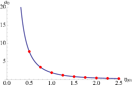
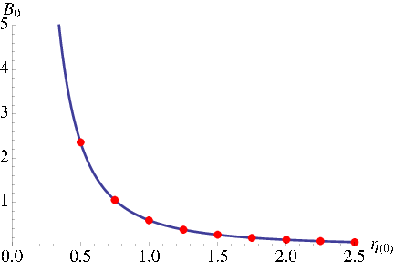
Figure 2 shows the domain-wall solution in the five-dimensional SUGRA (8) with $\eta_{(0)}=1$ . In the IR, the $a_{0}$ and $B$ grow along with $\eta$ , and the domain-wall solution interpolate the AdS in the UV and the Schrödinger geometry in the IR. In the absence of the gauge field, the IR geometry is just another lightlike AdS where the theory is in a nonsupersymmetric vacuum. The choice of $\eta_{(0)}$ in Fig. 2 is just for demonstration, so it is interesting to see how $a_{0}$ behaves when $\eta_{(0)}$ is varied. The result is shown in Fig. 3, and we find that the plot points can be fitted by $a_{0}=1.95/\eta_{(0)}^{2}$ and $B_{(0)}=0.588/\eta_{(0)}^{2}$ .

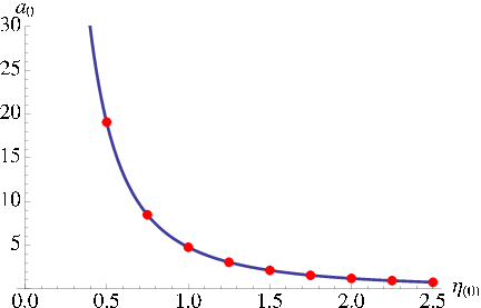
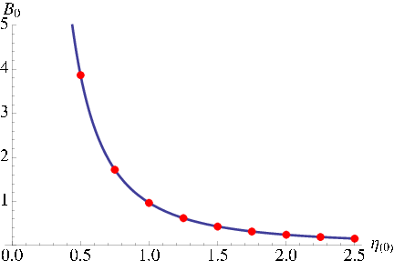
The domain-wall solution in the case of M-theory can be computed in a similar way as in the case of type IIB SUGRA. The solution is shown in Fig. 4, where $\eta_{(0)}=3/2$ is chosen as a demonstration. We find that $a_{0}$ is given as a function of $\eta_{(0)}$ , $a_{0}=4.77/\eta_{(0)}^{2}$ , and $B_{(0)}=0.967/\eta_{(0)}^{2}$ is obtained.

The Ricci scalar and the Kretschmann scalar are regular and monotonic functions of $\rho$ along the RG flow. In the type IIB SUGRA case, $R=-20/L^{2}$ and $R_{\mu\nu\rho\sigma}R^{\mu\nu\rho\sigma}=40/L^{4}$ in the UV, and $R=-22.5=-20/\ell^{2}$ and $RR=50.625=40/\ell^{4}$ in the IR. This agrees with the case of AdS-AdS domain-walls.

4 Discussions

We constructed RG flow solutions interpolating AdS and Schrödinger geometries by using Abelian Higgs models obtained in type IIB supergravity and in M-theory. We found that $z=2$ Schrödinger geometries are realized at the minima of the scalar potential of these models, where the scalar field obtained a nonzero vacuum expectation value, while it was not possible to embed the Lifshitz geometries into these models. The Lifshitz geometry has been constructed in four-dimensional ${\cal N}=2$ SUGRA [16, 17] which can be lifted to string/M-theory (see also [13, 15]). It would be interesting to investigate consistently truncated Abelian Higgs models which allow the Lifshitz geometries as solutions.

The RG flow was of the type induced by a scalar field source $\eta_{(0)}$ in the UV, corresponding to an operator deformation of the dual CFT. The solution is a one-parameter family of $\eta_{(0)}$ , and the IR value of the massive gauge field was controlled by $\eta_{(0)}$ . What we obtained can be phrased as a realization of emergent nonrelativistic symmetry in the IR at zero temperature. Our solution, however, is singular when the deformation is turned off, $\eta_{(0)}=0$ , as was shown in Figs. 3 and 5. This implies that our RG flow solutions cannot be obtained as a deformation of the AdS-AdS domain walls of [28] despite the fact that both are the solutions of the same theory. It will be interesting to see how the domain-wall solution we obtained is related to the context of holographic superconductors [33, 34]. The domain-wall solution here is induced by the operator deformation in the UV. On the other hand, a nonzero chemical potential gives VEVs to the operator dual to the scalar in the context of holographic superconductors. It will be challenging to construct the Schrödinger geometry by the RG flow induced by the VEV deformation in the UV. Our solutions would be a special limit of the anisotropic domain walls recently constructed in [35, 36], which might provide us with a clear understanding of the dual theories of our solutions.

Since the boundary is the AdS spacetime, we would be able to carry out holographic renormalization to understand the features of the dual field theory.⁹⁹ 9 A holographic renormalization on the Schrödinger geometries was discussed in [37]. Our solutions are similar to the GPPZ flow [38], where the gravity dual of an operator deformation of ${\cal N}=4$ SYM was studied. The holographic renormalization of the GPPZ flow was carefully carried out in [39], and it is straightforward to repeat the same analysis for our cases. Incongruously, the $U(1)$ current is conserved despite the operator deformation. This might be because the expectation value of the $U(1)$ charged operator dual to the source $\eta_{(0)}$ would be zero, i.e., $\eta_{(1)}=0$ . The value of the $\eta_{(1)}$ is completely determined by the behavior of the superpotential around $\eta=0$ . Although the superpotential we used is numerically generated and does not have a good asymptotic expansion around $\eta=0$ , the $\eta_{(1)}$ is likely to be zero within the numerical error. Another hint for the existence of the $U(1)$ symmetry is the conserved current we found in the Appendix that results from the scaling symmetry of our solutions. The conserved current could be interpreted as the thermodynamic relation of the dual field theory, and there might be a conserved charge of the form (47) that apparently comes from the bulk gauge field. Unfortunately, the usual procedure of holographic renormalization does not give us such a contribution since the Maxwell action vanishes when the on-shell solution is substituted. To obtain a nonzero contribution to the on-shell Maxwell action, the $A_{-}$ component on the lightlike AdS spacetime will be necessary. It is not clear how to account for the conservation of the $U(1)$ current (coming from the bulk gauge symmetry) as well as the conserved charge (47) in the thermodynamic relation [this is not necessarily the same as the $U(1)$ symmetry mentioned above]. Our solutions might be a singular limit of general solutions including the $A_{-}$ component, so it would be necessary to relax our ansatz to clarify the property of our solutions.

Acknowledgements

We are grateful to K. Murata, K. Skenderis, Y. Tachikawa and M. Taylor for valuable discussions. The work of T. N. was supported in part by the U.S. NSF under Grants No. PHY-0844827 and No. PHY-0756966.

Appendix A Conserved charges and thermodynamic relation

We would like to evaluate the conserved charges from our solutions that are asymptotically AdS space. We follow the argument given in Appendix C.2 of [6]. Given the Fefferman-Graham coordinates of the $AdS_{D+1}$ space

\displaystyle ds^{2}_{D+1}=L^{2}(d\rho^{2}+e^{2\rho}g_{ab}(x,\rho)dx^{a}dx^{b})\ ,

(35)

where $g_{ab}$ has the following expansion form

\displaystyle g(x,\rho)=g_{(0)}+g_{(2)}e^{-2\rho}+\cdots+g_{(D)}e^{-D\rho}-2h_{(D)}\rho e^{-D\rho}+\cdots\ ,

(36)

the coefficient $h_{(D)}$ is related to the Weyl anomaly of the boundary field theory, and the boundary stress-energy tensor reads

\displaystyle T_{ab}=\frac{DL}{16\pi G_{N}}(g_{(D)})_{ab}\ ,

(37)

for the flat boundary $(g_{(0)})_{ab}=\eta_{ab}$ [40, 41]. In our ansatz (17), the metric becomes asymptotically lightlike AdS space by shifting the coordinates as follows:

\displaystyle\tilde{x}^{+}=x^{+}\ ,\qquad\tilde{x}^{-}=x^{-}+B_{(0)}x^{+}\ .

(38)

The stress-energy tensor vanishes, except for the $++$ component

\displaystyle T_{++}=-\frac{(d+2)L}{16\pi G_{N}}B_{(1)}\ .

(39)

Then, the energy density and the particle number density, associated with the Killing vectors $\partial_{\tilde{x}^{+}}$ and $\partial_{\tilde{x}^{-}}$ , respectively, are

\displaystyle{\cal E}=T_{++}=-\frac{(d+2)L}{16\pi G_{N}}B_{(1)}\ ,\qquad{\cal N}=0\ .

(40)

One can find the conserved current in a similar manner to [42],

\displaystyle j=e^{dA}\left(e^{2A}(e^{2(z-1)A}B)^{\prime}-\phi\phi^{\prime}\right)\ ,\qquad\phi\equiv e^{zA}a\ ,

(41)

which satisfies $\partial_{\rho}j(\rho)=0$ up to the equations of motion. It is associated with the scale invariance of the solution of the form (17),

\displaystyle A\to A-\log\lambda\ ,\qquad x^{i}\to\lambda x^{i}\ ,\qquad x^{+}\to\lambda^{z}x^{+}\ ,\qquad x^{-}\to\lambda^{2-z}x^{-}\ .

(42)

The conservation of the current gives rise to the relation between the parameters in the UV and IR regions,

\displaystyle j(\rho=\infty)=j(\rho=-\infty)\ .

(43)

This gives us an additional constraint for the parameters as follows:

\displaystyle\frac{d+2}{d}B_{(1)}=a_{(1)}a_{(2)}\ .

(44)

In the nonrelativistic scale-invariant theory, the energy density and pressure are related by

\displaystyle z{\cal E}=d{\cal P}\ .

(45)

Then, the thermodynamic relation gives rise to

\displaystyle\frac{d+z}{d}{\cal E}=T{\cal S}+\mu{\cal Q}\ ,

(46)

where $T$ and ${\cal S}$ are the temperature and entropy density, and $\mu$ and ${\cal Q}$ are the chemical potential and charge density associated with some symmetry, respectively. Since there is no temperature in our solutions and $B_{(1)}$ is proportional to the energy density ${\cal E}$ , we obtain the following relation

\displaystyle\mu{\cal Q}=-\frac{(d+2)L}{16\pi G_{N}}a_{(1)}a_{(2)}\ .

(47)

This implies the existence of a conserved charge in our solutions, but the $U(1)$ symmetry is supposed to be explicitly broken by the operator deformation. We have the particle number symmetry in our solutions, and the density is zero as was given in (40). Then there seems to be no charges corresponding to (47).

This thermodynamic relation is unchanged in the $(\tau,\sigma)$ -coordinate. The components of the gauge field in this coordinate can be identified as $A_{\tau}=B_{(0)}^{-1/2}A_{+}$ and $A_{\sigma}=-B_{(0)}^{-1/2}A_{+}$ in $\rho\to\infty$ , and hence the asymptotic behavior of $A_{\tau}$ is

\displaystyle A_{\tau}=L(a_{(1)}B_{(0)}^{-1/2}+a_{(2)}B_{(0)}^{-1/2}e^{-d\rho/L}+\cdots)\ .

(48)

On the other hand, the expansion of the metric gives $g_{(D)\tau\tau}=B_{(1)}/B_{(0)}$ . Therefore, (44) is not disrupted by the coordinate transformation. In the $(\tau,\sigma)$ coordinates, the situation is that the $A_{\sigma}$ as well as the $A_{\tau}$ are turned on in the UV.

References

[1] J. M. Maldacena, The Large $N$ Limit of Superconformal Field Theories and Supergravity, Adv. Theor. Math. Phys. 2 (1998) 231–252, [hep-th/9711200].
[2] S. S. Gubser, I. R. Klebanov, and A. M. Polyakov, Gauge Theory Correlators from Non-Critical String Theory, Phys. Lett. B428 (1998) 105–114, [hep-th/9802109].
[3] E. Witten, Anti-de Sitter Space and Holography, Adv. Theor. Math. Phys. 2 (1998) 253–291, [hep-th/9802150].
[4] D. T. Son, Toward an AdS/Cold Atoms Correspondence: a Geometric Realization of the Schrödinger Symmetry, Phys. Rev. D78 (2008) 046003, [arXiv:0804.3972].
[5] K. Balasubramanian and J. McGreevy, Gravity Duals for Non-Relativistic CFTs, Phys. Rev. Lett. 101 (2008) 061601, [arXiv:0804.4053].
[6] J. Maldacena, D. Martelli, and Y. Tachikawa, Comments on String Theory Backgrounds with Non- Relativistic Conformal Symmetry, JHEP 10 (2008) 072, [arXiv:0807.1100].
[7] C. P. Herzog, M. Rangamani, and S. F. Ross, Heating Up Galilean Holography, JHEP 11 (2008) 080, [arXiv:0807.1099].
[8] A. Adams, K. Balasubramanian, and J. McGreevy, Hot Spacetimes for Cold Atoms, JHEP 11 (2008) 059, [arXiv:0807.1111].
[9] S. Kachru, X. Liu, and M. Mulligan, Gravity Duals of Lifshitz-Like Fixed Points, Phys. Rev. D78 (2008) 106005, [arXiv:0808.1725].
[10] M. Taylor, Non-Relativistic Holography, arXiv:0812.0530.
[11] S. S. Gubser and A. Nellore, Ground States of Holographic Superconductors, Phys. Rev. D80 (2009) 105007, [arXiv:0908.1972].
[12] K. Balasubramanian and K. Narayan, Lifshitz Spacetimes from AdS Null and Cosmological Solutions, JHEP 08 (2010) 014, [arXiv:1005.3291].
[13] A. Donos and J. P. Gauntlett, Lifshitz Solutions of D=10 and D=11 supergravity, JHEP 1012 (2010) 002, [arXiv:1008.2062].
[14] R. Gregory, S. L. Parameswaran, G. Tasinato, and I. Zavala, Lifshitz Solutions in Supergravity and String Theory, JHEP 12 (2010) 047, [arXiv:1009.3445].
[15] A. Donos, J. P. Gauntlett, N. Kim, and O. Varela, Wrapped M5-Branes, Consistent Truncations and AdS/Cmt, JHEP 12 (2010) 003, [arXiv:1009.3805].
[16] D. Cassani and A. F. Faedo, Constructing Lifshitz solutions from AdS, JHEP 1105 (2011) 013, [arXiv:1102.5344].
[17] N. Halmagyi, M. Petrini, and A. Zaffaroni, Non-Relativistic Solutions of N=2 Gauged Supergravity, JHEP 1108 (2011) 041, [arXiv:1102.5740].
[18] S. S. Gubser, C. P. Herzog, S. S. Pufu, and T. Tesileanu, Superconductors from Superstrings, Phys. Rev. Lett. 103 (2009) 141601, [arXiv:0907.3510].
[19] J. P. Gauntlett, J. Sonner, and T. Wiseman, Holographic Superconductivity in M-Theory, Phys. Rev. Lett. 103 (2009) 151601, [arXiv:0907.3796].
[20] J. P. Gauntlett and O. Varela, Universal Kaluza-Klein Reductions of Type IIB to ${\mathcal{N}}\!=4$ Supergravity in Five Dimensions, JHEP 06 (2010) 081, [arXiv:1003.5642].
[21] D. Cassani, G. Dall’Agata, and A. F. Faedo, Type IIB Supergravity on Squashed Sasaki-Einstein Manifolds, JHEP 05 (2010) 094, [arXiv:1003.4283].
[22] H.-C. Kim, S. Kim, K. Lee, and J. Park, Emergent Schrödinger Geometries from Mass-Deformed CFT, JHEP 08 (2011) 111, [arXiv:1106.4309].
[23] E. O Colgain, O. Varela, and H. Yavartanoo, Non-Relativistic M-theory Solutions Based on Kähler- Einstein Spaces, JHEP 07 (2009) 081, [arXiv:0906.0261].
[24] H. Ooguri and C.-S. Park, Supersymmetric Non-Relativistic Geometries in M-theory, Nucl. Phys. B824 (2010) 136–153, [arXiv:0905.1954].
[25] J. Jeong, H.-C. Kim, S. Lee, E. O Colgain, and H. Yavartanoo, Schrodinger invariant solutions of M-theory with Enhanced Supersymmetry, JHEP 03 (2010) 034, [arXiv:0911.5281].
[26] A. Donos and J. P. Gauntlett, Solutions of type IIB and D=11 supergravity with Schrodinger(z) symmetry, JHEP 0907 (2009) 042, [arXiv:0905.1098].
[27] L. J. Romans, New Compactifications of Chiral ${\mathcal{N}}\!=2$ D = 10 Supergravity, Phys. Lett. B153 (1985) 392.
[28] S. S. Gubser, S. S. Pufu, and F. D. Rocha, Quantum Critical Superconductors in String Theory and M- Theory, Phys. Lett. B683 (2010) 201–204, [arXiv:0908.0011].
[29] C. N. Pope and N. P. Warner, Two New Classes of Compactifications of D = 11 Supergravity, Class. Quant. Grav. 2 (1985) L1.
[30] C. N. Pope and N. P. Warner, An $SU(4)$ Invariant Compactification of D = 11 Supergravity on a Stretched Seven Sphere, Phys. Lett. B150 (1985) 352.
[31] J. P. Gauntlett, S. Kim, O. Varela, and D. Waldram, Consistent Supersymmetric Kaluza–Klein Truncations with Massive Modes, JHEP 04 (2009) 102, [arXiv:0901.0676].
[32] K. Skenderis and P. K. Townsend, Gravitational Stability and Renormalization-Group Flow, Phys. Lett. B468 (1999) 46–51, [hep-th/9909070].
[33] S. A. Hartnoll, C. P. Herzog, and G. T. Horowitz, Building a Holographic Superconductor, Phys. Rev. Lett. 101 (2008) 031601, [arXiv:0803.3295].
[34] S. A. Hartnoll, C. P. Herzog, and G. T. Horowitz, Holographic Superconductors, JHEP 12 (2008) 015, [arXiv:0810.1563].
[35] D. Arean, M. Bertolini, C. Krishnan, and T. Prochazka, Type IIB Holographic Superfluid Flows, JHEP 1103 (2011) 008, [arXiv:1010.5777].
[36] D. Arean, M. Bertolini, C. Krishnan, and T. Prochazka, Quantum Critical Superfluid Flows and Anisotropic Domain Walls, JHEP 1109 (2011) 131, [arXiv:1106.1053].
[37] M. Guica, K. Skenderis, M. Taylor, and B. C. van Rees, Holography for Schrödinger Backgrounds, JHEP 02 (2011) 056, [arXiv:1008.1991].
[38] L. Girardello, M. Petrini, M. Porrati, and A. Zaffaroni, The Supergravity Dual of ${\mathcal{N}}\!=1$ Super Yang-Mills Theory, Nucl. Phys. B569 (2000) 451–469, [hep-th/9909047].
[39] M. Bianchi, D. Z. Freedman, and K. Skenderis, Holographic Renormalization, Nucl. Phys. B631 (2002) 159–194, [hep-th/0112119].
[40] S. de Haro, S. N. Solodukhin, and K. Skenderis, Holographic Reconstruction of Spacetime and Renormalization in the AdS/CFT Correspondence, Commun. Math. Phys. 217 (2001) 595–622, [hep-th/0002230].
[41] K. Skenderis, Asymptotically Anti-de Sitter Spacetimes and Their Stress Energy Tensor, Int. J. Mod. Phys. A16 (2001) 740–749, [hep-th/0010138].
[42] I. R. Klebanov, S. S. Pufu, and T. Tesileanu, Membranes with Topological Charge and AdS4/CFT3 Correspondence, Phys. Rev. D81 (2010) 125011, [arXiv:1004.0413].