Gauge Mediated Supersymmetry Breaking in Five Dimensions
Moritz McGarrie
A Thesis presented for the degree of
Doctor of Philosophy
![[Uncaptioned image]](1109.6245v1/qmblue.png)
Centre for Research in String Theory
Department of Physics
Queen Mary
327 Mile End Road
England
August 2011
Gauge Mediated Supersymmetry Breaking in Five Dimensions
Moritz McGarrie
Submitted for the degree of Doctor of Philosophy
August 2011
Abstract
In this thesis we focus on the construction of models in which a supersymmetry breaking hidden sector is located on one fixed point of an extra dimensional interval and the effects are gauge mediated across this interval to the other fixed point where the supersymmetric standard model is located. We use the formalism of current correlators to encode supersymmetry breaking effects and explore flat, warped and deconstructed extra dimensions. We also apply these techniques to models of metastable supersymmetry breaking in Supersymmetric Quantum Chromodynamics.
Declaration
The work in this thesis is based on research carried out at the Centre for Research in String Theory, Queen Mary University of London. Except where specifically acknowledged in the text the work in this thesis is the original work of the author. Chapter 2 is based on the publication [1] with Rodolfo Russo and similarly chapter 6 is based on the publication [2] with Daniel C. Thompson. Additional results in this thesis are based on publications by the author [3, 4]. I also acknowledge a complementary publication with Steven Thomas and Daniel Koschade [5], the results of which are not included in this thesis.
Acknowledgements
I would like to thank Queen Mary, Centre for Research in String Theory and especially my supervisors Steven Thomas and Rodolfo Russo. I would like to thank John, Jane, Carolyn, Madeleine, Kirsten and Ian. I would like to thank Camilla and Lurpak for supporting my passion and finally to my friends and colleagues.
Chapter 1 Introduction
The Standard Model (SM) of particle physics is a widely accepted and accurately tested theory that describes the bosonic interactions of the strong, weak and electromagnetic forces between the fermionic quarks and leptons that make up the familiar and everyday world around us. It is a Lorentz invariant Quantum Field Theory (QFT) of gauge interactions. These standard model forces, are described by the exchange of excitations of bosonic gauge fields. The quarks and leptons are excitations of fermionic fields. Additionally, the standard model includes a Higgs scalar field. Unfortunately, as a theory it is sick and incomplete. Firstly there is nothing within the theory that determines the electroweak scale from which most of the theory relies. Secondly this scale, set by the Higgs mass, is extremely unstable under quantum corrections unless there is a fine tuning to the 38th decimal place [6]: the Hierarchy problem. Other criticisms may be mounted against it: the standard model makes no attempt to unify with the force of gravity and seems rather poor at explaining physics on large scales, such as the composition of Dark matter and Dark energy relative to the visible matter of the universe.
The Large Hadron Collider (LHC) at CERN is expected to test various extensions of the standard model of high energy physics. One very well motivated extension is supersymmetry (SUSY). Mathematically, the boson and fermion fields of the standard model are representations of the Lorentz symmetry group. The generators of this group are represented only by bosonic generators and . As there are bosonic and fermionic fields within the standard model, it is logical to suggest that the Lorentz symmetry group may be extended to include generators that are also fermionic: a supersymmetric quantum field theory. From a mathematical viewpoint, this is a rather innocuous suggestion. When taken as a serious description of nature it has some profound and far reaching consequences. Firstly, it predicts a supersymmetric standard model of particle physics, in which all known fields have superpartners, with differing spins. The constraints of the observed standard model on these unobserved fields leads to the conclusion that this symmetry, if it exists, is broken. Perhaps more profoundly, these constraints imply that it is broken in a local hidden sector that is not included within the standard model and that this breaking is then mediated to the supersymmetric standard model. Further, for this symmetry to be broken dynamically, and importantly to supply a natural hierarchy of scales, implies a hidden sector that is described by a strongly coupled gauge theory.
A softly broken supersymmetric standard model is a natural solution to many of the puzzles of the standard model such as the Hierarchy problem [7]. Additionally, supersymmetry has useful dark matter candidates which the most accurate astrophysical observations and the Cosmological model [8], Lambda CDM (the cosmological constant plus cold dark matter), predicts makes up of the universe, of which visible matter makes up only . Additional hints of supersymmetry arise from its enhancement of gauge coupling unification of the standard model as required by Grand Unified Theories (GUT) [9]. Finally, supersymmetry is a necessary component of superstring theory, which does supply a consistent framework from which the standard model and gravity may both arise.
This introductory chapter will motive the study of supersymmetry, its breaking and its mediation across and extra dimension via gauge interactions. Of course there are many alternative proposals for extensions of the standard model with or without supersymmetry and with or without extra dimensions. We will simply outline some of the guiding motivations for choosing this particular research direction.
1.1 Why Supersymmetry?
The (non supersymmetric) standard model, and in particular electroweak symmetry breaking, is unnatural [10, 11, 6, 12, 13] as a field theory as the Higgs mass is extremely unstable under quantum corrections unless there are finely tuned counterterms in its Ultra Violet (UV) completion. A straightforward calculation of the one loop correction to the physical Higgs field , two point function, from couplings with fermions, for instance top quarks 11 1 We are using four component notation here.
| (1.1) |
The complex scalar may be written as22 2 A different parameterisation is
| (1.2) |
where in unitary gauge where , gives a quadratically divergent integral, as well as logarithmically divergent one (to show this use and :
| (1.3) |
The divergence may be absorbed into counter terms leaving a finite correction to the propagator of order , which one may argue is not so fine tuned, albeit rather arbitrary. However, any UV GUT completion will inevitably introduce similar contributions whose mass scale is now , such that even the usual finite terms result in a cancellation between bare mass and renormalised mass to within a few GeV.
The introduction of superpartners for fermions33 3 see appendix A for superspace notaton, the complex scalars , , will generate couplings of the form
| (1.4) |
These provide additional contributions to the two point function:
| (1.5) |
Remarkably if the Yukawa coupling , the combined quadratic divergences from scalars and fermions cancel exactly, regardless of any of the mass scales introduced. The presence of supersymmetry in the Lagrangian naturally acts to remove quadratic divergences and are therefore rather soft. Remarkable also is that the remaining divergences depend on the mass splitting between fermion and sfermion masses such that if even the vacuum of the theory is supersymmetric, all divergences cancel exactly (with a little help from D.1.22):
| (1.6) |
In the superspace formalism (See appendix A) which we adopt throughout this thesis both Eqn. (1.1) and Eqn. (1.4) compactly arise from the superpotential
| (1.7) |
when computing the Yukawas and F-term potential, respectively. Extending the standard model with supersymmetry with two Higgs superfields for anomaly cancellation and to keep the superpotential holomorphic, plus terms that break supersymmetry softly as demonstrated above, is known as the Minimal Supersymmetric Standard Model (MSSM). The soft terms we may add to the MSSM are
| (1.8) |
This thesis will focus on the theoretical computation of the soft terms for scalars and the gauginos .
In summary, (1) The introduction of superpartners for scalars, in particular the Higgs of the standard model, protects these scalar fields from quadratic divergences in its self energy. (2) As long as the superpartners of a scalar have a similar mass to the scalar, the scalar mass is shielded from loop corrections from other heavier particles that may arise in any Grand Unified Theory (GUT) or higher dimensional extension of the standard model which may act as a UV completion. In summary, supersymmetry is a natural way to improve the standard model and protect electroweak physics from UV effects. It does not yet explain the electroweak scale.
1.2 Dynamical Supersymmetry Breaking
Dynamical supersymmetry breaking is a natural way to explain the electroweak scale:
“As was first suggested by Witten [14], we would like the mechanism which spontaneously breaks supersymmetry to be dynamical. This means that it arises from an exponentially small effect, and therefore it naturally leads to a scale of supersymmetry breaking, , which is much smaller than the high energy scales in the problem (which can be the Planck scale or the grand unified scale):
(1.9) This can naturally lead to hierarchies. For example, the weak scale can be dynamically generated, explaining why .”(From [15])
As the dynamics is strongly coupled, perturbation theory in the fundamental “quarks” and “gluons” is of little use here. However much more may be learned about the low energy dynamics by writing an effective Lagrangian which contains the low energy degrees of freedom and preserves the symmetries and interactions of the system. For instance the linear sigma model is used to describe mesons which encapsulate the collective behaviour of quarks and gluons at low energies. Corrections to the effective description are due to an expansion of operators in , where is the the momomenta and is the scale at which the fundamental variables become strongly coupled. The strongly coupled microscopic theory and the effective macroscopic theory are said to be within the same “Universality Class” as they both flow to the same infrared fixed point, within the space of dimensionless couplings. Precisely at the fixed point the descriptions are no longer effective, they are exact. This provides the notion that two (or more) descriptions may be dual. One description may offer a more useful perturbative description to examine its low energy properties. Equally one may start with dual descriptions and, by adding various operators or deformations, build useful effective descriptions. Further, one may on occasion make these flows arbitrarily close, such that the duality holds along an entire flow [16, 17].
Much progress has been made in understanding dynamical supersymmetry breaking via the use of dualities [18, 19, 16, 20, 21] and in particular Seiberg duality [22, 23], in which exactly dual descriptions can be found at conformal fixed points, which then become effective descriptions after adding deformations such as small quark masses in the “electric” or fundamental microscopic description. This progress has culminated in the viewpoint that supersymmetry is broken dynamically in a metastable minima [24], the ISS model, which is usually explored in its “magnetic” or IR-free description. This development in supersymmetry breaking is rather compelling and many questions seems to have a natural footing within this construction. For instance stability of the metastable broken vacuum is ensured by a parametrically small parameter
| (1.10) |
where is the quark mass scale and is the strong coupling scale. Stability also arises dynamically: the universe naturally cools towards a vacuum with more light degrees of freedom, and at lower temperatures the vacuum becomes trapped and parametrically long lived [25, 26]. GUT unification and its breaking may also be dynamically explained by the behaviour of the breaking of flavour symmetries of the hidden sector [5]. Additionally the potential between the two vacua of the ISS model [24] is generically long and flat, providing a natural candidate for inflation. Throughout this thesis we have in mind that supersymmetry is broken in this, or some related, way. What we hope to contribute, in this thesis, is a rigorous theoretical framework for analysing different methods of mediating this type of supersymmetry breaking. We will argue that we are compelled to suggest gauge mediation and in particular some sort of effective extra dimension, in which massive vector like objects participate in this mediation. We will discuss these issues further in chapters 3 and 6.
A perhaps alternate viewpoint due to Randall and Sundrum [27], as a solution to the Hierarchy problem, is when the geometry of spacetime generates a hierarchy of scales. Starting from the metric given by
| (1.11) |
is the AdS curvature scale, we may look at intervals of this space with with . Mass terms geometrically located at will be exponentially suppressed such that
| (1.12) |
In general, one still needs supersymmetry to protect this hierarchy. In fact it is rather enticing to suggest that if the local hidden sector that breaks supersymmetry dynamically is both approximately conformal and has a large gauge group, then one may construct a low energy effective Lagrangian via the AdS/CFT correspondence. One may then argue that the exponential warp factor is similarly capturing the dynamically generated hierachy of scales between supersymmetry breaking scale and that of the UV scale. The supersymmetric “slice of AdS” with supersymmetry breaking on the IR fixed point, mediated to the UV fixed point by gauge interactions may act as a powerful effective description of the period of approximately conformal running of the hidden sector gauge group. Importantly, fields that live in the full five dimensions will have a Kaluza-Klein (kk) mode expansion, with masses associated with the AdS warp factor, roughly due to the interval of length .
To be clear, we are not constructing an AdS description of the MSSM, but rather taking a conceptually different construction. For concreteness, we have in mind an , in the UV description. The is approximately conformal between the UV scale , down to some scale which will equate to the mass of the lightest kk mode. In the IR the breaks supersymmetry which is, essentially captured on the IR brane of the AdS dual description. This gauge group and matter content may admit an AdS dual low energy effective description, just as under Seiberg duality, a UV-free electric description admits an IR dual magnetic description. The is a global flavour symmetry for which some subgroup is weakly gauged and associated with the MSSM gauge group or parent GUT . The global currents of this flavour symmetry would in principle require all order corrections from the hidden sector in terms of the electric description, when in the IR (the currents in the electric desciption are well defined in the UV), but since we have a low energy effective description, we can in principle determine those corrections in terms of the dual variables. We also point out that QCD has well defined UV currents of the and global groups. In the IR, various tools are applied such as operator product expansions, sum rules, Padé approximations and AdS/QCD to determine the structure of these currents.
In particular, we should expect that on the IR brane, should be some O’Raifeartaigh type model [28], perhaps rather similar to the magnetic description of the ISS construction [24]. This is simply parameterised by currents located on the IR brane. Under the correspondence, a global symmetry of the CFT is interpreted as a gauge symmetry of the bulk and resonances of the CFT act as Kaluza-Klein modes of the gauge symmetry. On the CFT side, these fields should be thought of as part of the currents themselves, form factors, which on the AdS side appear as mediators of the IR brane localise currents. Most compelling in this construction is that as the gauge fields live in the bulk, Kaluza-Klein modes of the gauge fields will participate in the mediation of supersymmetry breaking. A closely related phenomena arises both in QCD as “Vector Meson Dominance” [29, 30] and also rather naturally, although most often a subleading effect, within ISS models themselves, whenever one embeds the standard model gauge groups within a flavour group that exhibits “magnetic colour-flavour locking” [31]. It may help conceptually to think of chapter 3 as capturing a truncated version of the AdS model we are suggesting, which includes only the first Kaluza-Klein modes and the IR brane supersymmetry breaking sector. We will return to these topics in chapters 3 and 6.
1.3 Why a Hidden Sector?
So far we have argued that supersymmetry protects the hierarchy of scales between the Planck scale and the electoweak scale and that dynamically broken supersymmetry arising from strong dynamics naturally generates this hierarchy in the form of the supersymmetry breaking. This equation is modified by the introduction of supergravity. In fact the constraints of supersymmetry require that the standard model does not directly participate in the breaking of supersymmetry and the argument is as follows:
In superspace notation, the supersymmetric standard model (SSM) action , will have a superpotential :
| (1.13) |
where . Where we have explicitly assumed a perturbative description with canonical Kähler potential. Through derivatives of the superpotential, one encodes fermion mass terms, scalar mass terms and Yukawa couplings. As a result these quantities are constrained and related. The upshot are some supertrace mass sum rules [32]:
| (1.14) |
with labelling the spin of the states. In fact this can be shown to be true over each chiral supermultiplet and including arbitrary gauge interactions [33]
| (1.15) |
These mass sum rules imply that if supersymmetry is broken within the SSM then for every standard model particle, there must be a superpartner with a mass lighter or equal to the standard model particle clearly ruled out by experiment [34]. These sum rules are protected as a consequence of the Nonrenormalisation theorem which states that the superpotential 1.13, which is holomorphic, does not receive any renormalisation at any order in perturbation theory. This theorem may be motivated intuitively by realising that all local44 4 in coordinate space loops written in superspace must have a minimum of two internal propagators or equivalently must appear, which is not holomorphic.
This leads to the requirement of a hidden sector where supersymmetry is broken. The hidden sector can supply the necessary explicit breaking soft terms, such as the gaugino and sfermion masses, necessary for the SSM superpartner masses and to evade the constraints of the sum rules. From the perspective of the visible sector, the soft terms explicitly break the sum rules however these terms may be generated by a supersymmetry breaking sector that necessarily obeys these sum rules.
1.4 Interlude: Form factors
The scattering part of the S-matrix between an ingoing state and an out going state is given by
| (1.16) |
If the external states are not fundamental, i.e. composite, we can therefore think of the matrix element as the definition of the current. Translation invariance allows us to define
| (1.17) |
The simplest example [35] is of the (4-component Dirac) electron. Inclusion of radiative corrections will give a result of the form
| (1.18) |
One may choose to contract with spinor wavefunctions to obtain a spin index contracted form factor. is a momentum dependent form factor (), which to lowest order and . In the Hadronic world, one may think of the electromagnetic and weak forces as “external fields”. The external probe fields therefore couple to Hadronic currents [36]. A simple example is that of the meson
| (1.19) |
What one finds experimentally is not , and additionally it is presumed that . In fact it is argued that if an intermediate meson is exchanged then from general considerations the form factor is
| (1.20) |
This is vector meson dominance. What is perhaps less obvious is that one may think of the meson as a Kaluza-Klein mode of the photon, such that the form factor is given by a bulk propagator. Schematically with and ,
| (1.21) |
That hadronic form factors appear from weakly gauged global symmetries of the UV theory, and that their form may be modelled by a gauge symmetry in some higher dimensional space, has lead to Hidden Local Symmetry models and AdS/QCD as a very compelling description of low energy QCD [29, 37, 38, 39, 40, 41]. We are strongly compelled to argue that this generic feature of strongly coupled gauge theories will manifest itself in interactions with a supersymmetry breaking hidden sector, including in the generation of soft terms for the MSSM.
1.5 Gauge Mediation
So far we have a picture of supersymmetry being broken in a sector that is not part of the Minimal Supersymmetric Standard Model (MSSM) and additionally we have a sensible dynamical method of breaking supersymmetry. The transmission of the supersymmetry breaking effects to the MSSM may arise from either gauge or gravitational interactions. In this thesis we shall explore gauge mediation and not comment further on gravity mediation.
1.5.1 General Gauge Mediation

General gauge mediation [42] can be defined as follows; In the limit that the standard model gauge couplings , labelling respectively, the theory decouples into three sectors: a sector that breaks SUSY, the MSSM matter and the gauge mediating sector, as in figure 1.1 . Strictly speaking, it is only necessary that the coupling the standard model/mediating sector decouple. Computations may be made perturbatively in the MSSM gauge couplings between . Typically, this construction may be achieved by first building a hidden sector such as the ISS construction and then weakly gauging a flavour symmetry of the hidden sector and associating this with the MSSM gauge groups. The currents and correlators of this weakly gauged global symmetry encode the supersymmetry breaking effects. Within this framework, one may look at variations on this theme by changing either of the three sectors [43, 44, 45, 46, 47, 48, 49, 50, 51, 52, 53, 54]. For the most part four dimensional models have focused on comparing different SUSY breaking sectors, i.e. different currents, whilst holding the other two sectors fixed. In this thesis we will change the mediating sector, whilst staying within the definition of general gauge mediation. In particular we would like to explore models where the mediating sector has Kaluza-Klein modes and for that we will explore both five dimensional models and deconstructed four dimensional ones.
There is an important additional point on the framework of GGM is that it allows strongly coupled hidden sectors to be encoded into current correlators so that they may be extensively studied. If the hidden sector is strongly coupled then in principle the current correlators must be known exactly with regard to . In this case the current correlators simply parameterise our ignorance in terms of the current correlators and we compute soft masses perturbatively in the ’s.
A far more powerful use of the current correlator framework arises from the use of dualities. As the hidden sector and visible sector completely decouple, one may use a dual description of the currents of the weakly gauged global symmetry, in terms of the effective variables. Within the ISS construction this naturally arises as one takes the two point functions of the magnetic degrees of freedom of the hidden sector even though the true fundamental current correlators are in terms of strongly coupled variables. In this thesis we will show that even truly four dimensional models, with regard to the microscopic description, may have an apparent extra dimensional structure, within the macroscopic description. This arises both in the sense of (De)constructed extra dimensions [3] and through the AdS/CFT correspondence [2]. Heuristically, in principle all-order current correlators on the left hand side may be factorisable:
| (1.22) |
such that it may be described by a current correlator of the effective degrees of freedom, multiplied by a momentum dependent form factor . The ellipses denote that the right hand side is a perturbative expansion in of the all-order current correlators on the right hand side. From the perspective of the weak side of the duality the form factor arises due to Kaluza-Klein modes of the vector superfield, with mass , participating in the mediation of supersymmetry. From the perspective of field theory these are vector-like resonances of the strongly coupled description. The form factor is associated with a bulk propagator
| (1.23) |
In this sense the GGM construction truly captures the essence that a four dimensional calculation on one side is equivalent to a 5d calculation on the other side of a duality transformation. For the particular case of a two site lattice model, we will show that this form factor is completely dominated by the first kk mode mass, and we recover exact vector meson dominance. In fact it is quite reasonable that this type of factorisable structure should occur under the duality, as both the four dimensional general gauge mediation [42] equations for the scalar masses should be valid and so should the five dimensional scalar mass equations of the dual five dimensional models.
This motivation for exploring extra dimensions, which may be understood by comparing with QCD physics. The strong force binding quarks as fundamental objects at high energies, is a gauge theory which at low energies has an effective description of baryons and mesons. In particular the vector like spin- mesons for example the octet containing mesons, appear to arise from a purely emergent local symmetry due to the effects of strong coupling [30, 29]. This symmetry is not apparent in the high energy quark description. In fact these resonances behave like the lightest Kaluza-Klein particles of an extra dimension. Not only are vector mesons detectable in experiment, they also influence many physical processes of the standard model through an effect known as “vector meson dominance” [55], whereby the form factor of interacting with electromagnetism, is dominated by the meson. If the hidden sector is strongly coupled, it seems likely that the analogue of vector mesons should arise in the low energy effective description and play an important role in phenomenology.
Gauge mediation in five dimensions captures the analogous effect. In the process of this thesis we will demonstrate how purely four dimensional models of SQCD may develop effective Kaluz-Klein modes analogous to mesons and that they act to screen scalar masses analogous to vector meson dominance. We will then show that by interpreting the hidden sector as having an effective AdS dual description, one may further capture similar features. All these developments will become more apparent in the later chapters: chapter 2 will simply focus on a rigorous five dimensional extension of general gauge mediation.
1.5.2 Gaugino Mediation and GGM5D
Typically in extra dimensional models of gauge mediation, the Kaluza-Klein modes of the vector multiplet participate in the mediation of supersymmetry. This acts to screen scalar masses of the MSSM, as was first shown rather rigorously by Mirabelli & Peskin [56] and is pictured in figure 1.2.

As a result, for a minimal hidden sector, typically the gaugino mass is the only non-zero soft term and additionally, gaugino mass contributions in the renormalisation group equations (RGE’s) [57, 58, 59] pictured in figure 1.3, will generate scalar masses for the MSSM. This was explored phenomenologically in models of Gaugino mediation [60, 61, 62, 63]. As the whole theory depends on only one soft term, it is rather predictive.

We would like to empasise that this is simply a particular, and minimal case, of a far broader space of possible five dimensional constructions. General gauge mediation in five dimensions may be shown to interpolate between the screened and unscreened (or four dimensional) limit of scalars masses, as is shown in chapter 5: Hybrid mediation. Further, as in general gauge mediation, both four and five dimensions, the gaugino and sfermion current correlators are not related, so it is rather simple to construct a model in which for example, the gaugino Majorana mass is vanishingly small through an approximate R-symmetry, the scalar masses are only partially screened in the Hybrid regime, and the erstwhile massless gaugino gets a Dirac mass instead [64]. This is just one example of the rich set of phenomenologically unexplored possibilities that we hope general gauge mediation in five dimensions may be applied to, which seem no more or less likely than the benchmark construction of Gaugino mediation. Additionally, we emphasise that general gauge mediation in five dimensions gives a natural geometric interpretation of the decoupling limit of GGM, as the hidden and visible sectors are spatially separated on different fixed points it makes direct couplings impossible by construction. Further, the screening effect on the scalar masses may alleviate many problems found in models of ISS [24] of anomalously light gauginos relative to scalars.
1.6 Chapter Summary
This chapter has summarised the motivations for a supersymmetric standard model in which supersymmetry breaking is described by a hidden sector and gauge mediated to the MSSM. We have also given an outline for this thesis in which we will focus on gauge mediated supersymmetry breaking across an extra dimension within the program of current correlators which allows for a model independent construction which is also applicable for analysing strongly coupled hidden sectors. The remaining of this thesis will work as follows: in chapter 2 we will outline the framework of using current correlators to encode brane to brane mediation of supersymmetry on a background. In chapter 3 we will demonstrate the utility of this framework by applying it to models of metastable supersymmetry breaking. In the same chapter, we will show how ISS-like models may generate an effect extra dimension through “magnetic colour-flavour locking” which will motive chapter 4 in which we focus on deconstructing an extra dimension from purely four dimensional lattice constructions. In chapter 5 will focus on a simplified model of an extra dimension in which there is only one massive kk mode and show that this allows for analytic analysis of a new hybrid regime where . In chapter 6 we will apply the framework of current correlators to an background which goes some way to achieving the aim of using general gauge mediation to explore the supersymmetry breaking of strongly coupled hidden sectors. In chapter 7 we conclude and discuss future directions.
It may be helpful for the readers to note the following publications that each chapter is broadly based upon:
Chapter 2 General Gauge Mediation in Five Dimensions
In this chapter we use the “General Gauge Mediation” formalism to describe a 5D setup with an orbifold. The original publication is [1]. We first consider a model independent SUSY breaking hidden sector on one boundary and generic chiral matter on another. In our analysis the susy breaking dynamics is confined to a 4d brane and thus the current correlators are exactly those of the usual GGM formalism and are independent of momentum in the 5th dimension. In the “bulk” or five dimensional space we place five dimensional Super Yang Mills whose conventions can be found in appendix B; this sector plays the role of the mediating sector. Throughout this chapter we apply the analysis of [56] in the context of GGM and rederive the scalar and gaugino masses in terms of the current correlators. We find the gaugino, sfermion and hyperscalar mass formulas for minimal and generalised messengers in different regimes of a large, small and intermediate extra dimension of length . We also briefly discuss Semi-Direct gauge mediation.
Realistic models of hidden sectors that break supersymmetry are commonly described by SQCD messengers coupled to a spurion. The use of Seiberg duality often allows for an otherwise strongly coupled hidden sector to be perturbatively described using its IR free dual magnetic description in which at lowest order in the sector reduces to the form of messengers coupled to a spurion. For these reasons we will demonstrate in section 2.3 the explicit encoding of a perturbative hidden sector into current correlators and give more explicit formula for these types of models. These results will build the foundations which will then allow us to explore a fully realistic ISS scenario in the next chapter.
2.1 Framework
In this section we recall the main features of super Yang-Mills and hypermultiplet matter in . Once compactified on an orbifold of , a positive parity vector multiplet couples to the boundaries of the orbifold and we associate this with the standard model gauge groups in the bulk. The remaining fields fill a negative parity chiral multiplet which we do not couple to the boundaries. Similarly we will outline features of the orbifold compactified hypermultiplet. A complete description is found [66], see also Appendix B.
We first focus on the pure super Yang-Mills theory. The action written in components is
| (2.1) |
The coupling has been rescaled inside the covariant derivative, . The other fields are a real scalar , an triplet of real auxiliary fields , and a symplectic Majorana spinor with which form an doublet. The reality condition is . Next, using an orbifold the boundaries will preserve only half of the symmetries. We choose to preserve and set . We have a parity operator of full action and define for all fermionic fields and susy parameters. One may then group the susy variations under the positive parity assignments and they fill an off-shell vector multiplet . Similarly the susy variations of odd parity form a chiral superfield . We may therefore write a vector multiplet as a vector and chiral superfield:
| (2.2) | ||||
| (2.3) |
where the identifications between and fields are
| (2.4) |
and we used and to indicate and respectively. The vector and chiral superfield have a Kaluza-Klein (kk) mode expansion given by
| (2.5) | ||||
| (2.6) |
The bulk hypermultiplet action
| (2.7) | |||||
decomposes into a positive and negative parity chiral superfield, and :
| (2.8) | |||||
| (2.9) |
With our conventions,the dimensions of () are (). The hypermultiplets are intriguing, as in the simplest case they also only couple to the branes via the gauge coupling so they satisfy the framework of general gauge mediation.
In the next section we will locate a susy breaking hidden sector on one boundary of the orbifold. We will encode the hidden sector into a set of current correlators, and use the positive parity vector multiplet to generate, a gaugino mass, construct loops across the bulk to generate sfermion masses on the other orbifold boundary and finally construct loops to generate a mass for the zero mode of the bulk hypermultiplets.
2.2 General Gauge Mediation for bulk and boundaries
In this section we follow [42] and use the formalism of current correlators in a 5D orbifold where supersymmetry is broken only on one of the two planes at the end of the interval. The gaugino and sfermion mass are written in terms of current correlators on the supersymmetry breaking plane. Additionally we explore the hypermultiplet scalar and fermion masses via the same set of current correlators.
In a supersymmetric gauge theory, global current superfields have the component form
| (2.10) |
which by definition satisfies the conditions
| (2.11) |
This implies the usual current conservation on : . We now gauge the global symmetry and couple the current to the vector superfield with
| (2.12) |
We may relate 4d brane localised currents as 5d currents by . The vector multiplet is five dimensional but is written in 4 dimensions as and has been coupled to the boundary fields. The 5d coupling, , has mass dimension, . In this normalisation, following Eqn. (B.1.21), the mass dimensions of are . It follows that 5d currents that couple to these fields, have mass dimension . carries a mass dimension . We explicitly insert the relation for the term and keep the auxiliary fields . The change of the effective Lagrangian to is
| (2.13) | ||||
These are evaluated in the IR (). When using these components to construct the diagrams in Figure 1, one must include the full momentum dependence. The and functions are related to momentum space current correlators, found below. The last 4 terms require comment: the first three of these replace the term, in the last line the current correlator is found to be zero [49]. In position space, the current correlators can be expressed in terms of their mass dimension11 1 Renormalised operators of conserved currents receive no rescalings and no anomalous dimension and some functions and ,
| (2.14) | ||||
| (2.15) | ||||
| (2.16) | ||||
| (2.17) | ||||
| (2.18) |
is a characteristic mass scale of the theory (e.g. the fermion mass of the SUSY breaking messenger multiplet). is a complex function, , , is real. When supersymmetry is unbroken
| (2.19) |
Supersymmetry is restored in the UV such that
| (2.20) |
and are Fourier transforms of and ,
| (2.21) |
The and terms are the nonzero current correlator functions of the components of the current superfield. The correlators have positive parity () as they live on the wall. Using the full action of , the Fourier transforms over and removes the delta functions. In this off-shell formalism does not enter explicitly in the calculation (compare with [56]). In momentum space we have,
| (2.22) | ||||
| (2.23) | ||||
| (2.24) | ||||
| (2.25) | ||||
| (2.26) |
We see that the current correlators are completely independent of the momentum in the fifth dimension. The analysis of [49] demonstrates that in the last equation.
We shall frequently express our results in terms of the “supertraced” set of these current correlators
| (2.27) |
The numerical coefficient in front of the terms in Eqn. (2.27) is associated with the off-shell degrees of freedom of the bulk propagating vector multiplet and arise from taking an index contraction of the current correlators.
2.2.1 Gaugino masses
At order the susy breaking contribution to the gaugino mass can be read directly from the Lagrangian (2.13) after rescaling so as to canonically normalise the bulk action (B.1.21):
| (2.28) |
These terms are of Majorana type and couple every Kaluza-Klein mode with every other mode with the same coefficient. In addition we have the usual Kaluza-Klein tower of masses () which are of Dirac type and mix and . The mass eigenstates will be in general a linear combination involving different Kaluza-Klein modes. This is similar in vein to the “see-saw” mechanism and for large the lowest mass eigenstate can become very light. This highlights that for bulk mediation, the scale is not a good scale and must be replaced by the lightest gaugino mass eigenvalue. We comment on three regimes:
- Small
-
When the scale of the extra dimension is much bigger than the scales and then we return to an effective 4d theory and the zero mode mass is given by (2.28).
- Intermediate
-
When the susy breaking mass is of order and the K.K. mass is much bigger because . In this case the gaugino mass is still given by (2.28) and is a good scale.
- Large
-
When , then one must be careful and see how and scale. For instance if , which is possible in this regime, then there is a sizeble mixing between the various K.K. modes and the first mass eigenstate is lighter than . If the lightest gaugino eigenstate can have a much lower mass than due to mixing with the tower of K.K. modes. In this case is not a good scale.
2.2.2 Sfermion masses
At leading order in , the sfermion masses can be determined in terms of the current correlator functions and propagation of the vector multiplet in the bulk. This corresponds to the 8 diagrams in figure 2.1. The “blobs” are current correlators located on the hidden brane. The scalar lines are located on the visible brane. The intermediate propagators are the bulk fields and are components of the vector multiplet in the bulk. The full momentum dependence of the current correlators must be taken into account as they form a part of a loop on the scalar propagator. The full set of diagrams are accounted for in [56] including the two vanishing diagrams associated with (see also [49]). The top right most diagram contributes nothing to the mass due to transversality, when taking the external momentum to zero. The middle row has an auxiliary field which cannot propagate across the bulk so its diagrams vanish and only the middle one of that row survives. In conclusion, when computing the soft mass terms, only the first two diagrams and the middle diagram of the middle row survive. They are the final “supertraced” combination with the same structure as in the 4D case.

To compute the three diagrams we need the propagator of a free massless bulk field
| (2.29) |
where
| (2.30) |
with summed over the values , integer. We propagate from to . The propagator was found by use of the full action of on the Fourier transformation from position to momentum space, where is the parity eigenvalue . The mass eigenstates arise as a Higgs mechanism and is naturally found from a geometric sum of mass insertions. The exponents of the 5th dimension, in brackets, for two propagators will reduce to
| (2.31) |
In particular, this factor encodes the finite separation of the branes and will allow for a convergent finite answer for the soft mass. It should also be noted neither brane (current correlator) conserves the incoming to outgoing momenta. All vertex couplings can be determined by expanding out a canonical Kähler potential for a chiral superfield, which can be seen by example in Appendix D. We would like to factor out all the extra dimensional contributions to the sfermions so that it leaves the GGM result multiplied by higher dimensional contributions. We find
| (2.32) |
where
| (2.33) |
where we used the regularisation of the K.K. sum described in Eq.(29) of [56]. refer to the gauge groups . is the quadratic Casimir for the representation of under the gauge group . We have followed the convention of [54] by using , reserving for A-terms. The numerical coefficient in front of the terms in Eqn. (2.33) are essentially set by taking an index contraction of the current correlators Eqn. (2.22) to Eqn. (2.24).
To make further progress we must identify different expansion limits of this result. In particular for large and small regimes one may obtain either four dimensional general gauge mediation, or the screened five dimensional limit.
We use Matsubara frequency summation to identify
| (2.34) |
We obtain
| (2.35) |
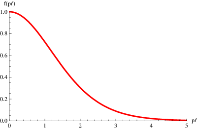
The full answer is a the 4d GGM [42] answer multiplied by a momentum dependent form factor
| (2.36) |
plotted in figure 2.2. We may recover the four dimensional limit , where
| (2.37) |
Subleading contributions
In this section we would like to discuss the subleading contribution to sfermion masses () pictured in figure 1.3 (See also [61, 60, 67]). In the all order kk model [1] its contribution is given by
| (2.38) |
In general, this integral is divergent due to the brane to same brane propagator on the hidden brane that connects the double mass insertions. The four dimensional limit, when i.e. is small one finds
| (2.39) |
In the limit one may carry out a Matsubara summation and finds
| (2.40) |
where in this limit
| (2.41) |
The integral is IR divergent and must be regulated. We choose
| (2.42) |
| (2.43) |
Schematically, for a messenger sector, one can compare the leading order and subleading contribution
| (2.44) |
such that it is not always clear which term is truly leading order. is the four dimensional scalar mass scale and is the gaugino mass scale. When comparing versus may be sufficient, however models with an approximate R-symmetry may also suppress . It is worth emphasising that for the generalised messenger sector discussed in this paper and for typical values of , and when , the double mass insertion in figure 1.3 is most likely to be the largest contribution to sfermion masses, however for ISS-like models [1, 65] where the gaugino mass is suppressed due to an R-symmetry, figure 1.2 is the leading contribution. We also stress that it is completely reasonable to build models whereby , in which case this model is in a Hybrid regime where both digrams will play significant roles in the contribution of soft masses to scalars, for example in chapter 5. It is also useful to note that the subleading diagram may act as a bound, at the high scale , on the ratio of masses:
| (2.45) |
where in the last line we took =0.04.
2.2.3 Hypermultiplet scalar masses
The supersymmetry breaking masses of the bulk hypermultiplet scalars and hypermultiplet fermions can also be computed in the gauge mediation setup and couple to the hidden brane exclusively via , when using the action Eqn. (2.7). The diagrams for the scalars are similar to those of Figure 1, but include an additional contribution with a bulk propagator, indicated with the symbol, coupling the positive parity gaugino to the negative parity bulk fermion
| (2.46) |
A similiarly constructed propagator can be written in the and basis for the 5D wavefunction.

To compute the diagrams: The current correlators (blobs) are brane localised, however the vertices joining the vector fields to the hyperscalar must be integrated over all of . One must also specify the 5d wavefunction ( momenta) of the external hyperscalar legs using
| (2.47) |
at the sewing point , which is then integrated over. The second diagram does not contribute to the mass due to transversality. The rectangle in the final diagram represents that the diagram is completely localised on the hidden sector brane, including the vertices that couple to the external hyperscalar legs.
We will focus on the zero mode mass ()
| (2.48) |
where
| (2.49) |
| (2.50) |
The momentum integral is UV divergent. Physically this is to be expected as the hypermultiplet is not brane localised and so unlike the sfermion masses there is no brane separation to suppress large momenta contributions. We can extract the dependent susy breaking mass [68]. We take where
| (2.51) |
2.2.4 Vacuum Energy
The propagation of supersymmetry breaking effects in the bulk produces a non zero vacuum energy. The computation of the vacuum diagrams at the order is similar to the scalar masses in the previous sections. Similarly to the computation of the hypermultiplet scalar masses, the diagram with and that with combine and yield a contribution proportional to . By including all other diagrams we obtain
| (2.52) |
is the dimension of the adjoint representation of the gauge group . The vacuum energy is also UV divergent. The Casimir energy is the component of the vacuum energy where the bulk propagation winds . This, in general, will contribute to the determination of the physical value of , along with other supergravity corrections. The Casimir energy is given by
| (2.53) |
2.2.5 Semi-Direct Gauge Mediation via the bulk
In [50] semi-direct gauge mediation in a setup is explored using current correlators. In this section we comment on the semi-direct case in our setup with two Branes and a bulk. One brane is the MSSM brane, described by some generic chiral matter, charged under the visible gauge group , which lives in the bulk. The other brane is a SUSY breaking brane. The messenger fields are located on this brane and are charged under both and a brane localised gauge group . The messengers do not participate directly in the susy breaking dynamics, however they couple to the brane localised susy breaking sector via gauge interactions with gauge group and by construction the messengers and susy breaking sector decouple as .
The Gaugino masses vanish at leading order (three loops) precisely because of the argument of [50]. The sfermion masses in a flat bulk are found to be
| (2.1) |
where
| (2.2) |
is the mass of the messengers. are the kernels, which in principle could be different for each of . In [50], it was checked that , so we will ignore this supscript index.
As a final comment, one motivation for GGM5D is that it makes the partitioning of the hidden and visible sector a geometric feature. One may be motivated to make semi-direct mediation a geometric feature too by placing the SUSY breaking sector , the messengers and the MSSM on three distinct branes. It would be interesting to study explicitly if it is possible to realise such a possibility in a concrete model.
2.3 Generalised Messenger sector
In this section we give a concrete description of the 4-dimensional susy breaking brane and consider two sets of chiral messenger coupled to a spurion field . We follow [71] and extend the usual setup of a generalised messenger sector to the case where the gauge multiplet propagates in a 5d orbifold.
The superpotential describing the coupling of the messengers and the spurion is identical to that considered in [71] and is localised in the fifth dimension on the susy breaking brane
| (2.1) |
where and are generic matrices. We assume that all chiral fields have canonical kinetic term and so, after a field redefinition, we can take to be diagonal with real eigenvalues , where, as usual, is the vev of the scalar component of the spurion superfield . Further, we take to be hermitian and by using unitary matrices one may diagonalise the bosonic mass-squared matrix
| (2.2) |
Such that has real eigenvalues . We define two mixing matrices:
| (2.3) |
The calculations are carried out explicitly in section D; in this section we simply display the results.
2.3.1 Gaugino masses
As we have seen in the previous section, the Majorana gaugino mass matrix of the 5d model couples every Kaluza-Klein mode to every other with the same coefficient and this contribution is captured in (2.28). In this case we can compute explicitly the correlator determining by using (D.1.4)
| (2.4) |
are messenger indices running from to , the number of messengers, while is nonzero and equal to or only if and are in the same representation. In the full mass matrix one must take into account the Dirac masses of the Kaluza-Klein tower itself. However, the susy breaking contribution Eqn. (2.4) is identical to the purely 4-dimensional case and it is possible to follow [71] for various case by case simplifications. For instance, when , to lowest order in and for fundamentals one finds
| (2.5) |
which is a familiar result.
2.3.2 Sfermion masses
The sfermion masses are sensitive to the extra dimension . In the small limit the 4d results are recovered and this is fully explored in [71].
Large
When is smaller than the scales and the sfermions masses can be written as
| (2.6) |
are the quadratic Casimirs of in the gauge group . The sfermion scale is22 2 See Appendix D for its derivation.
| (2.7) | |||||
We may reduce to minimal gauge mediation [72] by setting in equation (2.1)
| (2.8) |
| (2.9) |
| (2.10) |
for can be reasonably approximated by and are the eigenvalues of in (2.1).

The limit of small multi-messenger mixing effects gives
| (2.11) |
In the limit, and small multi messenger mixing, we would like to derive the analog sfermion formula found in [73]. The additional factors cannot be taken inside such that we find
| (2.12) |
Where are in this case the complex eigenvalues of .
Intermediate
In the intermediate limit that , the large results are still valid and . Reducing to minimal gauge mediation () we find
| (2.13) |
The limit of small multi-messenger mixing effects gives
| (2.14) |
Finally we comment on the ratio . In “(Extra) Ordinary Gauge Mediation” [73], this quantity is defined as and it may vary continously between and , the number of messengers. This definition is peculiar to the 4d models; we may easily have and in this 5D construction. To avoid confusion we will refer to it as a ratio and not as .
2.3.3 Hyperscalar zero mode mass
The positive parity scalar of the hypermultiplet have a susy breaking mass term. In this paper we compute only the zero mode scalar. We may use the same expansions of the function in square brackets (Appendix D.1.1) we used for the sfermion masses. In general we can define
| (2.15) |
is the Casimir of the representation of the positive parity hypermultiplet . We now look at the various limits.
Small
Large
When is smaller than the scales and we may start from Eqn. (2.51). We know that the function in square brackets is independent of and can be found in appendix D.1.1, so we may evaluate the dependent integral independently. The result is
| (2.18) |
is written explicitly in the previous subsection. The intermediate limit can be found by setting . The zero mode fermions of the hypermultiplet receive no susy breaking mass corrections at order .
2.3.4 Casmir Energy
The Casimir energy can be computed for the generalised messenger sector just as for the sfermion and hyperscalar zero mode mass by using the results of appendix D. In particular using Eqn. (2.53) and restricting to the case of minimal gauge mediation and for a single set of fundamental messengers we find
| (2.19) |
This result reproduces exactly the result of [56].
2.4 Chapter Summary
We have computed bulk gauge mediated supersymmetry breaking of supersymmetry from a hidden to a visible brane, using the current correlator techniques of [42]. We obtained analytic results for both semi-direct and direct coupling of the messengers and susy breaking sector, located on a hidden brane.
To summarise, we have found that there are two limits, one in which the leading order scalar masses are four dimensional and one in which kk modes are lighter than the scale , in which case we have found the leading order scalar masses are screened. Overall we have shown that the lightest gaugino mass is unaffected by the extra dimension. We would like to emphasise one point, the RGE equation for scalar masses in the five dimensional limit will differ from the four dimensional RG equation there will be many more gaugino masses.
In the next chapter will demonstrate how the framework so far constructed, may be applied to model building using Seiberg duality and in particular metastable supersymmetry breaking models of the ISS type.
Chapter 3 Dynamical Supersymmetry breaking: ISS on the brane
A particularly popular and natural form of gauge mediated supersymmetry breaking is the construction of ISS [24]. In ISS, supersymmetry is broken non-perturbatively in the electric description and is metastable. It is a simple SQCD model and as a result one may apply Seiberg duality to obtain an effective magnetic description in which supersymmetry breaking can be explored perturbatively. It is well known that this theory has a signature of light gauginos relative to heavier sfermions and this is seen as an unfortunate drawback.
In this section we turn to an explicit application of 5D general gauge mediation which will alleviate the above mentioned problem by screening the leading order scalars masses. We construct a scenario in which the ISS model [24, 74] is located on the hidden brane. We choose to explore supersymmetry perturbatively in the macroscopic (magnetic) variables in the window . We have an SQCD with magnetic gauge group and flavours where . The superpotential is
| (3.1) |
The magnetic meson is a gauge singlet and an adjoint of the flavour group. The magnetic quarks and are fundamental (antifundamental) of the gauge group and antifundamental (fundamental) of the flavour group, respectively. Supersymmetry is broken by rank condition when , as only the first F terms of can be set to zero. Following the model explored in [75, 76, 77, 5], the matrix is explicitly broken
| (3.2) |
with , and additionally we include the deformation
| (3.3) |
As mentioned mentioned more fully in [75, 76, 77, 5], this deformation explicitly breaks R-symmetry thus allowing gaugino masses. The final unbroken vacuum symmetry groups and matter content is
| Field | ||
|---|---|---|
Where arose from the magnetic “colour flavour locking” of . The superpotential is
| (3.4) |
We have two choices of embeddings: we choose to weakly gauge either of the flavour symmetry groups or and associate it with the gauge group in the bulk. One may choose for simplicity an standard model “parent” gauge group. The messengers of this model are the ’s and ’s in either embedding. Additionally for the embedding of the degrees of freedom of may also contribute as messengers as has been explored in [5]. The other fields do not contribute as messengers. We take these fields to have a canonical Kähler potential and all the matter on the MSSM brane to have a canonical Kähler potential coupled to this bulk gauge superfield. Classically the potential is
| (3.5) |
singlet is the Goldstino superfield and the scalar component is a classical modulus and its vacuum expectation value, is found by minimising
| (3.6) |
where is the corresponding Coleman-Weinberg potential
| (3.7) |
The Casimir energy is sufficiently suppressed to be ignored at this stage. We find
| (3.8) |
where we have expanded to first order in and in up to first non-vanishing order [5]. We have suppressed factors of in the expression for coming from tracing over degenerate mass eigenavalues.
3.1 Large mediation
The susy breaking contribution to the gaugino masses are
| (3.9) |
where are the eigenvalues of the fermion mass matrix of messengers derivable from Eqn. (3.4) and computed in [76, 5]. The messenger sector is dominantly in both embeddings of the standard model and we find the susy breaking mass to be
| (3.10) |
As we have highlighted throughout, the mass eigenstates must be found after inclusion of the kk masses, to the mass matrix. The sfermion masses can be found, using the results of the previous section, from
| (3.11) |
with
| (3.12) |
We find
| (3.13) | |||||
Which is non-zero but highly suppressed.
3.2 Intermediate mediation
In the intermediate range that the vacuum energy is given by Eqn. (2.19), with This time, however, the zero mode gaugino mass can be approximated by Eqn. (3.9):
| (3.14) |
and there is no problem of kk mixing. The sfermion masses are still given by Eqn. (3.12). As a first approximation, one may ignore this contribution to sfermion masses entirely. One then lets the renormalisation group flow at the high scale down to the low scale generate sufficiently heavy sfermions to avoid current bounds.
3.3 The Emergent Lattice
In the previous section we placed the ISS model on the fixed point of the extra dimension and the theory is truly five dimensional. In this section we will demonstrate how an effective extra dimension may emerge in the magnetic description of certain classes of SQCD theories and will motivate a lattice (de)construction of the general gauge mediation formalism.
First a crucial comment is necessary. Under Seiberg duality global symmetries are preserved. This must be so as global symmetries are associated with observable currents and so must be the same under the duality. The gauge symmetries on the other hand, are a redundancy in the description. One may ask how it is possible that two theories may have differing number of gauge bosons and gauginos. Importantly the two theories are at a scale invariant fixed point, where there are no asympotically free states and no well defined particle interpretation. We can of course deform the model by adding quark masses to the electric description and now particle states are well defined and the duality becomes an effective one. In fact it is curious to ask what becomes of the gauge bosons of the magnetic group? The answer lies in that the dual of the quark mass matrix completely Higgs’ the magnetic gauge group and those degrees of freedom become vector mesons. As a result in terms of the low energy effective description the gauge fields are now observable as vector mesons.
A further insight is necessary. If we weakly gauge a global symmetry, then additional massless vector fields arise which are not related to the Seiberg duality. One can think of these fields as external “probes” of the SQCD theory. However, if the magnetic group, or some subgroup of this, undergoes a “magnetic colour-flavour locking” with the weakly gauged global symmetry, then the vector fields will appear to have massless modes and Kaluza-Klein modes from the vector mesons: a deconstructed extra dimension emerges. From the perspective of the electric description, resonances have filled the first level of a Kaluza-Klein tower on top of the massless external fields. From the perspective of the magnetic description, this can be seen to take place dynamically as the system undergoes the locking.
The remainder of this chapter is essentially a review of [65], which demonstrates how the locking arises dynamically, which we feel is crucial in developing many of the concepts in the remainder of this thesis and as a building block in the AdS/CFT construction of chapter 6.
In [65] An electric SQCD hidden sector was chosen
| Field | ||||
|---|---|---|---|---|
| 1 | ||||
| -1 | ||||
| 1 | -1 | |||
| 1 | 1 |
where the indices and , with the superpotential
| (3.15) |
The factor of the previous section has been set to one for simplicity. The flavour symmetires may be thought of as arising from after the introduction of the quark mass term, which is then further broken to after the introduction of the operators. The flavour symmetry preserving masses are .
In the window , this theory flows to an IR free magnetric Seiberg dual description with gauge group and UV cutoff . The superpotential is given by
| (3.16) |
The representations of the magnetic description are given by
| Field | |||
|---|---|---|---|
| 1 | |||
| 1 |
where we have chosen subscript labellings of the groups to make clearer the patterns of breaking. After integrating out the heavy states using the equations of motion of the ’s, one obtains
| (3.17) |
where . The theory now has two sectors which in principle decouple when but more importantly the MSSM completely decouples when
Next, we proceed to explore the vacuum symmetries of the theory. If we choose for simplicity then we see that all ’s are will be Higgsed as that F terms of can all be set to zero:
| (3.18) |
Using the remaining symmetries, one may further diagonalise the ’s to the vacuum
| (3.19) |
Crucially, these fields will play the role of linking chiral superfields in a deconstructed model and they link the lattice site with the flavour site.
In the second sector has maximum rank however the matrix has rank . For supersymmetry is broken by rank condition as only the first F terms may be set to zero. Hence the global symmetries will break further from and one finds
| Field | |||
|---|---|---|---|
where , , . As the flavour symmetries are broken we may choose different masses identify as the unhiggsed part of the original masses. The classical vacuum is now given by
| (3.20) |
The singlet is the Goldstino superfield of spontaneous supersymmetry breaking. As the fermionic component is a massless Goldstino, the scalar is a pseudomodulus. The supersymmetry breaking sector has the symmetry groups times the unaltered flavour group . The supersymmetry breaking sector has an approximate R-symmetry and one may choose different deformations such as the demonstrated in the previous section. The sector of messengers and supersymmetry breaking field has a similar structure to the one analysed in the previous section, althought the rank conditions arise differently. In this model the flavour group must be weakly gauged and associated with the standard model. This weakly gauged group then shares properties with the visible sector fixed point of the previous model. Similarly the hidden brane is equivalent to the lattice site. As discussed before, this model is crucial for developing a dynamical description of how a system undergoes the “magnetic colour-flavour locking” and vector mesons fill up as kk modes above the massless external “probe” gauge fields of the weakly gauged global symmetry. This strongly motivates the AdS/CFT construction of chapter 6 whereby a weakly gauged global symmetry of the UV CFT description arises as a gauge symmetry in the bulk AdS description.
Many questions still remain. It would be very interesting to see if one can populate more levels of the Kaluza-Klein tower dynamically using Seiberg duality and finally arise at a contintum limit of AdS space, perhaps starting from the conformal window with large . This also strongly motivates a study of observing these kk modes at the LHC and furthermore by interpreting them as resonances of a strongly coupled hidden sector, extract from them properties of the hidden sector, such as their internal degrees of freedom as UV quarks, and their quantum numbers under the UV gauge group. Some work in this direction has already been completed [78, 79, 80].
Chapter 4 General Gauge Mediation and Deconstruction
In this chapter we locate a supersymmetry breaking hidden sector and supersymmetric standard model on different lattice points of a quiver gauge diagram [81, 82, 83, 84, 85, 86, 87]. The hidden sector is encoded in a set of current correlators and the effects of the current correlators are mediated by the lattice site gauge groups with “lattice hopping” functions and through the bifundamental matter that links the lattice sites together. We show how the gaugino mass, scalar mass and Casimir energy of the lattice can be computed for a general set of current correlators and then give specific formulas when the hidden sector is specified to be a generalised messenger sector. The results reproduce the effect of five dimensional gauge mediation of chapter 2 from a purely four dimensional construction [67].
In this construction each lattice site is a copy of a four dimensional supersymmetric standard model parent gauge group . Each lattice site is connected using bifundamental chiral superfields that link the lattice together. The combination of super Yang-Mills with specified “lattice hopping” vectors and the bifundamental linking matter, will mediate the supersymmetry breaking effects from the hidden sector lattice site to the standard model lattice site, to generate sfermion masses [67, 88]. In this model, the lattice site spacing will be the scale that suppresses the momentum in the loops for sfermion masses. We shall see that effective five dimensional suppression effects arise when and that we recover four dimensional effects when . At low energies this lattice construction is equivalent to the five dimensional orbifold model mentioned above. The scale arises in the masses of the propagating gauge fields and bifundamental matter which resemble KK states at low energies. The masses of the KK spectrum are generated by the vacuum expectation value of the scalars of the bifundamental chiral superfields that link the lattice together and so we see that these suppression methods are all related.
4.1 Framework
This section concisely reviews the construction of the orbifold moose (quiver gauge diagram) following the work of [67]. We start with a lattice of four dimensional, super Yang-Mills gauge groups all identified with the gauge groups of the supersymmetric standard model. The matter content of the lattice is:
The are bifundamental chiral superfields that link the lattice sites together. The are gauge indices labelling the fundamental or antifundamental of the gauge group . The bifundamental scalars all obtain a vacuum expectation value , which may be generated by some dynamical superpotential [82, 67]. The indices label the lattice, running from to (mod ) with lattice spacing , such that is the length of the lattice. The five chiral multiplets and five are localised on the endpoint lattice sites and are required to cancel anomalies due to the breaking of “hopping” symmetry at the lattice end points. These are inessential to the discussion of gauge mediation. The and play the role of the standard model matter and Higgs superfields. Additionally, we may add the fields as messenger superfields coupled to a spurion . These fields will enter the discussion when we specify a generalised hidden sector in a later section.
The bifundamental scalars are given a vacuum expectation value and fluctuations about that value, . The scalar kinetic terms of the bifundamental matter are used to generate a mass matrix for the gauge bosons, via the Higgs mechanism. The mass spectrum is computed in [67] and in [82, 81, 84]. For the gauge bosons, the masses are
| (4.1) |
A key attribute of this setup is that lattice eigenstates are not mass eigenstates of the system. The mass eigenstates are given by
| (4.2) |
These are even parity modes. The fermion mass matrix of bifundamental fermions and gauginos must be diagonalised as in [67]. The even states have masses
| (4.3) |
and eigenvectors
| (4.4) |
The odd parity fermions have masses
| (4.5) |
with eigenstates
| (4.6) |
In the continuum limit, the fermions should coincide with the adjoint fermion of a negative parity chiral superfield. To construct this adjoint fermion one identifies the bifundamental scalar with the unitary link variable: where is a unitary matrix. Keeping track of indices we may relabel , where both indices are valued at the ’th lattice site. A negative parity adjoint scalar is similarly defined and as the multiplet is supersymmetric, the mass spectrum and eigenstates are equivalent to that of the fermion.
Using the above eigenfunctions, the mixed space scalar propagator can readily be determined by insertion of a closure relation for the mass eigenstates. The result is
| (4.7) |
In summary, the resulting low energy degrees of freedom and field content for large is that of an positive parity vector multiplet and negative parity chiral superfield of super Yang-Mills in five dimensions compactified on [66, 1].
4.1.1 The periodic lattice
It is useful to compare this construction with that of a periodic lattice corresponding to a theory compactified on a circle [67]. The anomaly cancelling and fields are unwanted in the periodic construction. All the bulk fields have a mass spectrum given by
| (4.8) |
The vector superfield mass eigenstates are also related to the lattice eigenstates through
| (4.9) |
The mixed space scalar propagator for the circle may also be written as
| (4.10) |
The low energy degrees of freedom are of a full model, including restoring the zero modes that had been projected out by negative parity, in the interval case.
4.2 Lattice localised currents
This section will encode a SUSY breaking sector, localised on the lattice site i=0 in terms of current correlators [42]. The lattice has a set of vector superfields and a set of current multiplets associated to the bifundamental matter linking the lattice11 1 In this discussion we will ignore the currents of the fields and .. The supersymmetric standard model matter (visible sector) will form a current multiplet . Additionally, we may locate a hidden sector at lattice point , .
We may couple the hidden sector current multiplet to the lattice gauge fields
| (4.1) |
As this whole discussion refers to the hidden sector current multiplet at , we will drop the hidden sector index. The change of the effective Lagrangian on the i=0 lattice site to is
In the next subsections we will use this effective action to determine soft mass formulas and the Casimir energy of the lattice.
4.2.1 Gaugino masses
A soft supersymmetry breaking gaugino mass for the lattice sites arises at tree level. It is given by
| (4.2) |
In the continuum orbifold scenario [1], the orbifold fixed points break Lorentz invariance in the fifth dimension and this is signified by the ‘‘brane’’22 2 The word “brane” being used to denote the ends of an interval, where matter is located in five dimensional orbifold constructions. localised current correlators not preserving incoming and outgoing momenta. These current correlators therefore couple, equally, to all states of the K.K. tower of vector superfields. In the lattice picture the currents only coupled to fields at a single lattice site. However it is precisely because the lattice fields are a sum of mass eigenstates, that the current correlator still generates a correction to all mass eigenstates in the lattice picture. The soft term mass must be included in the full mass matrix of all fermions () in the lattice and if we assume that is small, we may treat this as a perturbation of the full mass matrix. This process is outlined in [67] and one finds the zero mode mass is
| (4.3) |
The four dimensional coupling is determined from . The mass splittings are also similarly obtained
| (4.4) |
Heuristically, we see that it is the process of moving from lattice states to mass eigenstates that reproduces the orbifold effect of a soft mass coupling to all K.K. modes.
4.2.2 Sfermion masses

We would like to propagate the effects of supersymmetry breaking from the lattice site to the site to generate scalar masses for the MSSM located at that site. This is a loop diagram with intermediate gauge boson, gaugino and term as can be seen in figure 4.1. The gauge boson and gaugino are dynamical and they may propagate around the lattice using the “lattice hopping” wavefunction. The lattice scalar propagator Eqn. (4.7) from the hidden sector lattice site to visible lattice site is
| (4.5) |
For the periodic lattic case the same final equation holds, after adjusting for the mass eigenstates by in the denominator. We highlight that from interval to interval fixed point propagators, the factor arises. This factor is crucial in the cancellation of alternate states of the K.K. tower which generates the suppression of sfermion masses at large momenta and keeps “brane to brane” diagrams UV finite. This factor does not arise in “brane” to same “brane” diagrams, which is why the vacuum energy diagram is divergent. Equally, diagrams with a double insertion of the gaugino mass will also be UV divergent. To generate a gaugino or gauge boson propagator we supplement this scalar propagator with the correct Lorentz structure of a fermion, or transverse gauge projector as necessary. The remaining diagram propagated by , is not so simple. In orbifold models [1], the term is given by , where is a dynamical negative parity scalar field and is a derivative in the fifth direction. This field contributes to the propagation of supersymmetry across the interval. To make the dynamical on the lattice, one may integrate out this auxiliary field in terms of the lattice currents and find
| (4.6) |
The index is a generator index running from to . Next, using where is a unitary matrix and keeping track of the indices of each gauge group one finds
| (4.7) |
where we have relabelled . The contraction of indices has resulted in an adjoint scalar of the ’th lattice site and both indices are valued at the same lattice site. In the continuum limit, the term is a lattice derivative of [89]:
| (4.8) |
We may now associate with the negative parity scalar of the super Yang-Mills action. An additional manipulation used to calculate this diagram in orbifold models, is to use
| (4.9) |
to exchange terms, generated by the derivative , for . Whilst this manipulation is rather less precise on the lattice than in the continuum limit, it is necessary to ensure that corrections to the beta function due to a supersymmetric hidden sector cannot generate sfermion masses. Collecting the contributions from all three diagrams, the sfermion formula is
| (4.10) |
where
| (4.11) |
For the interval model, using Eqn. (4.7) gives
| (4.12) |
The same equation holds in the periodic case, using the periodic mass eigenstates . In this equation, we have used a standard model lattice with gauge coupling where refering to the group respectively. is the quadratic Casimir of the representation of the scalar mass in question, under the gauge group . The integral is UV and IR finite. As discussed in the introduction, one can see that the momentum integral in this equation will be suppressed by the product of KK propagators with length scale entering from the mass of the KK modes. The limit in which there is a single lattice site () is the corresponding four dimensional limit. We find
| (4.13) |
This equation reproduces exactly the result of “General gauge mediation” [42]. For lattice sites, we may take the two gauge eigenmasses to be and . For the sfermion mass formula, one obtains
| (4.14) |
where the unwanted factor of is absorbed into the gauge coupling .
4.2.3 The Casimir energy
In a globally supersymmetric theory the vacuum energy is zero. Supersymmetry breaking effects of the hidden sector will generate a vacuum energy and the lattice dependent part of this vacuum energy will correspond, in the continuum limit, to the Casimir energy of a higher dimensional theory [89, 56, 1]. To calculate the Casimir energy we must compute the vacuum diagrams that appear in figure 2 of [45]. Each vacuum diagram may be generated by simply forming a closed loop with the field that propagates each current correlator in the effective action. The propagation is from the zeroth lattice site back to the zeroth lattice site in the loop. The zero to zero lattice site propagator is given by
| (4.15) |
This time there is no product form for the propagator as the is absent. The vacuum energy is given by
| (4.16) |
is the dimension of the adjoint representation of the gauge group . This integral is UV divergent. To extract from this the finite Casimir energy, one must extract the continuum limit of this sum. The prescription for this is found in [89]. Additionally, the appendix includes relevant steps which are applied in the next section, where we focus on a generalised messenger sector for which the terms may be determined.
4.3 Generalised messenger sector
In this section we give a concrete description of matter content of the SUSY breaking sector located at the zeroth lattice site, following the construction of [72]. We consider sets of chiral superfield messengers33 3 We hope that this index which runs to , the number of messengers, does not get confused with the lattice site index of the previous section. in the vector like representation of the lattice gauge group, coupled to a SUSY breaking spurion with . Generalisations to arbitrary hidden sectors are a straightforward application of the results of [71, 1]. The superpotential is
| (4.1) |
In principle is a generic matrix which may be diagonalised to its eigenvalues [72]. The messengers will couple to the bulk vector superfield as
| (4.2) |
We can extract the multiplet of currents from the kinetic terms in the above Lagrangian. The current correlators can then be computed and their results can be found in [42, 1, 71]. We will use the result of these current correlators to determine the gaugino massses, sfermion masses and Casimir energy.
4.3.1 Gaugino masses
The SUSY breaking zero mode Majorana gaugino mass is found by first evaluating the current correlator in Eqn. (4.2), which may be found in [72, 42, 1], and then diagonalising the full fermion mass matrix and extracting the zero mode as discussed in the previous section. For the zero mode this simply fixes . The zero mode gaugino mass is found to be
| (4.3) |
The label refers to the gauge groups , is the Dynkin index of the representation of and
| (4.4) |
where . for small [72].
4.3.2 Sfermion masses
The entirely four dimensional limit of the sfermion mass formula when both the hidden and visible sector are located on the same single lattice site, is displayed in Eqn. (4.13). For the generalised messenger sector, this four dimensional result can be found in [72]. To obtain an effective five dimensional behaviour from the lattice, one must require sufficient lattice sites to suppress large contributions to loop momenta in the diagrams contributing to sfermion masses. We start with Eqn. (4.12) and when , one may then expand the current correlators in the limit and find [1]
| (4.5) |
which is independent of at this order. The function is given by
| (4.6) |
where for can be reasonably approximated by . We find
| (4.7) |
where
| (4.8) |
and is an integral that depends on the number of lattice sites
| (4.9) |
The function behaves like
| c | ||||
|---|---|---|---|---|
| 0. | 25 | 0.0625 | 4 | |
| 0. | 029 | 0.012 | 2.4 | |
| 0. | 0082 | 0.0039 | 2.1 | |
| 0. | 0032 | 0.0016 | 2 | |
| 0. | 0015 | 0.00077 | 2 | |
| 0. | 00079 | 0.00042 | 1.7 | |
Rescaling and taking we find that the sfermion mass scales as
| (4.10) |
which reproduces the results of the Mirabelli-Peskin model [56, 1].
4.3.3 Casimir energy
The Casimir energy of the lattice can be extracted from the vacuum energy by taking the difference between the lattice propagator and its continuum counterpart. This will cancel the divergent parts of the momentum integral in the vacuum energy. The final answer will be an approximate result that approaches the continuum Casimir energy when the number of lattice sites is infinite. We start with Eqn. (4.16). The sum of terms is still given by Eqn. (4.5). We then must solve the UV divergent momentum integral in Eqn. (4.16):
| (4.11) |
Next we take the difference between the lattice and continuum momentum integral as
| (4.12) |
The divergent parts of the lattice and continuum limit of this function will cancel out, leaving the finite mass dependent parts. Additional steps may be found in the appendix which follow the procedure of [89]. The renormalized function is given by
| (4.13) | ||||
| (4.14) |
where
| (4.15) |
In the continuum limit is
| (4.16) |
For the Casimir energy, we obtain
| (4.17) |
This result agrees with the Casimir energy found in the Mirabelli-Peskin model [56] when . The Casimir energy for the periodic case is similarly obtained
4.4 Summary and conclusion
In this chapter we combined the framework of encoding generic hidden sector in terms of current correlators [42], with the four dimensional construction of supersymmetric extra dimensions on a lattice [67]. This extends previous lattice constructions of supersymmetry breaking so that different hidden sectors may be explored. We have demonstrated that the low energy description of this model matches that of extra dimensional supersymmetry breaking on an interval [1]. In particular we have shown that when the scale of the lattice is much smaller than the characteristic scale of the hidden sector , then for a perturbative messenger sector sfermion masses are suppressed by an additional factor relative to pure four dimensional gauge mediation. This suppression arises due to the suppression of momenta in the outer loop of the two loop diagrams generating sfermion masses.
It is useful to note that the running gauge coupling for a “flat” lattice has been explored in [90, 91, 92]. Also various related such as an open moose [39] have been shown to have similar features to that of the AdS/CFT correspondence which is a topic we will return to in chapter 6.
In the next chapter we will look at a special case of five dimensional gauge mediation in which there is only 1 massive kk mode of the vector superfield assisting in the mediation of the breaking effects. This special case is equivalent to the two lattice site model mentioned earlier in this chapter. We will find that due to special properties of two loop feynman diagrams, the leading order scalar soft masses of the two site lattice model may be analytically determined for all ratios of the lattice spacing versus and a new hybrid regime is uncovered.
Chapter 5 Hybrid Gauge Mediation
In this chapter we would like to examine a particular effective model in which the vector superfield that mediates supersymmetry breaking has only a massless zero mode and one Kaluza-Klein mode with mass . This model is particularly interesting for two principal reasons. First the model arises quite naturally as the minimal case of a deconstructed lattice of chapter 4 and as an effective model of a flat extra dimension as in chapter 2. Secondly this model not only captures all the essential features of both the gauge and gaugino mediated limits, it also allows one to interpolate between these limits analytically and explore a new hybrid limit. This hybrid regime is rather new and we hope it receives further attention.
To understand this model we will recapitulate some of the key features of general gauge mediation in five dimensions: In gauge mediated supersymmetry breaking, one may broadly split models into two classes, those that are gauge mediated and those that are RG gaugino mediated. Let us clarify further: using the construction of general gauge mediation found in chapter 2, the soft term for scalars masses at lowest order in is dependent on a super-traced set of current correlators
| (5.1) |
as pictured in figure 1.2. In general, given a perturbative hidden sector, we may expand this set of current correlators in either of two limits to obtain analytic expressions: the four dimensional gauge mediated limit or the screened (five dimensional) limit [56, 1, 3, 2]. In this second limit the scalar soft masses are rather suppressed at the high characteristic scale of the hidden sector. However, due to the gaugino mass contributions in the renormalisation group equations (RGE’s)11 1 See [57, 58, 59] for the four dimensional RG equations. [93] as in figure 1.3, scalars develop soft masses at low scales through RG gaugino mediation [62, 63]. We should of course point out the mechanism by which one discriminates between the two expansion limits: when a mass scale enters into the outer loop (see figure 1.2) of the leading order sfermion mass diagrams with , this mass scale suppresses loop momenta and warrants expanding the current correlators in the screened limit. As higher dimensional models naturally introduce this mass scale through Kaluza-Klein (kk) modes, it is customary that the screened limit become synonymous with higher dimensional mediation of supersymmetry breaking.
It is natural to ask if there is some intermediate type of mediation whereby the leading order scalar soft masses are still somewhat suppressed at the high scale but not as drastically as in gaugino mediation limit, such that both the leading order contributions and subleading RG contributions play a significant role: hybrid gauge mediation. The hybrid regime, when , cannot be accessed by expanding the current correlators in and one must find a new way to evaluate the sfermion diagrams. However for the case of a minimally truncated kk tower with just one massive kk mode, the leading orders sfermion diagrams are analytically solvable for all ratios of , and and one can not only interpolate between the four dimensional and screened five dimensional limit, but one can also access the hybrid regime.
The key message of this chapter is that whereas gaugino mediated models typically give a leading order sfermion mass of
| (5.2) |
more generally by changing the ratio of the first kk mass with one can obtain analytic formulas whereby
| (5.3) |
where takes real values between and .
The hybrid regime has been explored for a (de)construction model [94, 95]. It also naturally arises in ISS-like models that exhibit magnetic colour-flavour locking that generate linking fields which we focused on in chapter 3. Phenomenological scans which implement hybrid gauge mediation have also already been explored to some degree [96, 97, 98, 99] by virtue of having a nonzero scalar soft mass at a high scale and effective four dimensional RG equations when . In this chapter we will obtain completely analytic solutions for the leading two loop scalar soft masses and highlight the hybrid regime. We will do this predominantly for the five dimensional model of chapter 2 although we also highlight the usefulness of these results to the (de)construction model as first pointed out in [94, 95].
5.1 The minimally truncated model
We saw in chapter 2 that all the kk modes of the vector superfield, in principle, propagate the supersymmetry breaking effects from the hidden to the visible brane. If the mass scales of the model are sufficiently separated, we are at liberty to analyse an effective model in which only the zero mode and first mode of the kk tower with mass of vector superfields are part of the spectrum by placing a cutoff above these scales, as depicted in figure 5.1. As any finite truncation of kk modes in the vector superfield may be related in the IR to a finite lattice (de)construction model [3, 67], the results of this minimal truncation can be related to the minimal (de)construction model explored in [94, 95, 100].

5.1.1 Gaugino soft masses
We start by highlighting the 4 leading soft gaugino mass contributions which are given by
| (5.4) |
Due to these soft masses, when computing the RG gaugino mediated contributions (as in figure 1.3) above the mass scale this will require evaluating the RG contributions from 6 diagrams. When running RG equations at energy scales below , only the diagram built from contribute and the four dimensional RGE’s are sufficient.
5.1.2 Sfermion masses
Supersymmetry breaking effects encoded on the hidden brane are mediated to the visible brane by both modes . One may write the brane localised sfermion mass summations of Eqn. (2.33) as a product. After a Wick rotation one finds22 2 We have rescaled the factors of into the coupling
| (5.5) |
with
| (5.6) |
The form factor is plotted in figure 5.2 and captures the essential screening behaviour of the all order model plotted in figure 2.2. This result has also been obtained for the (de)constructed version of this model [100].
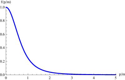
5.1.3 Bulk scalar masses
In [1] the positive parity bulk hyperscalar zero mode masses were computed. For the two state model it is given by
| (5.7) |
where
| (5.8) |
This can be rewritten as (we Wick rotated and then manipulated)
| (5.9) |
We will show in section 5.2 how this soft mass may be analytically determined for a specific hidden sector and specified currents. In the next section we will show that this mass formula will determine the soft masses of linking fields in the minimal gaugino mediation model.
5.1.4 Minimal gaugino mediation: Linking scalar soft masses

The minimally truncated five dimensional model we have been describing so far can be related, in the IR, to the minimal gaugino mediation model pictured in figure 5.3. This means that the soft masses written above may be also be used for this lattice model. This has been shown to be the case in [94, 100, 95]. In this section we would like to briefly comment on this model by showing how the linking scalar soft masses also match that of the positive parity hyperscalar mass formula Eqn. (5.8).
The kinetic terms for the bifundamental chiral superfields of the minimal model are given by
| (5.10) |
where for simplicity we have taken . We see that for the minimal model of figure 5.3 the linking fields will each pick up two leading order soft masses, being bifundamental. The resulting soft mass for is given by where
| (5.11) |
| (5.12) |
Adding these contributions, one obtains the hyperscalar mass result Eqn. (5.8) and emphasises the similarity between lattice and continuum models. The mass eigenstates are then given by the full mass matrix including the kk masses and all linking fields of the same representation.
5.2 Hybrid gauge mediation
So far, we have given quite general soft mass expressions for gauginos, visible brane localised scalars and bulk positive parity scalars for the minimal model. In this section we will specify the supersymmetry breaking hidden sector to be a generalised messenger sector coupled to a supersymmetry breaking spurion. Specifying the hidden sector specifies the currents of the hidden sector (see appendix D) and we may then use known expressions for these currents. The relevant diagrams are typically two loop diagrams whose momentum integrals can be found in [42, 1, 72, 71] and whose momenta is typically labelled as in figure 5.4. It is quite straightforward to shift momenta of these two loop diagrams and then apply the general expressions for massive two-loop Feynman diagrams, which are analytically solvable when the Mandelstam variables vanish [101, 102, 72, 71].

5.2.1 Generalised messenger sector
In this section we will quickly remind the reader of the conventions of a general messenger sector coupled to a spurion [72], whose conventions we first mentioned in chapter 1. We will then give useful mass formulas for this sector and mediation type. We consider sets of chiral superfield messengers in the vector like representation of the lattice gauge group, coupled to a SUSY breaking spurion . The superpotential is
| (5.13) |
In principle is a generic matrix which may be diagonalised to its eigenvalues [72]. The messengers will couple to the bulk vector superfield as
| (5.14) |
We can extract the multiplet of currents from the kinetic terms in the above Lagrangian. The current correlators can then be computed and their results can be found in [42, 1, 71]. We will use the result of these current correlators to determine the gaugino massses, sfermion masses on the visible brane and the (positive parity) bulk hyperscalar soft mass.
5.2.2 Gaugino masses
The current correlator in Eqn. (5.4) may be evaluated using the currents found in [42, 1, 72, 71] for the general messenger sector described above. The zero mode gaugino mass is found to be
| (5.15) |
The label refers to the gauge groups , is the Dynkin index of the representation of and
| (5.16) |
where . for small [72].
5.2.3 sfermion masses
5.2.4 Bulk hyperscalar masses
The positive parity bulk hyperscalar (linking scalar) mass, is given by
| (5.18) |
where is given in the appendix.


In figure 5.5, 5.6 and 5.7 we compare plots of the functions for sfermion masses and for hyperscalar masses. The plots may become tachyonic for some regimes of the parameter space and both plots have similar behaviour with regimes of strong screening of the masses. Interestingly, these techniques to obtain analytic results may also be applicable for models with gauge messengers [45, 54, 103].
5.3 Subleading contributions to general gauge mediation
The subleading diagram due to the double insertion of the gaugino mass found in 1.3 is a three loop diagram. For the minimal (flat) two state model one obtains (after Wick rotation)
| (5.19) |
which carries the same momentum dependent form factor as figure 5.2. Keeping the full momentum dependence of the mass insertion, this is a three loop contribution and unfortunately cannot be calculated analytically by the same techniques that applied to the two loop leading order contributions of the previous section. Additionally, there are three loop contributions to sfermion masses from bulk hyperscalar masses, as has been commented on before [65]. It would certainly be interesting to apply numerical techniques to these superficially subleading diagrams (order ), keeping their full momentum dependence, to better understand their role in this model.
Very recently a comprehensive examination of the spectrum of the hybrid regime was undertaken [104], with the model of chapter 3 in mind. Reasonable phenomenological spectra was obtain and in particular, it was commented that the spectrum in the Hybrid regime and the Gaugino mediated regime have much in common as when the leading order scalar soft mass contribution is suppressed the subleading contribution compensates to give an overall similar outcome.
5.4 Summary and conclusion
In this chapter we have outlined a concrete framework in which higher dimensional models of gauge mediated supersymmetry breaking may obtain a hybrid between gauge and gaugino mediation. In particular we have shown that the leading order sfermion and bulk hyperscalar masses, being massive two-loop diagrams with zero external momenta, are analytically solvable for this model which allows for a determination of this mass contribution in the hybrid regime that as was first pointed out in [95].
These results help to complete the discussion of chapter 2 as they highlight a smooth interpolation between gauge and gaugino mediation, with a new hybrid regime of mediation when .
In the next chapter, we will move to a more exotic topic: we introduce more complexity by warping the extra dimensional interval. The resulting complexity of the Kaluza Klein masses and eigenfunctions will mean that we will only be able to make simplifications to the particular limits of gauge or gaugino mediation and the calculable results of the hybrid regime will be lost. In fact it is also straightforward to see that as the first kk mode of a warped vector superfield is warped towards the IR, a simple hybrid model cannot be constructed. However, we do not think that this should preclude achieving a soft scalar mass from a warped model that is only partially screened and behaves like a hybrid model, just that this type of result can only be computed numerically rather than analytically. We believe this is an extremely worthwhile direction for future research outside of this thesis. Other directions for future research is to apply these techniques and their line of reasoning to models of brane to brane supergravity mediation, in particular because that model also solves problems with flavour changing neutral currents and may generate less suppressed soft masses as usually encountered in the full all order kk mode calculations.
Chapter 6 Warped General Gauge Mediation
6.1 Introduction
The framework of general gauge mediation and in particular the decoupling limit allows for the application of dualities. The reasoning behind this is that one may exchange strongly coupled, all order, current correlators with their dual perturbative description. This has allowed for the implement of Seiberg duality to the GGM construction. In this chapter we would like to extend this construction through the AdS/CFT programme [105]. Our construction will be general such that it is applicable to model various cases in the literature. Our key findings are generic such that particular models essentially define the various mass scales as inputs or specify a particular hidden sector to encode into currents or are variations of the construction outlined in this chapter. In fact there are a large range of models of dynamical supersymmetry breaking with relation to the AdS/CFT [106, 107, 108, 109, 110, 111, 112, 113, 114, 115] including conformal sequestering [116, 117, 118] and models based the duality cascade using Warped throats [119, 120, 121, 122, 123]. Our approach to extracting MSSM soft masses within the AdS/CFT perspective is rather original in that it focuses on determining the behaviour of global currents, within the AdS background [2] which perhaps has more significant overlap with the AdS/QCD literature [37, 38, 124, 41].
We have in mind some strongly coupled hidden sector with gauge group with colours that breaks global supersymmetry and generates a dynamical supersymmetry breaking scale through
| (6.1) |
Let us further suppose that and large. We may expect that the gauge coupling of the hidden sector evolves slowly between , the scale at which conformal symmetry is broken and then we may be able to model this approximately conformal field theory (CFT) with an effective AdS dual description between IR and UV branes of an extra dimension. supplies the background AdS geometry. Whatever theory has at energies below is essentially captured on the IR brane, including supersymmetry breaking, and will be a generic hidden sector with -term and spurion vev . The IR theory may or may not also be strongly coupled. For instance a theory that was in the conformal window with large may, after losing flavours along the flow, at some point move into the magnetic window and admit an IR free magnetic dual on the IR brane. Similarly the UV theory may have some more complicated structure such as some Calabi Yau. For our purposes the UV is simply the boundary where fundamental fields such as the MSSM matter “lives”. In some sense the MSSM matter should be thought of as entirely outside the AdS dual of the hidden sector, which completely decouples in the limit that .
Next, let us introduce a global symmetry of the hidden sector such as and then weakly gauge that global symmetry and associate it with the standard model or GUT “parent” gauge group. Through some analogue of “colour-flavour locking” bounds states or resonances of the approximate CFT will fill a Kaluza-Klein tower of the weakly gauged global symmetry. As a result, the vector superfields of the standard model gauge groups will have a full Kaluza-Klein tower and “live” in the bulk of the theory. On the four dimensional side, this construction fits within four dimensional general gauge mediation prescription of chapter 1. In the AdS side, we see that a full Kaluza-Klein tower of a vector superfield will mediate the effects of supersymmetry breaking from the IR brane up the MSSM fields located on the UV brane. In the four dimensional perspective there is only a massless 4d vector superfield describing the mediation, however due to mixing with the resonances as intermediate states in the two point function [125], an effective extra dimension appears. This effect has a QCD analogue of “vector meson dominance” [30, 29, 31], and should be familiar from the Deconstructed model of chapter 4. We see that the decoupling limit survives on either side of the duality. A slightly more subtle point is that we still have not specified the current correlators on the IR brane and one may wish to apply a further Seiberg duality to those. In any case we should expect a perturbative description of supersymmetry breaking can be encoded into current correlators located on the IR brane, whose effects are mediated by a full Kaluza-Klein tower of vector superfields up through the bulk, to generate soft mass terms for the standard model located on the UV brane.

In chapter 3 we showed that a class of SQCD theories in the magnetic window have a dual IR-free magnetic description which at low energies generates a deconstructed effective extra dimension. An interesting direction for future research is to see if one could indeed obtain a deconstructed AdS lattice [39, 126, 127] similar to the flat lattice of chapter 3.
Regardless of the particular UV completion or four dimensional dual from which this model arises, we will simply treat a slice of AdS as an effective description with generic features and make no further comment on this issue. Within this framework, we are able to derive general formulas for both gaugino and sfermion masses. We are also able to accommodate bulk hypermultiplets and again give a general formula for their scalar masses. A final application of our framework is to calculate the Casimir energy.
To illustrate this framework we apply our general results in terms of current correlators, to the case where the hidden sector has a perturbative description in terms of a SUSY breaking spurion coupled to messenger fields charged under the standard model gauge group. Specifying the hidden sector, specifies the currents and we then extract approximate formulas for the gaugino and sfermion masses of the MSSM, at leading order in .
Our discussion will focus on the models behaviour with regard to four scales: the AdS warp factor ; orbifold length ; a SUSY breaking -term and hidden sector characteristic mass scale . Assuming that , we show that when the , the full Kaluza-Klein tower of the bulk vector multiplet must be considered in the propagation of supersymmetry breaking to the UV brane, whereas in the limit that , only the zero modes make the dominant contribution to mediation. We would like to re-emphasise the point that if then the phenonomenology is gauge mediated not gaugino mediated.
6.1.1 Gauge coupling unification
Some precursory comments are useful. The gauge couplings of the standard model will receive contributions from MSSM fields, the bulk fields (kk modes) and from the fields localised on the IR brane that are charged under the standard model. It has been shown in [128, 129, 130, 131, 132, 133, 134, 135, 136, 127, 126], that in certain limits, the contribution from bulk fields is consistent with logarithmic running of the gauge couplings. That is to say that when evolving the RG equations from up to the gauge coupling evolution is logarithmic given by
| (6.2) |
One must still compare this with the other scale of the hidden sector as to whether one has gaugino mediation or just simply gauge mediation for the soft masses. For instance if we will have unsuppressed scalar masses at leading order, i.e. four dimensional gauge mediation, and logarithmic running up to . Conversely, if we will have gaugino mediation and logarithmic running only up to and additional power law contributions between and . These contributions will be of the form
| (6.3) |
where for the + kk mode contributions. To put this another way, if only the massless zero modes contribute significantly to the renormalisation of the gauge coupling [129] then it is likely that only the zero modes contribute significantly to the mediation of supersymmetry breaking and we should expect a gauge mediated not gaugino mediated spectrum.
6.2 Off-shell warped gauge theory
We began in [2] with the with the metric given by
| (6.4) |
in which , and is the AdS curvature scale with mass dimension one. From the metric, one can readily read off the fünfbein to be
| (6.5) |
We are interested in describing physics on an interval of this space given by with . It is helpful to think of the interval as a quotient of a periodic coordinate. This construction, also known as a warped orbifold, is achieved by replacing in the metric (6.4) and allowing to be periodic with range . The identification is given by and has fixed points at and where we shall locate matter on three-branes known as the UV and IR brane respectively.
To build our GGM framework we shall need an off-shell description of the supersymmetric gauge theory living on this space. To obtain the off-shell description for the warped orbifold background one may apply the procedure of “-warping” mentioned in [139] and developed in [140, 141]. Using this prescription we deform the the superspace coordinates by defining and supercovariant derivatives by . The warped space action if found by making the replacements in the superfields. After reexpanding in the original coordinates one finds
| (6.6) |
where the superfields have been warped so that they become
| (6.7) |
Expanding in components one finds the kinetic terms for the vector multiplet are given by
| (6.8) |
Mass terms arise in the component expansion of the action (6.6) from the term involving when the derivative acts on the warp factor. One finds a Dirac mass for the fermions and upon integrating out the auxiliary field, a scalar mass given by
| (6.9) |
We remark that the Abelian version of this theory is related to action written in [142], which makes use of a radion superfield.
In what follows we shall expand these fields in terms of their eigen-modes [143] which can be summarised using the theta-warped superfields by
| (6.10) |
where the even and odd modes are given by
| (6.11) | |||||
| (6.12) |
and obey orthonormality conditions
| (6.13) |
with similar for the odd modes. Orthornormality fixes the normalisation which in the limit and is given by
| (6.14) |
and boundary conditions at both branes can be used to fix and deduce the mass spectrum by solving which yields
| (6.15) |
6.2.1 Bulk hypermultiplets
The -warping technique can be applied to bulk hypermultiplets. Under the orbifold action the hypermultiplet splits into two chiral superfields, of even parity and of odd parity which transform under the gauge group as and . Starting with the flat orbifold action and superfields given in [66] and following the warping procedure one arrives at warped superfields
| (6.16) |
and a warped action
| (6.17) |
It should be clear from the action that the hypermultiplet will also decouple from the hidden sector in the limit . In this way hypermultiplets will also follow the prescription of general gauge mediation. Starting from a massless unwarped hypermultiplet and applying warping, the warped hypermultiplet has a mass generated by passing a through an factor. This corresponds to the conformal limit for the on-shell action of [143].11 1 We exclusively consider hypermultiplets at the conformal limit in this paper. The positive parity fields in have eigenfunctions given by Eqn. (6.11), with . Similarly the negative parity fields in are determined by Eqn. (6.12) with . In this paper we will compute the soft mass of the zero mode scalar of which is given by
| (6.18) |
6.3 Brane localised currents
In this section we will encode a SUSY breaking sector, localised on the IR brane at , in terms of current correlators.
Since the vector superfield is of even parity and obeys Neumann type boundary conditions it can couple to matter charged under the gauge group localised on the boundary IR brane. In general, we expect that the global current multiplet should serve as a source for these interactions however we must take some care to accommodate the effects of the warping. Starting with the flat space form of these interactions [1] and applying the -warping technique produces boundary interactions of the form
| (6.19) |
where the warped current superfield is given by
| (6.20) | |||||
and is given as in (6.7). In components these interaction terms read
| (6.21) |
The currents appearing in these expressions are not canonical in the sense they are built out of noncanonically normalised fields due to the warping of the induced metric on the IR brane. It is helpful to instead work with canonically normalised fields and currents defined by
| (6.22) |
so that the interaction terms are given by
| (6.23) |
With these rescalings two-point functions of canonical currents are given by the flat space result but with mass scales accordingly warped down. In this way we can easily keep track of powers of the warp factor.
The contribution of the hidden sector can be found by expanding the functional integral in to following [42]. Upon inserting the relation for the we find that
| (6.24) |
is the characteristic mass scale of the hidden brane localised at . In what follows we shall frequently express our results in terms of the “supertraced” set of these current correlators
| (6.25) |
We emphasise that the effect of the induced metric on the IR brane is captured in the canonical current correlators through the warped mass scale .
6.4 Soft masses and vacuum energy
In this section we will give general expressions for the gaugino, sfermion and hyperscalar soft masses and the Casimir energy, in terms of the current correlators located on the IR brane. In the next section we will explore these general expressions for a generalised messenger sector in specific limits.
6.4.1 Gaugino masses
At order, we can extract the SUSY breaking contribution to the gaugino masses from the effective Lagrangian as
| (6.26) |
This Majorana mass term for the gaugino is localised on the boundary which means that upon performing a KK decomposition this produces a term mixing all KK modes to each other given by
| (6.27) |
in which we have expressed the answer in terms of the dimensionless gauge coupling .
In addition to these masses there are also Dirac type Kaluza-Klein masses which mix the positive parity gaugino modes with the negative parity bulk fermion modes. In general, one must therefore take into account both to understand the gaugino spectrum. In practice the easiest way to find the gaugino masses is to include the contribution from Eqn. (6.26) in the boundary conditions placed on the KK mode expansions as shown in the appendix of [142], similar to the flat case in [144].
6.4.2 Sfermion masses
The sfermion masses of the MSSM can be determined from the current correlators of the SUSY breaking fields on the IR brane and the propagation of this breaking by the vector multiplets in the bulk, up to the UV brane as shown in figure 6.2. The full momentum dependence of the current correlators should be taken into account as they form part of a loop on the scalar propagator. The vertex couplings can all be obtained from expanding out a canonical Kähler potential for a chiral superfield. To massage the answers into their final form one makes use of the representations [1, 56]
| (6.28) |
Judicial use of the later identity allows us to replace factors of which occur in the rightmost diagram of figure 6.2 with .

The final result may be written by first defining a positive parity bulk field in the AdS background, propagating from to [1, 145, 56, 146]
| (6.29) |
Then the sfermion mass formula is found to be
| (6.30) |
where
| (6.31) |
refer to the gauge groups . is the quadratic Casimir for the representation of sfermion , the scalar in question.
As was discussed in [1], it is interesting to consider the contributions to these masses in different regimes of warping relative to . Since we have that we can see that in the small or intermediate regimes or the Kaluza-Klein modes contribute to the mediation of supersymmetry breaking effects across the bulk whereas for large warping, , only the zero modes will contribute significantly and we will have an effective model with AdS effects.
If only the zero modes contribute to propagation we may truncate the KK tower. One may then write the zero mode eigenfunctions in terms of gauge boson zero mode eigenfunctions. The zero mode gauge boson eigenfunctions are flat and one obtains
| (6.32) |
Defining , we recover exactly the four-dimensional GGM answer [42], with and replaced with and . This is an effective four-dimensional limit, however as the current correlators are a function of , we will still find some suppression due to the warp factor.
6.4.3 The subleading contribution to sfermion masses
A subleading contribution to the scalar soft mass arises from a double mass insertion of the gaugino. In the four dimensional limit one finds
| (6.33) |
In the regime one finds
| (6.34) |
which is hierarchically suppressed by as expected. This diagram may act as a lower bound on the ratio of gaugino to sfermion masses and when , the bound is given by
| (6.35) |
and it seems we can have an exponential hierarchy between the two soft mass scales in this limit only.
6.4.4 Hypermultiplet scalar masses
The supersymmetry breaking masses of a bulk hypermultiplet scalar zero mode may be computed using the general gauge mediation prescription as it decouples from the hidden sector in the limit . The diagrams needed to compute the soft mass are found in figure 6.3. When computing the mass, the second diagram vanishes due to transversality. To compute the diagrams, one again takes the current correlators to be brane localised and do not preserve the incoming and outgoing eigenmass. The external hypermultiplet legs with mass eigenfunctions must be specified when computing the diagrams and the vertices to the external hyperscalar must be integrated over all of . The orthornormality condition Eqn. (6.13) is used in this integration over . The right column of diagrams may be collected together by use of Eqn. (6.28). The rectangle on the last diagram signifies that this diagram is completely localised on the IR brane. The diagram with the symbol , represents a bulk propagator that couples the positive parity fermion , to the negative parity fermion .
We find the zero mode hyperscalar soft mass is given by
| (6.36) |
It should be noted that this equation has only a single sum as the hyperscalar vertices do preserve incoming and outgoing , unlike for the branes which do not. The momentum integral is UV divergent as expected [147, 148]: as we must integrate over all of for the sewing points of externals hyperscalar legs, there is no finite separation between the bulk hyperscalar and the IR brane to suppress large momentum contributions in the loop.
6.4.5 Vacuum energy
The propagation of supersymmetry in the bulk also produces a nonzero vacuum energy. Each vacuum diagram is generated by forming a closed loop from one end of the current correlator to the other, with the fields that mediate the effects of those current correlators. There are in fact four diagrams: a closed loop with the gauge boson, gaugino, and . The field is non propagating and never leaves the IR brane. The diagram of combines with that of the scalar to generate the contribution from the current correlator . The vacuum energy density is
| (6.37) |
is the dimension of the adjoint representation of the gauge group labeled by . The vacuum energy is UV divergent. In the next section we will demonstrate how the Casimir energy may be extracted from this formula, in the limit.
6.5 Generalised messenger sector
In this section we give a concrete description of matter content of the IR SUSY breaking brane following the construction of [72]. We consider two sets of vectorlike Chiral superfield messengers coupled to a SUSY breaking spurion . Generalisations to arbitrary hidden sectors are just a straightforward application of the results of [1, 71]. The superpotential, which is localised on the IR brane, is
| (6.38) |
In principle is a generic matrix which may be diagonalised to its eigenvalues [72]. The index labels the number of messengers from to . The messengers on the SUSY breaking brane will couple to the bulk vector superfield as
| (6.39) |
We can extract the multiplet of currents from the kinetic terms in the above Lagrangian. It is easiest to work in canonical fields and canonical currents as discussed in section 6.3. It is also useful to absorb warp factors into the mass scales such that
| (6.40) |
6.5.1 Gaugino masses
The gaugino soft mass matrix is given by
| (6.41) |
It should be clear that there is a mass term for coupling all gaugino modes of the Kaluza-Klein tower to all other modes. Consider just the zero mode portion of this matrix given by
| (6.42) |
where the equality is due to the fact that the zero mode for the gauge field is flat, . This allows us to establish for the minimal messenger model the scale associated with the gaugino mass
| (6.43) |
in which have used the result for obtained in flat space analogue [1] but with the mass warped accordingly. The label refers to the gauge groups , is the Dynkin index of the representation and
| (6.44) |
where and for small [72].
If we wish to consider the full mass matrix we can approximate giving rise to
| (6.45) |
From this one can see the soft mass contribution associated with the nonzero modes is a factor greater than those of the zero mode alone.
6.5.2 Sfermion masses
The sfermion masses are sensitive to the warping . Due to the complicated nature of the bulk propagators, we will only comment on the limit when is large. For the KK modes to contribute, we require that is small such that or intermediate such that . We take the exact results of Eqn. (6.31) with Eqn. (6.29). As demonstrated in Appendix G, we approximate the full KK tower of propagators with the eigenfunctions and eigenstates of the heavier modes, which are less localised to the IR brane so will contribute most to the propagation across the bulk. We then complete a Matsubara summation of the tower of modes. We find the propagator to be
| (6.46) |
which gives
| (6.47) |
Physically, the tower of KK modes suppresses large momenta contributions from the two point functions on the IR brane, which can be seen from the behaviour of . In this regime we may expand the current correlators for small momenta as found in [1], valid when :
| (6.48) |
with
| (6.49) |
for can be reasonably approximated by [1]. In this limit, the function is independent of . Finally, the momentum integral is evaluated and the sfermions masses can then be written as
| (6.50) |
is the quadratic Casimir of the scalar in question, in the gauge group . The sfermion scale is
| (6.51) |
Next, we may turn to the limit . In this limit only the zero modes contribute significantly to the mediation across the bulk. We again start from Eqn. (6.31) and keep only the zero modes in the bulk propagators. One can rewrite this in terms of the zero mode gauge boson eigenfunctions, which are flat [149, 138, 142]. We arrive at
| (6.52) |
Similarly, one may use the full answer Eqn. (6.31) and expand the current correlators in the limit as was explored in the appendix of [56]. The above equation has been evaluated before [72, 42, 71], which we rescale by use of and . The result is
| (6.53) |
is given by
| (6.54) |
For , . The additional factor of arises from the dimensionful ratio of , in the supertrace of terms. The factors of warping cancel in the ratio in this “ limit”. These results show that depending on the ratio of to , one may obtain an ordinary “gauge mediated” result or “gaugino mediated” spectrum.
6.5.3 Hyperscalar mass
We now focus on computing the zero mode hyperscalar soft mass. We start with the exact result found in Eqn. (6.36) and approximate the warped propagator KK mode eigenfunctions by
| (6.55) |
to find
| (6.56) |
where, after performing a Matsubara frequency summation,
| (6.57) |
is UV divergent due to the loop in the hypermultiplet diagrams not always being spatially separated by the interval. We would like to extract the , the dependent part of . Upon subtracting the UV limit of the integrand, we find
| (6.58) |
We use the expansion of current correlators in the limit found above, to obtain
| (6.59) |
This result is less warped than the sfermion soft mass Eqn. (6.51). Now we comment on the limit of . In this AdS limit one obtains the same result as for the sfermion masses Eqn. (6.53).
6.5.4 Vacuum energy
The vacuum energy can be computed starting from Eqn. (6.37). The vacuum energy is UV divergent. To obtain the finite part, one may extract the UV limit of the momentum integrand as was carried out for the hyperscalar masses above, or one may use a contour trick in the matsubara summation, outlined in [56]. Either way leads to the same answer. For definiteness we use the contour trick and obtain the Casimir energy in the limit of ,
| (6.60) |
Evaluating this for the case of minimal messengers, we find
| (6.61) |
The warped factor dominate this result as and we find effectively zero Casimir energy in this regime. In the AdS limit , we find
| (6.62) |
which is just as suppressed by the warp factor . This negative contribution to the Casimir energy is solely from term breaking of supersymmetry. It would be interesting to explore the contributions from term breaking as they have positively signed contributions to the Casimir energy [56]. Further, one may include supergravity contributions and explore minimising the total vacuum energy.
6.6 Discussion
General gauge mediation is a powerful model independent framework for gauge mediated supersymmetry breaking. In this chapter we have shown how the GGM approach can be applied to five-dimensional warped models.
One must take great care in these warped models, with regard to the ratio . When only the zero mode of the vector superfields in the bulk will significantly contribute to the mediation of supersymmetry breaking effects and one will have gauge mediation. We find a natural geometric interpretation of the soft terms being hierarchically small as all soft mass scales arise with at least one factor of . The warp factors cancel in the ratio and thus the model behaves like a typical gauge mediated scenario. This limit closely corresponds to logarithmic running of the standard model gauge coupling up to , as only the zero mode significantly contributes. These statements appear more obviously in the framework of this chapter as both running gauge couplings and susy breaking soft terms are types of renormalisation. These results somewhat challenge the common lore, whereby gaugino mediation was assumed: we have shown that gauge mediation appears to be far more likely in this setup, than gaugino mediation.
Next when , the heavy kk modes that are more uniformly distributed across the bulk will also contribute to the mediation and a gaugino mediated limit will be obtained. Furthermore if one implements gaugino mediation () then one may only use logarithmic running from to and then important power law contributions from the heavy kk modes will be introduced between and . In this limit we still expect to remain of the same order, acquires a suppression by both a dimensionless ratio, as happens in the non-warped case, and an additional warp factor . In this way it is feasible to obtain not only a hierarchy between SUSY breaking and Planck scales but also between different soft mass scales. An interesting question is what happens when ? This regime cannot be computed analytically but we may speculate that it will behave much more similarly to the hybrid mediation of the previous chapter. We briefly comment on supergravity calculations in the bulk. Generally these corrections will be more suppressed than the gauge mediation contributions as long as there is some difference in scales between and .
We believe that this framework can help to make some useful progress in exploring the phenomenology of these models [150] in a rigorous way and help to extend the use of certain dualities to increase our understanding of strongly coupled hidden sectors. We hope that this work may be of some assistance to unlocking evidence of supersymmetry and extra dimensions at the LHC.
Chapter 7 Conclusion and Outlook
This thesis has emphasised the theoretical construction of higher dimensional models of the mediation of supersymmetry breaking. These models are effective descriptions of an intermediate regime of energy, whose ultimate completion may be string theory. We have also argued that even entirely four dimensional models may appear to have higher dimensional descriptions, due to the way strongly coupled gauge groups such as QCD, generate composite vector mesons. In fact we strongly believe that the analogous effect of vector meson dominance found in QCD, will play a role in the mediation of supersymmetry breaking effects from the strongly coupled hidden sector. The generic signature of which are suppressed scalar mass soft terms, before renormalisation group evolution. We hope that more emphasise on this prediction is made in future work and is hopefully borne out by future experiments.
Discovering broken supersymmetry at the Large Hadron Collider will open up the possibility to explore a whole new sector of matter and interactions. It is quite possible this hidden sector that breaks supersymmetry will include a strongly coupled gauge group and may admit a low energy effective description. If this is the case, understanding this sector will become not just a topic for the theorist but will also become a task for the experimentalist. From this perspective it will become more obvious that the techniques applied to QCD physics of pions and mesons will become more and more important in the understanding of the hidden sector. With this in mind our outlook is to apply the tools and knowledge of QCD, such as form factors, spectral sum rules, operator product expansions and comparision with experimentally measurable properties to the models we have outlined in this thesis. Just as mesons and baryons are made of fundamental quarks, we think it important to develop tools to extract the underlying fundamental degrees of freedom from the composite degrees of freedom we are likely to observe. Vector mesons and mesinos of the hidden sector as Kaluza-Klein modes of the standard model gauge and gaugino fields would in this case play an important role as a window into the hidden sector. Finally, refinements of these models will also become important. The simplest two site model of an extra dimension in chapter 5 whilst easiest to extract results from is probably too simple. Models based on an AdS metric as appear in chapter 6 add further complication, but it is likely that the model that best fits future experimental results will be more complicated than this. We imagine that an AdS profile may give the leading order effects, which must be supplemented by a smoother transition of the metric nearer to the fixed points at each end of the interval, for example. Another direction in this respect is to consider how and in what ways the tools of Seiberg Duality in giving an IR description of the hidden sector overlap with tools from AdS/CFT to give an effective description of a strongly coupled system. Perhaps this overlap may aid in making more quantative predictions about supersymmetry breaking and also strongly coupled theories in general.
7.1 Summary of key results
7.1.1 Gaugino masses
Lightest gaugino soft mass in terms of the current correlator is given by
| Model | Gaugino Mass |
|---|---|
| 4d | |
| 5d | |
| N-site lattice | |
| Warped |
For the particular case where the hidden sector is described by a set of N chiral superfield messengers coupled to a supersymmetry breaking spurion
| (7.1) |
The lightest gaugino mass is given by
| (7.2) |
The label refers to the gauge groups , is the Dynkin index of the representation of and
| (7.3) |
where . for small [72]. For the warped case one must substitute and .
7.1.2 Sfermion masses at leading order
The brane localised sfermion mass formulas at leading order are given by
| (7.4) |
where we have
- •
4d:
- •
5d:
- •
N-site lattice:
- •
2-site lattice:
- •
Warped:
is the super-traced sum of current correlators defined in section 2.1. The propagator is defined in section 4.1 and in section 6.4. is the quadratic Casimir of the sfermion in question, in the gauge group .
For the particular case where the hidden sector is described by a set of N chiral superfield messengers mentioned above the mass formula at leading order are given by
| (7.5) |
- •
4d:
- •
5d :
- •
N-site lattice :
- •
2-site lattice: .
- •
Warped 4d :
- •
Warped 5d : .
where in the above and may be found in section 2.3, is a lattice spacing and may be found in section 4.2.2.
7.1.3 Sfermion masses at subleading order
There are also subleading contributions in which are sometimes of the same scale as the leading order contributions. These contributions arise as a double mass insertion of the gaugino mass and are given by
- •
4d:
- •
5d:
- •
N-site:
- •
2-site lattice:
- •
Warped:
For the the particular case where the hidden sector is described by a set of N chiral superfield messengers mentioned above, this subleading contribution may be estimated to be
| (7.6) |
- •
4d:
- •
5d :
- •
Warped 5d : .
Appendix A Notation and Conventions
This appendix outlines the notation and conventions of . Useful references are [151, 152, 57, 153, 154, 155, 156].
A.1 Poincaré group and its Algebra
The four dimensional metric11 1 We have chosen the mostly plus signature such that the sign of the determinant does not change when extending by additional dimensions. is given by
| (A.1.1) |
The isometries of this spacetime are the Lorentz transformations and translations:
| (A.1.2) |
whereby . These coordinate transformations leave the metric invariant and hence the Lorentz invariant length element . In general and defines the proper orientation. Furthermore, the orthocronous transformations have . The proper orthocronous subgroup of the Lorentz group is often referred to as and the semi-direct22 2 The Lorentz transformation and translations do not commute. product of and translations form the Poincaré group: rotations, boosts and translations. These continous global transformations of spacetime coordinates are generated by a Lie Algebra:
| (A.1.3) | ||||
All these generators are bosonic. We must find representations of the algebra which will act on a relevant vector space, to generate these transformations. For pure scalar representations of the group, the algebra is trivially satisfied and . For four vectors , one may choose to satisfy the algebra with
| (A.1.4) |
Which give the finite transformations
| (A.1.5) |
on vector representations of the Poincaré group. and are infinitesimal group parameters that determine the type of transformation being carried out in terms of the spacetime coordinates. For scalar fields the transformation is , which may be written as
| (A.1.6) |
such that . If the vector space is a four component spinor field , there is a representation of which satisfies the Poincaré algebra
| (A.1.7) |
where
| (A.1.8) |
These gamma matrices satisfy the Dirac algebra
| (A.1.9) |
The Weyl representation of the Gamma matrices is
| (A.1.10) |
where and . are spinor indices of . The Pauli spin matrices, , are given by
| (A.1.11) |
In the Weyl representation of the Gamma matrices, the Lorentz generator for a Dirac spinor may be decomposed
| (A.1.12) |
Where is a representation of the generator that acts on left handed Weyl spinors and similarly acts on the right handed Weyl spinors. As we can decompose the Dirac spinor into smaller representations that each independently transform under the group (complexified ) we are at liberty to define a two component notation. The two component spinor transforms as
| (A.1.13) |
We define
| (A.1.14) |
These can be used to lift and lower indices without introducing a change of sign. The complex conjugate representation is given by or equivalently . A typical four component spinor in a Weyl basis is
| (A.1.15) |
where the operation of Staring lifts/lowers and dots/undots:
| (A.1.16) |
The Dagger operation is
| (A.1.17) |
Dirac conjugate is
| (A.1.18) |
A.2 The Super-Poincaré Algebra
We have found representations of the Lorentz group which have half integer spin and have further decomposed these representations into Weyl spinors, which also have half-integral spin. However all our representations of the Poincaré algebra have integral spin. It is natural to ask if one may extend the algebra such that some representations of the algebra itself have half-integral spin. This is called the super-Poincaré algebra. The algebra may be written to include either four or two component spinors as generators. These generators generate an infinitesimal symmetry of an unphysical superspacetime. In two component notation, the group parameters may be labeled and and are fermionic. If these are constant parameters then it is a global symmetry, and when it is a local superspace. For global supersymmetry in two component notation in four dimensions, the algebra is given by
| (A.2.19) | ||||
There is also a global internal symmetry with parameter ,
| (A.2.20) | ||||
The Supercharges are defined by
| (A.2.21) |
where we use the up/down and down/up system
| (A.2.22) |
It is useful to define the y-space when defining constraint conditions on superfields
| (A.2.23) |
The superspace measure is given by . The supercovariant derivatives that commute with both partial derivatives and with supercharges are given by
| (A.2.24) |
which obey the anticommutator
| (A.2.25) |
An infinitesimal supersymmetry transformation is then given by
| (A.2.26) |
Acting on a function this gives such that
| (A.2.27) |
A.3 Off-Shell Superfields
Four dimensional superfields are naturally defined in superspace through the use of superspace constraints. The left handed chiral superfield, in coordinates, obeys the constraint
| (A.3.28) |
which implies at most a constant in i.e.
| (A.3.29) |
Use of Taylor series and a shift to coordinates readily gives
| (A.3.30) |
The super symmetry transformations are
| (A.3.31) | |||||
| (A.3.32) | |||||
| (A.3.33) |
A right handed Chiral superfield in is similarly defined by
| (A.3.34) |
A vector superfield is defined as a real superfield
| (A.3.35) |
with a gauge transformation
| (A.3.36) |
where is a chiral superfield. This allows us to fix to Wess-Zumino gauge
| (A.3.37) |
The Gauge invariant information may be gather into a spinorial super field strength
| (A.3.38) |
which is a left handed chiral superfield with
| (A.3.39) |
| (A.3.40) |
The global symmetry current superfield is defined by the linear constraint,
| (A.3.41) |
A real superfield fixed by these constained is a real linear multiplet which in is
| (A.3.42) |
Noether theorem guarantees that a continuous global symmetry gives rise to a conserved current
| (A.3.43) |
With conserved charge . The charge commutes with supersymmetry such that the current algebra may be defined up to Schwinger terms
| (A.3.44) |
A.3.1 The Minimal Supersymmetric Standard Model
| Names | LHSF | Bosons | Fermions | |
| squarks, quarks | ||||
| ( Generations) | ||||
| sleptons, leptons | ||||
| ( Generations) | ||||
| Higgs, higgsinos | ||||
| Names | VSF | Bosons | Fermions | |
| Gauge,Gauginos | ||||
| (Gauge Fields) | ||||
It is sometimes common to label the transpose conjugates of right handed fields () with a (). The () represents superpartners to the standard model fields.
Appendix B Non-Abelian Bulk Action
This appendix reviews the 5D Non-Abelian bulk action for super-Yang-Mills. This corresponds to in the 4D perspective. We compactify on an orbifold, , such that super-Yang-Mills becomes a positive parity vector multiplet and negative parity chiral multiplet. This review is closely based on [66, 56]. The -warping technique of chapter 6 naturally extends these results to a slice of AdS, which may also be found in the appendix of [150].
B.1 The Non-Abelian bulk action
Starting with the off-shell pure super-Yang-Mills in components
| (B.1.1) |
run over , while run over . Our conventions on the gauge group generators and the metric are and . The coupling has been rescaled inside the covariant derivative, , where is a standard gauge vector field and its field strength. The other fields are a real scalar , an triplet of real auxiliary fields , and a symplectic Majorana spinor with which form an doublet. The reality condition is
| (B.1.2) |
where and is the 5d charge conjugation matrix . An explicit realisation of the Clifford algebra is
| (B.1.3) |
where and . are spinor indices of . For the indices we define
| (B.1.4) |
The superalgebra is given by
| (B.1.5) |
which are also symplectic Majorana.
This action is supersymmetric under the susy transformations
| (B.1.6) | |||||
| (B.1.7) | |||||
| (B.1.8) | |||||
| (B.1.9) |
with . The symplectic Majorana spinor supersymmetry parameter is . To clarify notation we temporarily display all labels, writing the Dirac spinor in two component form and . The bar on the two component spinor denotes the complex conjugate representation of . In particular, the reality condition (B.1.2) implies that
| (B.1.10) |
so the index on a two component spinor is a redundant label.
Next, using an orbifold the boundaries will preserve only half of the symmetries. We choose to preserve and set . The conjugate representations are constrained by the reality condition Eqn. (B.1.2). The susy transformations are
| (B.1.11) | |||||
| (B.1.12) | |||||
| (B.1.13) | |||||
| (B.1.14) | |||||
| (B.1.15) | |||||
| (B.1.16) | |||||
| (B.1.17) | |||||
where . We have a parity operator of full action and define for all fermionic fields and susy parameters11 1 The assignment is also required.. One can group the susy variations under the parity assignment and it becomes clear that the even parity susy variations are those of an off-shell vector multiplet . Similarly the susy variations of odd parity form a chiral superfield . We may therefore write a vector multiplet as a vector multiplet and a chiral superfield:
| (B.1.18) | ||||
| (B.1.19) |
where the identifications between and fields are
| (B.1.20) |
and we used and to indicate and respectively. The Non-Abelian bulk action in 4D formalism is
| (B.1.21) |
is a “covariant” derivative with the respect to the field [66]:
| (B.1.22) |
Let us now focus on 5d hypermultiplets. The bulk supersymmetric action is
| (B.1.23) | |||||
are an doublet of scalars. is a Dirac fermion and are a doublet of scalars. With our conventions, the dimensions of () are (). In general the hypermultiplet matter will be in a representation of the gauge group with Dynkin index defined by . The action is supersymmetric under the susy transformations
| (B.1.24) | |||||
| (B.1.25) | |||||
| (B.1.26) |
To obtain the sets due to the boundaries preserving only half the supersymmetry, we again choose to preserve and set . The susy variations are
| (B.1.27) | ||||
| (B.1.28) | ||||
| (B.1.29) | ||||
| (B.1.30) | ||||
| (B.1.31) | ||||
| (B.1.32) |
In the 4d superfield formulation, we again use the parity of the and to group the susy transformations into a positive and negative parity chiral superfields, and :
| (B.1.33) | |||||
| (B.1.34) |
The gauge transformations are and . The action in 4d language is
| (B.1.35) |
These results have a natural extension using the techniques of -warping discussed in chapter 6.
Appendix C Deriving The Bulk Propagators
In this section we outline some steps in determining the bulk propagator in a background.
C.1 The bulk propagator
We start with a single field in five dimensions whose Fourier transform is
| (C.1.1) |
To go to we use the full action of parity operator which is a projector, whereby
| (C.1.2) |
so that we arrive at
| (C.1.3) |
Taking the two point function of the scalar field one arrives at the bulk scalar propagator
| (C.1.4) |
| (C.1.5) |
The bulk propagator can then similarly be written in terms of the wave functions as (for a negative parity field)
| (C.1.6) |
Here , and one can convert the sum to an integral using .
One may ask how we arrived at the masses of the kk modes in the propagator. Well lets look at the fermions. We start with the term
| (C.1.7) |
This is a Dirac four spinor (in 5D it is actually symplectic Majorana as it cannot be Dirac and there is also an index but lets ignore this for now). We then write this as and apply orbifold boundary conditions that are like an infinite potential well but with periodic boundary conditions such that some fields reflect off the wall. The resulting action when expanded is
| (C.1.8) |
Notice these terms are all the same order in . So to obtain the correct massive propagators we must construct a geometric sum of diagrams. We will do this separately for each so there is an overall outside which we ignore.
So a massless tower of propagators with even parity will have the form
| (C.1.9) |

Now imagine a massless propagor with one mass insertion and then another massless propagator i.e. an odd number of mass insertions. Between each mass instertion are propagators that alternate between the and the fermions, as in figure C.1
| (C.1.10) |
where we want to interpret the and .
| (C.1.11) |
In the even number of mass insertions we have
| (C.1.12) |
Additionally one may need to keep track that at each sewing point we have to do an integral
| (C.1.13) |
So there is also a geometric sum of these. Collecting these ingredients one arrives at the above propagator. For the particular case that one propagates from to , we may write
| (C.1.14) |
with a Wick rotation implied.
C.2 The Contour Trick
The Matsubara Frequency summation can be applied to the kk propagators. We will apply it to the integrand
| (C.2.15) |
We would like to remove the sum on and carry out an integration on only the momenta. To do this we exchange the sum of for a complex auxiliary function , that has poles at these point so that when we take the sum of residues, the residues are located at the points where the sum would have been. The sum is then a sum of residues found by integrating the product of along an appropriate closed path. Typically we will choose
| (C.2.16) |
where we have . The manipulations are
| (C.2.17) |
We apply the residue theorem
| (C.2.18) |
where . So we construct
| (C.2.19) |
Now it is clear that there are poles along the complex axis, there are also two simple poles when We trap these two poles in our contour and exclude the rest, by use of an infinite circle, with two hoops on the simple poles. Evaluating the residues at these two poles we find
| (C.2.20) |
We can now carry out an integration on the momenta. This can be applied to each of the bulk propagators. If we had taken we would have
| (C.2.21) |
The final one, of a positive parity scalar propagating from a brane to the bulk we start with
| (C.2.22) |
and take and as a variable. We finally get, using the contour trick
| (C.2.23) |
where one can move the sum on or with no cost in the measure.
Appendix D Generalised messenger sector in 5D with an orbifold
This section extends the results of [71] to the case of bulk propagation in 5D with an orbifold. We keep as close as possible to the notation of [71].
D.1 Messenger sector currents and correlators
We consider a messenger sector coupled to a SUSY breaking spurion :
| (D.1.1) |
and are generic matrices. The messengers are in a representation of the gauge group with a Dynkin index , defined by . The fundamental messengers on the SUSY breaking brane will couple to the bulk vector superfield as
| (D.1.2) |
We can extract the multiplet of currents from the kinetic terms in the above Lagrangian. We find
| (D.1.3) |
where
| (D.1.4) | |||||
(repeated indices are summed)
| (D.1.5) |
| (D.1.6) |
| (D.1.7) | ||||
| (D.1.8) |
The may be written as
| (D.1.9) | |||||
| (D.1.10) | |||||
| (D.1.11) | |||||
All the terms proportional to in (D.1.10) vanish due to the messenger supertrace formula. The G functions are
| (D.1.12) | |||||
| (D.1.13) |
We want to evaluate these Eqn. (D.1.13) functions to write them as the function defined below. We will need to multiply by
| (D.1.14) |
Using dimensional regularisation and
| (D.1.15) | |||||
| (D.1.16) |
The integral on momentum can be carried out by changing to in the exponent and then . We will keep the minus sign in the exponent. We use the identity
| (D.1.17) |
to rewrite the equation as ( ),
| (D.1.18) | |||||
| (D.1.19) |
One takes the exponential log of everything then expand as a Taylor series. One finds
| (D.1.20) |
We then define the function by
| (D.1.21) |
for . We can write more explicitly as
| (D.1.22) | |||||
where
| (D.1.23) |
and
| (D.1.24) |
As the divergent terms will cancel we can ignore the Euler term and and focus on the functions. We can rewrite the integral as
| (D.1.25) |
Where we can safely ignore the functions as they will cancel. Putting this together we can write
| (D.1.26) |
where
| (D.1.27) | |||||
We may construct a dictionary of
| (D.1.28) |
expressions depending on the hidden sector, such that they may be used both in 4d and various 5d models. The factors of two and on the right hand side can simply be taken out to convert when going from Eqn. (2.35) to Eqn. (2.6) We now need to find limits of the b function, which we outline in the next subsection.
The Majorana gaugino mass matrix couples every Kaluza-Klein mode to every other mode with the same coefficient. Each entry can be determined by use of the function and is given as
| (D.1.29) |
are messenger indices running from to , the number of messengers, while is nonzero and equal to or only if and are in the same representation. To find the mass eigenstates, one must include the Dirac masses resulting from the Kaluza-Klein tower.
D.1.1 Expansions of b
We may expand Eqn. (D.1.22) under different limits to get practical expressions which one may then substitute into Eqn. (D.1.27). In the large limit the integral over in Eqn. (2.35) receives a sizeable contribution only from the region of small momenta (), while the remaining part of the region of integration is exponentially suppressed. So we can expand the function in Eqn. (D.1.22), which is the building block for the full integrand (D.1.27), for small momenta. In the regime , this expansion gives
| (D.1.30) |
Even if it is not immediately obvious, there are no poles in this equation Eqn. (D.1.30) when (i.e. ). Using this limit we can obtain the expression for when both masses are equal:
| (D.1.31) |
which shows that there are no discontinuities when changes from to .
D.1.2 Minimal GMSB
When the superpotential is of the form
| (D.1.32) |
where , then the model only has three masses: (). The limit of small , with flat space, the 5d model will return to the 4d result:
| (D.1.33) |
The intermediate limit may be found by expanding the large limit and taking the first order in we find
| (D.1.34) |
In the large limit where we find
D.1.3 Generalised Messenger Sector
Appendix E Regularising and renormalising the Casimir energy in Deconstruction
E.1 The Casimir energy from Deconstruction
The integral we need to extract the finite part from is
| (E.1.1) |
We follow the steps outlined in [89]. This integral is UV divergent. We would like to extract from it the lattice dependent finite part that determines Casimir energy. We will subtract from it the continuum limit of this function11 1 There is a subtlety here associated with the difference in normalisation of the zero mode with respect to the rest of the Kaluza Klein tower. As a result the overcounts the zero mode piece. However as the zero modes are massless they will actually contribute nothing to the regularised answer and mat be ignored.:
| (E.1.2) |
Using
| (E.1.3) |
we set and use to obtain
| (E.1.4) |
We may use
| (E.1.5) |
to give
| (E.1.6) |
Defining
| (E.1.7) |
| (E.1.8) | ||||
| (E.1.9) |
where
| (E.1.10) |
In the limit that , the mass eigenstates will return to that of a contiuum namely . We use the Abel-Plana formula [157, 89]
| (E.1.11) |
to extract the continuum limit of the Casimir energy:
| (E.1.12) |
Appendix F Evaluation of the hyperscalar soft mass integrals
In this appendix we will evaluate some integrals relating to the leading order bulk hyperscalar soft mass with a generalised messenger sector of section 4.3. This is a different calculation to the computation of the brane localised scalar soft mass found in [95], however the techniques are the same and we will use and review those techniques here. The original and more complete references are [72, 101, 102, 71].
F.1 Analytic evaluation of the scalars masses at two loops
First we define the notation
| (F.1.1) |
The hyperscalar soft mass for the minimal model is given by Eqn. (5.9) and is a sum of three terms. The first term is the four dimensional soft mass result given by taking in , which gives
| (F.1.2) |
with defined below. The second term is
| (F.1.3) |
This result is obtained by removing one massless and one entry in each term in [95]. Using the regulator for the massless propagator and starting from this result, one applies partial fractions
| (F.1.4) |
to the last 5 terms such that all integrals are of the same form. The third term is given by evaluating
| (F.1.5) |
This result is obtained by removing a massless entry in each term in [95]. The symbolic manipulations are straightforward applications Mathematica by repeated use of “Rules”. We apply
| (F.1.6) |
and then apply (),
| (F.1.7) |
This reduces to just the first two terms on the right hand side when . One may also use
| (F.1.8) |
All the terms are now expressed in terms of the basic object
| (F.1.9) |
| (F.1.10) |
The function is given by the integral [102]:
| (F.1.11) |
The dilogarithm is defined as with
| (F.1.12) |
It is useful to first evaluate the terms with massless propagators, whereby the function simplifies to and has a symmetry =. Then for the terms with entirely massive propagators, the analytic expression for is used to obtain the plots:
| (F.1.13) |
| (F.1.14) |
where
| (F.1.15) |
| (F.1.16) |
The final result is that
| (F.1.17) |
where
| (F.1.18) |
| (F.1.19) |
As a consistency check we also computed the result of [95] after applying further rules presented in that paper, which gives an analytic expression for :
| (F.1.20) |
where
| (F.1.21) |
Appendix G Limits on the bulk propagator
In chapter 6 we used certain approximations of the bulk wavefunctions and masses of the Kaluza-Klein modes to sum up the effects of the KK tower. In this appendix we flesh out the details of those approximations.
G.1 Limits on the bulk propagator in AdS
In principle, all Kaluza-Klein modes may propagate supersymmetry breaking across the interval. To discern which modes contribute most, it is important to determine the limiting behaviour of the bulk eigenfunctions, as they change with mass eigenstates [145]. This may also be carried out in Poincaré co-ordinates, with similar results. First we focus on the positive parity eigenfunctions
| (G.1.1) |
Let us first evaluate the function at in the mass regime and take . In this regime with very large . Using the identities valid for large ,
| (G.1.2) |
| (G.1.3) |
and taking one obtains
| (G.1.4) |
Next we may look at in the same mass regime , where now . Similar manipulations result in
| (G.1.5) |
Taking to be order we may define the eigenfunction from the IR brane to UV brane as
| (G.1.6) |
with
| (G.1.7) |
Some simplifications finally result in
| (G.1.8) |
An eigenfunction for the derivative of the negative parity fields can be computed similarly,
| (G.1.9) |
Now we turn to the regime . These states are highly localise at the IR brane and cannot propagate significantly across the bulk. To see this, we evaluate at
| (G.1.10) |
where , for which we used
| (G.1.11) |
This is exponentially suppressed and we see that there is very little probability to be located near the UV brane for . Conversely, at y= we use the mass spectrum and find
| (G.1.12) |
This demonstrates that the light modes are significantly localised to the IR brane not to propagate supersymmetry breaking effects across the interval.
G.2 Matsubara frequency summation
An accurate determination of the full summation of propagators of the Kaluza-Klein tower should be done numerically. We make a simplifying assumption that we may carry out a Matsubara frequency summation of the KK modes [2], by approximating the whole KK tower with the states of , which have masses . The resulting summations give
| (G.2.13) |
and
| (G.2.14) |
such that
| (G.2.15) |
Similarly, using a contour pulling argument detailed in [56], we may convert
| (G.2.16) |
The second term is independent of and is divergent. The first term is the finite part that is relevant for computing the Casimir energy. To summarise these results, we emphasise that as most kk states are localised towards the IR brane for , only the zero modes significantly contribute to both the running gauge coupling and to gauge mediated supersymmetry breaking. Only if , where is the characteristic mass scale of the hidden sector, will the most heavy kk modes, where start to contribute to cause the gaugino mediated limit.
References
- [1] M. McGarrie and R. Russo, “General Gauge Mediation in 5D,” Phys. Rev. D82 (2010) 035001, arXiv:1004.3305 [hep-ph].
- [2] M. McGarrie and D. C. Thompson, “Warped General Gauge Mediation,” Phys. Rev. D82 (2010) 125034, arXiv:1009.4696 [hep-th].
- [3] M. McGarrie, “General Gauge Mediation and Deconstruction,” JHEP 11 (2010) 152, arXiv:1009.0012 [hep-ph].
- [4] M. McGarrie, “Hybrid Gauge Mediation,” arXiv:1101.5158 [hep-ph].
- [5] D. Koschade, M. McGarrie, and S. Thomas, “Direct Mediation and Metastable Supersymmetry Breaking for SO(10),” JHEP 02 (2010) 100, arXiv:0909.0233 [hep-ph].
- [6] L. Susskind, “Dynamics of Spontaneous Symmetry Breaking in the Weinberg- Salam Theory,” Phys. Rev. D20 (1979) 2619–2625.
- [7] S. P. Martin, “A Supersymmetry Primer,” arXiv:hep-ph/9709356.
- [8] WMAP Collaboration, E. Komatsu et al., “Five-Year Wilkinson Microwave Anisotropy Probe (WMAP ) Observations:Cosmological Interpretation,” Astrophys. J. Suppl. 180 (2009) 330–376, arXiv:0803.0547 [astro-ph].
- [9] H. Georgi and S. L. Glashow, “Unity of All Elementary Particle Forces,” Phys. Rev. Lett. 32 (1974) 438–441.
- [10] S. Weinberg, “Implications of dynamical symmetry breaking,”Phys. Rev. D 13 (Feb, 1976) 974–996.
- [11] S. Weinberg, “Implications of Dynamical Symmetry Breaking: An Addendum,” Phys. Rev. D19 (1979) 1277–1280.
- [12] M. Drees, “An Introduction to supersymmetry,” arXiv:hep-ph/9611409.
- [13] J. Terning, “Modern supersymmetry: Dynamics and duality,”. Oxford, UK: Clarendon (2006) 324 p.
- [14] E. Witten, “Dynamical Breaking of Supersymmetry,” Nucl. Phys. B188 (1981) 513.
- [15] K. A. Intriligator and N. Seiberg, “Lectures on Supersymmetry Breaking,” Class. Quant. Grav. 24 (2007) S741–S772, arXiv:hep-ph/0702069.
- [16] M. J. Strassler, “An unorthodox introduction to supersymmetric gauge theory,” arXiv:hep-th/0309149.
- [17] M. J. Strassler, “The duality cascade,” arXiv:hep-th/0505153.
- [18] M. E. Peskin, “Duality in supersymmetric Yang-Mills theory,” arXiv:hep-th/9702094.
- [19] M. A. Shifman and A. I. Vainshtein, “Instantons versus supersymmetry: Fifteen years later,” arXiv:hep-th/9902018.
- [20] R. Kitano, H. Ooguri, and Y. Ookouchi, “Supersymmetry Breaking and Gauge Mediation,” arXiv:1001.4535 [hep-th].
- [21] M. Dine and J. D. Mason, “Supersymmetry and Its Dynamical Breaking,” arXiv:1012.2836 [hep-th].
- [22] N. Seiberg, “Electric - magnetic duality in supersymmetric nonAbelian gauge theories,” Nucl. Phys. B435 (1995) 129–146, arXiv:hep-th/9411149.
- [23] I. Affleck, M. Dine, and N. Seiberg, “Dynamical Supersymmetry Breaking in Supersymmetric QCD,” Nucl. Phys. B241 (1984) 493–534.
- [24] K. A. Intriligator, N. Seiberg, and D. Shih, “Dynamical SUSY breaking in meta-stable vacua,” JHEP 04 (2006) 021, arXiv:hep-th/0602239.
- [25] S. A. Abel, C.-S. Chu, J. Jaeckel, and V. V. Khoze, “SUSY breaking by a metastable ground state: Why the early universe preferred the non-supersymmetric vacuum,” JHEP 01 (2007) 089, arXiv:hep-th/0610334.
- [26] S. A. Abel, J. Jaeckel, and V. V. Khoze, “Why the early universe preferred the non-supersymmetric vacuum. II,” JHEP 01 (2007) 015, arXiv:hep-th/0611130.
- [27] L. Randall and R. Sundrum, “A large mass hierarchy from a small extra dimension,” Phys. Rev. Lett. 83 (1999) 3370–3373, arXiv:hep-ph/9905221.
- [28] L. O’Raifeartaigh, “Spontaneous Symmetry Breaking for Chiral Scalar Superfields,” Nucl. Phys. B96 (1975) 331.
- [29] M. Bando, T. Kugo, S. Uehara, K. Yamawaki, and T. Yanagida, “Is rho Meson a Dynamical Gauge Boson of Hidden Local Symmetry?,” Phys. Rev. Lett. 54 (1985) 1215.
- [30] H. Georgi, “Vector Realization of Chiral Symmetry,” Nucl. Phys. B331 (1990) 311–330.
- [31] Z. Komargodski, “Vector Mesons and an Interpretation of Seiberg Duality,” JHEP 02 (2011) 019, arXiv:1010.4105 [hep-th].
- [32] S. Ferrara, L. Girardello, and F. Palumbo, “A General Mass Formula in Broken Supersymmetry,” Phys. Rev. D20 (1979) 403.
- [33] S. Dimopoulos and H. Georgi, “Softly Broken Supersymmetry and SU(5),” Nucl. Phys. B193 (1981) 150.
- [34] Particle Data Group Collaboration, K. Nakamura et al., “Review of particle physics,” J. Phys. G37 (2010) 075021.
- [35] M. E. Peskin and D. V. Schroeder, “An Introduction to quantum field theory,”. Reading, USA: Addison-Wesley (1995) 842 p.
- [36] J. Sakurai, Currents and mesons. University of Chicago Press, 1969.
- [37] H. B. O’Connell, B. C. Pearce, A. W. Thomas, and A. G. Williams, “Rho - omega mixing, vector meson dominance and the pion form-factor,” Prog. Part. Nucl. Phys. 39 (1997) 201–252, arXiv:hep-ph/9501251.
- [38] J. Erlich, E. Katz, D. T. Son, and M. A. Stephanov, “QCD and a Holographic Model of Hadrons,” Phys. Rev. Lett. 95 (2005) 261602, arXiv:hep-ph/0501128.
- [39] D. T. Son and M. A. Stephanov, “QCD and dimensional deconstruction,” Phys. Rev. D69 (2004) 065020, arXiv:hep-ph/0304182.
- [40] D. Rodriguez-Gomez and J. Ward, “Electromagnetic form factors from the fifth dimension,” JHEP 09 (2008) 103, arXiv:0803.3475 [hep-th].
- [41] M. Harada, S. Matsuzaki, and K. Yamawaki, “Holographic QCD Integrated back to Hidden Local Symmetry,” Phys. Rev. D82 (2010) 076010, arXiv:1007.4715 [hep-ph].
- [42] P. Meade, N. Seiberg, and D. Shih, “General Gauge Mediation,” Prog. Theor. Phys. Suppl. 177 (2009) 143–158, arXiv:0801.3278 [hep-ph].
- [43] M. Buican, P. Meade, N. Seiberg, and D. Shih, “Exploring General Gauge Mediation,” JHEP 03 (2009) 016, arXiv:0812.3668 [hep-ph].
- [44] A. de Gouvea, T. Moroi, and H. Murayama, “Cosmology of supersymmetric models with low-energy gauge mediation,” Phys. Rev. D56 (1997) 1281–1299, arXiv:hep-ph/9701244.
- [45] K. A. Intriligator and M. Sudano, “Comments on General Gauge Mediation,” JHEP 11 (2008) 008, arXiv:0807.3942 [hep-ph].
- [46] H. Ooguri, Y. Ookouchi, C.-S. Park, and J. Song, “Current Correlators for General Gauge Mediation,” Nucl. Phys. B808 (2009) 121–136, arXiv:0806.4733 [hep-th].
- [47] J. Distler and D. Robbins, “General F-Term Gauge Mediation,” arXiv:0807.2006 [hep-ph].
- [48] F. Benini, Y. Tachikawa, and B. Wecht, “Sicilian gauge theories and N=1 dualities,” arXiv:0909.1327 [hep-th].
- [49] M. Buican and Z. Komargodski, “Soft Terms from Broken Symmetries,” JHEP 02 (2010) 005, arXiv:0909.4824 [hep-ph].
- [50] R. Argurio, M. Bertolini, G. Ferretti, and A. Mariotti, “Patterns of Soft Masses from General Semi-Direct Gauge Mediation,” arXiv:0912.0743 [hep-ph].
- [51] M. Luo and S. Zheng, “Gauge Extensions of Supersymmetric Models and Hidden Valleys,” JHEP 04 (2009) 122, arXiv:0901.2613 [hep-ph].
- [52] T. Kobayashi, Y. Nakai, and R. Takahashi, “Fine Tuning in General Gauge Mediation,” JHEP 01 (2010) 003, arXiv:0910.3477 [Unknown].
- [53] J. Y. Lee, “Renormalization in General Gauge Mediation,” arXiv:1001.1940 [hep-ph].
- [54] K. Intriligator and M. Sudano, “General Gauge Mediation with Gauge Messengers,” arXiv:1001.5443 [hep-ph].
- [55] J. J. Sakurai, “Theory of strong interactions,” Annals Phys. 11 (1960) 1–48.
- [56] E. A. Mirabelli and M. E. Peskin, “Transmission of supersymmetry breaking from a 4- dimensional boundary,” Phys. Rev. D58 (1998) 065002, arXiv:hep-th/9712214.
- [57] M. Drees, R. Godbole, and P. Roy, “Theory and phenomenology of sparticles: An account of four-dimensional N=1 supersymmetry in high energy physics,”. Hackensack, USA: World Scientific (2004) 555 p.
- [58] S. P. Martin and M. T. Vaughn, “Two loop renormalization group equations for soft supersymmetry breaking couplings,” Phys. Rev. D50 (1994) 2282, arXiv:hep-ph/9311340.
- [59] Y. Yamada, “Two loop renormalization group equations for soft SUSY breaking scalar interactions: Supergraph method,” Phys. Rev. D50 (1994) 3537–3545, arXiv:hep-ph/9401241.
- [60] D. E. Kaplan, G. D. Kribs, and M. Schmaltz, “Supersymmetry breaking through transparent extra dimensions,” Phys. Rev. D62 (2000) 035010, arXiv:hep-ph/9911293.
- [61] Z. Chacko, M. A. Luty, A. E. Nelson, and E. Ponton, “Gaugino mediated supersymmetry breaking,” JHEP 01 (2000) 003, arXiv:hep-ph/9911323.
- [62] M. Schmaltz and W. Skiba, “Minimal gaugino mediation,” Phys. Rev. D62 (2000) 095005, arXiv:hep-ph/0001172.
- [63] M. Schmaltz and W. Skiba, “The superpartner spectrum of gaugino mediation,” Phys. Rev. D62 (2000) 095004, arXiv:hep-ph/0004210.
- [64] K. Benakli and M. D. Goodsell, “Dirac Gauginos in General Gauge Mediation,” Nucl. Phys. B816 (2009) 185–203, arXiv:0811.4409 [hep-ph].
- [65] D. Green, A. Katz, and Z. Komargodski, “Direct Gaugino Mediation,” Phys. Rev. Lett. 106 (2011) 061801, arXiv:1008.2215 [hep-th].
- [66] A. Hebecker, “5D super Yang-Mills theory in 4-D superspace, superfield brane operators, and applications to orbifold GUTs,” Nucl. Phys. B632 (2002) 101–113, arXiv:hep-ph/0112230.
- [67] C. Csaki, J. Erlich, C. Grojean, and G. D. Kribs, “4D constructions of supersymmetric extra dimensions and gaugino mediation,” Phys. Rev. D65 (2002) 015003, arXiv:hep-ph/0106044.
- [68] I. L. Buchbinder et al., “Supergravity loop contributions to brane world supersymmetry breaking,” Phys. Rev. D70 (2004) 025008, arXiv:hep-th/0305169.
- [69] D. M. Ghilencea and H. M. Lee, “Higher derivative operators from transmission of supersymmetry breaking on S(1)/Z(2),” JHEP 09 (2005) 024, arXiv:hep-ph/0505187.
- [70] D. M. Ghilencea, H. M. Lee, and K. Schmidt-Hoberg, “Higher derivatives and brane-localised kinetic terms in gauge theories on orbifolds,” JHEP 08 (2006) 009, arXiv:hep-ph/0604215.
- [71] D. Marques, “Generalized messenger sector for gauge mediation of supersymmetry breaking and the soft spectrum,” JHEP 03 (2009) 038, arXiv:0901.1326 [hep-ph].
- [72] S. P. Martin, “Generalized messengers of supersymmetry breaking and the sparticle mass spectrum,” Phys. Rev. D55 (1997) 3177–3187, arXiv:hep-ph/9608224.
- [73] C. Cheung, A. L. Fitzpatrick, and D. Shih, “(Extra)Ordinary Gauge Mediation,” JHEP 07 (2008) 054, arXiv:0710.3585 [hep-ph].
- [74] K. A. Intriligator, N. Seiberg, and D. Shih, “Supersymmetry Breaking, R-Symmetry Breaking and Metastable Vacua,” JHEP 07 (2007) 017, arXiv:hep-th/0703281.
- [75] R. Kitano, H. Ooguri, and Y. Ookouchi, “Direct mediation of meta-stable supersymmetry breaking,” Phys. Rev. D75 (2007) 045022, arXiv:hep-ph/0612139.
- [76] B. K. Zur, L. Mazzucato, and Y. Oz, “Direct Mediation and a Visible Metastable Supersymmetry Breaking Sector,” JHEP 10 (2008) 099, arXiv:0807.4543 [hep-ph].
- [77] L. Anguelova, R. Ricci, and S. Thomas, “Metastable SUSY breaking and supergravity at finite temperature,” Phys. Rev. D77 (2008) 025036, arXiv:hep-th/0702168.
- [78] R. Contino, T. Kramer, M. Son, and R. Sundrum, “Warped/Composite Phenomenology Simplified,” JHEP 05 (2007) 074, arXiv:hep-ph/0612180.
- [79] C. Kilic, T. Okui, and R. Sundrum, “Colored Resonances at the Tevatron: Phenomenology and Discovery Potential in Multijets,” JHEP 07 (2008) 038, arXiv:0802.2568 [hep-ph].
- [80] C. Kilic, T. Okui, and R. Sundrum, “Vectorlike Confinement at the LHC,” JHEP 02 (2010) 018, arXiv:0906.0577 [hep-ph].
- [81] C. T. Hill, S. Pokorski, and J. Wang, “Gauge invariant effective Lagrangian for Kaluza-Klein modes,” Phys. Rev. D64 (2001) 105005, arXiv:hep-th/0104035.
- [82] N. Arkani-Hamed, A. G. Cohen, and H. Georgi, “(De)constructing dimensions,” Phys. Rev. Lett. 86 (2001) 4757–4761, arXiv:hep-th/0104005.
- [83] N. Arkani-Hamed, A. G. Cohen, and H. Georgi, “Electroweak symmetry breaking from dimensional deconstruction,” Phys. Lett. B513 (2001) 232–240, arXiv:hep-ph/0105239.
- [84] H.-C. Cheng, C. T. Hill, S. Pokorski, and J. Wang, “The standard model in the latticized bulk,” Phys. Rev. D64 (2001) 065007, arXiv:hep-th/0104179.
- [85] H.-C. Cheng, C. T. Hill, and J. Wang, “Dynamical electroweak breaking and latticized extra dimensions,” Phys. Rev. D64 (2001) 095003, arXiv:hep-ph/0105323.
- [86] Z. Kunszt, A. Nyffeler, and M. Puchwein, “Deconstructing non-Abelian gauge theories at one loop,” JHEP 03 (2004) 061, arXiv:hep-ph/0402269.
- [87] E. Di Napoli and V. S. Kaplunovsky, “Quantum deconstruction of 5D SQCD,” JHEP 03 (2007) 092, arXiv:hep-th/0611085.
- [88] H. C. Cheng, D. E. Kaplan, M. Schmaltz, and W. Skiba, “Deconstructing gaugino mediation,” Phys. Lett. B515 (2001) 395–399, arXiv:hep-ph/0106098.
- [89] F. Bauer, M. Lindner, and G. Seidl, “Casimir energy in deconstruction and the cosmological constant,” JHEP. 0405 (2004) 026, arXiv:hep-th/0309200.
- [90] N. Arkani-Hamed, A. G. Cohen, and H. Georgi, “Accelerated unification,” arXiv:hep-th/0108089.
- [91] P. H. Chankowski, A. Falkowski, and S. Pokorski, “Unification in models with replicated gauge groups,” JHEP 08 (2002) 003, arXiv:hep-ph/0109272.
- [92] C. Csaki et al., “Exact results in 5D from instantons and deconstruction,” Phys. Rev. D65 (2002) 085033, arXiv:hep-th/0110188.
- [93] G. Bhattacharyya and T. S. Ray, “A phenomenological study of 5d supersymmetry,” JHEP 05 (2010) 040, arXiv:1003.1276 [hep-ph].
- [94] R. Auzzi and A. Giveon, “Superpartner spectrum of minimal gaugino-gauge mediation,” JHEP 01 (2011) 003, arXiv:1011.1664 [hep-ph].
- [95] R. Auzzi and A. Giveon, “The sparticle spectrum in Minimal gaugino-Gauge Mediation,” JHEP 10 (2010) 088, arXiv:1009.1714 [hep-ph].
- [96] S. Abel et al., “Pure General Gauge Mediation for Early LHC Searches,” JHEP 12 (2010) 049, arXiv:1009.1164 [hep-ph].
- [97] S. Abel, M. J. Dolan, J. Jaeckel, and V. V. Khoze, “Phenomenology of Pure General Gauge Mediation,” JHEP 12 (2009) 001, arXiv:0910.2674 [Unknown].
- [98] A. Rajaraman, Y. Shirman, J. Smidt, and F. Yu, “Parameter Space of General Gauge Mediation,” Phys. Lett. B678 (2009) 367–372, arXiv:0903.0668 [hep-ph].
- [99] A. M. Thalapillil, “Low-energy Observables and General Gauge Mediation in the MSSM and NMSSM,” arXiv:1012.4829 [hep-ph].
- [100] M. Sudano, “General Gaugino Mediation,” arXiv:1009.2086 [hep-ph].
- [101] A. Ghinculov and J. J. van der Bij, “Massive two loop diagrams: The Higgs propagator,” Nucl. Phys. B436 (1995) 30–48, arXiv:hep-ph/9405418.
- [102] J. van der Bij and M. J. G. Veltman, “Two Loop Large Higgs Mass Correction to the rho Parameter,” Nucl. Phys. B231 (1984) 205.
- [103] L. Matos, “Gauge Mediation with Gauge Messengers in SU(5),” JHEP 12 (2010) 042, arXiv:1007.3616 [hep-ph].
- [104] R. Auzzi, A. Giveon, S. B. Gudnason, and T. Shacham, “On the Spectrum of Direct Gaugino Mediation,” arXiv:1107.1414 [hep-ph].
- [105] J. M. Maldacena, “The large N limit of superconformal field theories and supergravity,” Adv. Theor. Math. Phys. 2 (1998) 231–252, arXiv:hep-th/9711200.
- [106] Y. Nomura, “Supersymmetric unification in warped space,” arXiv:hep-ph/0410348.
- [107] Y. Nomura and D. Poland, “Supersymmetry without the Desert,” Phys. Rev. D75 (2007) 015005, arXiv:hep-ph/0608253.
- [108] Y. Nomura, D. Poland, and B. Tweedie, “Holographic Grand Unification,” JHEP 12 (2006) 002, arXiv:hep-ph/0605014.
- [109] T. Gherghetta, “TASI Lectures on a Holographic View of Beyond the Standard Model Physics,” arXiv:1008.2570 [hep-ph].
- [110] M. Piai, “Lectures on walking technicolor, holography and gauge/gravity dualities,” Adv. High Energy Phys. 2010 (2010) 464302, arXiv:1004.0176 [hep-ph].
- [111] N. Arkani-Hamed, M. Porrati, and L. Randall, “Holography and phenomenology,” JHEP 08 (2001) 017, arXiv:hep-th/0012148.
- [112] R. Rattazzi and A. Zaffaroni, “Comments on the holographic picture of the Randall-Sundrum model,” JHEP 04 (2001) 021, arXiv:hep-th/0012248.
- [113] S. Abel and F. Brummer, “Holographic metastability,” JHEP 05 (2010) 070, arXiv:1002.4628 [hep-th].
- [114] S. Abel and T. Gherghetta, “A slice of AdS as the large N limit of Seiberg duality,” JHEP 12 (2010) 091, arXiv:1010.5655 [hep-th].
- [115] J. Price, “Randall-Sundrum Models and Holography,” arXiv:1106.2193 [hep-ph].
- [116] M. Schmaltz and R. Sundrum, “Conformal sequestering simplified,” JHEP 11 (2006) 011, arXiv:hep-th/0608051.
- [117] H. Abe, T. Kobayashi, and Y. Omura, “Metastable supersymmetry breaking vacua from conformal dynamics,” Phys. Rev. D77 (2008) 065001, arXiv:0712.2519 [hep-ph].
- [118] N. Craig, “Simple Models of Superconformal Flavor,” arXiv:1004.4218 [hep-ph].
- [119] I. R. Klebanov and M. J. Strassler, “Supergravity and a confining gauge theory: Duality cascades and chiSB-resolution of naked singularities,” JHEP 08 (2000) 052, arXiv:hep-th/0007191.
- [120] O. DeWolfe, S. Kachru, and M. Mulligan, “A Gravity Dual of Metastable Dynamical Supersymmetry Breaking,” Phys. Rev. D77 (2008) 065011, arXiv:0801.1520 [hep-th].
- [121] D. Simic, “Metastable Vacua in Warped Throats at Non-Isolated Singularities,” JHEP 04 (2011) 017, arXiv:1009.3034 [hep-th].
- [122] K. Hanaki and Y. Ookouchi, “Light Gauginos and Conformal Sequestering,” arXiv:1003.5663 [hep-ph].
- [123] F. Benini et al., “Holographic Gauge Mediation,” JHEP 12 (2009) 031, arXiv:0903.0619 [hep-th].
- [124] J. Hirn and V. Sanz, “Interpolating between low and high energy QCD via a 5D Yang-Mills model,” JHEP 12 (2005) 030, arXiv:hep-ph/0507049.
- [125] B. Batell and T. Gherghetta, “Warped Phenomenology in the Holographic Basis,” Phys. Rev. D77 (2008) 045002, arXiv:0710.1838 [hep-ph].
- [126] A. Falkowski and H. D. Kim, “Running of gauge couplings in AdS5 via deconstruction,” JHEP 08 (2002) 052, arXiv:hep-ph/0208058.
- [127] J. Erlich, G. D. Kribs, and I. Low, “Emerging holography,” Phys. Rev. D73 (2006) 096001, arXiv:hep-th/0602110.
- [128] K. R. Dienes, E. Dudas, and T. Gherghetta, “Grand unification at intermediate mass scales through extra dimensions,” Nucl. Phys. B537 (1999) 47–108, arXiv:hep-ph/9806292.
- [129] A. Pomarol, “Grand Unified Theories without the Desert,” Phys. Rev. Lett. 85 (2000) 4004–4007, arXiv:hep-ph/0005293.
- [130] L. Randall and M. D. Schwartz, “Unification and the hierarchy from AdS5,” Phys. Rev. Lett. 88 (2002) 081801, arXiv:hep-th/0108115.
- [131] L. Randall and M. D. Schwartz, “Quantum field theory and unification in AdS5,” JHEP 11 (2001) 003, arXiv:hep-th/0108114.
- [132] L. Randall, Y. Shadmi, and N. Weiner, “Deconstruction and Gauge Theories in AdS5,” JHEP 01 (2003) 055, arXiv:hep-th/0208120.
- [133] W. D. Goldberger and I. Z. Rothstein, “Effective field theory and unification in AdS backgrounds,” Phys. Rev. D68 (2003) 125011, arXiv:hep-th/0208060.
- [134] W. D. Goldberger and I. Z. Rothstein, “High energy field theory in truncated AdS backgrounds,” Phys. Rev. Lett. 89 (2002) 131601, arXiv:hep-th/0204160.
- [135] K. Agashe, A. Delgado, and R. Sundrum, “Gauge coupling renormalization in RS1,” Nucl. Phys. B643 (2002) 172–186, arXiv:hep-ph/0206099.
- [136] J. de Blas, A. Falkowski, M. Perez-Victoria, and S. Pokorski, “Tools for deconstructing gauge theories in AdS5,” JHEP 08 (2006) 061, arXiv:hep-th/0605150.
- [137] J. Scherk and J. H. Schwarz, “Spontaneous Breaking of Supersymmetry Through Dimensional Reduction,” Phys. Lett. B82 (1979) 60.
- [138] T. Gherghetta and A. Pomarol, “A warped supersymmetric standard model,” Nucl. Phys. B602 (2001) 3–22, arXiv:hep-ph/0012378.
- [139] T. Gregoire, R. Rattazzi, C. A. Scrucca, A. Strumia, and E. Trincherini, “Gravitational quantum corrections in warped supersymmetric brane worlds,” Nucl. Phys. B720 (2005) 3–46, arXiv:hep-th/0411216.
- [140] J. Bagger and C. Xiong, “N = 2 nonlinear sigma models in N = 1 superspace: Four and five dimensions,” arXiv:hep-th/0601165.
- [141] J. Bagger and C. Xiong, “Five-Dimensional Gauge and Matter Multiplets in N=1 Superspace (Unpublished),”.
- [142] D. Marti and A. Pomarol, “Supersymmetric theories with compact extra dimensions in N = 1 superfields,” Phys. Rev. D64 (2001) 105025, arXiv:hep-th/0106256.
- [143] T. Gherghetta and A. Pomarol, “Bulk fields and supersymmetry in a slice of AdS,” Nucl. Phys. B586 (2000) 141–162, arXiv:hep-ph/0003129.
- [144] N. Arkani-Hamed, L. J. Hall, Y. Nomura, D. Tucker-Smith, and N. Weiner, “Finite radiative electroweak symmetry breaking from the bulk,” Nucl. Phys. B605 (2001) 81–115, arXiv:hep-ph/0102090.
- [145] S. Ichinose and A. Murayama, “The delta(0) singularity in the warped Mirabelli-Peskin model,” arXiv:hep-th/0606167.
- [146] S. Ichinose and A. Murayama, “Field Quantization in 5D Space-Time with Z2-parity and Position/Momentum Propagator,” Phys. Rev. D76 (2007) 065008, arXiv:hep-th/0703228.
- [147] M. Puchwein and Z. Kunszt, “Radiative corrections with 5D mixed position- / momentum- space propagators,” Annals Phys. 311 (2004) 288–313, arXiv:hep-th/0309069.
- [148] H. Georgi, A. K. Grant, and G. Hailu, “Brane couplings from bulk loops,” Phys. Lett. B506 (2001) 207–214, arXiv:hep-ph/0012379.
- [149] A. Pomarol and M. Quiros, “The standard model from extra dimensions,” Phys. Lett. B438 (1998) 255–260, arXiv:hep-ph/9806263.
- [150] C. Bouchart, A. Knochel, and G. Moreau, “Discriminating 4D supersymmetry from its 5D warped version,” arXiv:1101.0634 [hep-ph].
- [151] M. Srednicki, “Quantum field theory,”. Cambridge, UK: Univ. Pr. (2007) 641 p.
- [152] J. Wess and J. Bagger, “Supersymmetry and supergravity,”. Princeton, USA: Univ. Pr. (1992) 259 p.
- [153] A. Bilal, “Introduction to supersymmetry,” arXiv:hep-th/0101055.
- [154] J. D. Lykken, “Introduction to supersymmetry,” arXiv:hep-th/9612114.
- [155] A. Signer, “Abc of SUSY,” J. Phys. G36 (2009) 073002, arXiv:0905.4630 [hep-ph].
- [156] S. Krippendorf, F. Quevedo, and O. Schlotterer, “Cambridge Lectures on Supersymmetry and Extra Dimensions,” arXiv:1011.1491 [hep-th].
- [157] A. A. Saharian, “The generalized Abel-Plana formula: Applications to Bessel functions and Casimir effect,” arXiv:hep-th/0002239.