Finite size scaling and triviality of theory on an antiperiodic torus
Abstract
Worm methods to simulate the Ising model in the Aizenman random current representation including a low noise estimator for the connected four point function are extended to allow for antiperiodic boundary conditions. In this setup several finite size renormalization schemes are formulated and studied with regard to the triviality of theory in four dimensions. With antiperiodicity eliminating the zero momentum Fourier mode a closer agreement with perturbation theory is found compared to the periodic torus.
HU-EP-11-40
SFB/CCP-11-47
1 Introduction
It is generally believed that the quantum field theory of self-coupled scalar fields in four dimensions is trivial. Then all effects of interaction terms go away in the true continuum limit. This is certainly true in perturbation theory due to the universal positivity of the perturbative -function at small coupling (see section 3.2 for more details). In this framework one also understands that there is a range of values for the mass and self-coupling such that in the effective theory at finite cutoff there can be both substantial interaction and only tiny cutoff effects in physical quantities referring to energies much smaller than the cutoff. This is the reason why the appearance of a scalar Higgs field in the standard model may not really be in conflict with triviality. Turned around, triviality even implies order of magnitude bounds for parameters in the Higgs sector.
There also is the logical possibility that scalar theories could have sectors for which perturbation theory is simply irrelevant. In a series of papers that began with [1] Lüscher and Weisz have provided a lot of evidence that in the standard lattice formulation of the theory there is no such nonperturbative sector for low energy observables, which was also confirmed early on by Monte Carlo simulation [2]. In most numerical investigations the four dimensional Ising model is simulated which arises as the infinite bare coupling limit of theory. While it is plausible that this is the ‘least trivial’ case the main reason for this choice is the availability of particularly efficient simulation methods like the cluster algorithm employed in [2].
Triggered by [3] a further boost in efficiency could be realized for Ising simulations. The simulation strategy of Prokof’ev and Svistunov consists of sampling certain strong coupling graphs to arbitrary order instead of spin configurations. For arbitrary finite systems the expansion converges and the two representations are equivalent. The authors propose a simple update scheme for the graph ensembles which does practically not suffer from critical slowing down. This was elaborated in [4] by showing that there are in addition dramatically improved estimators available for two-point correlations. A further step was made in [5] where it was noted that the simulated strong coupling form coincides with the random current representation constructed by Aizenman [6]. He has proved correlation identities that allowed him to rigorously prove triviality for the Ising model with more than four dimensions (excluding however ). A decisive achievement was a combinatoric construction of an estimator for the connected four-point function that analytically subtracts the disconnected part and then could be bounded sharply enough. In the numerical approach at tracing the renormalized interaction strength [2] the corresponding cancellation had to be performed numerically which leads to much reduced precision. In [5] Aizenman’s identity could be integrated into a numerical framework by simulating two replica and identifying the required percolation clusters. It was demonstrated to lead to precise estimates of renormalized couplings with only moderate computing power in dimensions .
The question of triviality is an issue of ultraviolet renormalization. In numerical simulations at one is limited to ratios at present, where stands for the lattice spacing and is the system size. To investigate ultraviolet behavior close to the continuum limit a clever use of resources is achieved if one uses itself as the scale to formulate renormalization conditions, i.e. to use a finite volume scheme as one does with the Schrödinger functional in QCD. Such a strategy - on a simple periodic torus – was in fact followed in [5] by fixing where is the renormalized mass in the so-called second moment definition. It turned out that the first series of experiments at led to a borderline agreement with perturbation theory: The leading order (one loop) described well the cutoff evolution of the renormalized coupling. The inclusion of two further orders of the asymptotic expansion however led away from the data. This situation was further investigated in [7] with the following results: At , closer to the thermodynamic limit, perturbation theory works as expected yielding a successively improving precise description of the numerical data for the available three orders. For smaller systems it was argued that the single constant zero momentum mode is responsible for the bad ‘convergence’ of perturbation theory. This was supported by finding that an improved expansion, where this mode was treated exactly, yields a much better agreement with the data also at and even for .
In the present paper we have eliminated the constant mode by introducing antiperiodic boundary conditions in one or several directions of the four dimensional torus. Our new results here consist of generalizing the strong coupling/random current formulation to these cases including a proof of Aizenman’s identities in section 2. In section 3 we define several finite size renormalization schemes and report values of the corresponding three loop -function coefficients. In section 4 numerical results for the antiperiodic case are reported followed by some conclusions. Some details of the proof of the Aizenman formula and of the perturbative calculations are deferred to appendices.
2 Random current form of the Ising model with antiperiodic boundary conditions
2.1 Partition functions with charge insertions
We here generalize the content of [5] while we at the same time slightly change the notation. We now start from the partition function
| (1) |
We independently sum over on all sites of a four11 1 We discuss here, but the generalization to other is trivial. dimensional hypertorus. Here and below all sites are understood to have integer coordinates with in all directions . On the nearest neighbor links a Z(2) background gauge field22 2 We prefer over the usual notation here because links are unoriented. enters and are fixed integer local charges whose values enter only modulo 2. For a collection of sites we may define
| (2) |
and then a two point function is for example given by
| (3) |
The sole reason for having the background gauge field here is to allow for antiperiodic boundary conditions. We shall set
| (4) |
Here is a 4-vector with zeros for the periodic and ones for the antiperiodic directions. Thus there is a minus sign on those links that ‘close around the torus’ in antiperiodic directions. This is equivalent to (partially) antiperiodic boundary conditions for the spin field.
We next expand (1) in by introducing an integer link field summed over values (independently on each link) and, after summing over the original , we arrive at
| (5) |
with
| (6) |
Here the divergence of
| (7) |
is a site field where we add the of the eight links surrounding . It is locally constrained to equal (modulo 2) the source . The sign
| (8) |
is the Z(2) winding number of the field with respect to the antiperiodic directions coded into .
2.2 Connected four point function
If we introduce33 3 There is a trivial error in eq. (9) of [5].
| (9) |
then the connected four point function is given by
| (10) |
With the help of the results of appendix A this can be written as
| (11) |
where we have inserted
| (12) |
for the arbitrary function . The constraint is one if and only if and are in the same percolation cluster with respect to bonds which are active on links where does not vanish.
We now introduce an ensemble of two independent (factorizing) replica
| (13) |
with
| (14) |
and expectation values in this ensemble are defined in the obvious way. In particular, the two point function now reads
| (15) |
with the sign being part of the observables. This may of course be symmetrized over the two replica. For the connected four point function we get
| (16) |
Note that for nonzero contributions, all four charges at are in the same percolation cluster.
3 Renormalized mass and coupling
3.1 Families of finite volume renormalization schemes
Employing (partially) antiperiodic boundary conditions we now define a choice of possible renormalization conditions that use the finite system size as renormalization scale. The sets of admissible momenta depend on and are given by
| (17) |
The zero momentum mode, which has led to a bad convergence of renormalized perturbation theory [7] on small tori, does not occur anymore for .
We use an index ‘’ for the periodic case (), ‘’ for fully antiperiodic () and ‘’ for one antiperiodic direction () and then also write . For each case we single out two small admissible momenta and with distinct with
| (18) |
namely
| (19) |
Renormalized masses are defined by solving for in the universal ratios
| (20) |
We note that in the symmetric phase massive scaling regions defined by we must adjust , and (up to O()).
To define corresponding renormalized coupling constants we employ the smaller of the two momenta and form another ratio
| (21) |
Note the connected four point function in the numerator. The case coincides with the scheme studied in [5]. Each definition of has the following properties:
- •
It derives from universal renormalized ratios of correlations with wavefunction renormalization factors canceling.
- •
If applied to theory away from the Ising limit, it coincides with the standard bare coupling at tree level of perturbation theory.
- •
For boundary conditions become irrelevant and all coincide with the usual coupling defined by vertex functions at zero momentum, and approaches the infinite volume mass defined at zero momentum. We hence make contact with the scheme of [1].
We may now parameterize the renormalized theory by fixing a mass and a coupling constant. In the most general case we may even choose different boundary conditions for this purpose and approach the finite volume continuum limit for fixed and .
3.2 Beta functions
For each set of normalization conditions we consider the Callan-Symanzik evolution equation with the cutoff
| (22) |
As is customary in the literature [1] we take the derivative on the left hand side at fixed bare coupling. Terms of order are neglected and therefore is a function of only. In the perturbative expansion
| (23) |
the first two coefficients are scheme independent,
| (24) |
while the third coefficient is known in the infinite volume [1]
| (25) |
Knowing the two loop relation between couplings in two schemes allows to compute the difference between their respective coefficients . All necessary formulas are found in section 3.2 of [7]. In the same paper, from Table 1, values for (the scheme used there) for many different are given by relating them in steps to large, effectively infinite, . We use these values now and connect to them the schemes relevant in this paper. By working out the necessary Feynman diagram sums (see appendix B.1 for details) up to we have obtained Table 1.
| 237. | 2805 | 646. | 3126 | |
| . | 8514 | 34. | 1807 | |
| . | 5345 | 31. | 4976 | |
| 4. | 65458 | 40. | 9003 | |
| . | 07988 | 29. | 1658 | |
| . | 20041 | 30. | 0453 | |
3.3 Estimators
The correlations entering into and are now translated into expectation values in the ensemble (13). It is not difficult to find for the ratio in (20)
| (26) |
with
| (27) |
The invariance with respect to separate reflections of each direction has been used to factorize the Fourier exponentials into cos factors44 4 Omitted parts with sin factors would average to zero but still contribute noise. In principle, if it is anticorrelated with the signal, this could lower the error, but this is unlikely.. Where and treat the four directions differently we average over all possible ways of putting the anisotropies in our observables. In addition we combine the two replica in the error analysis as discussed in [8].
For the coupling, a possible estimator is given by
| (28) |
with
| (29) |
This is however a special choice. Since the left hand side of (16) is symmetric in its arguments, one could also permute the arguments in , inequivalent choices being and in addition. We found it quite profitable in terms of errors to average over the three possibilities (after verifying that their mean values are compatible). The denominator factorizes of course in the replica, and also here other choices are possible55 5 The one given looks most natural and promising..
We note that the factors will enhance the values of the actually measured observable quite significantly for the antiperiodic cases. Correspondingly will typically be found much smaller than due to cancellations. The same cancellations – absent in which has a non-negative estimator – will also lead to lower achievable precision for the antiperiodic cases, in particular for ‘’. The fluctuating sign included in our observables is however not of the kind that leads to an exponential signal to noise problem on large lattices. The signs are ‘coherently’ related to the winding around the torus and to Fourier modes with wave numbers of order and do not combine nearly independent signs from many small subvolumes. The latter is typical when ‘sign problems’ render numerical estimates impossible.
3.4 Couplings from partition function ratios
In our finite volume simulations we also obtain information about ratios of partition functions with differing boundary conditions, for example
| (30) |
From the form of these estimators where signs are averaged it is trivial that and holds (in the Ising limit!), and in addition is plausible and indeed found numerically in all cases. In the Gaussian limit discussed below the same ordering holds.
In perturbation theory we may expand the differences in free energy
| (31) |
and some values of are listed in appendix B.
We may hence define further conventionally normalized coupling constants by
| (32) |
They measure the response of the free energy to a change of boundary conditions and are expected to be physical quantities in the continuum limit and thus legitimate renormalized couplings in a finite volume. Note that the renormalized mass is chosen on the right hand side of (31). To the order cited we may also just replace by any renormalized coupling. Thus refer to relations between renormalized quantities and are expected and indeed found to reach finite limits as . A numerical disadvantage of is the required subtraction of the tree level part. After this cancellation, the precision of in our present simulation is too low for a meaningful study of its evolution. Phrased differently, in our simulations , which is typically per mil accurate, is given within errors by its free field value, another result that is consistent with triviality.
4 Numerical results
We have developed a serial C-code to sample the graphs of the ensemble contributing in (13). Details are very similar to those given in [5] except that we have this time used a Metropolis rather than a heatbath step to move the worm-ends. An iteration consists of (attempted) worm moves for each of the two replica with about 64 percolation processes interspersed to compute . The signs are ‘updated’ as the worms move and are hence available at any time to continuously accumulate observables during the updates. An iteration requires a computational effort proportional to that is roughly comparable to a sweep in a local update scheme. For each data point (value of and ) we executed iterations (after equilibration) where we always stored the blocked measurements from 10 successive iterations. Thus we had to analyze time-series of length and in these units we found at most integrated autocorrelation times of unity and for many observables the absence of any relevant correlations. Equilibration under these circumstances has been unproblematic.
We have exploited some trivial parallelization to generate our data by running between 4 and 64 copies of the system to produce the total statistics. The runs took place on dual-quad-core X2270 PCs. Each of the runs took about 3000 core-hours or about 2 days with 64 cores and the smaller lattices follow by scaling proportional to .
| 8 | .1475570 | 1.9988(68) | 1.0804(52) | |||
| 10 | .1482830 | 2.0003(66) | 1.0440(50) | 2.2404(35) | 2.0 | 1.835(21) |
| 12 | .1486864 | 1.9948(64) | 1.0272(49) | 2.2270(34) | 2.0 | 1.843(20) |
| 16 | .1490990 | 2.0012(60) | 0.9739(47) | 2.2077(33) | 2.0 | 1.843(18) |
| 22 | .1493687 | 1.9971(57) | 0.9400(45) | 2.1947(31) | 2.0 | 1.886(16) |
| 32 | .1495330 | 2.0015(54) | 0.9043(42) | 2.1806(29) | 2.0 | 1.884(14) |
| 64 | .1496509 | 1.9993(48) | 0.8470(39) | 2.1611(26) | 2.0 | 1.912(12) |
| 16.44(7) | 16.58(52) | 33.9(6.6) | ||
| 15.14(6) | 27.19(25) | 36(11) | 14.25(50) | 23.1(6.3) |
| 14.25(6) | 24.94(24) | 48(11) | 14.10(48) | 31.8(6.1) |
| 12.96(6) | 22.45(22) | 19(10) | 13.26(45) | 19.7(5.6) |
| 11.89(5) | 20.23(19) | 7(9) | 12.10(42) | 21.9(5.1) |
| 10.87(5) | 17.81(17) | 36(8) | 10.99(38) | 16.9(4.6) |
| 9.34(4) | 14.70(13) | 11(8) | 10.09(31) | 11.5(3.7) |
In Tables 2 and 3 we compile results where for a series of lattices of sizes we have tuned to values that produce to a very good approximation. For all our observables we have measured their -derivatives as connected correlation with , for example
| (33) |
The fourth column of Table 2, relevant for the tuning of has for example been obtained in this way. Moreover we have implemented a small post-run reweighting to first order in the -shift to achieve exactly, as already discussed in [5]. The overall error estimate for this somewhat involved function of primary observables was determined following [8] with the error of the -derivatives safely neglected for the only small corrections. Thus the first four columns in Table 2 refer to the parameters that were actually simulated. The remaining columns as well as the couplings in Table 3 include the (tiny) corrections and thus refer to as required for finite size scaling. We see relative errors fall with growing . As we spend about constant computer time per site we experience slightly negative critical slowing down here.
While the estimator (29) is non-negative in the periodic case this is not anymore the case for . In particular for the fully antiperiodic coupling at the sign fluctuations are too strong to leave a useful signal at our statistics.
| 8 | .1450850 | 2.9968(42) | 0.7938(26) | 3.0815(24) | 3.0 | 2.913(8) |
| 10 | .1465910 | 3.0016(39) | 0.7593(25) | 3.0739(22) | 3.0 | 2.919(8) |
| 12 | .1474720 | 2.9980(37) | 0.7319(24) | 3.0661(21) | 3.0 | 2.922(7) |
| 16 | .1483860 | 2.9983(35) | 0.6946(23) | 3.0615(20) | 3.0 | 2.942(6) |
| 22 | .1489732 | 2.9969(34) | 0.6685(23) | 3.0550(18) | 3.0 | 2.944(6) |
| 32 | .1493373 | 2.9971(31) | 0.6337(22) | 3.0478(17) | 3.0 | 2.962(5) |
| 64 | .1495982 | 2.9988(28) | 0.5898(21) | 3.0417(14) | 3.0 | 2.963(4) |
| 28.55(10) | 36.86(16) | 42.6(2.5) | 28.8(3.5) | 23(12) |
| 25.73(9) | 32.71(14) | 40.7(2.2) | 25.3(3.2) | 22(11) |
| 23.84(8) | 29.81(13) | 34.6(2.0) | 26.9(3.0) | 31(11) |
| 21.30(7) | 26.38(11) | 28.6(1.8) | 26.4(2.8) | 7(10) |
| 19.13(6) | 23.04(9) | 26.3(1.6) | 15.1(2.6) | 19(9) |
| 17.00(5) | 20.30(8) | 22.9(1.4) | 17.1(2.3) | 20(8) |
| 14.15(4) | 16.49(6) | 18.9(1.2) | 16.2(1.8) | 8(7) |
Tables 4 and 5 are structured in the same way as Tables 2 and 3 but refer to physically larger volumes with
Remember that the columns in our tables refer to fixed values of and the bare coupling which is infinite in the Ising limit. For small we expect (almost) universal relations between one pair and another one. The values of or following downwards the columns of Table 2 or 4 are expected to converge slowly at a rate given by the vanishing renormalized coupling (if triviality holds) to the free field result and not to nontrivial values at rates .


In Fig. 1 we see the evolutions of at . In both cases we find agreement with the perturbative pattern that systematically improves with the loop order for the three terms that are available. This is particularly pronounced if one compares the curves for with the fully periodic case in [5]. The expectation that antiperiodic boundary conditions render all modes perturbative also in a smaller volume is confirmed.


In Fig. 2 we investigate two schemes in terms the periodic combined with . In particular the left plot looks very similar to [5]: the antiperiodic mass alone is not sufficient to eliminate the effects of the constant mode that contributes to .

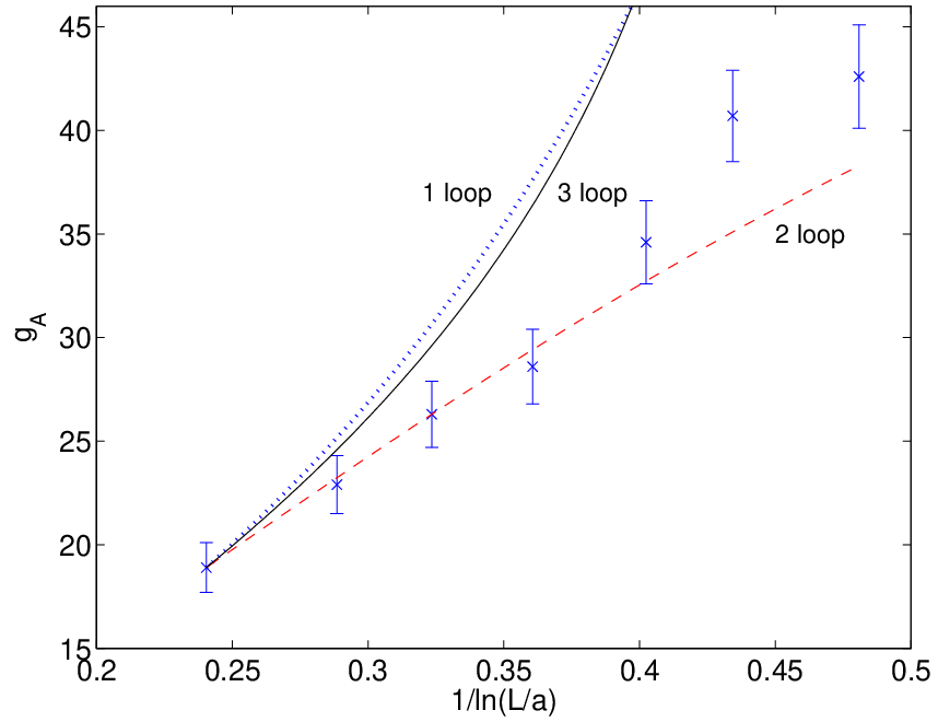
In Fig. 3 we study two couplings which we can compute with lower but still reasonably significant precision. On the left we see agreement between at with two loop perturbation theory, where no three loop term is available. Finally the right plot shows the fully antiperiodic at . Since relatively large momenta contribute here, the cutoff effects could be larger in this plot than in the previous ones. While we expect them to be still small for we cannot really disentangle them. We refer to the discussion in [7] that the perturbative artefacts, that could be specified at 1 and 2 loop order, are not relevant here.
5 Conclusions
In [5] a Monte Carlo algorithm was presented for simulating Aizenman’s reformulation of the Ising model as a statistical system of random currents on links [6]. This form has two advantages: (practical) absence of critical slowing down and the availability of a non-negative estimator for the connected four point function, that enters into the standard definition of renormalized interaction strength, without having to perform numerical cancellations. In the present paper we have generalized this from periodic boundary conditions in all four directions to arbitrary combinations of periodic and antiperiodic directions. Then the above mentioned estimator starts to fluctuate in sign but still yields good precision for one antiperiodic direction and system sizes as small as . With four antiperiodic directions the noise was found to much more degrade the possible precision. One and the same simulation produces results for all the boundary conditions considered here. For large the simulated graphs do not wind around the torus and the independence of results on the choice of boundary conditions becomes manifest.
In our previous work for the periodic case we have found, that the decay of the coupling strength with the UV cutoff (triviality) is not very well described by perturbation theory given the precision of our new method. This is a problem, because even very efficient numerical simulations cannot trace this decay over significant scale-ranges, if it happens only at the expected logarithmic rate. What it can only do is to confirm the matching with perturbation theory which can then be trusted all the way to the continuum. In [7] we have accumulated some evidence that the constant zero momentum mode that exists for periodic boundary conditions is the main source of nonperturbative behavior in small volumes. With at least one antiperiodic direction the smallest momentum is and all modes receive Gaussian damping independently of the mass term. In Fig. 1 we demonstrate that perturbation theory indeed works much better now.
In the present simulations we could determine with good precision the change in free energy caused by differing boundary conditions. Also these quantities can be related to renormalized couplings and probed numerically. As a nonvanishing tree level term has to be subtracted however, the precision is limited here. In perturbation theory only the first two universal terms are known for these couplings. Given these limitations also here reasonable agreement is found (Fig. 3, left plot).
Acknowledgements: We thank Peter Weisz for a careful reading of the manuscript. This work has emerged from the internship project of M. H. at Humboldt University and we thank the Ecole Normale Superieure (Paris) for financial support. U.W. acknowledges support by the DFG via SFB transregio 9.
Appendix A Proof of eq. (11)
We freeze to fixed values and then show for an arbitrary charge distribution the counting identity
| (34) |
where the large brackets are binomial coefficients. The sums here run over values from to independently for each . If and are not in the same percolation cluster made from bonds with , then vanishes and the same is true for for all , and thus both sides are zero. We thus only have to consider the case . Following Aizenman [6] (Lemma 3.2) we momentarily think of a graph of distinguishable lines drawn ‘over’ each link with (link-wise) cardinality . Then on both sides we count the number of distinct subsets which are such that the cardinalities and obey certain divergence constraints. The identity is proven now by constructing a one-to-one mapping between the respective subsets contributing on the right hand side and the left hand side.
Because of there is some chain of specific lines connecting and . If we now have some that contributes to the left hand side, then we map
| (35) |
One may now show that
- •
if satisfies the constraints of the left hand side of (34) then fulfills those on the right hand side,
- •
under the same mapping maps back to .
Therefore (34) is now established.
We now multiply both sides of (34) with where is arbitrary and is defined in (6). Then we sum over and change variables to and to derive
| (36) |
This may be used repeatedly to derive
| (37) |
with the short hand notation . To satisfy and , the four points must either belong to one or to two percolation clusters of . In the latter case it is easy to verify that vanishes while in the first case it equals . This may now be changed back to
| (38) |
Appendix B Perturbative expansion
B.1 Couplings based on correlations
We here report details on the computation of the expansion (in ) coefficients66 6 We count on our readers to not confuse these with momenta. and for the schemes using with defined in section 3.2. In terms of 1PI vertex functions our renormalized parameters read
| (39) |
| (40) |
| (41) |
with being the ‘wave function’ renormalization factor and all quantities are at finite . Standard bare perturbation theory gives (dropping subscripts here)
| (42) |
| (43) |
The capital letters stand for the usual Feynman diagrams for the two and four point functions up to two loops and are given explicitly below. The mass parameter in all propagators is the bare mass at this stage. The actual evaluation proceeds via the following sequence of steps,
| (44) |
| (45) |
| (46) |
Note that in
| (47) |
only integer momenta (e.g. ) are appropriate for even where is periodic for all . We form (dropping subscripts again)
| (48) |
and similarly
| (49) |
| (50) |
| (51) |
| (52) |
The Fourier transformations are performed as FFT on one coordinate direction after another and the whole 2 loop computation again has computational complexity only, see [7] for more details.
With these expressions we can write (omitting the remainders)
| (53) |
| (54) |
and
| (55) | |||||
In order to obtain as a function of and we have to combine now the last two equations to eliminate on the right hand sides. To the order considered and using
| (56) |
we arrive at
| (57) |
with
| (58) | |||||
| (59) |
and then at
| (60) |
with
| (61) | |||||
| (62) | |||||
In these formulae on the right hand sides is given by , of course, and in the arguments of refer to the mass value used here in the propagators that enter.
B.2 Couplings based on partition function ratios
We here work out the coefficients appearing in (31). The leading order is trivially given by
| (63) |
The first correction receives contributions from both the interaction term and from eliminating for the renormalized mass by (54) and we find after simple steps
| (64) |
with the mass here in both propagators. Numerical values are given in Table 6,
| 8 | 0.26076127 | 0.35227920 | 0.30274830 | 2.4978979 |
|---|---|---|---|---|
| 10 | 0.24731850 | 0.33411586 | 0.29837653 | 2.4880152 |
| 12 | 0.24059900 | 0.32490117 | 0.29621943 | 2.4832198 |
| 16 | 0.23423877 | 0.31612031 | 0.29419783 | 2.4787956 |
| 22 | 0.23052145 | 0.31096912 | 0.29302625 | 2.4762694 |
| 32 | 0.22836421 | 0.30797464 | 0.29234996 | 2.4748253 |
| 64 | 0.22693150 | 0.30598406 | 0.29190233 | 2.4738756 |
and asymptotic large Symanzik expansions for these cases are
| (65) |
| (66) |
| (67) |
| (68) |
References
- [1] M. Lüscher and P. Weisz, Scaling Laws and Triviality Bounds in the Lattice phi**4 Theory. 1. One Component Model in the Symmetric Phase, Nucl. Phys. B290 (1987) 25.
- [2] I. Montvay, G. Münster, and U. Wolff, Percolation Cluster Algorithm and Scaling Behavior in the four-dimensional Ising Model, Nucl. Phys. B305 (1988) 143.
- [3] N. Prokof’ev and B. Svistunov, Worm Algorithms for Classical Statistical Models, Phys. Rev. Lett. 87 (2001) 160601.
- [4] U. Wolff, Simulating the All-Order Strong Coupling Expansion I: Ising Model Demo, Nucl. Phys. B810 (2009) 491.
- [5] U. Wolff, Precision check on triviality of theory by a new simulation method, Phys. Rev. D79 (2009) 105002.
- [6] M. Aizenman, Geometric Analysis of phi**4 Fields and Ising Models (Parts 1 and 2), Commun. Math. Phys. 86 (1982) 1.
- [7] P. Weisz and U. Wolff, Triviality of theory: small volume expansion and new data, Nucl. Phys. B846 (2011) 316.
- [8] ALPHA Collaboration, U. Wolff, Monte Carlo Errors with less Errors, Comput. Phys. Commun. 156 (2004) 143.