Subdominant terms in the production of pairs
in proton-proton collisions
Abstract
At high-energies the gluon-gluon fusion is the dominant mechanism of production. This process was calculated in the NLO collinear as well as in the kt-factorization approaches in the past. We show that the present knowledge of gluon distributions does not allow to make a precise predictions for production at LHC, in particular at forward rapidities. In this paper we study production of pairs including several subleading mechanisms. This includes: , , , . In this context we use MRST-QED parton distributions which include photon as a parton in the proton as well as elastic photon distributions calculated in the equivalent photon approximation. We present distributions in the quark ( antiquark) rapidity and transverse momenta and compare them to the dominant gluon-gluon fusion contribution. We discuss also inclusive single and central diffractive processes using diffractive parton distribution found from the analysis of HERA diffractive data. As in the previous case we present distribution in () rapidity and transverse momentum. Finally we present results for exclusive central diffractive mechanism discussed recently in the literature. We show corresponding differential distributions and compare them with corresponding distributions for single and central diffractive components.
pacs
12.38.-t,14.65.DwI Introduction
In the past we have calculated inclusive cross section for heavy quarks production at hadron colliders. These calculations were performed using an approach based on the unintegrated parton distributions functions [1, 2]. It is known that gluon-gluon fusion is the dominant mechanism at high energy. However, other mechansims were not carefully studied in the literature.
It is the aim of this work to present contributions of several subleading terms usually neglected in the analysis of production. We wish to include contributions of photon-gluon (gluon-photon) as well as purely electromagnetic contributions of photon-photon fusion.
We wish to discuss also diffractive processes (single and central) in the framework of Ingelman-Schlein model corrected for absorption. Such a model was used in estimation of several diffractive processes [3, 4, 5, 6, 7, 8].
The absorption corrections turned out to be necessary to understand a huge Regge-factorization breaking observed in single and central production at Tevatron.
Recently a surprisingly large cross section for exclusive production has been reported [9]. Her we will show results for RHIC and LHC energies.
II Production of heavy quarks
In the leading-order (LO) approximation within the collinear approach the quadruply differential cross section in the rapidity of (), in the rapidity of () and the transverse momentum of one of them () can be written as
| (1) |
Above, and are the familiar (integrated) parton distributions in hadron and , respectively. There are two types of the LO subprocesses which enter Eq.(1): and . The first mechanism dominates at large energies and the second one near the threshold. In particular for the gluon-gluon fusion the cross section formula takes a simple form:
| (2) |
There are three (, and ) diagrams in the leading order [10].


The parton distributions are evaluated at: , , where . The formulae for matrix element squared averaged over the initial and summed over the final spin polarizations can be found e.g. in Ref.[10].
The inclusive heavy quark/antiquark production can be also calculated in the framework of the -factorization. In this approach transverse momenta of initial partons are included and emission of gluons is encoded in so-called unintegrated gluon distributions (UGDFs) [1].
In the leading-order (LO) approximation within the -factorization approach the quadruply differential cross section in the rapidity of (), in the rapidity of () and the transverse momentum of () and () can be written as
| (3) | |||
where and are so-called unintegrated gluon (parton) distributions. Now the unintegrated parton distributions must be evaluated at: , , where .
III Photon induced production of heavy quarks
III.1 MRST-QED parton distributions
As discussed above the dominant contributions are initiated by gluons or quarks and antiquarks. In general even photon can be a constituent of the proton. This was considered only in one work by Martin, Roberts, Stirling and Thorne [11]. Below we repeat the main aspects of their formalism.
The factorization of the QED-induced collinear divergences leads to QED-corrected evolution equations for the parton distributions of the proton [11]:
| (4) |
where
and the parton distributions fullfil momentum conservation:
| (5) |
III.2 Mechanisms with one or two photons
If the photon is a constituent of the nucleon then other mechanisms presented in Fig.2 are possible.


Here the cross section can be calculated similarly as for the gluon-gluon fusion. A corresponding triple differential cross section can be written as:
| (6) |
for gluon-photon, photon-gluon and photon-photon contributions, respectively. Compared to gluon-gluon case here only and diagrams occur.
The above contributions include only cases when nucleons do not survive a collision and nucleon debris is produced instead. The case when nucleon survives a collision has to be considered separately. In this case one can include corresponding photon distributions where extra ”el” index will be added to denote that situation. Corresponding contributions can be then written as:
| (7) |
The elastic contributions are calculated using Drees-Zepenfeld (elastic) parametrizations of photon fluxes [12] which include nucleon electromagnetic form factors.
IV Results
IV.1 Gluon distributions and small-x region and its relation to production
In Fig.3 we show three different leading-order gluon distributions from the literature [13, 11, 14] (left panel) and photon distributions [11] (right panel) as a function of longitudinal momentum fraction for a fixed scale 10 GeV relevant for production. Above 10-2 all the distributions coincide. For smaller values of they diverge and can be different by almost an order of magnitude. What are consequences of this divergence for pair production? This will be discussed below.


Before we go to cross sections in transverse momentum and rapidities, in Fig.4 we present distribution of the cross section in = log and = log for two different energies = 500 GeV (updated RHIC) and = 14 TeV (nominal LHC energy). One can clearly see that the and values are strongly correlated. Typical values at = 500 GeV are 0.5 10-2 and at = 14 TeV are 10-4. In the latter case ’s as small as 10-6 may appear in the forward or region. This is clearly a region of which was never studied so far.


Now let us present distributions in transverse momentum of (or ) for gluon-gluon fusion mechanism for different gluon distributions and different popular choices of scales (, invariant mass of the system ). We show our results for = 500 GeV (Fig.5) and = 14 TeV (Fig.6). One can clearly see that for some choices of gluon distribution function and scales the results for = 14 TeV are not physical. This shows how badly known are gluon distributions at the low .


IV.2 and subprocesses
In Fig.7 and in Fig.8, we show results for different gluon distribution functions for the RHIC energy = 500 GeV and nominal LHC energy = 14 TeV, respectively. At the LHC energy the results for different GDFs differ considerably which is a consequence of the small- region as discussed in the previous section. The differences at the nominal LHC energy = 14 TeV are particularly large which can be explained by the fact that a product of gluon distributions (both at small ) enters the cross section formula. A new measurement of at the nominal LHC energy will be therefore a severe test of gluon distributions at small and not too high factorization scales not tested so far. Similar uncertainties for the and are smaller as here only one gluon distribution appears in the corresponding cross section formula.


It is very difficult to quantify uncertainties related to the photon PDFs as only one set of PDFs includes photon as a parton of the proton. Here the isospin symmetry violation (not well known at present) would be an useful limitation. Our collection of the results for the photon induced mechanisms show that they are rather small and their identification would be rather difficult as the different distributions are very similar to those for the gluon-gluon fusion. Our intension here is to document all the subleading terms in one publication. Our etimation shows that the sum of all the photon induced terms is less than 0.5 % and is by almost 2 orders of magnitude smaller than the uncertainties of the dominant leading-order gluon-gluon term.
V Single and central diffraction
V.1 Formalism
The mechanisms of the ordinary as well as diffractive production of heavy quarks () are shown in Figs.9,10.


In the following we apply the Ingelman and Schlein approach11 1 In the literature also dipole model was used to estimate diffractive production [15]. . In this approach one assumes that the Pomeron has a well defined partonic structure, and that the hard process takes place in a Pomeron–proton or proton–Pomeron (single diffraction) or Pomeron–Pomeron (central diffraction) processes. We calculate triple differential distributions as
| (9) |
| (10) |
| (11) |
for ordinary, single-diffractive and central-diffractive production, respectively.
We do not calculate the higher-order contributions and include them effectively with the help of a so-called -factor. We have checked that this procedure is precise enough in the case of ordinary Drell-Yan process. The -factor is calculated as for the Drell-Yan process
Here the running coupling constant is evaluated at .
The ’diffractive’ quark distribution of flavour can be obtained by a convolution of the flux of Pomerons and the parton distribution in the Pomeron :
The flux of Pomerons enters in the form integrated over four–momentum transfer
| (13) |
with being kinematic boundaries.
Both pomeron flux factors as well as quark/antiquark distributions in the pomeron were taken from the H1 collaboration analysis of diffractive structure function and diffractive dijets at HERA [16]. The factorization scale for diffractive parton distributions is taken as .
V.2 Results
Let us start presentation of our results for diffractive mechanisms.
In Fig.11 we show transverse momentum distributions of charm quarks (or antiquarks). The distribution for single diffractive component is smaller than that for the inclusive gluon-gluon fusion by almost two orders of magnitude. Our results include gap survival factor. Corresponding values are taken the same as in Ref. [17]. The cross section for inclusive central diffractive component is smaller by additional order of magnitude. In addition we show the cross section for fully22 2 Although the calculation assumes simple state hadronization leads to more complicated states [9]. exclusive mechanism discussed in section VI. Below we shall use the following notation: for standard nondiffractive component, or for single diffractive and for central diffractive components.


In Fig.13 we show similar results for nominal LHC energy = 14 TeV. The situation and the interrelations between different components is qualitatively the same. Here somewhat smaller gap survival factors were used [17]. The distributions for all components are somewhat broader than those for the RHIC energy shown above.


In Fig.14 we show distributions in quark (antiquark) rapidity. We show separately contributions of two different single-diffractive components, which give the same distributions in transverse momentum in Fig.13. When added together they produce a distribution similar in shape to the standard inclusive case. Here different parton distributions functions give similar result. The distributions for different proton gluon distributions are quite different. This was already observed when discussing photon induced components in section VI.


Also two dimensional distributions can be interesting as here different mechanisms may occupy different parts of the phase space.
In Fig.15 we show distributions in the rapidity of the pair and quark-antiquark invariant mass. Although the distributions are somewhat different the differences occur in the regions which may be difficult to measure. The spread in the pair rapidity for the central diffractive component is much smaller then that for the inclusive case.


Finally we show distributions in quark and antiquark rapidities. The distribution for the inclusive central diffractive mechanism are concentrated at midrapidities. This is a rather universal feature of diffractive processes.


The cross section for single and central diffraction is rather small. However, a very specific final state should allow for its identification by imposing special conditions on the one-side (single-diffractive process) or on both-side (central diffractive process) rapidity gaps. We hope that such an analysis is possible at LHC. Special care should be devoted to the observation of the exclusive production where the observation of mesons associated by a few pions would be a proper signal [18]. Without a special analysis of the final state multiplicity the exclusive production may look like an inclusive central diffraction. At present there is no analysis of the final state production for the exclusive .
A comparison of cross sections for both components will be done in the next section.
VI Exclusive central diffractive production of
There is recently a growing theoretical interest in studying central exclusive mechanisms of different particles production at high energies, which constitute a special category of double-diffractive processes. To date, only a few exclusive processes have been measured so far at the Tevatron collider (see [19] and references therein). In particular, central exclusive production (CEP) of the Higgs boson is a flag process of special interest and importance in the upcoming Higgs searches at the LHC (see e.g. Ref. [20, 21]).
Generally, in the case of the central exclusive production with the leading protons, the central system should necessarily be produced in the color singlet state, such that the proton remnants and the system are disconnected in the color space and their hadronisation occurs independently giving rise to rapidity gaps [22]. From the experimental point of view, CEP procesess are very attractive, because of the rare clean experimental environment, related to selection rule, and great mass resolution of the centraly produced object. Such unique features give a new possibility to exploit high branching ratio decay channel of the Higgs boson, which is rather impossible in standard inclusive measurements, due to very large QCD background. Therefore, the QCD mechanism of central exclusive heavy quark dijets is a source of the irreducible background to the exclusive Higgs boson production.
Central exclusive production of and pairs was studied in detail in our previous papers [9, 20, 21]. In these calculations the reaction, illustrated in Fig. 17, was considered as a genuine 4-body process with exact kinematics. The applied perturbative model of theoretical predictions is based on the Khoze-Martin-Ryskin (KMR) approach used previously for the exclusive Higgs boson production [23]. Total cross sections and differential distributions for heavy quarks are calculated by using -factorization approach with help of the KMR unintegrated gluon distribution functions.
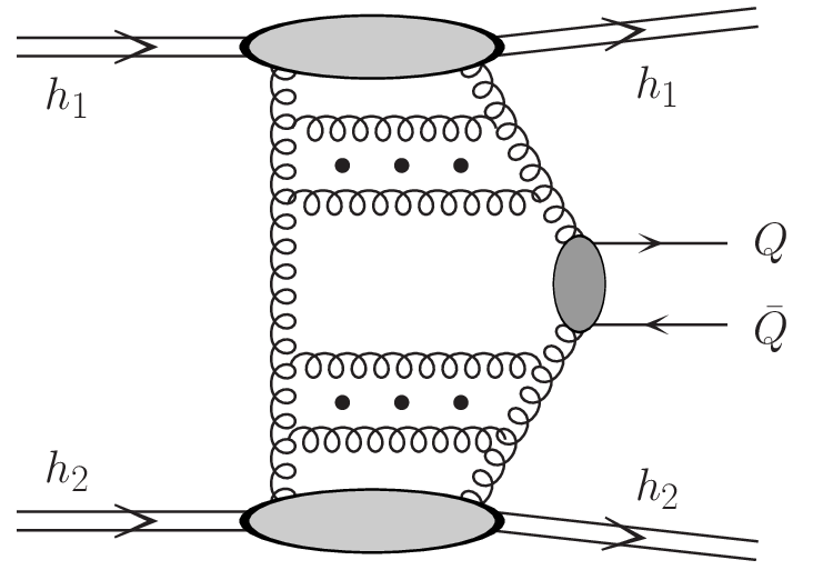

This QCD model works very good in the case of exclusive dijets and charmonia production, what was confirmed by CDF data [24, 25, 26, 27]. However, estimated uncertainties related to gluon densities, factorization and renormalization scales, as well as due to absorption corrections are quite large. It makes the situation somewhat clouded and prevents definite conlcusions, especially in the case of the exclusive production of heavy quark pairs. In this context, the promising idea, how to clarify and calibrate purely-known parameters of the theoretical model, is to study cross section by exclusive measurements of meson pairs. Such experimental studies are being performed now at Tevatron and could be also available in Run II experiments at RHIC and at LHC.
Therefore, it is also very interesting, from both, theoretical and experimental side, to compare mechanism of central exclusive production of charm quarks with standard single and double diffractive processes. Such an analysis of differential cross sections has never been done before but could bring important informations about differences in kinematics and in production rates between them, what is crucial for future measurements.
According to the KMR approach [23, 28, 29] we write the amplitude of the exclusive diffractive pair production as
where are helicities of heavy and , respectively, are the momentum transfers along each proton line, and are the transverse momenta and the longitudinal momentum fractions for active and screening gluons, respectively. Above are the off-diagonal UGDFs related to both nucleons. The vertex factor is the production amplitude of a pair of massive quark and antiquark with helicities , and momenta , , respectively. The longitudinal momentum fractions of active gluons are calculated based on kinematical variables of outgoing quark and antiquark: and , where and are transverse masses of the quark and antiquark, respectively, and and are corresponding rapidities.
The off-diagonal UGDFs are written as [30]
| (14) |
where accounts for the single skewed effect [31]. The factor here cannot be calculated from first principles in the most general case of off-diagonal UGDFs. It can be estimated only in the case of off-diagonal collinear PDFs when and and then . In the considered kinematics the diagonal unintegrated densities can be written in terms of the conventional (integrated) densities as [30]
| (15) |
where is the conventional Sudakov survival factor which suppresses real emissions from the active gluon during the evolution, so the rapidity gaps survive.
In the framework of the -factorization approach [32] the hard subprocess gauge invariant amplitude reads
| (16) | |||
where is the c.m.s. proton energy, are the color group generators in the fundamental representation, and are on-shell quark and antiquark spinors, respectively, and are the effective vertices arising from the Feynman rules in quasi-multi-Regge kinematics (QMRK) approach [33]:
| (17) | |||
where is the effective three-gluon vertex. The effective -vertices are canceled out when projecting the production amplitude Eq. (16) onto the color singlet state. Since we will adopt the definition of gluon polarization vectors proportional to transverse momenta , i.e. (see below), then we must take into account the longitudinal momenta in the numerators of effective vertices (see Eq. (17)).
The SU(3) Clebsch-Gordan coefficient in Eq. (16) projects out the color quantum numbers of the pair onto the color singlet state. Factor provides the averaging of the matrix element squared over intermediate color states of quarks.
Therefore, we have the following amplitude
| (18) |
In the present calculations we use the GJR08 set of collinear gluon distributions [34]. In the analogy to the CEP of Higgs boson, where renormalization and factorization scales are advocated to be [35], we apply the following prescription . Absorption corrections to the bare amplitude, which are necessary to be taken into account (to ensure exclusivity of the process), are included approximately by multiplying the cross section by the gap survival factors for RHIC and for the LHC energy. More details about exclusive production of heavy quarks can be found in our original paper [9]. Let us come now to presentation of our results.
In Fig.18 we show rapidity distribution of quarks from the exclusive mechanism shown in Fig. 17 (solid line). We show the results for leading order (upper curves) and next-to-leading order collinear gluon distributions [34]. We observe large difference of results for LO and NLO gluon distribution especially at LHC. For comparison we show the contribution of central diffractive component discussed in section V. In this calculation we have included gap survival factors = 0.1 for = 500 GeV and = 0.03 for = 14 TeV. The cross section for the exclusive mechanism is similar to that for the inclusive central diffractive mechanism. The exclusive production starts to dominate only at large quark rapidities. Therefore a measurement of the cross section with double (both side) rapidity gaps may be not sufficient to single out the exclusive mechanism. Clearly other cuts would be necessary.


Corresponding distributions in the quark ( antiquark) transverse momentum are shown in Fig.19. The distribution for exclusive component extends to higher transverse momentum than that for the central inclusive diffractive one. A lower cut on quark (D meson) transverse momentum may therefore help to identify the exclusive component but will exclude a measurment of the integrated cross section for this component. A detailed Monte Carlo studies of final states of both components may help to find a better criterion to separate experimentally the two components.


VII Conclusions
In the present paper we have calculated differential distributions for different subdominant contributions usually neglected in the literature when calculating production of pairs.
Single and double photon induced processes are first class of mechanisms considered here. In calculating single particle distributions we have used a special set of parton distributions which includes photon as a parton of the proton. The calculation of the cross section is therefore very similar to that for the gluon-gluon fusion. The difference is only in color factors and a lack of the s-channel diagrams for photon induced processes. We have also included contributions when emitted photon which enters a hard process leaves a proton in a ground state. Those “elastic” mechanisms give similar contribution as the “deeply inelastic” mechanisms considered in the QCD-improved parton model. We have found that although individual contributions are very small, when added together they can give cross section of about 1 % of the inclusive one dominated by gluon-gluon fusion. In our analysis we have neglected resonance contributions when the photon leaves the remaining object in a proton excited state, e.g. in (1220) resonance or other nucleon resonances.
We have also discussed single and central diffractive production of pairs in the Ingelman-Schlein model. In these calculations we have included diffractive parton distributions obtained by the H1 collaboration at HERA and absorption effects neglected in some early calculations in the literature. The absorption effects which are responsible for the naive Regge factorization breaking cause that the cross section for diffractive processes is much smaller than that for the fully inclusive case, but could be measured at RHIC and LHC by imposing special condition on rapidity gaps.
Finally we have discussed a fully exclusive diffractive production of . It was advocated recently that the cross section for this mechanism may be substantial. We have found here that both at RHIC and LHC its contribution is smaller than that for single diffractive one. In our opinion it is very timely to analyze if this contribution could be measured. This equires an analysis of the final state. We expect that the final state in single and exclusive production are different enough to set criteria to pin down the fully exclusive component. It is, however, not obvious if the central diffractive and purely exclusive mechanisms could be differentiated experimentally. They may look similar as far as rapidity gap structure is considered. We predict that the total contribution of central diffractive mechanism is similar to that for the exclusive one. In contrast the final state multiplicity can be expected to be different. A better analysis requires a Monte Carlo studies.
We have not discussed an impact of diffractive mechanisms considered in the present paper on the fully inclusive cross section for pair production. This is a rather difficult task and goes beyond the scope of the present paper.
Acknowledgments
We are indebted to Wolfgang Schäfer and Roman Pasechnik for interesting conversions. This work was partially supported by the polish grant N N202 237040.
References
- [1] M. Łuszczak and A. Szczurek, Phys. Rev. D73 (2006) 054028.
- [2] M. Łuszczak, R. Maciuła, A. Szczurek, Phys. Rev. D79 (2009) 034009
- [3]
P. Bruni, G. Ingelman, Phys.Lett.B311 317 (1993);
L. Alvero, J.C. Collins, J. Terron and J.J. Whitmore, Phys. Rev. D59 (1999) 074022;
R.J.M. Covolan and M.S. Soares, Phys. Rev. D60 (1999) 054005, Phys. Rev. D67 (2003) 017503;
M.B. Gay Ducati, M.M. Machado and M.V.T Machado, Phys. Rev. D75 (2007) 114013. - [4] G. Ingelman, P.E. Schlein, Phys.Lett.B152 256 (1985).
- [5]
M. Heyssler, Z. Phys. C73 (1997) 299;
M.B. Gay Ducati, M.M. Machado and M.V.T Machado, Phys. Rev. D81 (2010) 054034. - [6]
R. Enberg, G. Ingelman, N. Timneanu, Phys.Rev.D67 (2003) 011301;
S. Erhan, V.T. Kim and P.E. Schlein,[arXiv:hep-ph/0312342];
M.B. Gay Ducati, M.M. Machado and G.G. Silveira,[arXiv:hep-ph/1101.5602]. - [7]
A. Berera, J.C. Collins, Nucl. Phys. B474 183 (1996);
R.J.M. Covolan and M.S. Soares, Phys. Rev. D67 (2003) 077504. - [8] M.V.T. Machado, Phys. Rev. D76 (2007) 054006.
- [9] R. Maciuła, R. Pasechnik and A. Szczurek, Phys. Lett. B685 (2010) 165.
- [10] V. Barger and R. Phillips, ”Collider Physics”, Addison-Wesley Publishing Company, Redwood Cite, 1987
- [11] A.D. Martin, R.G. Roberts, W.J. Stirling, R.S. Thorne, Eur.Phys.J.C39:155-161,2005
- [12] M. Drees and D. Zeppenfeld, Phys. Rev. D39 (1998) 2536
- [13] M. Gluck, E. Reya, A. Vogt, Eur.Phys.J. C5 (1998) 461-470.
- [14] A.D. Martin, W.J. Stirling, R.S. Thorne, G. Watt, Eur.Phys.J.C39 C63:189-285,2009
- [15] B. Kopeliovich, Phys. Lett. B447 (1999) 308.
- [16] A. Aktas et al. [H1 Collaboration], Eur. Phys. J. C 48, 715 (2006) [arXiv:hep-exp/0606004].
- [17] G. Kubasiak and A. Szczurek, Phys. Rev. D84 (2011) 014005.
- [18] a paper in preparation.
- [19] M.G. Albrow, T.D. Coughlin and J.R. Forshaw, arXiv:hep-ph/1006.1289.
- [20] R. Maciuła, R. Pasechnik and A. Szczurek, Phys. Rev. D83, 054014 (2011)
- [21] R. Maciuła, R. Pasechnik and A. Szczurek, Phys. Rev. D83, 114034 (2011)
- [22] R. Enberg, G. Ingelman, A. Kissavos et al., Phys. Rev. Lett. 89, 081801 (2002).
- [23]
V. A. Khoze, A. D. Martin and M. G. Ryskin,
Phys. Lett. B401, 330 (1997);
A. B. Kaidalov, V. A. Khoze, A. D. Martin and M. G. Ryskin, Eur. Phys. J. C33, 261 (2004). - [24] A. Dechambre, O. Kepka, C. Royon and R. Staszewski, Phys. Rev. D83, 054013 (2011)
- [25] R. Maciuła, R. Pasechnik and A. Szczurek, arXiv:1109.5517.
- [26] R. S. Pasechnik, A. Szczurek and O. V. Teryaev, Phys. Rev. D78, 014007 (2008)
- [27]
R. S. Pasechnik, A. Szczurek and O. V. Teryaev,
Phys. Lett. B680, 62 (2009);
R. S. Pasechnik, A. Szczurek and O. V. Teryaev, Phys. Rev. D 81, 034024 (2010). - [28]
A. De. Roeck et al., Eur. Phys. J. C25 (2002) 391;
S. Heinemeyer et al., Eur. Phys. J. C53 (2008) 231. - [29] A. G. Shuvaev, V. A. Khoze, A. D. Martin and M. G. Ryskin, Eur. Phys. J. C56, 467 (2008) [arXiv:0806.1447 [hep-ph]].
- [30] A. D. Martin and M. G. Ryskin, Phys. Rev. D64, 094017 (2001).
- [31] A. G. Shuvaev, K. J. Golec-Biernat, A. D. Martin and M. G. Ryskin, Phys. Rev. D60, 014015 (1999).
- [32]
P. Hagler, R. Kirschner, A. Schafer, L. Szymanowski and O. Teryaev,
Phys. Rev. D62, 071502 (2000);
P. Hagler, R. Kirschner, A. Schafer, L. Szymanowski and O. V. Teryaev, Phys. Rev. Lett. 86, 1446 (2001). - [33] V. S. Fadin and L. N. Lipatov, Nucl. Phys. B477, 767 (1996)
- [34] M. Glück, D. Jimenez-Delgado, E. Reya, Eur. Phys. J. C53, 355 (2008).
- [35] T.D. Coughlin and J.R. Forshaw, JHEP 1001 (2010) 121.