跳到论文正文
W Papers独立论文阅读器 arXiv:1109.5779 论文正文 计算阅读时间 · 0%
引用这篇论文根据当前论文元数据生成,正式投稿前建议核对。


License: arXiv.org perpetual non-exclusive license
arXiv:1109.5779v2 [cs.IT] 31 Oct 2011

The Degrees of Freedom Region of the MIMO Interference Channel with Shannon Feedback

Chinmay S. Vaze and Mahesh K. Varanasi ††thanks: This work was supported in part by NSF EAGER Grant CCF-1144026. The authors are with the Department of Electrical, Computer, and Energy Engineering, University of Colorado, Boulder, CO 80309-0425 USA (e-mail: Chinmay.Vaze, varanasi@colorado.edu). The material in this paper was presented in part at the $49ˆth$ Annual Allerton Conference on Communication, Control, and Computing, Monticello, IL, USA, Sep. 28-30, 2011.
Abstract

The two-user multiple-input multiple-output (MIMO) fast-fading interference channel (IC) with an arbitrary number of antennas at each of the four terminals is studied under the settings of Shannon feedback, limited Shannon feedback, and output feedback, wherein all or certain channel matrices and outputs, or just the channel outputs, respectively, are available to the transmitters with a finite delay. While for most numbers of antennas at the four terminals, it is shown that the DoF regions with Shannon feedback and for the limited Shannon feedback settings considered here are identical, and equal to the DoF region with just delayed channel state information (CSIT), it is shown that this is not always the case. For a specific class of MIMO ICs characterized by a certain relationship between the numbers of antennas at the four nodes, the DoF regions with Shannon and the limited Shannon feedback settings, while again being identical, are strictly bigger than the DoF region with just delayed CSIT. To realize these DoF gains with Shannon or limited Shannon feedback, a new retrospective interference alignment scheme is developed wherein transmitter cooperation made possible by output feedback in addition to delayed CSIT is employed to effect a more efficient form of interference alignment than is feasible with previously known schemes that use just delayed CSIT. The DoF region for just output feedback, in which each transmitter has delayed knowledge of only the receivers’ outputs, is also obtained for all but a class of MIMO ICs that satisfy one of two inequalities involving the numbers of antennas.

Index Terms: 
Degrees of freedom, delayed CSIT, feedback, interference channel, interference alignment, MIMO, Shannon feedback.

I Introduction

The characterization of the capacity of channels with feedback, where the channel outputs are known to the transmitter(s) with a finite delay, is a classical problem in information theory. For example, it is well known that feedback can not increase the capacity of a memoryless point-to-point channel [1]. Moreover, feedback can not increase the capacity of a point-to-point channel with additive, correlated Gaussian noise by more than one bit [1]. Interestingly, multi-user channels exhibit a different behavior. In particular, feedback can enhance the capacity of even the memoryless multiple access channel (MAC) [2, 3] but again this improvement is bounded for the Gaussian MAC [3]. There has also been much interest in characterizing the capacity region of other memoryless networks with feedback such as the broadcast channel (BC) [4]. However, due to the apparent intractability of such problems for more complex topologies, capacity approximations have been sought. Of these approximate capacity metrics, the degrees of freedom (DoF) region has received considerable attention. The DoF region denotes the rate of growth of the capacity region with respect to the logarithm of the signal-to-noise ratio (SNR) in the limit of asymptotically high SNR. For example, it can be deduced from [5] that for the 22-user Gaussian MIMO IC output feedback can not enhance the DoF region when there is perfect and instantaneous CSIT. In [6], the feedback capacity region is characterized to within a constant gap of 22 bits for the single-antenna (or SISO) IC. Further, it is well known that feedback fails to improve the DoF regions of the Gaussian MIMO MAC and the Gaussian MIMO BC. It is not yet known if there are networks with instantaneous CSIT for which (output) feedback enhances the DoF region.

While the DoF of networks under the idealized assumptions of perfect, often global, and instantaneous CSIT have been well studied for numerous networks, the much more conservative setting of isotropic fading with transmitters having no CSIT has recently been extensively studied as well [7, 8, 9, 10, 11, 12, 13, 14]. Networks without CSIT but with (output) feedback have also been considered from which it is known that in the absence of CSIT feedback can enhance the DoF regions of the KK-user BC [15, 16, 17], the 22-user SISO X channel [18], and 33-user SISO IC [18, 10]. Thus, unlike the instantaneous CSIT case, feedback can be beneficial even from the DoF perspective when there is no CSIT. This suggests that the benefit of feedback depends critically on the availability of CSIT since it is vastly different at the two extremes of having instantaneous CSIT and having no CSIT whatsoever.

Moving beyond models that are either too idealized on the one extreme, or too conservative on the other, we consider here the delayed CSIT model wherein the channel state varies independently across time and the transmitters know perfectly the past channel states (cf. [15, 18, 16]). For such a setting we investigate the question of whether output feedback can improve the DoF region. Clearly, this question can be definitively answered only for networks for which the DoF with (just) delayed CSIT are known, of which there are but few. Of all networks for which the DoF are known except for the MIMO IC, this question has so far been answered in the negative. In particular, it is known that with delayed CSIT output feedback can not increase (a) the sum-DoF of the KK-user MISO BC with at least KK transmit antennas [15], (b) the DoF region of the 22-user MIMO BC [16], (c) the sum-DoF of the 33-user MIMO BC with NN antennas at all three receivers and at most 2​N2N antennas at the transmitter [17] and (d) the 2×2×22\times 2\times 2 interference network [19].

Refer to caption
Fig. 1: The (M1,M2,N1,N2)(M_{1},M_{2},N_{1},N_{2}) MIMO IC with Shannon Feedback

The only other exact characterization for the DoF region with (just) delayed CSIT is provided by the authors in [20] for the two-user MIMO IC with an arbitrary number of antennas at each of the four terminals. Consequently, by obtaining the complete DoF region of this general two-user MIMO IC with delayed CSIT and output feedback (i.e., under Shannon feedback), and showing that for some cases there is a strict enhancement of the DoF region over that with just delayed CSIT, we answer the question of whether output feedback can enhance the DoF region of a network with delayed CSIT for the first time in the affirmative.

In particular, it is shown here that if MiM_{i} and NiN_{i}, respectively, denote the number of antennas at the it​hi^{th} transmitter and the it​hi^{th} receiver of a two-user MIMO IC, then the DoF region with Shannon feedback is strictly bigger than the corresponding delayed-CSIT DoF region, if and only if one of the two inequalities, namely,

M1>N1+N2−M2>N1>N2>M2>N2​N2−M2N1−M2M_{1}>N_{1}+N_{2}-M_{2}>N_{1}>N_{2}>M_{2}>N_{2}\frac{N_{2}-M_{2}}{N_{1}-M_{2}}

or its symmetric counterpart (obtained by switching the user indices), holds. For MIMO ICs for which neither of these two inequalities holds output feedback does not improve the delayed CSIT DoF region.

To derive our main result, we first obtain an outer-bound to the DoF region with Shannon feedback. This outer bound is then shown to be achievable for all but the above described class of MIMO ICs using just delayed CSIT. For the class where the DoF region is strictly larger than that with delayed CSIT, we develop a new retrospective interference alignment scheme in which each transmitter – using the side information available to it – reconstructs and transmits the previously transmitted signal of the other transmitter to provide an opportunity to its paired receiver to cancel the interference it encountered at a previous time instant, while simultaneously delivering new useful linear combinations to the unpaired receiver. Consequently, Shannon feedback induces a new form of transmitter cooperation which is key to realizing the DoF gains attainable with Shannon feedback over that with just delayed CSIT.

Moreover, it is seen that to achieve this more efficient interference alignment all of the channel matrices and outputs are not needed at both transmitters. In particular, two limited Shannon feedback settings are described that are sufficient to achieve the DoF region with Shannon feedback. It is also observed that if in addition to delayed CSIT the feedback is allowed to be some designable function of past channel outputs and states, a setting that is more optimistic than Shannon feedback, the DoF region doesn’t expand over that of the DoF region in the Shannon feedback case. Furthermore, with just output feedback without any form of CSIT, it is shown that the DoF region is the same as that for delayed CSIT with the exception of a class of MIMO ICs characterized by one of two inequalities involving the numbers of antennas at the four terminals. For this class, the DoF region remains an open problem at this time.

The rest of the paper is organized as follows. Section II-A describes the model of MIMO IC under various assumptions about feedback, states the main results of this work on the DoF regions under these assumptions and provides an example of the new retrospective interference alignment scheme. Proofs of the results are contained in Sections III and IV and the appendix.

II Channel Models, Main Results, and IA with Shannon Feedback

In Section II-A, the MIMO IC model with Shannon feedback, limited Shannon feedback, output feedback and designable Shannon feedback are described. Section II-B contains the main results on the DoF regions under these settings. In Section II-C, we discuss how interference alignment can be achieved with Shannon and limited Shannon feedback. Section II-D provides some insight on the main results.

II-A The MIMO IC with Shannon Feedback

The MIMO IC consists of two transmitters, denoted as T1 and T2, and their corresponding receiver, labeled R1 and R2, respectively, as in Fig. 1. The (M1,M2,N1,N2)(M_{1},M_{2},N_{1},N_{2}) MIMO IC is defined via the input-output relationships

Y1​(t)\displaystyle Y_{1}(t) =\displaystyle= H11​(t)​X1​(t)+H12​(t)​X2​(t)+W1​(t),\displaystyle H_{11}(t)X_{1}(t)+H_{12}(t)X_{2}(t)+W_{1}(t), (1)
Y2​(t)\displaystyle Y_{2}(t) =\displaystyle= H21​(t)​X1​(t)+H22​(t)​X2​(t)+W2​(t),\displaystyle H_{21}(t)X_{1}(t)+H_{22}(t)X_{2}(t)+W_{2}(t), (2)

where, at time tt, Yi​(t)∈ℂNi×1Y_{i}(t)\in\mathbb{C}^{N_{i}\times 1} is the signal received by the it​hi^{th} receiver; Xi​(t)∈ℂMi×1X_{i}(t)\in\mathbb{C}^{M_{i}\times 1} is the signal transmitted by the it​hi^{th} transmitter; Hi​j​(t)∈ℂNi×MjH_{ij}(t)\in\mathbb{C}^{N_{i}\times M_{j}} is the channel matrix between the it​hi^{th} receiver and the jt​hj^{th} transmitter; Wi​(t)∈ℂNi×1W_{i}(t)\in\mathbb{C}^{N_{i}\times 1} is the additive white Gaussian noise at the it​hi^{th} receiver; and there is a power constraint of PP on the transmit signals, i.e., 𝔼​‖Xi​(t)‖2≤P\mathbb{E}||X_{i}(t)||^{2}\leq P ∀\forall i,ti,t.

Refer to caption
Fig. 2: Comparison of the DoF regions of a MIMO IC

For simplicity, we study here the case of additive white Gaussian noise, i.e., all entries of Wi​(t)W_{i}(t), i=1,2i=1,2, are independent and identically distributed (i.i.d.) according the complex normal distribution with zero-mean and unit-variance (denoted, henceforth, as 𝒞​𝒩​(0,1)\mathcal{C}\mathcal{N}(0,1)). Further, we assume that the channel matrices are i.i.d. Rayleigh faded, i.e., all elements of all channel matrices are i.i.d. according to 𝒞​𝒩​(0,1)\mathcal{C}\mathcal{N}(0,1) distribution (denoted as i.i.d. ∼𝒞​𝒩​(0,1)\sim\mathcal{C}\mathcal{N}(0,1)). Next, it is assumed that the realizations of additive noises and channel matrices are i.i.d. across time and that they are mutually independent of each other.

Throughout this paper, both receivers are taken to know all channel matrices perfectly. Since there is no delay constraint on decoding it is assumed, without loss of generality, that CSI is available instantaneously to the receivers. Further, all terminals are always assumed to know the distribution of the channel matrices.

We start by defining the term Shannon feedback (cf. [18]) and later consider other types of feedback. Here, the two transmitters are assumed to know the channel matrices and the channel outputs perfectly with a finite delay. This delay is taken to be of 11 symbol time without loss of generality. In particular, the channel matrices {Hi​j​(t)}i,j=12\{H_{ij}(t)\}_{i,j=1}^{2} and the channel outputs Y1​(t)Y_{1}(t) and Y2​(t)Y_{2}(t) are taken to be known perfectly to both transmitters at time t+1t+1.
Notation: For n≥0n\geq 0, H¯​(n)=△{H11​(t),H12​(t),H21​(t),H22​(t)}t=1n\overline{H}(n)\stackrel{{\scriptstyle\triangle}}{{=}}\big\{H_{11}(t),H_{12}(t),H_{21}(t),H_{22}(t)\big\}_{t=1}^{n} if n≥1n\geq 1 and H¯​(n)=ϕ\overline{H}(n)=\phi (ϕ=\phi= some constant) if n=0n=0. Similarly, for each i∈{1,2}i\in\{1,2\}, Y¯i​(n)={Yi​(t)}i=1n\overline{Y}_{i}(n)=\{Y_{i}(t)\}_{i=1}^{n} if n≥1n\geq 1 and Y¯i​(n)=ϕ\overline{Y}_{i}(n)=\phi if n=0n=0.

Let ℳ1\mathcal{M}_{1} and ℳ2\mathcal{M}_{2} be two independent messages to be sent by T1 and T2, respectively, over a block length of nn, where the message ℳi\mathcal{M}_{i} is intended for the it​hi^{th} receiver. It is assumed that ℳi\mathcal{M}_{i} is distributed uniformly over a set of cardinality 2n​Ri​(P)2^{nR_{i}(P)}, Ri​(P)≥0R_{i}(P)\geq 0, when there is a power constraint of PP at the transmitters. A coding scheme for blocklength nn consists of two encoding functions fi(n)={fi,t(n)}t=1nf_{i}^{(n)}=\{f_{i,t}^{(n)}\}_{t=1}^{n}, i=1,2i=1,2, such that

Xi​(t)=fi,t(n)​(ℳi,H¯​(t−1),Y¯1​(t−1),Y¯2​(t−1))​ with ​𝔼​‖Xi​(t)‖2≤P​∀i,t,X_{i}(t)=f_{i,t}^{(n)}\Big(\mathcal{M}_{i},\overline{H}(t-1),\overline{Y}_{1}(t-1),\overline{Y}_{2}(t-1)\Big)\mbox{ with }\mathbb{E}||X_{i}(t)||^{2}\leq P~\forall~i,t,

and two decoding functions such that

ℳ^i=gi(n)​(Y¯i​(n),H¯​(n))​ where ​i∈{1,2}.\hat{\mathcal{M}}_{i}=g_{i}^{(n)}\Big(\overline{Y}_{i}(n),\overline{H}(n)\Big)\mbox{ where }i\in\{1,2\}.

A rate tuple (R1​(P),R2​(P))\big(R_{1}(P),R_{2}(P)\big) is said to be achievable if there exists a sequence (over nn) of coding schemes such that probability of ℳ1≠ℳ^1\mathcal{M}_{1}\not=\hat{\mathcal{M}}_{1} or ℳ2≠ℳ^2\mathcal{M}_{2}\not=\hat{\mathcal{M}}_{2} tends to zero as n→∞n\to\infty.

The capacity region 𝒞⁡(P)\mathcal{C}(P) is defined to be the set of all achievable rate tuples (R1​(P),R2​(P))\big(R_{1}(P),R_{2}(P)\big) when the power constraint at the transmitters is PP. The DoF region with Shannon feedback is defined as

𝐃S=△{(d1,d2)∈ℝ+2|∀(w1,w2)∈ℝ+2,\displaystyle\mathbf{D}^{\rm S}\stackrel{{\scriptstyle\triangle}}{{=}}\Biggl\{(d_{1},d_{2})\in\mathbb{R}^{2}_{+}\Bigl|~\forall~(w_{1},w_{2})\in\mathbb{R}^{2}_{+},\Biggr.
w1d1+w2d2≤lim supP→∞1log2⁡P[sup(R1​(P),R2​(P))∈𝒞⁡(P){w1R1(P)+w2R2(P)}]},\displaystyle{}\Biggl.~~w_{1}d_{1}+w_{2}d_{2}\leq\limsup_{P\to\infty}\frac{1}{\log_{2}P}\Biggl[\sup_{\big(R_{1}(P),R_{2}(P)\big)\in\mathcal{C}(P)}\Big\{w_{1}R_{1}(P)+w_{2}R_{2}(P)\Big\}\Biggr]\Biggr\},

where ℝ+2\mathbb{R}^{2}_{+} denotes the set of pairs of non-negatives real numbers, and lim supP→∞\limsup_{P\to\infty} stands for the limit superior [21] as P→∞P\to\infty. It can be easily proved that the DoF region 𝐃S\mathbf{D}^{\rm S} is closed [21] and convex [1].

Consider next the MIMO IC under four other settings defined below.

  • •

    Designable Shannon feedback: both transmitters know the channel matrices {Hi​j​(t)}i,j\{H_{ij}(t)\}_{i,j} and modified channel outputs Y~1​(t)\tilde{Y}_{1}(t) and Y~2​(t)\tilde{Y}_{2}(t) at time t+1t+1 (in general, with some finite delay), where, for each i∈{1,2}i\in\{1,2\}, Y~i​(t)∈ℂNi×1\tilde{Y}_{i}(t)\in\mathbb{C}^{N_{i}\times 1} is a deterministic function of Y¯i​(t)\overline{Y}_{i}(t) and H¯​(t)\overline{H}(t).

  • •

    Limited Shannon feedback of Type 1: each transmitter knows the other receiver’s incoming channels and outputs with some delay (which, without loss of generality we take to be 1 time unit), i.e., the it​hi^{th} transmitter knows the channel matrices Hj​i​(t)H_{ji}(t) and Hj​j​(t)H_{jj}(t) and the received signal Yj​(t)Y_{j}(t) all at time t+1t+1, for each (i,j)∈{(1,2),(2,1)}(i,j)\in\{(1,2),(2,1)\}.

  • •

    Limited Shannon feedback of Type 2: each transmitter is provided at each time its own receiver’s outputs as well as the four channel matrices, all with some delay (which, without loss of generality we take to be 1 time unit); i.e., the it​hi^{th} transmitter knows Yi​(t)Y_{i}(t) and {Hj​k​(t)}j,k=12\{H_{jk}(t)\}_{j,k=1}^{2} at time t+1t+1.

  • •

    Output feedback: both transmitters know the channel outputs Y1​(t)Y_{1}(t) and Y2​(t)Y_{2}(t) at time t+1t+1 (or, in general, with a delay of finite number of time slots) but they have no knowledge of channel matrices whatsoever.

The DoF regions of the MIMO IC under these settings can be defined in analogous manner to that with Shannon feedback, and are denoted, respectively, as 𝐃d​S\mathbf{D}^{\rm\mathit{d}S}, 𝐃l​S1\mathbf{D}^{\rm\mathit{l}S1}, 𝐃l​S2\mathbf{D}^{\rm\mathit{l}S2}, and 𝐃op\mathbf{D}^{\rm op}. Since the designable Shannon feedback setting is stronger than that of Shannon feedback and the limited Shannon feedback and output feedback settings are weaker, we have that

𝐃d​S⊇𝐃S⊇𝐃l​S1,𝐃S⊇𝐃l​S2,𝐃S⊇𝐃op.\mathbf{D}^{\mathrm{\mathit{d}S}}\supseteq\mathbf{D}^{\mathrm{S}}\supseteq\mathbf{D}^{\mathrm{\mathit{l}S1}},\qquad\mathbf{D}^{\mathrm{S}}\supseteq\mathbf{D}^{\mathrm{\mathit{l}S2}},\qquad\mathbf{D}^{\mathrm{S}}\supseteq\mathbf{D}^{\mathrm{op}}.

Furthermore, the conditions of delayed CSIT, instantaneous CSIT, and instantaneous CSIT with output feedback are defined as follows:

  • •

    delayed CSIT: the channel matrices {Hi​j​(t)}i,j=12\{H_{ij}(t)\}_{i,j=1}^{2} are known to the transmitters at time t+1t+1;

  • •

    instantaneous CSIT: the channel matrices {Hi​j​(t)}i,j=12\{H_{ij}(t)\}_{i,j=1}^{2} are known to the transmitters instantaneously (i.e., at time tt); and

  • •

    instantaneous CSIT and output feedback: the channel matrices {Hi​j​(t)}i,j=12\{H_{ij}(t)\}_{i,j=1}^{2} are known to the transmitters at time tt, and additionally, they know the channel outputs Y1​(t)Y_{1}(t) and Y2​(t)Y_{2}(t) at time t+1t+1.

The DoF regions corresponding to these three assumptions can again be defined analogously, and are denoted, respectively, as 𝐃dCSI\mathbf{D}^{\mathrm{dCSI}}, 𝐃iCSI\mathbf{D}^{\mathrm{iCSI}}, and 𝐃iCSI&op\mathbf{D}^{\mathrm{iCSI\&op}}. Clearly,

𝐃dCSI⊆𝐃iCSI,𝐃S⊆𝐃iCSI&op.\mathbf{D}^{\mathrm{dCSI}}\subseteq\mathbf{D}^{\mathrm{iCSI}},\qquad\mathbf{D}^{\mathrm{S}}\subseteq\mathbf{D}^{\mathrm{iCSI\&op}}.

II-B Main Results

The characterization of 𝐃iCSI&op\mathbf{D}^{\mathrm{iCSI\&op}} below asserts that, in the presence of instantaneous CSIT, output feedback can not improve the DoF region.

Lemma 1

For the MIMO IC with i.i.d. Rayleigh fading, the DoF region with instantaneous CSIT and output feedback is given by

𝐃iCSI&op={(d1,d2)|0≤d1≤min(M1,N1), 0≤d2≤min(M2,N2)\displaystyle\mathbf{D}^{\mathrm{iCSI\&op}}=\Big\{(d_{1},d_{2})\Big|0\leq d_{1}\leq\min(M_{1},N_{1}),\;0\leq d_{2}\leq\min(M_{2},N_{2})\Big.\Big.
d1+d2≤min[M1+M2,N1+N2,max(M1,N2),max(M2,N1)]}.\displaystyle{}\qquad\qquad\qquad\Big.d_{1}+d_{2}\leq\min\big[M_{1}+M_{2},N_{1}+N_{2},\max(M_{1},N_{2}),\max(M_{2},N_{1})\big]\Big\}.

Moreover, 𝐃iCSI=𝐃iCSI&op\mathbf{D}^{\mathrm{iCSI}}=\mathbf{D}^{\mathrm{iCSI\&op}}.

Proof:

See Appendix A. ∎

Definition 1

The region 𝐃outerS\mathbf{D}^{\mathrm{S}}_{\mathrm{outer}} is defined as

𝐃outerS=△{(d1,d2)|L0​i=△0≤di≤min(Mi,Ni),i=1,2;\displaystyle\mathbf{D}^{\mathrm{S}}_{\mathrm{outer}}\stackrel{{\scriptstyle\triangle}}{{=}}\Big\{(d_{1},d_{2})\Big|~L_{0i}~\stackrel{{\scriptstyle\triangle}}{{=}}~0\leq d_{i}\leq\min(M_{i},N_{i}),~i=1,2;\Big.\Big.
L1=△d1min⁡(N1+N2,M1)+d2min⁡(N2,M1)≤min⁡(N2,M1+M2)min⁡(N2,M1);\displaystyle{}L_{1}~\stackrel{{\scriptstyle\triangle}}{{=}}~\frac{d_{1}}{\min(N_{1}+N_{2},M_{1})}+\frac{d_{2}}{\min(N_{2},M_{1})}\leq\frac{\min(N_{2},M_{1}+M_{2})}{\min(N_{2},M_{1})};
L2=△d1min⁡(N1,M2)+d2min⁡(N1+N2,M2)≤min⁡(N1,M1+M2)min⁡(N1,M2);\displaystyle{}L_{2}~\stackrel{{\scriptstyle\triangle}}{{=}}~\frac{d_{1}}{\min(N_{1},M_{2})}+\frac{d_{2}}{\min(N_{1}+N_{2},M_{2})}\leq\frac{\min(N_{1},M_{1}+M_{2})}{\min(N_{1},M_{2})};
L3=△d1+d2≤min[M1+M2,N1+N2,max(M1,N2),max(M2,N1)]}.\displaystyle{}\left.L_{3}~\stackrel{{\scriptstyle\triangle}}{{=}}~d_{1}+d_{2}\leq\min\big[M_{1}+M_{2},N_{1}+N_{2},\max(M_{1},N_{2}),\max(M_{2},N_{1})\big]\right\}.

Note that the first two bounds on d1d_{1} and d2d_{2} have been denoted as L01L_{01} and L02L_{02} respectively; while the last three bounds on the weighted sums of d1d_{1} and d2d_{2} are denoted respectively by L1L_{1}, L2L_{2}, and L3L_{3}.

Theorem 1 (Outer-Bound with Shannon feedback)

For the MIMO IC with i.i.d. Rayleigh fading, the DoF region with Shannon feedback is outer-bounded by the region 𝐃outerS\mathbf{D}^{\mathrm{S}}_{\mathrm{outer}}, i.e.,

𝐃S⊆𝐃outerS.\mathbf{D}^{\mathrm{S}}\subseteq\mathbf{D}^{\mathrm{S}}_{\mathrm{outer}}.
Proof:

See Section III. ∎

Definition 2

For a given i∈{1,2}i\in\{1,2\}, Condition ii is said to hold whenever the inequality

Mi>N1+N2−Mj>Ni>Nj>Mj>Nj​Nj−MjNi−MjM_{i}>N_{1}+N_{2}-M_{j}>N_{i}>N_{j}>M_{j}>N_{j}\frac{N_{j}-M_{j}}{N_{i}-M_{j}}

holds for j∈{1,2}j\in\{1,2\} with j≠ij\not=i.

Clearly, the two conditions are symmetric counterparts of each other. Moreover, the two conditions can not be true simultaneously. Condition ii can not hold if Nj≥NiN_{j}\geq N_{i}.

Theorem 2 (The DoF Region with Shannon feedback)

For the MIMO IC with i.i.d. Rayleigh fading, the DoF region with Shannon feedback is equal to the region 𝐃outerS\mathbf{D}^{\mathrm{S}}_{\mathrm{outer}}, i.e.,

𝐃S=𝐃outerS.\mathbf{D}^{\mathrm{S}}=\mathbf{D}^{\mathrm{S}}_{\mathrm{outer}}.
Proof:

It is sufficient to prove that the region 𝐃outerS\mathbf{D}^{\mathrm{S}}_{\mathrm{outer}} is achievable when there is Shannon feedback. We assume without loss of generality that N1≥N2N_{1}\geq N_{2} (note, under this assumption, that Condition 22 can not hold).

Suppose Condition 11 does not hold. Then from [20, Theorem 2], we observe that

𝐃outerS=𝐃dCSI,\mathbf{D}^{\mathrm{S}}_{\mathrm{outer}}=\mathbf{D}^{\mathrm{dCSI}},

so that the theorem follows by noting that 𝐃dCSI⊆𝐃S⊆𝐃outerS\mathbf{D}^{\mathrm{dCSI}}\subseteq\mathbf{D}^{\mathrm{S}}\subseteq\mathbf{D}^{\mathrm{S}}_{\mathrm{outer}}.

Thus, it is only required to show that the region 𝐃outerS\mathbf{D}^{\mathrm{S}}_{\mathrm{outer}} is achievable when Condition 11 holds. The detailed proof is given in Section IV. ∎

The basic idea behind the interference alignment (IA) based achievability scheme developed in Section IV to prove the above theorem is illustrated via an example in Section II-C which shows that 𝐃S≠𝐃dCSI\mathbf{D}^{\mathrm{S}}\not=\mathbf{D}^{\mathrm{dCSI}} and provides insight as to why the DoF regions are not always identical. Further, Section II-D compares the techniques used to achieve IA under Shannon feedback and under delayed CSIT.

Remark 1 (Comparison of 𝐃S\mathbf{D}^{\mathrm{S}} and 𝐃dCSI\mathbf{D}^{\mathrm{dCSI}})

Using Theorem 2 above and [20, Theorem 2], we observe that 𝐃S≠𝐃dCSI\mathbf{D}^{\mathrm{S}}\not=\mathbf{D}^{\mathrm{dCSI}} if and only if Conditions 11 or 22 hold. In other words, in the presence of delayed CSIT, output feedback helps in improving the DoF region only when Conditions 1 or 2 hold.

Remark 2

Using Lemma 1, we observe that output feedback can not enhance the DoF region when there is instantaneous CSIT. In contrast, output feedback improves the DoF region when there is just delayed CSIT.

The next two corollaries extend the above results to MIMO ICs with limited Shannon feedback of Type I and Type II, just output feedback and with designable Shannon feedback.

Corollary 1

For the MIMO IC with i.i.d. Rayleigh fading, we have

𝐃l​S1=𝐃l​S2=𝐃d​S=𝐃S.\mathbf{D}^{\rm\mathit{l}S1}=\mathbf{D}^{\rm\mathit{l}S2}=\mathbf{D}^{\rm\mathit{d}S}=\mathbf{D}^{\rm S}.
Proof:

See Appendix B-A. ∎

Corollary 2

For the MIMO IC with i.i.d. Rayleigh fading, we have

𝐃op=𝐃S,\mathbf{D}^{\rm op}=\mathbf{D}^{\rm S},

if neither of the following two inequalities hold: min⁡(M1,N1)>N2>M2\min(M_{1},N_{1})>N_{2}>M_{2} and min⁡(M2,N2)>M1>N1\min(M_{2},N_{2})>M_{1}>N_{1}.

Proof:

See Appendix B-B ∎

Thus, the above corollary yields the DoF region with output feedback for a large class of MIMO ICs. When one of the above two conditions holds the DoF region with output feedback is not known.

Following the submission of a conference version of this work, and simultaneously with its publication in [22], Tandon et. al. reported the DoF region for limited Shannon feedback of Type II in [23].

II-C Retrospective Interference Alignment with Shannon Feedback

Refer to caption
Fig. 3: The (6,2,4,3)(6,2,4,3) MIMO IC Considered in Section II-C

With Theorem 2 in hand, we know that 𝐃S⊃𝐃dCSI\mathbf{D}^{\mathrm{S}}\supset\mathbf{D}^{\mathrm{dCSI}} in general. However, the proof of this theorem is involved, and therefore, we provide an example in which 𝐃S≠𝐃dCSI\mathbf{D}^{\mathrm{S}}\neq\mathbf{D}^{\mathrm{dCSI}} by demonstrating that a point outside 𝐃dCSI\mathbf{D}^{\mathrm{dCSI}} can be achieved with Shannon feedback. The proof that this scheme works is based on a series of simple propositions.

In particular, we consider the (6,2,4,3)(6,2,4,3) MIMO IC shown in Fig. 3. For this IC, the DoF regions with just delayed CSIT and with Shannon feedback are plotted in Fig. 2, from which we observe that the former is strictly smaller than the latter. Moreover, it is clear from Fig. 2 that when d2=2d_{2}=2, d1≤53d_{1}\leq\frac{5}{3} with delayed CSIT. Here, we prove the achievability the DoF pair (127,2)(\frac{12}{7},2) with Shannon feedback, which establishes that 𝐃S≠𝐃dCSI\mathbf{D}^{\mathrm{S}}\neq\mathbf{D}^{\mathrm{dCSI}} since 127>53\frac{12}{7}>\frac{5}{3}.

Toward this end, we show that by coding over 77 times slots, 1212 and 1414 DoF can be achieved for the first and the second transmit-receive pairs, respectively. In our scheme, T2 transmits 22 data symbols (DSs) intended for R2 over each time slot and thus a total of 1414 DSs are sent; whereas T1 transmits 66 DSs intended for R1 at t=1t=1 and t=4t=4. Further, at t=7t=7, we show that desired DSs can be successfully decoded by both receivers.

Consider first a transformation which simplifies the description of our scheme. At time tt, the it​hi^{th} receiver can compute a unitary matrix Ui​2​(t)U_{i2}(t) such that it is deterministic function of Hi​2​(t)H_{i2}(t) and the bottom (Ni−2)(N_{i}-2) rows of the transformed matrix Ui​2​(t)​Hi​2​(t)U_{i2}(t)H_{i2}(t) consist only of zeros. Using it, the it​hi^{th} receiver evaluates the transformed output Ui​2​(t)​Yi​(t)U_{i2}(t)Y_{i}(t). Henceforth, the transformed quantities Ui​2​(t)​Hi​2​(t)U_{i2}(t)H_{i2}(t) and Ui​2​(t)​Yi​(t)U_{i2}(t)Y_{i}(t) are denoted simply as Hi​2​(t)H_{i2}(t) and Yi​(t)Y_{i}(t), respectively. Evidently, the transmit signal X2​(t)X_{2}(t) affects only the first two entries of (the transformed) Yi​(t){Y}_{i}(t). Hence, throughout this subsection, we assume without loss of generality that the bottom (Ni−2)(N_{i}-2) rows of Hi​2​(t)H_{i2}(t) consist only of zeros for all tt, and thus, the signal X2​(t)X_{2}(t) can affect only the first two antennas of R1 and R2 (see also Fig. 3).

Fig. 4: IA scheme for Achieving (127,2)(\frac{12}{7},2) with Shannon Feedback over the (6,2,4,3)(6,2,4,3) MIMO IC: t=1t=1 to t=3t=3

Consider the operation of the scheme at t=1t=1; see also Fig. 4. At this time, T1 transmits i.i.d. complex Gaussian DSs {ui}i=16\big\{u_{i}\}_{i=1}^{6} intended for R1, while T2 sends i.i.d. complex Gaussian DSs v1v_{1} and v2v_{2} for R2. Thus, the transmit signals are formed (for a vector ViV_{i}, Vi​jV_{ij} denotes its jt​hj^{th} entry) as follows: X1​i​(1)=uiX_{1i}(1)=u_{i} ∀\forall i∈[1:6]i\in[1:6] and X2​j​(1)=vjX_{2j}(1)=v_{j}, j=1,2j=1,2. The received signals at R1 and R2 can be written as follows (note that since the additive noises do not alter a DoF result, they are ignored) with desired and interfering linear combinations of data symbols defined using the symbols L​CLC and II, respectively, so that

Y1​i​(1)\displaystyle Y_{1i}(1) =\displaystyle= H1​i​1(1)X1(1)+H1​i​2(1)X2(1),i∈[1:4]\displaystyle H_{1i1}(1)X_{1}(1)+H_{1i2}(1)X_{2}(1),\qquad\qquad i\in[1:4]
=\displaystyle= H1​i​1​(1)​[u1∗u2∗⋯u6∗]∗⏟=△LC1​i+H1​i​2​(1)​[v1∗v2∗]∗⏟=△I1​i\displaystyle\underbrace{H_{1i1}(1)\begin{bmatrix}u_{1}^{*}&u_{2}^{*}&\cdots&u_{6}^{*}\end{bmatrix}^{*}}_{\stackrel{{\scriptstyle\triangle}}{{=}}~{\rm LC}_{1i}}+\underbrace{H_{1i2}(1)\begin{bmatrix}v_{1}^{*}&v_{2}^{*}\end{bmatrix}^{*}}_{\stackrel{{\scriptstyle\triangle}}{{=}}~{\rm I}_{1i}}
Y2​i​(1)\displaystyle Y_{2i}(1) =\displaystyle= H2​j​2(1)X2(1)+H2​j​1(1)X1(1)j∈[1:2]\displaystyle H_{2j2}(1)X_{2}(1)+H_{2j1}(1)X_{1}(1)\qquad\qquad j\in[1:2]
=\displaystyle= H2​j​2​(1)​[v1∗v2∗]∗⏟=△LC2​j+H2​j​1​(1)​[u1∗u2∗⋯u6∗]∗⏟=△I2​j,\displaystyle\underbrace{H_{2j2}(1)\begin{bmatrix}v_{1}^{*}&v_{2}^{*}\end{bmatrix}^{*}}_{\stackrel{{\scriptstyle\triangle}}{{=}}~{\rm LC}_{2j}}+\underbrace{H_{2j1}(1)\begin{bmatrix}u_{1}^{*}&u_{2}^{*}&\cdots&u_{6}^{*}\end{bmatrix}^{*}}_{\stackrel{{\scriptstyle\triangle}}{{=}}~{\rm I}_{2j}},

and moreover, since we have assumed without loss of generality that the bottom (Ni−2)(N_{i}-2) rows of Hi​2​(t)H_{i2}(t) consist only of zeros ∀\forall tt and ii, we have I13=I14=LC23=0{\rm I}_{13}={\rm I}_{14}={\rm LC}_{23}=0 (see also Fig. 4). Thus,

Y1​i​(1)=LC1​i+I1​ii∈[1:2],Y1​i​(1)=LC1​ii∈[3:4],Y2​j​(1)=LC2​j+I2​jj∈[1:2], and Y23​(1)=I23.\displaystyle\begin{matrix}Y_{1i}(1)&=&{\rm LC}_{1i}+{\rm I}_{1i}&\qquad&i\in[1:2],&\\ Y_{1i}(1)&=&{\rm LC}_{1i}&\qquad&i\in[3:4],&\\ Y_{2j}(1)&=&{\rm LC}_{2j}+{\rm I}_{2j}&\qquad&j\in[1:2],&\mbox{ and }\\ Y_{23}(1)&=&{\rm I}_{23}.&&&\end{matrix}

At time t=1t=1, both receivers encounter interference, and therefore, can not decode their desired data symbols. Moreover, the interference at a given antenna of a receiver is the linear combination of the DSs sent by its unpaired transmitter. Thus, each transmitter can compute the past interference encountered by its unpaired receiver using just delayed CSI, as stated in the following proposition.

Proposition 1

T1, at time t=2t=2, can compute I2​j{\rm I}_{2j} ∀\forall j∈[1:3]j\in[1:3] using just delayed CSI.

Proof:

T1 knows DSs uiu_{i}’s; and time t=2t=2, and it also knows H2​j​1​(1)H_{2j1}(1) because of delayed CSIT knowledge and hence I2​j=H2​j​1​(1)​[u1∗u2∗⋯u6∗]∗{\rm I}_{2j}=H_{2j1}(1)\begin{bmatrix}u_{1}^{*}&u_{2}^{*}&\cdots&u_{6}^{*}\end{bmatrix}^{*}. ∎

Hence, at t=2t=2 and t=3t=3, T1 transmits I2​j{\rm I}_{2j} ∀\forall j∈[1:3]j\in[1:3] as shown in Fig. 4, while T2 continues to transmit 22 new DSs intended for R2. In particular, the transmit signals are given as

X1​i​(2)\displaystyle X_{1i}(2) =\displaystyle= X1​i(3)=0∀i∈[1:3],\displaystyle X_{1i}(3)=0~~\forall~~i\in[1:3],
X14​(2)\displaystyle X_{14}(2) =\displaystyle= I23,X15​(2)=I22,X16​(2)=0\displaystyle I_{23},\qquad X_{15}(2)=I_{22},\qquad X_{16}(2)=0
X14​(3)\displaystyle X_{14}(3) =\displaystyle= I23,X15​(3)=X16​(3)=0\displaystyle I_{23},\qquad X_{15}(3)=X_{16}(3)=0
X21​(2)\displaystyle X_{21}(2) =\displaystyle= v3,X22​(2)=v4\displaystyle v_{3},\qquad X_{22}(2)=v_{4}
X21​(3)\displaystyle X_{21}(3) =\displaystyle= v5,X22​(3)=v6,\displaystyle v_{5},\qquad X_{22}(3)=v_{6},

where v3v_{3}, ⋯\cdots, v6v_{6} are i.i.d. complex Gaussian DSs intended for R2. Consider now the decoding operation at the receivers, starting with R2. The following proposition states that R2 can decode the desired DSs v1v_{1}, ⋯\cdots, v6v_{6} at time t=3t=3.

Proposition 2

At time t=2t=2, R2 can decode v3v_{3}, v4v_{4}, and I22I_{22}. At time t=3t=3, R2 can decode v5v_{5}, v6v_{6}, and I21I_{21}. After determining I22I_{22} and I21I_{21}, R2 can evaluate v1v_{1} and v2v_{2}, and thus, at t=3t=3, decoding is successful at R2.

Proof:

At time t=1t=1, R2 knows I23I_{23}. Hence, it can subtract the contribution due to I23I_{23} from Y2​(2)Y_{2}(2). Thus, equivalently, for R2, only 33 transmit antennas sending a non-zero signal at this time. Therefore, R2, via simple channel inversion, can determine v3v_{3}, v4v_{4}, and I22I_{22}. That at time t=3t=3, R2 can decode v5v_{5}, v6v_{6}, and I21I_{21} follows similarly. After knowing the values of I21I_{21} and I22I_{22}, R2 can evaluate Y21​(1)−I21=LC21Y_{21}(1)-I_{21}={\rm LC}_{21}, and similarly, LC22{\rm LC}_{22}. In other words, at t=3t=3, it can obtain 22 linear combinations (LCs) of v1v_{1} and v2v_{2}. Thus, it can decode v1v_{1} and v2v_{2}. ∎

Consider now the case of R1. At t=3t=3, as per the next proposition, R1 knows I21I_{21}, I22I_{22}, and I23I_{23}. Since these are linear combinations of u1u_{1}, ⋯\cdots, u6u_{6}, they are useful for R1.

Proposition 3

R1 can determine the values of I22I_{22} and I23I_{23} at time t=2t=2, and that of I21I_{21} at time t=3t=3.

Proof:

R1 can simply ignore the first two receive antennas, which experience interference due to the signal of T2. Then, using the last two antennas, it can compute the required symbols using channel inversion. ∎

Thus, at t=3t=3, R1 gets 55 linear combinations, namely, LC23{\rm LC}_{23}, LC24{\rm LC}_{24}, I21I_{21}, I22I_{22}, and I23I_{23}, of 66 desired DSs. Thus, it needs one more useful linear combination for successful decoding. Consider the next proposition.

Proposition 4

Given that R1 knows the values of LC23{\rm LC}_{23}, LC24{\rm LC}_{24}, I21I_{21}, I22I_{22}, and I23I_{23}, it can decode the six symbols u1u_{1}, u2u_{2}, ⋯\cdots, u6u_{6}, provided it knows I12I_{12}.

Proof:

If R1 knows LC23{\rm LC}_{23}, LC24{\rm LC}_{24}, I21I_{21}, I22I_{22}, and I23I_{23}, then it is sufficient for it to know one more linear combination of u1u_{1}, u2u_{2}, ⋯\cdots, u6u_{6}, which it can compute using I12I_{12} as follows: Y12​(1)−I12=LC12Y_{12}(1)-I_{12}={\rm LC}_{12} is a linear combination of R1’s desired symbols. ∎

Hence, it is sufficient to communicate the value of I12I_{12} to R1. Consider the following proposition.

Proposition 5

T1 can compute I12I_{12} at t=2t=2 using Shannon feedback, but not using just delayed CSI. Moreover, R2 knows I12I_{12} at time t=3t=3.

Proof:

Because of Shannon feedback, T1 knows Y2​(1)Y_{2}(1), H21​(1)H_{21}(1), and H22​(1)H_{22}(1) at time t=2t=2 by virtue of Shannon feedback. Since it knows X1​(1)X_{1}(1) by default, it can compute

(H22​(1))†​{Y2​(1)−H21​(1)​X1​(1)}=(H22​(1))†​H22​(1)​X2​(1)=X2​(1)\Big(H_{22}(1)\Big)^{\dagger}\Big\{Y_{2}(1)-H_{21}(1)X_{1}(1)\Big\}=\Big(H_{22}(1)\Big)^{\dagger}H_{22}(1)X_{2}(1)=X_{2}(1)

at time t=2t=2, where (H22​(1))†\Big(H_{22}(1)\Big)^{\dagger} is the pseudo-inverse of H22​(1)H_{22}(1) [24]. Subsequently, it can evaluate I12I_{12}, which is a linear combination of v1v_{1} and v2v_{2}. R2, after decoding v1v_{1} and v2v_{2} at time t=3t=3, can compute I12I_{12} since it knows all channel matrices. ∎Thus, in light of this proposition, T1 can convey I12I_{12} to R1 at time t=6t=6 without interfering with decoding at R2.

Fig. 5: IA scheme for Achieving (127,2)(\frac{12}{7},2) with Shannon Feedback over the (6,2,4,3)(6,2,4,3) MIMO IC: t=4t=4 to t=6t=6

Consider the next block of 33 time slots, i.e., for t=4,5,6t=4,5,6. The scheme here is identical to that for the first three time slots; see Fig. 5. At time t=4t=4, T1 transmits DSs u1′u^{\prime}_{1}, u2′u^{\prime}_{2}, ⋯\cdots, u6′u^{\prime}_{6} intended for R1. T2, on the other hand, transmits DSs v1′v^{\prime}_{1}, v2′v^{\prime}_{2}, ⋯\cdots, v6′v^{\prime}_{6} for R2. Here, the superscript prime is used to indicate the quantities that are specific to this block of three time slots. The only change in the transmission scheme is that at time t=6t=6, T1 transmits I12I_{12}. Consider the following propositions which will be used to describe decoding at the receivers.

Proposition 6

Consider receiver R2: (a) at time t=5t=5, R2 can decode v3′v^{\prime}_{3}, v4′v^{\prime}_{4}, and I22′I^{\prime}_{22} (b) at time t=6t=6, R2 can decode v5′v^{\prime}_{5}, v6′v^{\prime}_{6}, and I21′I^{\prime}_{21} and (c) after determining I22′I^{\prime}_{22} and I23′I^{\prime}_{23}, R2 can evaluate v1′v^{\prime}_{1} and v2′v^{\prime}_{2}, and thus, at t=6t=6, R2 can perform successful decoding.

Proof:

The proofs of Parts (a) and (c) similar to those of Parts (i) and (iii) of Proposition 2. Further, Part (b) follows from the proof of Proposition 2(ii) by noting that I12I_{12} is known to R1 at time t=3t=3. ∎

Fig. 6: IA scheme for Achieving (127,2)(\frac{12}{7},2) with Shannon Feedback over the (6,2,4,3)(6,2,4,3) MIMO IC: t=7t=7
Proposition 7

Consider receiver R1: (a) R1 knows I12I_{12} at time t=6t=6, from which it can decode u1u_{1}, u2u_{2}, ⋯\cdots, u6u_{6}, (b) R1 can compute I22′I^{\prime}_{22} and I23′I^{\prime}_{23} at time t=5t=5, and I21′I^{\prime}_{21} at time t=6t=6 (c) if R1 is conveyed the value of I12′I^{\prime}_{12} at time t=7t=7, it can decode u1′u^{\prime}_{1}, u2′u^{\prime}_{2}, ⋯\cdots, u6′u^{\prime}_{6} and (d) T1 knows I12′I^{\prime}_{12} at time t=5t=5.

Proof:

The four parts follow respectively from Propositions 4, 3, 4, and 5. ∎

Thus, as per the two propositions, at t=6t=6, R2 can decode all symbols sent to it until that time, whereas R1 can do the same if it is delivered the value of I12′I^{\prime}_{12} at time t=7t=7. Next, consider t=7t=7. As shown in Fig. 6, T1 transmits just I12′I^{\prime}_{12}, while T2 sends two new data symbols v1"v^{"}_{1} and v2"v^{"}_{2}. It is easy to show that R1 can decode I12′I^{\prime}_{12}, whereas R2 can decode v1"v^{"}_{1} and v2"v^{"}_{2}. Hence, as desired, we can achieve a DoF pair (12,14)(12,14) over 77 symbol times.

Fig. 7: IA scheme for Achieving (53,2)(\frac{5}{3},2) with Delayed CSIT over the (6,2,4,3)(6,2,4,3) MIMO IC

It is instructive to compare the above Shannon feedback scheme with the delayed-CSIT coding scheme of [20] that can only achieve the pair (53,2)(\frac{5}{3},2) over the (6,2,4,3)(6,2,4,3) MIMO IC as illustrated in Fig. 7 in terms of the notation introduced earlier in this sub-section. In this latter case, by coding over 33 time slots, we achieve 55 and 66 DoF for the two transmit-receive pairs, respectively. Note that T1 can not determine I12I_{12} (and I12′I^{\prime}_{12}) with just delayed CSIT, and thus only 55 linear combinations can be delivered to R1 over a span of 33 time slots. Hence, T1 transmits only 55 DSs for R1 at time t=1t=1, which R1 can decode at t=3t=3. Except for this difference (compare Figs. 4 and 7), this coding scheme is identical to the Shannon feedback coding scheme.

Note that under this delayed-CSIT scheme, the sixth antenna of R1 is never used. Moreover, one of the last two antennas of R1, say, the fourth, remains unused, although it never experiences interference. In other words, in the delayed-CSIT scheme, some of the resources are not utilized. Shannon feedback on the other hand permits the exploitation of these resources – the sixth antenna of T1 is used with Shannon feedback and both interference-free antennas of R1 are used under the Shannon-feedback scheme at t=4,5,6t=4,5,6 – thereby outperforming delayed CSIT feedback.

II-D Comparison of IA with Shannon Feedback and IA with Delayed CSIT

In the Shannon-feedback coding scheme of the previous sub-section (and more generally of Section IV), one may observe that the following two types of techniques are used to achieve IA:

  1. 1.

    Since the interference at a given receiver is a linear combinations of the DSs sent by its unpaired transmitter, each transmitter, using delayed CSIT, can evaluate and then transmit the interference seen in the past by its unpaired receiver to convey new useful linear combinations to its paired receiver without creating any new additional interference to the unpaired receiver.

  2. 2.

    Equipped with the knowledge of past channel outputs and past channel matrices, each transmitter can compute and transmit the interference encountered in the past by its paired receiver to provide an opportunity to its paired receiver to cancel the past interference while conveying useful information to its unpaired receiver.

Note that the DoF-region-optimal IA-based achievability schemes developed in [20] for the MIMO IC with just delayed CSIT make use of the first technique but not the second one, because the latter is feasible only in the presence of output feedback. Output feedback with delayed CSIT on the other hand enables each transmitter to compute the past transmit signal of the other transmitter which introduces partial transmitter cooperation which is infeasible when there is just delayed CSIT; remarkably, this transmitter cooperation reveals all available signaling dimensions and achieves the DoF gains promised by Shannon feedback.

Note that while transmitter cooperation is induced by output feedback regardless of whether there is instantaneous CSIT or delayed CSIT, it is only in the case of delayed CSIT that such cooperation provides a DoF-region improvement. With instantaneous CSIT, the transmit signals can be suitably beamformed to cause minimal interference at the receivers. With delayed CSIT however, transmit beamforming can not be employed and hence the receivers experience a relatively high amount of interference so that output feedback is more effective.

III Proof of Theorem 1

If (d1,d2)∈𝐃S(d_{1},d_{2})\in\mathbf{D}^{\mathrm{S}}, then (d1,d2)∈𝐃iCSI&op(d_{1},d_{2})\in\mathbf{D}^{\mathrm{iCSI\&op}}. Therefore, by Lemma 1, bounds L01L_{01}, L02L_{02}, and L3L_{3} must hold at any (d1,d2)∈𝐃S(d_{1},d_{2})\in\mathbf{D}^{\mathrm{S}}. Now, note that L1L_{1} and L2L_{2} are symmetric counterparts of each other (i.e., any one of them can be obtained from the other by changing the user ordering). Hence, it is sufficient to prove that L1L_{1} holds, which is the goal of the remainder of this section.
Refer to caption
Fig. 8: Illustration of notation.

Before we prove that L1L_{1} is an outer-bound, we introduce some further notation used henceforth in the paper.

Notation: The set of four channel matrices at time tt is denoted by H⁡(t)H(t), i.e., H​(t)={Hi​j​(t)}H(t)=\big\{H_{ij}(t)\big\} where i,j∈{1,2}i,j\in\{1,2\}. For integers n1n_{1} and n2n_{2}, if n1≤n2n_{1}\leq n_{2}, [n1:n2]={n1,n1+1,⋯,n2}[n_{1}:n_{2}]=\{n_{1},n_{1}+1,\cdots,n_{2}\}; whereas if n1>n2n_{1}>n_{2}, then [n1:n2][n_{1}:n_{2}] denotes the empty set. For a random variable X⁡(t)X(t), X([n1:n2])={X(t)}t=n1n2X([n_{1}:n_{2}])=\{X(t)\}_{t=n_{1}}^{n_{2}} if n1≤n2n_{1}\leq n_{2}, whereas X([n1:n2])X([n_{1}:n_{2}]) denotes an empty set if n1>n2n_{1}>n_{2}. Further, for n≥1n\geq 1, X¯(n)=X([1:n])\overline{X}(n)=X([1:n]). For the received signal Yi​(t)Y_{i}(t) and the channel matrix Hi​k​(t)H_{ik}(t), the jt​hj^{th} entry and the jt​hj^{th} row are denoted respectively by Yi​j​(t)Y_{ij}(t) and Hi​j​k​(t)H_{ijk}(t). Further, whenever n1≤n2n_{1}\leq n_{2} and n3≤n4n_{3}\leq n_{4}, Yi[n1:n2](t)={Yi​j(t)}j=n1n2Y_{i[n_{1}:n_{2}]}(t)=\{Y_{ij}(t)\}_{j=n_{1}}^{n_{2}}, Yi[n1:n2]([n3:n4])={{Yi​j(t)}j=n1n2}t=n3n4Y_{i[n_{1}:n_{2}]}([n_{3}:n_{4}])=\big\{\{Y_{ij}(t)\}_{j=n_{1}}^{n_{2}}\big\}_{t=n_{3}}^{n_{4}}, Hi[n1:n2]j(t)H_{i[n_{1}:n_{2}]j}(t) is the channel matrix from jt​hj^{th} transmitter to channel outputs Yi[n1:n2](t)Y_{i[n_{1}:n_{2}]}(t) (see Fig. 8); however, if n1>n2n_{1}>n_{2} and/or n3>n4n_{3}>n_{4}, then Yi[n1:n2](t)Y_{i[n_{1}:n_{2}]}(t) and Yi[n1:n2]([n3:n4])Y_{i[n_{1}:n_{2}]}([n_{3}:n_{4}]) denote empty sets. Moreover, for n≥1n\geq 1, Y¯i[n1:n2](n)=Yi[n1:n2]([1:n])\overline{Y}_{i[n_{1}:n_{2}]}(n)=Y_{i[n_{1}:n_{2}]}([1:n]). Finally, o⁡(log2⁡P)o(\log_{2}P) denotes any real-valued function x⁡(P)x(P) of PP such that limP→∞x⁡(P)log2⁡P=0\lim_{P\to\infty}\frac{x(P)}{\log_{2}P}=0.

We will show that the bound L1L_{1} must hold at any (d1,d2)∈𝐃S(d_{1},d_{2})\in\mathbf{D}^{\mathrm{S}}. We first apply Fano’s inequality to upper-bound the rates achievable for the two users starting below with R2R_{2}.

n​R2\displaystyle nR_{2} ≤\displaystyle\leq I⁡(ℳ2;Y¯2​(n)|H¯​(n))+n​ϵn\displaystyle I\Big(\mathcal{M}_{2};\overline{Y}_{2}(n)\Big|\overline{H}(n)\Big)+n\epsilon_{n} (3)
=\displaystyle= h⁡(Y¯2​(n)|H¯​(n))−h⁡(Y¯2​(n)|ℳ2,H¯​(n))+n​ϵn\displaystyle h\Big(\overline{Y}_{2}(n)\Big|\overline{H}(n)\Big)-h\Big(\overline{Y}_{2}(n)\Big|\mathcal{M}_{2},\overline{H}(n)\Big)+n\epsilon_{n} (4)
=\displaystyle= h⁡(Y¯2​(n)|H¯​(n))−∑t=1nh⁡(Y2​(t)|Y¯2​(t−1),ℳ2,H¯​(n))+n​ϵn\displaystyle h\Big(\overline{Y}_{2}(n)\Big|\overline{H}(n)\Big)-\sum_{t=1}^{n}h\Big(Y_{2}(t)\Big|\overline{Y}_{2}(t-1),\mathcal{M}_{2},\overline{H}(n)\Big)+n\epsilon_{n} (5)
≤\displaystyle\leq h⁡(Y¯2​(n)|H¯​(n))−∑t=1nh⁡(Y2​(t)|Y¯2​(t−1),ℳ2,X¯2​(t),H¯​(n))+n​ϵn,\displaystyle h\Big(\overline{Y}_{2}(n)\Big|\overline{H}(n)\Big)-\sum_{t=1}^{n}h\Big(Y_{2}(t)\Big|\overline{Y}_{2}(t-1),\mathcal{M}_{2},\overline{X}_{2}(t),\overline{H}(n)\Big)+n\epsilon_{n}, (6)
=\displaystyle= h⁡(Y¯2​(n)|H¯​(n))−∑t=1nh⁡(Y2​(t)|Y¯2​(t−1),ℳ2,X¯2​(t),H¯​(t))+n​ϵn,\displaystyle h\Big(\overline{Y}_{2}(n)\Big|\overline{H}(n)\Big)-\sum_{t=1}^{n}h\Big(Y_{2}(t)\Big|\overline{Y}_{2}(t-1),\mathcal{M}_{2},\overline{X}_{2}(t),\overline{H}(t)\Big)+n\epsilon_{n}, (7)

where ϵn→0\epsilon_{n}\to 0 as n→∞n\to\infty; the inequality (6) holds since conditioning reduces entropy [1]; and the equality in (7) follows on noting that random variables {Y2​(t),Y¯2​(t−1),ℳ2,X¯2​(t)}\big\{Y_{2}(t),\overline{Y}_{2}(t-1),\mathcal{M}_{2},\overline{X}_{2}(t)\big\} are independent of H([t+1:n])H([t+1:n]).

We next use Fano’s inequality at R1 assuming that it knows the received signal Y2​(t)Y_{2}(t) instantaneously and also the message ℳ2\mathcal{M}_{2} to obtain the following:

n​R1\displaystyle nR_{1} ≤\displaystyle\leq I⁡(ℳ1;Y¯2​(n),Y¯1​(n),ℳ2|H¯​(n))+n​ϵn\displaystyle I\Big(\mathcal{M}_{1};\overline{Y}_{2}(n),\overline{Y}_{1}(n),\mathcal{M}_{2}\Big|\overline{H}(n)\Big)+n\epsilon_{n} (8)
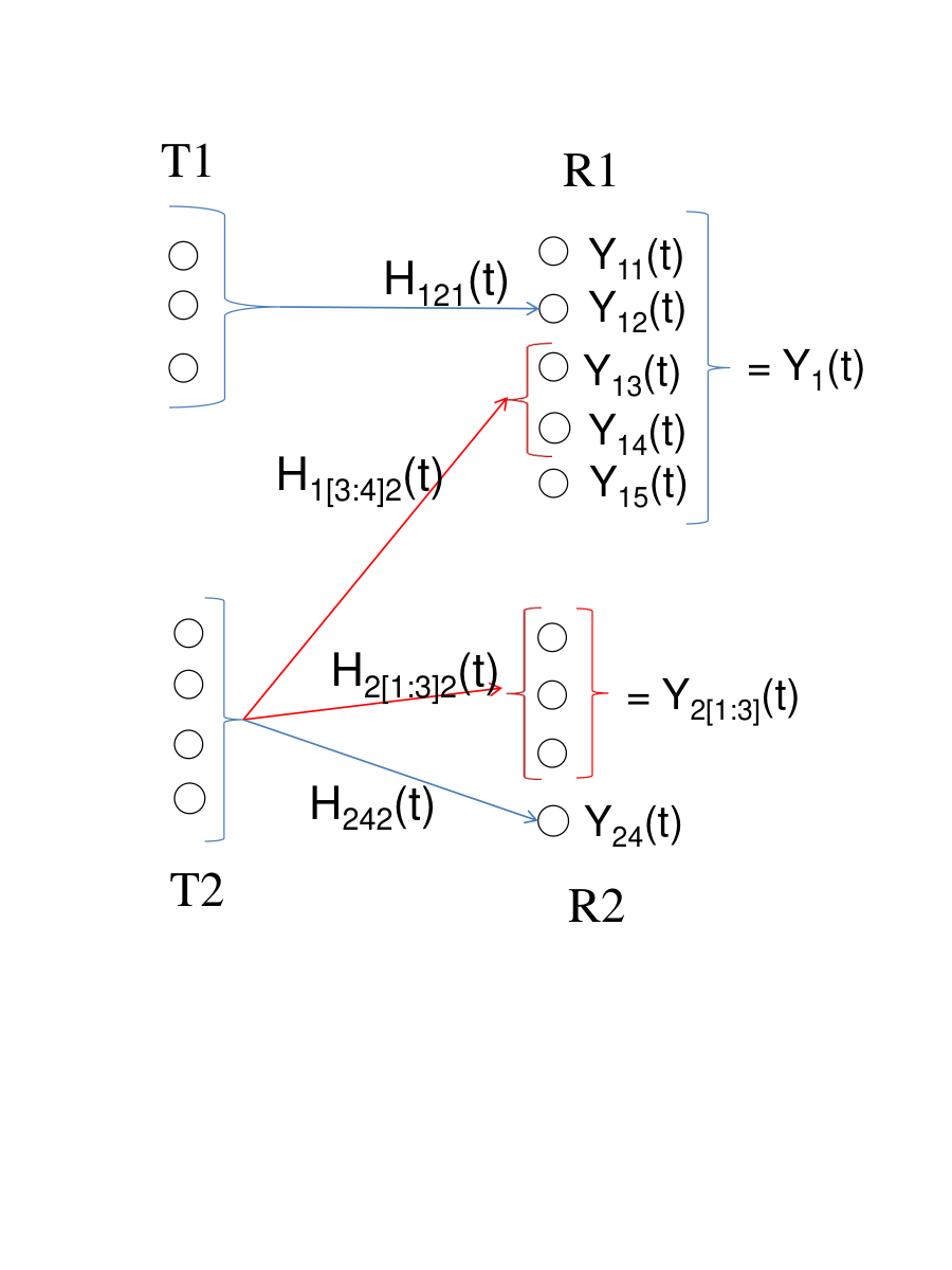
=\displaystyle= I(ℳ1;Y¯1(n),Y¯2(n)|ℳ2,H¯(n))+nϵn\displaystyle I\Big(\mathcal{M}_{1};\overline{Y}_{1}(n),\overline{Y}_{2}(n)\Big|\mathcal{M}_{2},\overline{H}(n)\Big)+n\epsilon_{n}
=\displaystyle= ∑t=1nh(Y1(t),Y2(t)|Y¯1(t−1),Y¯2(t−1),ℳ2,H¯(n))\displaystyle\sum_{t=1}^{n}h\Big(Y_{1}(t),Y_{2}(t)\Big|\overline{Y}_{1}(t-1),\overline{Y}_{2}(t-1),\mathcal{M}_{2},\overline{H}(n)\Big)
−∑t=1nh(Y1(t),Y2(t)|Y¯1(t−1),Y¯2(t−1),ℳ2,ℳ1,H¯(n))+nϵn\displaystyle-\sum_{t=1}^{n}h\Big(Y_{1}(t),Y_{2}(t)\Big|\overline{Y}_{1}(t-1),\overline{Y}_{2}(t-1),\mathcal{M}_{2},\mathcal{M}_{1},\overline{H}(n)\Big)+n\epsilon_{n} (9)
=\displaystyle= ∑t=1nh(Y1(t),Y2(t)|Y¯1(t−1),Y¯2(t−1),ℳ2,X¯2(t),H¯(n))\displaystyle\sum_{t=1}^{n}h\Big(Y_{1}(t),Y_{2}(t)\Big|\overline{Y}_{1}(t-1),\overline{Y}_{2}(t-1),\mathcal{M}_{2},\overline{X}_{2}(t),\overline{H}(n)\Big)
−∑t=1nh(Y1(t),Y2(t)|Y¯1(t−1),Y¯2(t−1),ℳ2,ℳ1,X¯1(t),X¯2(t),H¯(n))+nϵn\displaystyle-\sum_{t=1}^{n}h\Big(Y_{1}(t),Y_{2}(t)\Big|\overline{Y}_{1}(t-1),\overline{Y}_{2}(t-1),\mathcal{M}_{2},\mathcal{M}_{1},\overline{X}_{1}(t),\overline{X}_{2}(t),\overline{H}(n)\Big)+n\epsilon_{n} (10)
=\displaystyle= ∑t=1nh(Y1(t),Y2(t)|Y¯1(t−1),Y¯2(t−1),ℳ2,X¯2(t),H¯(t))\displaystyle\sum_{t=1}^{n}h\Big(Y_{1}(t),Y_{2}(t)\Big|\overline{Y}_{1}(t-1),\overline{Y}_{2}(t-1),\mathcal{M}_{2},\overline{X}_{2}(t),\overline{H}(t)\Big)
−∑t=1nh(Y1(t),Y2(t)|Y¯1(t−1),Y¯2(t−1),ℳ2,ℳ1,X¯1(t),X¯2(t),H¯(t))+nϵn\displaystyle-\sum_{t=1}^{n}h\Big(Y_{1}(t),Y_{2}(t)\Big|\overline{Y}_{1}(t-1),\overline{Y}_{2}(t-1),\mathcal{M}_{2},\mathcal{M}_{1},\overline{X}_{1}(t),\overline{X}_{2}(t),\overline{H}(t)\Big)+n\epsilon_{n} (11)
=\displaystyle= ∑t=1nh(Y1(t),Y2(t)|Y¯1(t−1),Y¯2(t−1),ℳ2,X¯2(t),H¯(t))\displaystyle\sum_{t=1}^{n}h\Big(Y_{1}(t),Y_{2}(t)\Big|\overline{Y}_{1}(t-1),\overline{Y}_{2}(t-1),\mathcal{M}_{2},\overline{X}_{2}(t),\overline{H}(t)\Big)
−∑t=1nh(W1(t),W2(t))+nϵn\displaystyle-\sum_{t=1}^{n}h\Big(W_{1}(t),W_{2}(t)\Big)+n\epsilon_{n} (12)
=\displaystyle= ∑t=1n{h(Y1(t),Y2(t)|Y¯1(t−1),Y¯2(t−1),ℳ2,X¯2(t)H¯(t))+o(log2P)+ϵn},\displaystyle\sum_{t=1}^{n}\left\{h\Big(Y_{1}(t),Y_{2}(t)\Big|\overline{Y}_{1}(t-1),\overline{Y}_{2}(t-1),\mathcal{M}_{2},\overline{X}_{2}(t)\overline{H}(t)\Big)+o(\log_{2}P)+\epsilon_{n}\right\}, (13)

where various steps follow because of the following reasons: the equality in (8) holds due to the independence of the two messages; equality (9) holds because of the definition of the mutual information and the chain rule for the differential entropy; equality (10) follows by noting that the transmit signal Xi​(t)X_{i}(t) is a deterministic function of ℳi\mathcal{M}_{i}, Y¯1​(t−1)\overline{Y}_{1}(t-1), Y¯2​(t−1)\overline{Y}_{2}(t-1), and H¯​(t)\overline{H}(t); (11) holds since all the involved random variables are independent of H([t+1:n])H([t+1:n]); (12) holds because translation does not change differential entropy, and W1​(t)W_{1}(t) and W2​(t)W_{2}(t) are independent of Y¯1​(t−1)\overline{Y}_{1}(t-1), Y¯2​(t−1)\overline{Y}_{2}(t-1), ℳ2\mathcal{M}_{2}, ℳ1\mathcal{M}_{1}, X¯1​(t)\overline{X}_{1}(t), X¯2​(t)\overline{X}_{2}(t), and H¯​(t)\overline{H}(t); the final equality holds since the noises are i.i.d. across time and their statistics are independent of PP.

Lemma 2

Let m1=△min⁡(M1,N1+N2)m_{1}\stackrel{{\scriptstyle\triangle}}{{=}}\min(M_{1},N_{1}+N_{2}) and m2=△min⁡(M1,N2)m_{2}\stackrel{{\scriptstyle\triangle}}{{=}}\min(M_{1},N_{2}). Then, for each t∈[1:n]t\in[1:n], we have

1m2​h​(Y2​(t)|Y¯2​(t−1),ℳ2,X¯2​(t),H¯​(t))\displaystyle\frac{1}{m_{2}}h\Big(Y_{2}(t)\Big|\overline{Y}_{2}(t-1),\mathcal{M}_{2},\overline{X}_{2}(t),\overline{H}(t)\Big)
≥1m1h(Y1(t),Y2(t)|Y¯1(t−1),Y¯2(t−1),ℳ2,X¯2(t),H¯(t))+o(log2P)\displaystyle{}\geq\frac{1}{m_{1}}h\Big(Y_{1}(t),Y_{2}(t)\Big|\overline{Y}_{1}(t-1),\overline{Y}_{2}(t-1),\mathcal{M}_{2},\overline{X}_{2}(t),\overline{H}(t)\Big)+o(\log_{2}P)

where the term o⁡(log2⁡P)o(\log_{2}P) is constant with nn.

Proof:

See Section III-A. ∎

Combining the bounds in (7), (13), and the one in Lemma 2, we get

1m2​R2\displaystyle\frac{1}{m_{2}}R_{2} ≤\displaystyle\leq 1m2⋅n​h​(Y¯2​(n)|H¯​(n))+ϵnm2−{1m1​R1−o⁡(log2⁡P)−ϵn}\displaystyle\frac{1}{m_{2}\cdot n}h\Big(\overline{Y}_{2}(n)\Big|\overline{H}(n)\Big)+\frac{\epsilon_{n}}{m_{2}}-\left\{\frac{1}{m_{1}}R_{1}-o(\log_{2}P)-\epsilon_{n}\right\}
⇒R2m2+R1m1\displaystyle\Rightarrow\frac{R_{2}}{m_{2}}+\frac{R_{1}}{m_{1}} ≤\displaystyle\leq min⁡(N2,M1+M2)m2⋅log2⁡P+ϵn​(1m2+1)+o⁡(log2⁡P),\displaystyle\frac{\min(N_{2},M_{1}+M_{2})}{m_{2}}\cdot\log_{2}P+\epsilon_{n}\left(\frac{1}{m_{2}}+1\right)+o(\log_{2}P),

where the last inequality holds since the DoF of the point-to-point MIMO channel are equal to the minimum of the number of transmit and receive antennas. Since ϵn→0\epsilon_{n}\to 0 as n→∞n\to\infty, we now have

R2m2+R1m1\displaystyle\frac{R_{2}}{m_{2}}+\frac{R_{1}}{m_{1}} ≤\displaystyle\leq min⁡(N2,M1+M2)m2⋅log2⁡P+o⁡(log2⁡P)\displaystyle\frac{\min(N_{2},M_{1}+M_{2})}{m_{2}}\cdot\log_{2}P+o(\log_{2}P)
⇒d2m2+d1m1\displaystyle\Rightarrow\frac{d_{2}}{m_{2}}+\frac{d_{1}}{m_{1}} ≤\displaystyle\leq lim supP→∞R2m2+R1m1≤min⁡(N2,M1+M2)m2\displaystyle\limsup_{P\to\infty}\frac{R_{2}}{m_{2}}+\frac{R_{1}}{m_{1}}\leq\frac{\min(N_{2},M_{1}+M_{2})}{m_{2}}

as desired.

III-A Proof of Lemma 2

In the following two lemmas, it is shown that although the received signals Y1​(t)Y_{1}(t) and Y2​(t)Y_{2}(t) are N1N_{1} and N2N_{2} dimensional, respectively, only the first m1−m2m_{1}-m_{2} and m2m_{2} entries of them are relevant as far as the current DoF analysis is concerned.

Lemma 3

If m2=min⁡(M1,N2)m_{2}=\min(M_{1},N_{2}), we have the following:

h(Y2(t)|Y¯2(t−1),ℳ2,X¯2(t),H¯(t))≥h(Y2[1:m2](t)|Y¯2(t−1),ℳ2,X¯2(t),H¯(t))+o(log2P),h\Big(Y_{2}(t)\Big|\overline{Y}_{2}(t-1),\mathcal{M}_{2},\overline{X}_{2}(t),\overline{H}(t)\Big)\geq h\Big(Y_{2[1:m_{2}]}(t)\Big|\overline{Y}_{2}(t-1),\mathcal{M}_{2},\overline{X}_{2}(t),\overline{H}(t)\Big)+o(\log_{2}P),

where the term o⁡(log2⁡P)o(\log_{2}P) is constant with nn.

Proof:

Follows from the techniques in [20, Proof of Lemma 2]. ∎

Lemma 4

If m1=min⁡(M1,N1+N2)m_{1}=\min(M_{1},N_{1}+N_{2}), then

h(Y1(t),Y2(t)|Y¯1(t−1),Y¯2(t−1),ℳ2,X¯2(t),H¯(t))\displaystyle h\Big(Y_{1}(t),Y_{2}(t)\Big|\overline{Y}_{1}(t-1),\overline{Y}_{2}(t-1),\mathcal{M}_{2},\overline{X}_{2}(t),\overline{H}(t)\Big)
≤h(Y1[1:m1−m2](t),Y2[1:m2](t)|Y¯1(t−1),Y¯2(t−1),ℳ2,X¯2(t),H¯(t))+o(log2P).\displaystyle{}\leq h\Big(Y_{1[1:m_{1}-m_{2}]}(t),Y_{2[1:m_{2}]}(t)\Big|\overline{Y}_{1}(t-1),\overline{Y}_{2}(t-1),\mathcal{M}_{2},\overline{X}_{2}(t),\overline{H}(t)\Big)+o(\log_{2}P).

where the term o⁡(log2⁡P)o(\log_{2}P) is constant with nn.

Proof:

Follows from the techniques in [20, Proof of Lemma 3]. ∎

If m1−m2=0m_{1}-m_{2}=0, Lemma 2 holds trivially. Hence, in the following, we may consider without loss of generality that m1>m2m_{1}>m_{2}.

We now prove the following lemma which is critical in the proof of Lemma 2.

Lemma 5

Let Q⁡(t)=△{ℳ2,H¯​(t),Y¯2​(t−1),X¯2​(t)}Q(t)\stackrel{{\scriptstyle\triangle}}{{=}}\big\{\mathcal{M}_{2},\overline{H}(t),\overline{Y}_{2}(t-1),\overline{X}_{2}(t)\big\}. For an i∈[1:m2−1]i\in[1:m_{2}-1] and a k∈[1:m1−m2]k\in[1:m_{1}-m_{2}], if j=i+1j=i+1 and l=k+1l=k+1, we have the following equalities:

h(Y2​i(t)|Q(t),Y2[1:i−1](t))\displaystyle h\Big(Y_{2i}(t)\Big|Q(t),Y_{2[1:i-1]}(t)\Big) =\displaystyle= h(Y2​j(t)|Q(t),Y2[1:i−1](t));\displaystyle h\Big(Y_{2j}(t)\Big|Q(t),Y_{2[1:i-1]}(t)\Big);
h(Y2​m2(t)|Q(t),Y2[1:m2−1](t))\displaystyle h\Big(Y_{2m_{2}}(t)\Big|Q(t),Y_{2[1:m_{2}-1]}(t)\Big) =\displaystyle= h(Y11(t)|Q(t),Y2[1:m2−1](t));\displaystyle h\Big(Y_{11}(t)\Big|Q(t),Y_{2[1:m_{2}-1]}(t)\Big);
h(Y1​k(t)|Q(t),Y2[1:m2](t),Y1[1:k−1](t))\displaystyle h\Big(Y_{1k}(t)\Big|Q(t),Y_{2[1:m_{2}]}(t),Y_{1[1:k-1]}(t)\Big) =\displaystyle= h(Y1​l(t)|Q(t),Y2[1:m2](t),Y1[1:k−1](t)).\displaystyle h\Big(Y_{1l}(t)\Big|Q(t),Y_{2[1:m_{2}]}(t),Y_{1[1:k-1]}(t)\Big).
Proof:

It is sufficient to prove the first equality. Define Y2′​(t)=Y2​(t)−H22​(t)​X2​(t)=H21​(t)​X1​(t)+W2​(t)Y_{2}^{\prime}(t)=Y_{2}(t)-H_{22}(t)X_{2}(t)=H_{21}(t)X_{1}(t)+W_{2}(t).

Toward this end, we have the following sequence of equalities,

h(Y2​i(t)|Q(t),Y2[1:i−1](t))\displaystyle h\Big(Y_{2i}(t)\Big|Q(t),Y_{2[1:i-1]}(t)\Big) (14)
=h(Y2​i(t)|ℳ2,H¯(t),Y¯2(t−1),X¯2(t),Y2[1:i−1](t))\displaystyle{}\hskip-34.14322pt=h\Big(Y_{2i}(t)\Big|\mathcal{M}_{2},\overline{H}(t),\overline{Y}_{2}(t-1),\overline{X}_{2}(t),Y_{2[1:i-1]}(t)\Big)
=h(Y2​i′(t)|ℳ2,H¯(t−1),Y¯2(t−1),X¯2(t),Y2[1:i−1]′(t),H2[1:i]1(t),H11(t),H12(t),H22(t),H2[i+1:N2]1(t))\displaystyle{}\hskip-34.14322pt=h\Big(Y_{2i}^{\prime}(t)\Big|\mathcal{M}_{2},\overline{H}(t-1),\overline{Y}_{2}(t-1),\overline{X}_{2}(t),Y_{2[1:i-1]}^{\prime}(t),H_{2[1:i]1}(t),H_{11}(t),H_{12}(t),H_{22}(t),H_{2[i+1:N_{2}]1}(t)\Big) (15)
=h(Y2​i′(t)|ℳ2,H¯(t−1),Y¯2(t−1),X¯2(t),Y2[1:i−1]′(t),H2[1:i]1(t))\displaystyle{}\hskip-34.14322pt=h\Big(Y_{2i}^{\prime}(t)\Big|\mathcal{M}_{2},\overline{H}(t-1),\overline{Y}_{2}(t-1),\overline{X}_{2}(t),Y_{2[1:i-1]}^{\prime}(t),H_{2[1:i]1}(t)\Big) (16)
=𝔼H2​i​1​(t)=ah(Y2​i′(t)|ℳ2,H¯(t−1),Y¯2(t−1),X¯2(t),Y2[1:i−1]′(t),H2[1:i−1]1(t),H2​i​1(t)=a)\displaystyle{}\hskip-34.14322pt=\mathbb{E}_{H_{2i1}(t)=a}~h\Big(Y_{2i}^{\prime}(t)\Big|\mathcal{M}_{2},\overline{H}(t-1),\overline{Y}_{2}(t-1),\overline{X}_{2}(t),Y_{2[1:i-1]}^{\prime}(t),H_{2[1:i-1]1}(t),H_{2i1}(t)=a\Big) (17)
=𝔼H2​j​1​(t)=ah(Y2​j′(t)|ℳ2,H¯(t−1),Y¯2(t−1),X¯2(t),Y2[1:i−1]′(t),H2[1:i−1]1(t),H2​j​1(t)=a)\displaystyle{}\hskip-34.14322pt=\mathbb{E}_{H_{2j1}(t)=a}~h\Big(Y_{2j}^{\prime}(t)\Big|\mathcal{M}_{2},\overline{H}(t-1),\overline{Y}_{2}(t-1),\overline{X}_{2}(t),Y_{2[1:i-1]}^{\prime}(t),H_{2[1:i-1]1}(t),H_{2j1}(t)=a\Big) (18)
=h(Y2​j′(t)|ℳ2,H¯(t−1),Y¯2(t−1),X¯2(t),Y2[1:i−1]′(t),H2[1:i−1]1(t),H2​j​1(t))\displaystyle{}\hskip-34.14322pt=h\Big(Y_{2j}^{\prime}(t)\Big|\mathcal{M}_{2},\overline{H}(t-1),\overline{Y}_{2}(t-1),\overline{X}_{2}(t),Y_{2[1:i-1]}^{\prime}(t),H_{2[1:i-1]1}(t),H_{2j1}(t)\Big) (19)
=h(Y2​j(t)|ℳ2,H¯(t−1),Y¯2(t−1),X¯2(t),Y2[1:i−1](t),H(t)),\displaystyle{}\hskip-34.14322pt=h\Big(Y_{2j}(t)\Big|\mathcal{M}_{2},\overline{H}(t-1),\overline{Y}_{2}(t-1),\overline{X}_{2}(t),Y_{2[1:i-1]}(t),H(t)\Big), (20)

where the various equalities hold as follows: (14) holds by the definition of Q⁡(t)Q(t); (15) holds because translation does not change differential entropy [1]; (16) follows by noting that {H11(t),H12(t),H22(t),H2[i+1:N2]1(t)}\big\{H_{11}(t),H_{12}(t),H_{22}(t),H_{2[i+1:N_{2}]1}(t)\big\} are independent of {Y2​i′(t),ℳ2,H¯(t−1),Y¯2(t−1),X¯2(t),Y2[1:i−1]′(t),H2[1:i]1(t)}\big\{Y_{2i}^{\prime}(t),\mathcal{M}_{2},\overline{H}(t-1),\overline{Y}_{2}(t-1),\overline{X}_{2}(t),Y_{2[1:i-1]}^{\prime}(t),H_{2[1:i]1}(t)\big\} (note the present channel matrices are independent of the present and the past channel inputs and noises); (17) holds by the definition of the conditional differential entropy; (18) holds because conditioned on {ℳ2,H¯(t−1),Y¯2(t−1),X¯2(t),Y2[1:i−1]′(t),H2[1:i−1]1(t)}\big\{\mathcal{M}_{2},\overline{H}(t-1),\overline{Y}_{2}(t-1),\overline{X}_{2}(t),Y_{2[1:i-1]}^{\prime}(t),H_{2[1:i-1]1}(t)\big\}, the joint distribution of {H2​i​1​(t),X1​(t),W2​i​(t)}\big\{H_{2i1}(t),X_{1}(t),W_{2i}(t)\big\} is identical to that of {H2​j​1​(t),X1​(t),W2​j​(t)}\big\{H_{2j1}(t),X_{1}(t),W_{2j}(t)\big\}; (19) holds by the definition of the conditional differential entropy; (20) holds since {H2​i​1(t),H2[i+2:N2]1(t),H11(t),H12(t),H22(t)}\big\{H_{2i1}(t),H_{2[i+2:N_{2}]1}(t),H_{11}(t),H_{12}(t),H_{22}(t)\big\} are independent of {Y2​j′(t),ℳ2,H¯(t−1),Y¯2(t−1),X¯2(t),Y2[1:i−1]′(t),H2[1:i−1]1(t),H2​j​1(t)}\big\{Y_{2j}^{\prime}(t),\mathcal{M}_{2},\overline{H}(t-1),\overline{Y}_{2}(t-1),\overline{X}_{2}(t),Y_{2[1:i-1]}^{\prime}(t),H_{2[1:i-1]1}(t),H_{2j1}(t)\big\} and since translation does not change differential entropy. ∎

Note that the first equality in the above lemma asserts that the signals Y2​i​(t)Y_{2i}(t) and Y2​j​(t)Y_{2j}(t) received at the it​hi^{th} and jt​hj^{th} antenna, respectively, of R2 have equal differential entropy, when conditioned on the channel matrices H¯​(t)\overline{H}(t), the message ℳ2\mathcal{M}_{2} and the transmit signal X¯2​(t)\overline{X}_{2}(t) of T2, the past channel outputs Y¯2​(t−1)\overline{Y}_{2}(t-1), and the present channel outputs Y2[1:i−1](t)Y_{2[1:i-1]}(t) at some other receive antennas. We refer to this property as the statistical equivalence of the channel outputs, which essentially says that given the past and present channel outputs, the signals received at any two antennas of the system provide an equal amount of information about ℳ1\mathcal{M}_{1}. Note that this property of statistical equivalence of the channel outputs was shown to hold in [20] for the case of delayed CSIT. Here, on the other hand, the same property is shown to be true under the stronger setting of Shannon feedback.

The above lemma yields the following simple corollary, where Q⁡(t)={ℳ2,H¯​(t),Y¯2​(t−1),X¯2​(t)}Q(t)=\big\{\mathcal{M}_{2},\overline{H}(t),\overline{Y}_{2}(t-1),\overline{X}_{2}(t)\big\} as before.

Corollary 3

For an i∈[1:m2−1]i\in[1:m_{2}-1] and a k∈[1:m1−m2]k\in[1:m_{1}-m_{2}], if j=i+1j=i+1 and l=k+1l=k+1, we have the following:

h(Y2​i(t)|Q(t),Y2[1:i−1](t))\displaystyle h\Big(Y_{2i}(t)\Big|Q(t),Y_{2[1:i-1]}(t)\Big) ≥\displaystyle\geq h(Y2​j(t)|Q(t),Y2[1:i](t));\displaystyle h\Big(Y_{2j}(t)\Big|Q(t),Y_{2[1:i]}(t)\Big);
h(Y2​m2(t)|Q(t),Y2[1:m2−1](t))\displaystyle h\Big(Y_{2m_{2}}(t)\Big|Q(t),Y_{2[1:m_{2}-1]}(t)\Big) ≥\displaystyle\geq h(Y11(t)|Q(t),Y2[1:m2](t));\displaystyle h\Big(Y_{11}(t)\Big|Q(t),Y_{2[1:m_{2}]}(t)\Big);
h(Y1​k(t)|Q(t),Y2[1:m2](t),Y1[1:k−1](t))\displaystyle h\Big(Y_{1k}(t)\Big|Q(t),Y_{2[1:m_{2}]}(t),Y_{1[1:k-1]}(t)\Big) ≥\displaystyle\geq h(Y1​l(t)|Q(t),Y2[1:m2](t),Y1[1:k](t)).\displaystyle h\Big(Y_{1l}(t)\Big|Q(t),Y_{2[1:m_{2}]}(t),Y_{1[1:k]}(t)\Big).
Proof:

Follows from the previous lemma by invoking the fact that conditioning reduces entropy [1]. ∎

Lemma 6

We have

m1⋅h(Y2[1:m2](t)|Q(t))≥m2⋅h(Y1[1:m1−m2](t),Y2[1:m2](t)|Q(t),Y¯1(t−1)).m_{1}\cdot h\Big(Y_{2[1:m_{2}]}(t)\Big|Q(t)\Big)\geq m_{2}\cdot h\Big(Y_{1[1:m_{1}-m_{2}]}(t),Y_{2[1:m_{2}]}(t)\Big|Q(t),\overline{Y}_{1}(t-1)\Big).
Proof:

By the previous corollary and the chain rule for the differential entropy, we get

1m2h(Y2[1:m2](t)|Q(t))=1m2∑i=1m2h(Y2​i(t)|Q(t),Y2[1:i−1](t))\displaystyle\frac{1}{m_{2}}h\Big(Y_{2[1:m_{2}]}(t)\Big|Q(t)\Big)=\frac{1}{m_{2}}\sum_{i=1}^{m_{2}}h\Big(Y_{2i}(t)\Big|Q(t),Y_{2[1:i-1]}(t)\Big)
≥h(Y2​m2(t)|Q(t),Y2[1:m2−1](t))\displaystyle{}\geq h\Big(Y_{2m_{2}}(t)\Big|Q(t),Y_{2[1:m_{2}-1]}(t)\Big)
≥h(Y11(t)|Q(t),Y2[1:m2](t))\displaystyle{}\geq h\Big(Y_{11}(t)\Big|Q(t),Y_{2[1:m_{2}]}(t)\Big)
≥1m1−m2h(Y1[1:m1−m2](t)|Q(t),Y2[1:m2](t)).\displaystyle{}\geq\frac{1}{m_{1}-m_{2}}h\Big(Y_{1[1:m_{1}-m_{2}]}(t)\Big|Q(t),Y_{2[1:m_{2}]}(t)\Big).

This yields

(m1−m2)⋅h(Y2[1:m2](t)|Q(t))\displaystyle(m_{1}-m_{2})\cdot h\Big(Y_{2[1:m_{2}]}(t)\Big|Q(t)\Big) ≥\displaystyle\geq m2⋅h(Y1[1:m1−m2](t)|Q(t),Y2[1:m2](t))\displaystyle m_{2}\cdot h\Big(Y_{1[1:m_{1}-m_{2}]}(t)\Big|Q(t),Y_{2[1:m_{2}]}(t)\Big) (21)
≥\displaystyle\geq m2⋅h(Y1[1:m1−m2](t)|Q(t),Y¯1(t−1),Y2[1:m2](t))\displaystyle m_{2}\cdot h\Big(Y_{1[1:m_{1}-m_{2}]}(t)\Big|Q(t),\overline{Y}_{1}(t-1),Y_{2[1:m_{2}]}(t)\Big)

since conditioning reduces entropy. Similarly, we can obtain

m2⋅h(Y2[1:m2](t)|Q(t))≥m2⋅h(Y2[1:m2](t)|Q(t),Y¯1(t−1)).\displaystyle m_{2}\cdot h\Big(Y_{2[1:m_{2}]}(t)\Big|Q(t)\Big)\geq m_{2}\cdot h\Big(Y_{2[1:m_{2}]}(t)\Big|Q(t),\overline{Y}_{1}(t-1)\Big). (22)

The lemma can now be obtained by adding the inequalities in (21) and (22). ∎

The inequality in Lemma 2 can now be derived by combining the results of Lemmas 3, 4, and 6, and by noting that the sum or the difference of two o⁡(log2⁡P)o(\log_{2}P) terms yields another o⁡(log2⁡P)o(\log_{2}P) term.

IV Proof of Theorem 2

As mentioned before, it is sufficient to prove that the outer-bound 𝐃outerS\mathbf{D}^{\rm S}_{\rm outer} is achievable when Condition 11 holds. Throughout this section, it is assumed that Condition 11 holds.

Here, bound L2L_{2} can be easily shown to be redundant (it is implied by L3L_{3}), and thus can be ignored. Further, in the present case, bounds L1L_{1} and L3L_{3} are given by

L1≡d1M1′+d2N2≤1​ and ​L3≡d1+d2≤N1,L_{1}\equiv\frac{d_{1}}{M_{1}^{\prime}}+\frac{d_{2}}{N_{2}}\leq 1~\mbox{ and }~L_{3}\equiv d_{1}+d_{2}\leq N_{1},

where M1′=△min⁡(M1,N1+N2)M_{1}^{\prime}\stackrel{{\scriptstyle\triangle}}{{=}}\min(M_{1},N_{1}+N_{2}).

Fig. 9: Two Possible Shapes of the Outer-Bound when Condition 11 Holds

The typical shape of the outer-bound is shown in Fig. 9, where Po​2,1P_{o2,1} is the point of intersection of the line d2=M2d_{2}=M_{2} and the one corresponding to bound L1L_{1}, similarly Po​2,3P_{o2,3}, and P1,3P_{1,3} is the point of intersection of lines corresponding to bounds L1L_{1} and L3L_{3}. Moreover,

P02,1≡(M1′​N2−M2N2,M2),P1,3≡(M1′​N1−N2M1′−N2,N2​M1′−N1M1′−N2), and ​Po​2,3≡(N1−M2,M2).P_{02,1}\equiv\left(M_{1}^{\prime}\frac{N_{2}-M_{2}}{N_{2}},M_{2}\right),~\!P_{1,3}\equiv\left(M_{1}^{\prime}\frac{N_{1}-N_{2}}{M_{1}^{\prime}-N_{2}},N_{2}\frac{M_{1}^{\prime}-N_{1}}{M_{1}^{\prime}-N_{2}}\right),\mbox{ and }P_{o2,3}\equiv(N_{1}-M_{2},M_{2}).

Depending on whether the d2d_{2}-coordinate of P1,3P_{1,3} is less than M2M_{2} or not, we have to consider two cases separately.
∙Case A: M1′≥N2N1−M2N2−M2:¯\bullet~\underline{\mbox{Case A: }M_{1}^{\prime}\geq N_{2}\frac{N_{1}-M_{2}}{N_{2}-M_{2}}~:}

Here, bound L1L_{1} is redundant. Moreover, from Fig. 9, one may observe that if Po​2,3∈𝐃SP_{o2,3}\in\mathbf{D}^{\rm S} then 𝐃outerS=𝐃S\mathbf{D}^{\rm S}_{\rm outer}=\mathbf{D}^{\rm S}. Hence, we find here sufficient to prove that Po​2,3∈𝐃SP_{o2,3}\in\mathbf{D}^{\rm S}.
∙Case B: M1′<N2N1−M2N2−M2:¯\bullet~\underline{\mbox{Case B: }M_{1}^{\prime}<N_{2}\frac{N_{1}-M_{2}}{N_{2}-M_{2}}~:}

Here, bounds L1L_{1} and L3L_{3} are both active. From Fig. 9, we observe the sufficiency of proving that Po​2,1,P1,3∈𝐃SP_{o2,1},P_{1,3}\in\mathbf{D}^{\rm S}.

Next, we propose a generic retrospective interference alignment scheme, which is used later to prove that Po​2,3∈𝐃SP_{o2,3}\in\mathbf{D}^{\rm S} under Case A and Po​2,1,P1,3∈𝐃SP_{o2,1},P_{1,3}\in\mathbf{D}^{\rm S} under Case B with an appropriate choice of parameters. This scheme is specified in terms of the parameters

T,t1,t2,{m1​(i)}i=1T, and ​{m2​(i)}i=1T,T,~t_{1},~t_{2},~\Big\{m_{1}(i)\Big\}_{i=1}^{T},~\mbox{ and }~\Big\{m_{2}(i)\Big\}_{i=1}^{T}, (23)

where T,t1,t2∈ℕT,t_{1},t_{2}\in\mathbb{N}, m1​(i),m2​(i)∈ℕ∪{0}m_{1}(i),m_{2}(i)\in\mathbb{N}\cup\{0\} ∀\forall ii, and Design Criteria 1-5, which are stated in the sequel. It is developed such that if, for a given a DoF pair P≡(d1,d2)P\equiv(d_{1},d_{2}) and the given (M1,M2,N1,N2)(M_{1},M_{2},N_{1},N_{2}) MIMO IC, the parameters in (23) can be chosen as functions of (d1,d2)(d_{1},d_{2}) and (M1,M2,N1,N2)(M_{1},M_{2},N_{1},N_{2}) so that Design Criteria 1-5 are satisfied, then the DoF pair P≡(d1,d2)∈𝐃SP\equiv(d_{1},d_{2})\in\mathbf{D}^{\rm S} of the given (M1,M2,N1,N2)(M_{1},M_{2},N_{1},N_{2}) MIMO IC.

Consider now the retrospective interference alignment scheme. The goal is to prove that a given DoF pair P≡(d1,d2)∈𝐃SP\equiv(d_{1},d_{2})\in\mathbf{D}^{\rm S}. Let us first state two important design criteria.

Design Criterion 1

Choose positive integers t1t_{1} and t2t_{2} such that t1+t2=Tt_{1}+t_{2}=T.

Design Criterion 2

Choose a positive integer TT such that T​d1Td_{1} and T​d2Td_{2} are integers.

Now, choose a B∈ℕB\in\mathbb{N} and set

T⋆=(B+1)⋅T,di⋆=B⋅T⋅di, where ​i∈{1,2}, and ​P⋆≡(d1⋆T⋆,d1⋆T⋆)=(d11+1B,d21+1B).\displaystyle T^{\star}=(B+1)\cdot T,~d_{i}^{\star}=B\cdot T\cdot d_{i},\mbox{ where }i\in\{1,2\},~\mbox{ and }P^{\star}\equiv\left(\frac{d_{1}^{\star}}{T^{\star}},\frac{d_{1}^{\star}}{T^{\star}}\right)=\left(\frac{d_{1}}{1+\tfrac{1}{B}},\frac{d_{2}}{1+\tfrac{1}{B}}\right).

It will be proved that for any positive integer BB, by coding over T⋆T^{\star} time slots, we can simultaneously achieve d1⋆d_{1}^{\star} and d2⋆d_{2}^{\star} DoF for the two users respectively. This implies that P∈𝐃SP\in\mathbf{D}^{\rm S}, since the DoF region is closed, and the point P⋆P^{\star} converges to PP as B→∞B\to\infty. Thus, our aim in the following is to prove the achievability of point P⋆P^{\star}.

The entire duration of T⋆T^{\star} is divided into B+1B+1 blocks, each consisting of TT time slots. Each block is further divided into two phases with Phase One having t1t_{1} time slots and Phase Two the remainder of t2=T−t1t_{2}=T-t_{1} time slots.

Definition 3

Define two functions b⁡(t)b(t), the index of the block to which time slot tt belongs, and t¯​(t)\overline{t}(t), the index of that time slot within Block b⁡(t)b(t), as

b⁡(t)=⌈tT⌉ and t¯​(t)=t−T⋅(b⁡(t)−1).b(t)=\left\lceil\frac{t}{T}\right\rceil\quad\mbox{ and }\quad\overline{t}(t)=t-T\cdot\big(b(t)-1\big).

Note that t¯(t)∈[1:T]\overline{t}(t)\in[1:T]. Thus, each time slot tt can be uniquely identified by the pair (b​(t),t¯​(t))\big(b(t),\overline{t}(t)\big). Block bb, b∈[1:B+1]b\in[1:B+1], consists of time slots t∈[b′T+1:b′T+T]t\in[b^{\prime}T+1:b^{\prime}T+T], where b′=△b−1b^{\prime}\stackrel{{\scriptstyle\triangle}}{{=}}b-1; we let Phase One of block bb consist of time slots t∈[b′T+1:b′T+t1]t\in[b^{\prime}T+1:b^{\prime}T+t_{1}] and Phase Two the remaining time slots t∈[b′T+t1+1:b′T+t1+t2]t\in[b^{\prime}T+t_{1}+1:b^{\prime}T+t_{1}+t_{2}].

The general structure of our achievability scheme has the following features:

  • •

    In each of the first BB blocks, T1 and T2 respectively transmit T​d1Td_{1} and T​d2Td_{2} i.i.d. complex Gaussian data symbols (DSs) intended for R1 and R2, respectively. In Block B+1B+1, no new DS is sent.

  • •

    In each time slot, T2 transmits an appropriate number of new DSs intended for R2, and therefore, in some sense, it does not play an active role in aligning interference (as in the example of Section II-C).

  • •

    T1, on the other hand, transmits all T​d1Td_{1} DSs, to be transmitted over a given block during Phase One of that block (time slots t=1t=1 or t=4t=4 constitute Phase One in the example of Section II-C). It signals over Phase Two such that at the end of each block, (a) R2 can decode all DSs sent to it over that block, and (b) R1 can decode all DSs sent to it over the previous block (note that t=2,3t=2,3 or t=4,5t=4,5 are counterparts of Phase Two in the example of Section II-C). To meet these objectives optimally, T1 needs to align interference at both receivers.

  • •

    Finally, the goal of Block B+1B+1 is to allow R1 to decode all DSs of Block BB by not sending any new data (Block B+1B+1, in some sense, corresponds to time slot t=7t=7 in the example of Section II-C).

Let T1 and T2 transmit m1​(i)m_{1}(i) and m2​(i)m_{2}(i) DSs intended for their respective receivers at the it​hi^{th} time slot of any given block (except, the last block) where these design parameters are chosen according to following criterion.

Design Criterion 3

Choose non-negative integers m1​(i)m_{1}(i) and m2​(i)m_{2}(i), i∈[1:T]i\in[1:T] , as follows.

  • •

    m1​(i)=0m_{1}(i)=0 ∀\forall i∈[t1+1:T]i\in[t_{1}+1:T] (recall, t1+t2=Tt_{1}+t_{2}=T);

  • •

    m1​(i)≤M1′m_{1}(i)\leq M_{1}^{\prime} ∀\forall i∈[1:t1]i\in[1:t_{1}] and ∑i=1Tm1​(i)=∑i=1t1m1​(i)=T​d1\sum_{i=1}^{T}m_{1}(i)=\sum_{i=1}^{t_{1}}m_{1}(i)=Td_{1};

  • •

    m2​(j)≤M2m_{2}(j)\leq M_{2} ∀\forall j∈[1:T]j\in[1:T] and ∑j=1Tm2​(j)=T​d2\sum_{j=1}^{T}m_{2}(j)=Td_{2}.

At time t∈[1:BT]t\in[1:BT], T1 transmits m1​(t¯​(t))m_{1}\big(\overline{t}(t)\big) complex Gaussian DSs, denoted by u1​i​(b⁡(t),t¯​(t))u_{1i}\big(b(t),\overline{t}(t)\big), whereas T2 transmits m2​(t¯​(t))m_{2}\big(\overline{t}(t)\big) complex Gaussian DSs, denoted by u2​i​(b⁡(t),t¯​(t))u_{2i}\big(b(t),\overline{t}(t)\big). Note that all DSs

{{{u1​i​(b,t¯)}i=1m1​(t¯)}t¯=1T}b=1B​and​{{{u2​j​(b,t¯)}j=1m2​(t¯)}t¯=1T}b=1B\left\{\Big\{\big\{u_{1i}(b,\overline{t})\big\}_{i=1}^{m_{1}(\overline{t})}\Big\}_{\overline{t}=1}^{T}\right\}_{b=1}^{B}~\mbox{and}~\left\{\Big\{\big\{u_{2j}(b,\overline{t})\big\}_{j=1}^{m_{2}(\overline{t})}\Big\}_{\overline{t}=1}^{T}\right\}_{b=1}^{B}

are i.i.d. Note that since m1​(i)=0m_{1}(i)=0 ∀\forall i∈[t1+1:t1+t2]i\in[t_{1}+1:t_{1}+t_{2}], no new DS is transmitted by T1 to R1 over Phase Two of any block so as to enable interference alignment and to ensure successful decoding.

The transmission scheme of T1 and T2 are described next. Focusing on Block bb, where b∈[1:B]b\in[1:B], the operation of T1 and T2 is described over the two phases separately. We start below with Phase One of Block bb. See also Tables I-III, where the main points about the operation of this scheme are summarized.

Block bb, Phase One: Here, t∈[b′T+1:b′T+t1]t\in[b^{\prime}T+1:b^{\prime}T+t_{1}] with b∈[1:B]b\in[1:B] and b′=b−1b^{\prime}=b-1. This phase is a data transmission phase.

At time t∈[b′T+1:b′T+t1]t\in[b^{\prime}T+1:b^{\prime}T+t_{1}] with b∈[1:B]b\in[1:B], T1 and T2 respectively transmit m1​(t¯​(t))m_{1}\big(\overline{t}(t)\big) and m2​(t¯​(t))m_{2}\big(\overline{t}(t)\big) DSs as follows:

X1​i​(t)\displaystyle X_{1i}(t) =\displaystyle= u1​i(b(t),t¯(t)),∀i∈[1:m1(t¯(t))], and\displaystyle u_{1i}\Big(b(t),\overline{t}(t)\Big),~\forall~\!i\in\Big[1:m_{1}\Big(\overline{t}(t)\Big)\Big],\mbox{ and}
X1​i​(t)\displaystyle X_{1i}(t) =\displaystyle= 0,∀i∈[m1(t¯(t))+1:M1]; and\displaystyle 0,~\forall~\!i\in\Big[m_{1}\Big(\overline{t}(t)\Big)+1:M_{1}\Big];\mbox{ and}
X2​j​(t)\displaystyle X_{2j}(t) =\displaystyle= u2​j(b(t),t¯(t)),∀j∈[1:m2(t¯(t))], and\displaystyle u_{2j}\Big(b(t),\overline{t}(t)\Big),~\forall~\!j\in\Big[1:m_{2}\Big(\overline{t}(t)\Big)\Big],\mbox{ and}
X2​j​(t)\displaystyle X_{2j}(t) =\displaystyle= 0,∀j∈[m2(t¯(t))+1:M2].\displaystyle 0,~\forall~\!j\in\Big[m_{2}\Big(\overline{t}(t)\Big)+1:M_{2}\Big].

Consider now the signals received by R1 and R2 during Phase One. Since we are interested in the achievability of the DoF, we ignore throughout the presence of additive noise since it can not affect a DoF result. Then for a t∈[b′T+1:b′T+t1]t\in[b^{\prime}T+1:b^{\prime}T+t_{1}] with b∈[1:B]b\in[1:B], we have

Y1​i​(t)\displaystyle Y_{1i}(t) =\displaystyle= H1​i​1(t)X1(t)+H1​i​2(t)X2(t)⋯i∈[1:N1]\displaystyle H_{1i1}(t)X_{1}(t)+H_{1i2}(t)X_{2}(t)~\cdots~i\in[1:N_{1}]
=\displaystyle= H1​i​1​(t)​[u11​(b​(t),t¯​(t))u12​(b​(t),t¯​(t))u1​m1​(t¯​(t))​(b⁡(t),t¯​(t))0[M1−m1​(t¯​(t))]×1]⏟=△LC1​i[1]​(b⁡(t),t¯​(t))+H1​i​2​(t)​[u21​(b​(t),t¯​(t))u22​(b​(t),t¯​(t))u2​m2​(t¯​(t))​(b⁡(t),t¯​(t))0[M2−m2​(t¯​(t))]×1]⏟=△LC1​i[2]​(b⁡(t),t¯​(t));\displaystyle\underbrace{H_{1i1}(t)\begin{bmatrix}u_{11}\left(b(t),\overline{t}(t)\right)\\ u_{12}\left(b(t),\overline{t}(t)\right)\\ \vdots\\ u_{1m_{1}\left(\overline{t}(t)\right)}\left(b(t),\overline{t}(t)\right)\\ 0_{\left[M_{1}-m_{1}\left(\overline{t}(t)\right)\right]\times 1}\end{bmatrix}}_{\stackrel{{\scriptstyle\triangle}}{{=}}~{\rm LC}_{1i}^{[1]}\left(b(t),\overline{t}(t)\right)}+\underbrace{H_{1i2}(t)\begin{bmatrix}u_{21}\left(b(t),\overline{t}(t)\right)\\ u_{22}\left(b(t),\overline{t}(t)\right)\\ \vdots\\ u_{2m_{2}\left(\overline{t}(t)\right)}\left(b(t),\overline{t}(t)\right)\\ 0_{\left[M_{2}-m_{2}\left(\overline{t}(t)\right)\right]\times 1}\end{bmatrix}}_{\stackrel{{\scriptstyle\triangle}}{{=}}~{\rm LC}_{1i}^{[2]}\left(b(t),\overline{t}(t)\right)};
Y2​j​(t)\displaystyle Y_{2j}(t) =\displaystyle= H2​j​1(t)X1(t)+H2​j​2(t)X2(t)⋯j∈[1:N2]\displaystyle H_{2j1}(t)X_{1}(t)+H_{2j2}(t)X_{2}(t)~\cdots~j\in[1:N_{2}]
=\displaystyle= H2​j​1​(t)​[u11​(b​(t),t¯​(t))u12​(b​(t),t¯​(t))u1​m1​(t¯​(t))​(b⁡(t),t¯​(t))0[M1−m1​(t¯​(t))]×1]⏟=△LC2​j[1]​(b⁡(t),t¯​(t))+H2​j​2​(t)​[u21​(b​(t),t¯​(t))u22​(b​(t),t¯​(t))u2​m2​(t¯​(t))​(b⁡(t),t¯​(t))0[M2−m2​(t¯​(t))]×1]⏟=△LC2​j[2]​(b⁡(t),t¯​(t)).\displaystyle\underbrace{H_{2j1}(t)\begin{bmatrix}u_{11}\left(b(t),\overline{t}(t)\right)\\ u_{12}\left(b(t),\overline{t}(t)\right)\\ \vdots\\ u_{1m_{1}\left(\overline{t}(t)\right)}\left(b(t),\overline{t}(t)\right)\\ 0_{\left[M_{1}-m_{1}\left(\overline{t}(t)\right)\right]\times 1}\end{bmatrix}}_{\stackrel{{\scriptstyle\triangle}}{{=}}~{\rm LC}_{2j}^{[1]}\left(b(t),\overline{t}(t)\right)}+\underbrace{H_{2j2}(t)\begin{bmatrix}u_{21}\left(b(t),\overline{t}(t)\right)\\ u_{22}\left(b(t),\overline{t}(t)\right)\\ \vdots\\ u_{2m_{2}\left(\overline{t}(t)\right)}\left(b(t),\overline{t}(t)\right)\\ 0_{\left[M_{2}-m_{2}\left(\overline{t}(t)\right)\right]\times 1}\end{bmatrix}}_{\stackrel{{\scriptstyle\triangle}}{{=}}~{\rm LC}_{2j}^{[2]}\left(b(t),\overline{t}(t)\right)}.

Here, LCi​j[k]​(b,t¯){\rm LC}_{ij}^{[k]}\left(b,\overline{t}\right) represents the linear combination of DSs sent by the kt​hk^{th} transmitter at time t=(b−1)​T+t¯t=(b-1)T+\overline{t}, and it affects the signal received by the it​hi^{th} receiver at its jt​hj^{th} antenna. Note here that LC2​j[1]​(b⁡(t),t¯​(t)){\rm LC}_{2j}^{[1]}\left(b(t),\overline{t}(t)\right) is a linear combination of DSs intended only for R1, while it causes interference to R2. Note the collection

{{LC2​j[1]​(b,t¯)}j=1N2}t¯=1t1\Big\{\big\{{\rm LC}^{[1]}_{2j}\left(b,\overline{t}\right)\big\}_{j=1}^{N_{2}}\Big\}_{\overline{t}=1}^{t_{1}}

is referred to henceforth as the interference seen by R2 during Phase One of Block bb. Evidently, interference at R2 is useful for R1. This completes the description of the operation over Phase One.

Consider next the second phase of Block b∈[1:B]b\in[1:B]. Here, T2 continues to transmit data. T1, on the other hand, employs two interference alignment techniques (described in Section II-D) over Phase Two. In the first one, T1 transmits a part of the interference seen by R2 over Phase One of the previous block (this idea is not used during Block 11), and under the second technique, it transmits all DSs of T2 sent earlier over Phase One of the same block. Now, as shown shortly, if over each time slot of Phase Two T1 transmits an appropriate numbers of DSs of T2 and the interfering linear combinations at R2 then at the end of each block R2 can decode the desired DSs sent over the same block, while R1 can decode those sent over the previous block.

Phase One, Block 1: tt is such that b⁡(t)=1b(t)=1 and t¯(t)∈[1:t1]\overline{t}(t)\in[1:t_{1}].

node operation at time t
T1 transmits DSs u1​i​(1,t¯​(t))u_{1i}(1,\overline{t}(t)), i∈[1:m1(t¯(t))]i\in[1:m_{1}(\overline{t}(t))].
T2 transmits DSs u2​j​(1,t¯​(t))u_{2j}(1,\overline{t}(t)), j∈[1:m2(t¯(t))]j\in[1:m_{2}(\overline{t}(t))].
R1 receives Y1​i​(t)=LC1​i[1]​(1,t¯​(t))+LC1​i[2]​(1,t¯​(t))Y_{1i}(t)={\rm LC}_{1i}^{[1]}(1,\overline{t}(t))+{\rm LC}_{1i}^{[2]}(1,\overline{t}(t)), i∈[1:N1]i\in[1:N_{1}].
R2 receives Y2​j​(t)=LC2​j[1]​(1,t¯​(t))+LC2​j[2]​(1,t¯​(t))Y_{2j}(t)={\rm LC}_{2j}^{[1]}(1,\overline{t}(t))+{\rm LC}_{2j}^{[2]}(1,\overline{t}(t)), j∈[1:N2]j\in[1:N_{2}].

Phase Two, Block 1: tt is such that b⁡(t)=1b(t)=1 and t¯(t)∈[1:t2]\overline{t}(t)\in[1:t_{2}].

node operation
T1 retransmits DSs {{u2​i​(1,t¯)}i=1m2​(t¯)}t¯=1t1\left\{\left\{u_{2i}(1,\overline{t})\right\}_{i=1}^{m_{2}(\overline{t})}\right\}_{\overline{t}=1}^{t_{1}}sent by T2 over Phase One.
At any time at most N2−M2N_{2}-M_{2} antennas are active.
T2 transmits u2​j​(1,t¯​(t))u_{2j}(1,\overline{t}(t)), j∈[1:m2(t¯(t))]j\in[1:m_{2}(\overline{t}(t))].
R1 Gets linear combinations {{LC1​i[1]​(1,t¯)}i=1N1}t¯=1t1.\left\{\left\{{\rm LC}_{1i}^{[1]}(1,\overline{t})\right\}_{i=1}^{N_{1}}\right\}_{\overline{t}=1}^{t_{1}}.
R2 Can decode all DSs sent over this block.
Knows the values of linear combinations {{LC2​j[1]​(1,t¯)}j=1N2}t¯=1t1.\left\{\left\{{\rm LC}_{2j}^{[1]}(1,\overline{t})\right\}_{j=1}^{N_{2}}\right\}_{\overline{t}=1}^{t_{1}}.
TABLE I: Block 11 of the retrospective interference alignment scheme with Shannon feedback
Lemma 7

At time t=b′​T+t1+1t=b^{\prime}T+t_{1}+1, T1 can obtain (a) DSs {u2​i​(b⁡(t),t¯​(t))}\Big\{u_{2i}\Big(b(t),\overline{t}(t)\Big)\Big\} ∀\forall i∈[1:m2(t¯(t))]i\in\Big[1:m_{2}\Big(\overline{t}\big(t\big)\Big)\Big] and t∈[b′T+1:b′T+t1]t\in\Big[b^{\prime}T+1:b^{\prime}T+t_{1}\Big], and (b) linear combinations {LC2​j[1]​(b⁡(t),t¯​(t))}\Big\{{\rm LC}_{2j}^{[1]}\Big(b(t),\overline{t}(t)\Big)\Big\}, ∀\forall j∈[1:N2]j\in[1:N_{2}] and t∈[b′T+1:b′T+t1]t\in\Big[b^{\prime}T+1:b^{\prime}T+t_{1}\Big].

Proof:

Consider symbols in (a). By virtue of Shannon feedback, T1 knows all past channel matrices H⁡(t)H(t), the received signal Y2​(t)Y_{2}(t), as well as its own transmit signal. Hence, for each t∈[b′T+1:b′T+t1]t\in[b^{\prime}T+1:b^{\prime}T+t_{1}], it can compute

Y2​(t)−H21​(t)​X1​(t)=H22​(t)​X2​(t).Y_{2}(t)-H_{21}(t)X_{1}(t)=H_{22}(t)X_{2}(t).

Since N2>M2N_{2}>M_{2} under Condition 11, and the channel matrices are Rayleigh faded, H22​(t)H_{22}(t) is almost surely a one-to-one map. Hence, based on the value of H22​(t)​X2​(t)H_{22}(t)X_{2}(t), T1 can determine X2​(t)X_{2}(t). In other words, at t=b′​T+t1+1t=b^{\prime}T+t_{1}+1, T1 can perfectly evaluate data symbols

{{u2​i​(b⁡(t),t¯)}i=1m2​(t¯)}t¯=1t1.\Big\{\big\{u_{2i}\big(b(t),\overline{t}\big)\big\}_{i=1}^{m_{2}(\overline{t})}\Big\}_{\overline{t}=1}^{t_{1}}.

That T1 can obtain the symbols in part (b) of the lemma can be shown analogously. ∎

Next, consider the transmission strategy of T1 over Phase Two. We need to construct two sets {𝒫LC​(b,i)}i=1t2\big\{\mathcal{P}_{\rm LC}\big(b,i\big)\big\}_{i=1}^{t_{2}} and {𝒫DS​(b,i)}i=1t2\big\{\mathcal{P}_{\rm DS}\big(b,i\big)\big\}_{i=1}^{t_{2}} for each b∈[1:B+1]b\in[1:B+1]. The set 𝒫LC​(b,i)\mathcal{P}_{\rm LC}\big(b,i\big) contains the linear combinations that interfere with R2 over Phase One of Block b−1b-1 (except, for b=1b=1, for which this set is empty) and that are to be sent by T1 over the it​hi^{th} time slot of Phase Two of Block bb. Moreover, the set 𝒫DS​(b,i)\mathcal{P}_{\rm DS}\big(b,i\big) contains DSs that are sent by T2 over Phase One of Block bb and that are to be retransmitted by T1 over the it​hi^{th} time slot of Phase Two of Block bb. In terms of these sets the transmissions of T1 and T2 are then described.

With an aim of constructing sets {𝒫LC​(b,i)}i=1t2\Big\{\mathcal{P}_{\rm LC}\big(b,i\big)\Big\}_{i=1}^{t_{2}} and {𝒫DS​(b,i)}i=1t2\Big\{\mathcal{P}_{\rm DS}\big(b,i\big)\Big\}_{i=1}^{t_{2}} for each b∈[1:B+1]b\in[1:B+1], consider the following. Let (c−d)+=△max⁡{0,c−d}(c-d)^{+}\stackrel{{\scriptstyle\triangle}}{{=}}\max\{0,c-d\}, |𝒮||\mathcal{S}| denote the cardinality of set 𝒮\mathcal{S}, 𝒮LC​(1)=ϕ\mathcal{S}_{\rm LC}(1)=\phi (the empty set), and 𝒮DS​(B+1)=ϕ\mathcal{S}_{\rm DS}(B+1)=\phi. Further, define

nreq​(i)\displaystyle n_{\rm req}(i) =△\displaystyle\stackrel{{\scriptstyle\triangle}}{{=}} (m1(i)−N1)+, where i∈[1:t1]\displaystyle\Big(m_{1}(i)-N_{1}\Big)^{+},\mbox{ where }i\in[1:t_{1}]
for a b∈[2:B+1],𝒮LC(b)\displaystyle\mbox{for a }b\in[2:B+1],\hskip 2.0pt\mathcal{S}_{\rm LC}(b) =△\displaystyle\stackrel{{\scriptstyle\triangle}}{{=}} {{LC2​i[1]​(b−1,t¯)}i=1nreq​(t¯)}t¯=1t1, and\displaystyle\left\{\Big\{{\rm LC}_{2i}^{[1]}\left(b-1,\overline{t}\right)\Big\}_{i=1}^{n_{\rm req}(\overline{t})}\right\}_{\overline{t}=1}^{t_{1}},\mbox{ and}
for a b∈[1:B],𝒮DS(b)\displaystyle\mbox{for a }b\in[1:B],\hskip 2.0pt\mathcal{S}_{\rm DS}(b) =△\displaystyle\stackrel{{\scriptstyle\triangle}}{{=}} {{u2​i​(b,t¯)}i=1m2​(t¯)}t¯=1t1.\displaystyle\left\{\Big\{u_{2i}\big(b,\overline{t})\Big\}_{i=1}^{m_{2}(\overline{t})}\right\}_{\overline{t}=1}^{t_{1}}.

Here, the set 𝒮LC​(b)\mathcal{S}_{\rm LC}(b), b≥2b\geq 2, contains linear combinations that interfere with R2 over Block b−1b-1 and the elements of this set are chosen such that if all linear combinations in this set are delivered to R1 then R1 can decode all desired DSs sent over Block b−1b-1. Moreover, sets {𝒫LC​(b,i)}i=1t2\big\{\mathcal{P}_{\rm LC}\big(b,i\big)\big\}_{i=1}^{t_{2}} are constructed by partitioning the set 𝒮LC​(b)\mathcal{S}_{\rm LC}(b). Further, the set 𝒮DS​(b)\mathcal{S}_{\rm DS}(b), b≤Bb\leq B, contains all DSs sent by T2 over Phase One of Block bb, and by partitioning this set, smaller sets {𝒫DS​(b,i)}i=1t2\Big\{\mathcal{P}_{\rm DS}\big(b,i\big)\Big\}_{i=1}^{t_{2}} are formed.

Note that

|𝒮LC​(b)|=∑t¯=1t1nreq​(t¯)​ and ​|𝒮DS​(b)|=∑t¯=1t1m2​(t¯).\Big|\mathcal{S}_{\rm LC}(b)\Big|=\sum_{\overline{t}=1}^{t_{1}}n_{\rm req}(\overline{t})\mbox{ and }\Big|\mathcal{S}_{\rm DS}(b)\Big|=\sum_{\overline{t}=1}^{t_{1}}m_{2}(\overline{t}).

Consider next two more design criteria which ensure that the cardinalities of these sets are appropriately bounded.

Design Criterion 4

Choose t1t_{1}, t2t_{2}, and m2​(t¯)m_{2}(\overline{t}), where t¯∈[1:t1]\overline{t}\in[1:t_{1}], such that

|𝒮DS​(b)|=∑t¯=1t1m2​(t¯)≤(N2−M2)⋅t2.\Big|\mathcal{S}_{\rm DS}(b)\Big|=\sum_{\overline{t}=1}^{t_{1}}m_{2}(\overline{t})\leq(N_{2}-M_{2})\cdot t_{2}.
Design Criterion 5

Choose t1t_{1}, t2t_{2}, and m1​(t¯)m_{1}(\overline{t}), where t¯∈[1:t1]\overline{t}\in[1:t_{1}], such that

|𝒮LC​(b)|=∑t¯=1t1nreq​(t¯)≤(N1−N2)⋅t2.\Big|\mathcal{S}_{\rm LC}(b)\Big|=\sum_{\overline{t}=1}^{t_{1}}n_{\rm req}(\overline{t})\leq(N_{1}-N_{2})\cdot t_{2}.

If these two criteria are satisfied, sets 𝒮DS​(b)\mathcal{S}_{\rm DS}(b) and 𝒮LC​(b)\mathcal{S}_{\rm LC}(b) can be partitioned as follows.

  • •

    Partition 𝒮LC​(b)\mathcal{S}_{\rm LC}(b) into t2t_{2} disjoint subsets each of cardinality at most N1−N2N_{1}-N_{2} so that

    𝒮LC​(b)=⋃i=1t2𝒫LC​(b,i)​ and ​|𝒫LC​(b,i)|≤N1−N2.\mathcal{S}_{\rm LC}(b)=\bigcup_{i=1}^{t_{2}}\mathcal{P}_{\rm LC}\big(b,i\big)\mbox{ and }\left|\mathcal{P}_{\rm LC}\big(b,i\big)\right|\leq N_{1}-N_{2}. (24)
  • •

    Partition 𝒮DS​(b)\mathcal{S}_{\rm DS}(b) into t2t_{2} disjoint subsets each of cardinality at most N2−M2N_{2}-M_{2} so that

    𝒮DS​(b)=⋃i=1t2𝒫DS​(b,i)​ and ​|𝒫DS​(b,i)|≤N2−M2.\mathcal{S}_{\rm DS}(b)=\bigcup_{i=1}^{t_{2}}\mathcal{P}_{\rm DS}\big(b,i\big)\mbox{ and }\left|\mathcal{P}_{\rm DS}\big(b,i\big)\right|\leq N_{2}-M_{2}. (25)

Suppose for each i∈[1:t2]i\in[1:t_{2}],

𝒫LC(b,i)⋃𝒫DS(b,i)={pj(b,i)},j∈[1:|𝒫LC(b,i)|+|𝒫DS(b,i)|].\mathcal{P}_{\rm LC}\big(b,i\big)\bigcup\mathcal{P}_{\rm DS}\big(b,i\big)=\Big\{p_{j}\big(b,i\big)\Big\},~j\in\Big[1:\left|\mathcal{P}_{\rm LC}\big(b,i\big)\right|+\left|\mathcal{P}_{\rm DS}\big(b,i\big)\right|\Big].

Phase One, Block bb, b∈[2:B]b\in[2:B]:

node operation at time t
T1 transmits DSs u1​i​(b,t¯​(t))u_{1i}(b,\overline{t}(t)), i∈[1:m1(t¯(t))]i\in[1:m_{1}(\overline{t}(t))].
T2 transmits DSs u2​j​(b,t¯​(t))u_{2j}(b,\overline{t}(t)), j∈[1:m2(t¯(t))]j\in[1:m_{2}(\overline{t}(t))].
R1 receives Y1​i​(t)=LC1​i[1]​(b,t¯​(t))+LC1​i[2]​(b,t¯​(t))Y_{1i}(t)={\rm LC}_{1i}^{[1]}(b,\overline{t}(t))+{\rm LC}_{1i}^{[2]}(b,\overline{t}(t)), i∈[1:N1]i\in[1:N_{1}].
R2 receives Y2​j​(t)=LC2​j[1]​(b,t¯​(t))+LC2​j[2]​(b,t¯​(t))Y_{2j}(t)={\rm LC}_{2j}^{[1]}(b,\overline{t}(t))+{\rm LC}_{2j}^{[2]}(b,\overline{t}(t)), j∈[1:N2]j\in[1:N_{2}].

Phase Two, Block bb, b∈[2:B]b\in[2:B]:

node operation
T1 transmits DSs {{u2​i​(b,t¯)}i=1m2​(t¯)}t¯=1t1\left\{\left\{u_{2i}(b,\overline{t})\right\}_{i=1}^{m_{2}(\overline{t})}\right\}_{\overline{t}=1}^{t_{1}}and linear combinations {{LC2​j[1]​(b−1,t¯)}j=1nreq​(t¯)}t¯=1t1\left\{\left\{{\rm LC}_{2j}^{[1]}\left(b-1,\overline{t}\right)\right\}_{j=1}^{n_{{\rm req}}(\overline{t})}\right\}_{\overline{t}=1}^{t_{1}}.
At any time, at most N2−M2N_{2}-M_{2} DSs and N1−N2N_{1}-N_{2} linear combinations are transmitted.
T2 transmits u2​j​(b,t¯​(t))u_{2j}(b,\overline{t}(t)), j∈[1:m2(t¯(t))]j\in[1:m_{2}(\overline{t}(t))].
R1 Gets linear combinations {{LC1​i[1]​(b,t¯)}i=1N1}t¯=1t1\left\{\left\{{\rm LC}_{1i}^{[1]}(b,\overline{t})\right\}_{i=1}^{N_{1}}\right\}_{\overline{t}=1}^{t_{1}}and {{LC2​j[1]​(b−1,t¯)}j=1nreq​(t¯)}t¯=1t1\left\{\left\{{\rm LC}_{2j}^{[1]}\left(b-1,\overline{t}\right)\right\}_{j=1}^{n_{{\rm req}}(\overline{t})}\right\}_{\overline{t}=1}^{t_{1}}.
Can decode all DSs sent over Block b−1b-1.
R2 Can decode all DSs sent over this Block.
Knows the values of linear combinations {{LC2​j[1]​(b,t¯)}j=1N2}t¯=1t1.\left\{\left\{{\rm LC}_{2j}^{[1]}(b,\overline{t})\right\}_{j=1}^{N_{2}}\right\}_{\overline{t}=1}^{t_{1}}.
TABLE II: Block bb, b∈[2:B]b\in[2:B], of retrospective IA scheme with Shannon feedback

Over Phase Two of Block bb, T1 transmits all the elements of the set 𝒮LC​(b)​⋃𝒮DS​(b)\mathcal{S}_{\rm LC}(b)\bigcup\mathcal{S}_{\rm DS}(b), while T2 continues to transmit DSs intended for R2. See also Tables I-III.

Block bb, Phase Two: Here, t∈[b′T+t1+1:b′T+t1+t2]t\in[b^{\prime}T+t_{1}+1:b^{\prime}T+t_{1}+t_{2}].

At time t∈[b′T+t1+1:b′T+t1+t2]t\in[b^{\prime}T+t_{1}+1:b^{\prime}T+t_{1}+t_{2}] with b∈[1:B+1]b\in[1:B+1], T1 transmits the elements of set 𝒫LC​(b,t¯​(t)−t1)​⋃𝒫DS​(b,t¯​(t)−t1)\mathcal{P}_{\rm LC}\Big(b,\overline{t}(t)-t_{1}\Big)\bigcup\mathcal{P}_{\rm DS}\Big(b,\overline{t}(t)-t_{1}\Big) as follows:

X1​i(t)={pi​(b⁡(t),t¯​(t)−t1),if i∈[1:|𝒫LC(b(t),t¯(t)−t1)|+|𝒫DS(b(t),t¯(t)−t1)|],0,if i∈[1+|𝒫LC(b(t),t¯(t)−t1)|+|𝒫DS(b(t),t¯(t)−t1)|:M1].\displaystyle X_{1i}(t)=\begin{cases}p_{i}\Big(b(t),\overline{t}(t)-t_{1}\Big),&\mbox{if }i\in\Big[1:\left|\mathcal{P}_{\rm LC}\Big(b(t),\overline{t}(t)-t_{1}\Big)\right|+\left|\mathcal{P}_{\rm DS}\Big(b(t),\overline{t}(t)-t_{1}\Big)\right|\Big],\\ 0,&\mbox{if }i\in\Big[1+\left|\mathcal{P}_{\rm LC}\Big(b(t),\overline{t}(t)-t_{1}\Big)\right|+\left|\mathcal{P}_{\rm DS}\Big(b(t),\overline{t}(t)-t_{1}\Big)\right|:M_{1}\Big].\end{cases}

During Phase Two of Block bb, T2 transmits DSs {{u2​j​(b,t¯)}j=1m2​(t¯)}t¯=t1+1T\Big\{\big\{u_{2j}(b,\overline{t})\big\}_{j=1}^{m_{2}(\overline{t})}\Big\}_{\overline{t}=t_{1}+1}^{T} if b≤Bb\leq B, and remains silent over the last Block. Thus, we have the following: for t∈[b′T+t1+1:b′T+t1+t2]t\in[b^{\prime}T+t_{1}+1:b^{\prime}T+t_{1}+t_{2}] with b≤Bb\leq B,

X2​j​(t)\displaystyle X_{2j}(t) =\displaystyle= u2​j(b(t),t¯(t)),j∈[1:m2(t¯(t))], and\displaystyle u_{2j}\Big(b(t),\overline{t}(t)\Big),~j\in\Big[1:m_{2}\Big(\overline{t}(t)\Big)\Big],\mbox{ and}
X2​j​(t)\displaystyle X_{2j}(t) =\displaystyle= 0,j∈[m2(t¯(t))+1:M2],\displaystyle 0,~j\in\Big[m_{2}\Big(\overline{t}(t)\Big)+1:M_{2}\Big],

whereas for t∈[BT+t1+1:BT+t1+t2]t\in[BT+t_{1}+1:BT+t_{1}+t_{2}] (i.e., over Block B+1B+1),

X2​(t)=0.X_{2}(t)=0.

This completes the description of the transmission strategy of T1 and T2.

Consider now the decoding operation starting with R2. The following two lemmas enable an inductive proof that R2 can decode all desired DSs. See also Tables I-III.

The next lemma proves that R2 can decode all DSs sent to it over Block 11.

Lemma 8

At time t=Tt=T, R2 can decode DSs

{{u2​j​(1,t¯)}j=1m2​(t¯)}t¯=1T\Big\{\big\{u_{2j}(1,\overline{t})\big\}_{j=1}^{m_{2}(\overline{t})}\Big\}_{\overline{t}=1}^{T}

sent to it over Block 11.

Proof:

Recall that for Block 11, the set 𝒮LC​(1)\mathcal{S}_{\rm LC}(1) is empty. Thus, over Phase Two of Block 11, T1 transmits all elements of the set 𝒮DS​(1)\mathcal{S}_{\rm DS}(1), i.e., T1 retransmits all DSs {{u2​i​(1,t¯)}i=1m2​(t¯)}t¯=1t1\left\{\big\{u_{2i}(1,\overline{t})\big\}_{i=1}^{m_{2}(\overline{t})}\right\}_{\overline{t}=1}^{t_{1}} that are sent by T2 over Phase One of this block. Moreover, since |𝒫DS​(1,i)|≤N2−M2\left|\mathcal{P}_{\rm DS}\left(1,i\right)\right|\leq N_{2}-M_{2}, ∀\forall i,bi,b, T1, at any time during Phase Two, transmits at most N2−M2N_{2}-M_{2} elements of the set 𝒮DS​(1)={{u2​i​(1,t¯)}i=1m2​(t¯)}t¯=1t1\mathcal{S}_{\rm DS}(1)=\left\{\big\{u_{2i}(1,\overline{t})\big\}_{i=1}^{m_{2}(\overline{t})}\right\}_{\overline{t}=1}^{t_{1}}. This implies that at any time during Phase Two of Block 11, at most N2N_{2} transmit antennas are active (i.e., they send a non-zero signal). Since the Rayleigh-faded channel matrices are full rank almost surely, R2, equipped with N2N_{2} antennas, can determine the transmit signal via simple channel inversion. Therefore, at time t∈[t1+1:T]t\in[t_{1}+1:T], R2 can decode all DSs belonging to the set 𝒫DS​(b⁡(t),t¯​(t)−t1)\mathcal{P}_{\rm DS}\Big(b(t),\overline{t}(t)-t_{1}\Big) and also those transmitted by T2 at that time, namely, u2​i​(1,t¯​(t))u_{2i}\Big(1,\overline{t}(t)\Big), i∈[1:m2(t¯(t))]i\in\Big[1:m_{2}\big(\overline{t}(t)\big)\Big]. Therefore, at the end of Block 11, i.e., at t=Tt=T, R2 can decode all DSs sent to it over this block. ∎

The next lemma deals with decoding of DSs sent to R2 over Block bb, b∈[2:B]b\in[2:B].

Lemma 9

Consider Block bb, b∈[2:B]b\in[2:B]. If, at time t=(b−1)​Tt=(b-1)T, R2 has successfully decoded all DSs

{{u2​i​(b−1,t¯)}i=1m2​(t¯)}t¯=1T\left\{\Big\{u_{2i}(b-1,\overline{t})\Big\}_{i=1}^{m_{2}(\overline{t})}\right\}_{\overline{t}=1}^{T}

sent to it over Block (b−1)(b-1), then at time t=b​Tt=bT, it can decode all DSs

{{u2​i​(b,t¯)}i=1m2​(t¯)}t¯=1T\left\{\Big\{u_{2i}(b,\overline{t})\Big\}_{i=1}^{m_{2}(\overline{t})}\right\}_{\overline{t}=1}^{T}

sent to it over Block bb.

Proof:

Suppose at time t=(b−1)​Tt=(b-1)T, R2 has decoded successfully all DSs sent to it over Block (b−1)(b-1). Thus, R2, at time t=(b−1)​Tt=(b-1)T, can determine the values of linear combinations

LC2​j[2](b−1,t¯)=H2​j​2((b−2)T+t¯)[u21​(b−1,t¯)u22​(b−1,t¯)u2​m2​(t¯)​(b−1,t¯)0[M2−m2​(t¯)]×1],∀j∈[1:N2] and t¯∈[1:t1],{\rm LC}_{2j}^{[2]}\left(b-1,\overline{t}\right)=H_{2j2}\Big((b-2)T+\overline{t}\Big)\begin{bmatrix}u_{21}\left(b-1,\overline{t}\right)\\ u_{22}\left(b-1,\overline{t}\right)\\ \vdots\\ u_{2m_{2}(\overline{t})}\left(b-1,\overline{t}\right)\\ 0_{\left[M_{2}-m_{2}(\overline{t})\right]\times 1}\end{bmatrix},~\forall~\!j\in[1:N_{2}]\mbox{ and }\overline{t}\in[1:t_{1}],

and hence, it can also evaluate

LC2​j[1](b−1,t¯)=Y2​j((b−2)T+t¯)−LC2​j[2](b−1,t¯),∀j∈[1:N2] and t¯∈[1:t1].{\rm LC}_{2j}^{[1]}\left(b-1,\overline{t}\right)=Y_{2j}\Big((b-2)T+\overline{t}\Big)-{\rm LC}_{2j}^{[2]}\left(b-1,\overline{t}\right),~\forall~\!j\in[1:N_{2}]\mbox{ and }\overline{t}\in[1:t_{1}].

In particular, R2 at time t=(b−1)​Tt=(b-1)T knows values of all elements of set

𝒮LC​(b)={{LC2​i[1]​(b−1,t¯)}i=1nreq​(t¯)}t¯=1t1.\mathcal{S}_{\rm LC}(b)=\left\{\Big\{{\rm LC}_{2i}^{[1]}\left(b-1,\overline{t}\right)\Big\}_{i=1}^{n_{\rm req}(\overline{t})}\right\}_{\overline{t}=1}^{t_{1}}.

Consider now the operation over Phase Two of Block bb, i.e., for a t∈[(b−1)T+t1+1:(b−1)T+t1+t2]t\in[(b-1)T+t_{1}+1:(b-1)T+t_{1}+t_{2}]. Since R2 already knows the values of elements of set 𝒮LC​(b)\mathcal{S}_{\rm LC}(b), it can subtract from Y2​(t)Y_{2}(t) the contribution due to the elements of set 𝒫LC​(b,t¯​(t)−t1)⊂𝒮LC​(b)\mathcal{P}_{\rm LC}\big(b,\overline{t}(t)-t_{1}\big)\subset\mathcal{S}_{\rm LC}(b), which are transmitted by T1 at time tt. After this subtraction, from the perspective of R2, not more than N2N_{2} transmit antennas are active. Therefore, as mentioned before, R2 can use channel inversion to determine the elements of set 𝒫DS​(b,t¯​(t)−t1)\mathcal{P}_{\rm DS}\big(b,\overline{t}(t)-t_{1}\big) and also u2​i​(b,t¯​(t))u_{2i}\big(b,\overline{t}(t)\big) ∀\forall i∈[1:m2(t¯(t))]i\in[1:m_{2}(\overline{t}(t))]. ∎

Combined with the result of the previous lemma that all Block 11 DSs can be decided at t=Tt=T, the above lemma can now be applied recursively to show that R2 can decode all desired DSs sent over the first BB blocks. Since no new DSs are transmitted over the last (B+1)t​h(B+1)^{th} block, decoding is successful at R2.

Phase One, Block B+1B+1: No operation is performed.

Phase Two, Block B+1B+1:

node operation
T1 transmits linear combinations {{LC2​j[1]​(B,t¯)}j=1nreq​(t¯)}t¯=1t1\left\{\left\{{\rm LC}_{2j}^{[1]}\left(B,\overline{t}\right)\right\}_{j=1}^{n_{{\rm req}}(\overline{t})}\right\}_{\overline{t}=1}^{t_{1}}.
T2 remains silent
R1 Gets linear combinations{{LC2​j[1]​(B,t¯)}j=1nreq​(t¯)}t¯=1t1\left\{\left\{{\rm LC}_{2j}^{[1]}\left(B,\overline{t}\right)\right\}_{j=1}^{n_{{\rm req}}(\overline{t})}\right\}_{\overline{t}=1}^{t_{1}}.
Can decode all DSs sent over Block BB.
R2 idle
TABLE III: Block B+1B+1 of retrospective IA scheme with Shannon feedback

Consider now the decoding procedure at R1. See also Tables I-III. It turns out that R1, at the end of a given block, does not observe a sufficient number of interference-free linear combinations required to decode desired DSs sent over that block. However, the missing linear combinations are sent to it over the next block. Hence, DSs sent over a given block are decodable at R1 at the end of the next block. Since no new DS is sent over the final block, decoding is successful at R1 at the end of Block B+1B+1.

The above claims about how decoding works at R1 are proved using a series of three lemmas. The first two specify the linear combinations that are known to R1 at the end of each block. The third lemma makes use of the first two to prove that all desired DSs are decodable at R1 at the end of Block B+1B+1.

Lemma 10

At the end of Block 11, i.e., time t=Tt=T, R1 can obtain linear combinations

LC1​i[1](1,t¯(t))∀i∈[1:N1] and t∈[1:t1].{\rm LC}_{1i}^{[1]}\left(1,\overline{t}(t)\right)~\forall~\!i\in[1:N_{1}]\mbox{ and }t\in[1:t_{1}].
Proof:

As with R2, R1 at t=Tt=T can determine the DSs

{{u2​i​(1,t¯​(t))}i=1m2​(t¯​(t))}t=1t1.\Big\{\big\{u_{2i}\big(1,\overline{t}(t)\big)\big\}_{i=1}^{m_{2}(\overline{t}(t))}\Big\}_{t=1}^{t_{1}}.

Hence it can evaluate

LC1​i[2](1,t¯)=H1​i​2(t¯)[u21​(1,t¯)u22​(1,t¯)u2​m2​(t¯)​(1,t¯)0[M2−m2​(t¯)]×1],∀i∈[1:N1] and t¯∈[1:t1],{\rm LC}_{1i}^{[2]}\left(1,\overline{t}\right)=H_{1i2}(\overline{t})\begin{bmatrix}u_{21}\left(1,\overline{t}\right)\\ u_{22}\left(1,\overline{t}\right)\\ \vdots\\ u_{2m_{2}(\overline{t})}\left(1,\overline{t}\right)\\ 0_{\left[M_{2}-m_{2}(\overline{t})\right]\times 1}\end{bmatrix},~\forall~\!i\in[1:N_{1}]\mbox{ and }\overline{t}\in[1:t_{1}],

and then, LC1​i[1](1,t¯)=Y1​i(t¯)−LC1​i[2](1,t¯),∀i∈[1:N1] and t¯∈[1:t1].{\rm LC}_{1i}^{[1]}\left(1,\overline{t}\right)=Y_{1i}(\overline{t})-{\rm LC}_{1i}^{[2]}\left(1,\overline{t}\right),~\forall~\!i\in[1:N_{1}]\mbox{ and }\overline{t}\in[1:t_{1}]. ∎

Lemma 11

At the end of Block bb, b∈[2:B]b\in[2:B], i.e., at t=b​Tt=bT, R1 can obtain the linear combinations

{{LC1​i[1]​(b,t¯)}i=1N1}t¯=1t1​ and ​{{LC2​i[1]​(b−1,t¯)}i=1nreq​(t¯)}t¯=1t1.\Big\{\big\{{\rm LC}_{1i}^{[1]}\big(b,\overline{t}\big)\big\}_{i=1}^{N_{1}}\Big\}_{\overline{t}=1}^{t_{1}}\mbox{ and }\Big\{\big\{{\rm LC}_{2i}^{[1]}\big(b-1,\overline{t}\big)\big\}_{i=1}^{n_{\rm req}(\overline{t})}\Big\}_{\overline{t}=1}^{t_{1}}.

Further, at the end of Block B+1B+1, R1 can obtain the linear combinations

{{LC2​i[1]​(B,t¯)}i=1nreq​(t¯)}t¯=1t1.\Big\{\big\{{\rm LC}_{2i}^{[1]}\big(B,\overline{t}\big)\big\}_{i=1}^{n_{\rm req}(\overline{t})}\Big\}_{\overline{t}=1}^{t_{1}}.
Proof:

Consider the operation over Phase Two of Block bb, b≤Bb\leq B i.e., for t∈[b′T+t1+1:b′T+t1+t2]t\in[b^{\prime}T+t_{1}+1:b^{\prime}T+t_{1}+t_{2}] with b≤Bb\leq B. At any time during this phase, at most N1N_{1} transmit antennas are active. Hence, via simple channel inversion, R1 can determine the transmit signal during this phase. Thus, at the end of this phase, i.e., at t=b​Tt=bT, R1 knows the values of elements of the sets 𝒮LC​(b)\mathcal{S}_{\rm LC}(b) and 𝒮DS​(b)\mathcal{S}_{\rm DS}(b). This implies that at the end of Block bb R1 knows linear combinations {{LC2​i[1]​(b−1,t¯)}i=1nreq​(t¯)}t¯=1t1\Big\{\big\{{\rm LC}_{2i}^{[1]}\big(b-1,\overline{t}\big)\big\}_{i=1}^{n_{\rm req}(\overline{t})}\Big\}_{\overline{t}=1}^{t_{1}}, which are contained in the set 𝒮LC​(b)\mathcal{S}_{\rm LC}(b). Further, it knows DSs {{u2​i​(b,t¯)}i=1m2​(t¯)}t¯=1t1\Big\{\big\{u_{2i}(b,\overline{t})\big\}_{i=1}^{m_{2}(\overline{t})}\Big\}_{\overline{t}=1}^{t_{1}}, from which it can compute {{LC1​i[2]​(b,t¯)}i=1N1}t¯=1t1\Big\{\big\{{\rm LC}_{1i}^{[2]}\big(b,\overline{t}\big)\big\}_{i=1}^{N_{1}}\Big\}_{\overline{t}=1}^{t_{1}}, and subsequently obtain {{LC1​i[1]​(b,t¯)}i=1N1}t¯=1t1\Big\{\big\{{\rm LC}_{1i}^{[1]}\big(b,\overline{t}\big)\big\}_{i=1}^{N_{1}}\Big\}_{\overline{t}=1}^{t_{1}}.

The last part of the lemma can be proved using similar arguments. ∎

Lemma 12

At the end of Block bb, where b∈[2:B+1]b\in[2:B+1], R1 can decode data symbols

{{u1​i​(b−1,t¯)}i=1m1​(t¯)}t¯=1t1\Big\{\big\{u_{1i}(b-1,\overline{t})\big\}_{i=1}^{m_{1}(\overline{t})}\Big\}_{\overline{t}=1}^{t_{1}}

sent to it over Block b−1b-1.

Proof:

First recall that no new DSs are transmitted to R1 during Block B+1B+1. Therefore, we will focus on Block b−1b-1, where b∈[2:B+1]b\in[2:B+1]. It will be shown that given any tt such that b⁡(t)=b−1b(t)=b-1, all DSs sent by T1 to R1 at time tt can be decoded by R1 at the end of Block bb. Moreover, since no new DSs are sent to R1 over Phase Two of any block, we may assume, without loss of generality, that t¯(t)∈[1:t1]\overline{t}(t)\in[1:t_{1}]. Thus, in the following, we consider a time slot tt with b⁡(t)=(b−1)b(t)=(b-1), b∈[2:B+1]b\in[2:B+1], and t¯(t)∈[1:t1]\overline{t}(t)\in[1:t_{1}] or t=(b−2)​T+t¯t=(b-2)T+\overline{t} with t¯∈[1:t1]\overline{t}\in[1:t_{1}].

At this time, T1 transmits DSs

{u1​i(b−1,t¯(t))},i∈[1:m1(t¯(t))].\Big\{u_{1i}\Big(b-1,\overline{t}(t)\Big)\Big\},i\in\Big[1:m_{1}\big(\overline{t}(t)\big)\Big].

To decode these DSs, it is sufficient for R1 to know m1​(t¯​(t))m_{1}\Big(\overline{t}\big(t\big)\Big) linearly independent linear combinations of these data symbols. Consider the following collection of linear combinations:

{LC1​i[1]​(b−1,t¯​(t))}i=1N1​ and ​{LC2​i[1]​(b−1,t¯​(t))}i=1nreq​(t¯​(t)).\Big\{{\rm LC}_{1i}^{[1]}\big(b-1,\overline{t}(t)\big)\Big\}_{i=1}^{N_{1}}\mbox{ and }\Big\{{\rm LC}_{2i}^{[1]}\big(b-1,\overline{t}(t)\big)\Big\}_{i=1}^{n_{\rm req}\left(\overline{t}(t)\right)}.

These are m1​(t¯​(t))m_{1}\big(\overline{t}(t)\big) linear combinations of DSs {u1​i​(b−1,t¯​(t))}\big\{u_{1i}\big(b-1,\overline{t}(t)\big)\big\}, i∈[1:m1(t¯(t))]i\in\left[1:m_{1}\big(\overline{t}(t)\big)\right], and since the Rayleigh-faded channel matrices are full rank with probability 11, these linear combinations are almost surely linearly independent. Hence, if R1 knows the values of these linear combinations, it can decode data symbols transmitted at time tt.

Moreover, by combining the results of previous two lemmas, we observe that R1 can determine the linear combinations {LC1​i[1]​(b−1,t¯​(t))}i=1N1\Big\{{\rm LC}_{1i}^{[1]}\big(b-1,\overline{t}(t)\big)\Big\}_{i=1}^{N_{1}} at the end of Block (b−1)(b-1), while it can obtain linear combinations {LC2​i[1]​(b−1,t¯​(t))}i=1nreq​(t¯​(t))\Big\{{\rm LC}_{2i}^{[1]}\big(b-1,\overline{t}(t)\big)\Big\}_{i=1}^{n_{\rm req}\left(\overline{t}(t)\right)} at the end of Block bb. Thus, at the end of Block bb, R1 can decode all DSs sent to it at time tt, which belongs to Phase One of Block b−1b-1. Hence, at the end of Block bb, R1 can decode all DSs sent to it over Block b−1b-1. ∎

Thus, we conclude that by coding over T⋆T^{\star} time slots, (d1⋆,d2⋆)(d_{1}^{\star},d_{2}^{\star}) DoF can be achieved as desired. This completes the description of our generic retrospective interference alignment scheme.

We will now use this scheme to prove that Po​2,3∈𝐃SP_{o2,3}\in\mathbf{D}^{\rm S} under Case A and Po​2,1,P1,3∈𝐃SP_{o2,1},P_{1,3}\in\mathbf{D}^{\rm S} under Case B in the following three subsections.

IV-A Proof of Po​2,3∈𝐃SP_{o2,3}\in\mathbf{D}^{\rm S} under Case A

Recall that under Case A, Condition 11 holds and

M1′≥N2​N1−M2N2−M2,M_{1}^{\prime}\geq N_{2}\frac{N_{1}-M_{2}}{N_{2}-M_{2}},

and Po​2,3≡(d1,d2)=(N1−M2,M2)P_{o2,3}\equiv(d_{1},d_{2})=(N_{1}-M_{2},M_{2}).

We use the generic retrospective interference alignment scheme with the parameters chosen as follows:

T=N2,t1=N2−M2,t2=M2, and m2(t¯)=M2∀t¯∈[1:T].T=N_{2},~t_{1}=N_{2}-M_{2},~t_{2}=M_{2},\mbox{ and }m_{2}(\overline{t})=M_{2}~\forall~\!\overline{t}\in[1:T].

It is easy to verify that this choice satisfies Design Criteria 1 and 2.

In order to choose m1​(t¯)m_{1}(\overline{t}), t¯∈[1:t1]\overline{t}\in[1:t_{1}], consider the following:

⌈N2​N1−M2N2−M2⌉\displaystyle\left\lceil N_{2}\frac{N_{1}-M_{2}}{N_{2}-M_{2}}\right\rceil ≥\displaystyle\geq N2​N1−M2N2−M2≥⌊N2​N1−M2N2−M2⌋\displaystyle N_{2}\frac{N_{1}-M_{2}}{N_{2}-M_{2}}\geq\left\lfloor N_{2}\frac{N_{1}-M_{2}}{N_{2}-M_{2}}\right\rfloor
⇒t1⋅⌈N2​N1−M2N2−M2⌉\displaystyle\Rightarrow t_{1}\cdot\left\lceil N_{2}\frac{N_{1}-M_{2}}{N_{2}-M_{2}}\right\rceil ≥\displaystyle\geq t1⋅N2​N1−M2N2−M2≥t1⋅⌊N2​N1−M2N2−M2⌋\displaystyle t_{1}\cdot N_{2}\frac{N_{1}-M_{2}}{N_{2}-M_{2}}\geq t_{1}\cdot\left\lfloor N_{2}\frac{N_{1}-M_{2}}{N_{2}-M_{2}}\right\rfloor
⇒t1⋅⌈N2​N1−M2N2−M2⌉\displaystyle\Rightarrow t_{1}\cdot\left\lceil N_{2}\frac{N_{1}-M_{2}}{N_{2}-M_{2}}\right\rceil ≥\displaystyle\geq N2​(N1−M2)=T​d1≥t1⋅⌊N2​N1−M2N2−M2⌋,\displaystyle N_{2}(N_{1}-M_{2})=Td_{1}\geq t_{1}\cdot\left\lfloor N_{2}\frac{N_{1}-M_{2}}{N_{2}-M_{2}}\right\rfloor,

This suggests that we can choose m1​(t¯)m_{1}(\overline{t}), t¯∈[1:t1]\overline{t}\in[1:t_{1}] as

m1​(t¯)\displaystyle m_{1}(\overline{t}) ∈\displaystyle\in {⌊N2N1−M2N2−M2⌋,⌈N2N1−M2N2−M2⌉},∀t¯∈[1:t1], such that\displaystyle\left\{\left\lfloor N_{2}\frac{N_{1}-M_{2}}{N_{2}-M_{2}}\right\rfloor,\left\lceil N_{2}\frac{N_{1}-M_{2}}{N_{2}-M_{2}}\right\rceil\right\},~\forall\overline{t}\in[1:t_{1}],\mbox{ such that }
T​d1\displaystyle Td_{1} =\displaystyle= N2​(N1−M2)=∑t¯=1t1m1​(t¯),\displaystyle N_{2}(N_{1}-M_{2})=\sum_{\overline{t}=1}^{t_{1}}m_{1}(\overline{t}),

where ⌊x⌋\lfloor x\rfloor denotes the largest integer that is less than or equal to xx. It can be verified that this choice of parameters satisfies Design Criterion 3. Furthermore, Design Criterion 4 holds since (N2−M2)​t2=(N2−M2)​M2(N_{2}-M_{2})t_{2}=(N_{2}-M_{2})M_{2} and ∑t¯=1t1m2​(t¯)=M2​t1=M2​(N2−M2)\sum_{\overline{t}=1}^{t_{1}}m_{2}(\overline{t})=M_{2}t_{1}=M_{2}(N_{2}-M_{2}). Next we prove that Design Criteria 5 is satisfied as well.

First we show that m1​(t¯)≥N1m_{1}(\overline{t})\geq N_{1} ∀\forall t¯∈[1:t1]\overline{t}\in[1:t_{1}] for which it is sufficient to prove that

⌊N2​N1−M2N2−M2⌋≥N1.\left\lfloor N_{2}\frac{N_{1}-M_{2}}{N_{2}-M_{2}}\right\rfloor\geq N_{1}.

This inequality is proved as follows:

N1≥N2⇒N1−M2≥N2−M2⇒M2N2−M2+1≥M2N1−M2+1\displaystyle N_{1}\geq N_{2}\Rightarrow N_{1}-M_{2}\geq N_{2}-M_{2}\Rightarrow\frac{M_{2}}{N_{2}-M_{2}}+1\geq\frac{M_{2}}{N_{1}-M_{2}}+1
⇒N2N2−M2≥N1N1−M2⇒N2​N1−M2N2−M2≥N1⇒⌊N2​N1−M2N2−M2⌋≥N1,\displaystyle{}\Rightarrow\frac{N_{2}}{N_{2}-M_{2}}\geq\frac{N_{1}}{N_{1}-M_{2}}\Rightarrow N_{2}\frac{N_{1}-M_{2}}{N_{2}-M_{2}}\geq N_{1}\Rightarrow\left\lfloor N_{2}\frac{N_{1}-M_{2}}{N_{2}-M_{2}}\right\rfloor\geq N_{1},

as desired. Now, making use of the fact that m1​(t¯)−N1≥0m_{1}(\overline{t})-N_{1}\geq 0 ∀\forall t¯∈[1:t1]\overline{t}\in[1:t_{1}], we obtain the following:

|𝒮LC​(b)|\displaystyle\Big|\mathcal{S}_{\rm LC}(b)\Big| =\displaystyle= ∑t¯=1t1nreq​(t¯)=∑t¯=1t1{m1​(t¯)−N1}\displaystyle\sum_{\overline{t}=1}^{t_{1}}n_{\rm req}(\overline{t})=\sum_{\overline{t}=1}^{t_{1}}\Big\{m_{1}(\overline{t})-N_{1}\Big\}
=\displaystyle= ∑t¯=1t1{m1(t¯)}−N1t1=Td1−N1t1⋯ by Design Criteria 3\displaystyle\sum_{\overline{t}=1}^{t_{1}}\Big\{m_{1}(\overline{t})\Big\}-N_{1}t_{1}=Td_{1}-N_{1}t_{1}~\cdots\mbox{ by Design Criteria 3}
=\displaystyle= N2(N1−M2)−N1(N2−M2)⋯ by the choice of t1 and T\displaystyle N_{2}(N_{1}-M_{2})-N_{1}(N_{2}-M_{2})~\cdots\mbox{ by the choice of $t_{1}$ and $T$}
=\displaystyle= M2​(N1−N2)=(N1−N2)​t2,\displaystyle M_{2}(N_{1}-N_{2})=(N_{1}-N_{2})t_{2},

which proves that Design Criteria 5 is satisfied. Since all Design Criteria 1-5 hold, we know that Po​2,3∈𝐃SP_{o2,3}\in\mathbf{D}^{\rm S}.

IV-B Proof of Po​2,1∈𝐃SP_{o2,1}\in\mathbf{D}^{\rm S} under Case B

Recall that under Case A, Condition 11 holds and

M1′<N2​N1−M2N2−M2.M_{1}^{\prime}<N_{2}\frac{N_{1}-M_{2}}{N_{2}-M_{2}}.

Here,

Po​2,1≡(d1,d2)=(M1′​N2−M2N2,M2).P_{o2,1}\equiv(d_{1},d_{2})=\left(M_{1}^{\prime}\frac{N_{2}-M_{2}}{N_{2}},M_{2}\right).

We use the generic retrospective interference alignment scheme with the following choice of parameters:

T\displaystyle T =\displaystyle= N2,t1=N2−M2,t2=M2,\displaystyle N_{2},~t_{1}=N_{2}-M_{2},~t_{2}=M_{2},
m1​(t¯)\displaystyle m_{1}(\overline{t}) =\displaystyle= M1′∀t¯∈[1:t1],\displaystyle M_{1}^{\prime}~\forall~\overline{t}\in[1:t_{1}],
m2​(t¯)\displaystyle m_{2}(\overline{t}) =\displaystyle= M2∀t¯∈[1:T].\displaystyle M_{2}~\forall~\overline{t}\in[1:T].

It is easy to verify that Design Criteria 1-3 are satisfied. Design Criterion 4 holds because ∑t¯=1t1m2​(t¯)=M2​t1=M2​(N2−M2)=(N2−M2)​t2\sum_{\overline{t}=1}^{t_{1}}m_{2}(\overline{t})=M_{2}t_{1}=M_{2}(N_{2}-M_{2})=(N_{2}-M_{2})t_{2}. Consider now the proof that the last criterion is satisfied.

Here, nreq​(t¯)=M1′−N1n_{\rm req}(\overline{t})=M_{1}^{\prime}-N_{1} ∀\forall t¯∈[1:t1]\overline{t}\in[1:t_{1}]. Hence,

|𝒮LC​(b)|=(M1′−N1)​t1=(M1′−N1)​(N2−M2).\Big|\mathcal{S}_{\rm LC}(b)\Big|=(M_{1}^{\prime}-N_{1})t_{1}=(M_{1}^{\prime}-N_{1})(N_{2}-M_{2}).

Design Criterion 5 because

M1′≤N2N1−M2N2−M2⋯by definition of Case B\displaystyle M_{1}^{\prime}\leq N_{2}\frac{N_{1}-M_{2}}{N_{2}-M_{2}}~\cdots~\mbox{by definition of Case B}
⇒M1′​(N2−M2)≤N2​(N1−M2)=(N1−N2)​M2+N1​(N2−M2)\displaystyle{}\Rightarrow M_{1}^{\prime}(N_{2}-M_{2})\leq N_{2}(N_{1}-M_{2})=(N_{1}-N_{2})M_{2}+N_{1}(N_{2}-M_{2})
⇒(M1′−N1)​(N2−M2)≤(N1−N2)​M2\displaystyle{}\Rightarrow(M_{1}^{\prime}-N_{1})(N_{2}-M_{2})\leq(N_{1}-N_{2})M_{2}
⇒|𝒮LC​(b)|≤(N1−N2)​t2.\displaystyle{}\Rightarrow\left|\mathcal{S}_{\rm LC}(b)\right|\leq(N_{1}-N_{2})t_{2}.

Since all Design Criteria hold, Po​2,1∈𝐃SP_{o2,1}\in\mathbf{D}^{\rm S} under Case B.

IV-C Proof of P1,3∈𝐃SP_{1,3}\in\mathbf{D}^{\rm S} under Case B

Here,

P1,3≡(d1,d2)=(M1′​N1−N2M1′−N2,N2​M1′−N1M1′−N2).P_{1,3}\equiv(d_{1},d_{2})=\left(M_{1}^{\prime}\frac{N_{1}-N_{2}}{M_{1}^{\prime}-N_{2}},N_{2}\frac{M_{1}^{\prime}-N_{1}}{M_{1}^{\prime}-N_{2}}\right).

Set

T=M1′−N2,t1=N1−N2,t2=M1′−N1\displaystyle T=M_{1}^{\prime}-N_{2},~t_{1}=N_{1}-N_{2},~t_{2}=M_{1}^{\prime}-N_{1}
and m1(t¯)=M1∀t¯∈[1:t1].\displaystyle\mbox{and }m_{1}(\overline{t})=M_{1}~\forall~\overline{t}\in[1:t_{1}].

In order to choose m2​(t¯)m_{2}(\overline{t}), consider the following argument.

M1′≤N2​N1−M2N2−M2⇒M1′​(N2−M2)≤N2​(N1−M2)\displaystyle M_{1}^{\prime}\leq N_{2}\frac{N_{1}-M_{2}}{N_{2}-M_{2}}\Rightarrow M_{1}^{\prime}(N_{2}-M_{2})\leq N_{2}(N_{1}-M_{2})
⇒N2​(M1′−N1)≤M2​(M1′−N2)\displaystyle{}\Rightarrow N_{2}(M_{1}^{\prime}-N_{1})\leq M_{2}(M_{1}^{\prime}-N_{2})
⇒M2​N1−M2​M1′+N2​(M1′−N1)≤M2​N1−M2​N2\displaystyle{}\Rightarrow M_{2}N_{1}-M_{2}M_{1}^{\prime}+N_{2}(M_{1}^{\prime}-N_{1})\leq M_{2}N_{1}-M_{2}N_{2}
⇒M2​(N1−N2)=M2​t1≥(N2−M2)​(M1′−N1).\displaystyle{}\Rightarrow M_{2}(N_{1}-N_{2})=M_{2}t_{1}\geq(N_{2}-M_{2})(M_{1}^{\prime}-N_{1}).

Therefore, we may select m2​(t¯)m_{2}(\overline{t}), t¯∈[1:t1]\overline{t}\in[1:t_{1}], such that

0≤m2(t¯)≤M2∀t¯∈[1:t1] and ∑t¯=1t1m2(t¯)=(N2−M2)(M1′−N1);\displaystyle\hskip-113.81102pt0\leq m_{2}(\overline{t})\leq M_{2}~\forall~\!\overline{t}\in[1:t_{1}]\mbox{ and }\sum_{\overline{t}=1}^{t_{1}}m_{2}(\overline{t})=(N_{2}-M_{2})(M_{1}^{\prime}-N_{1});
and m2(t¯)=M2,∀t¯∈[t1+1:t1+t2].\displaystyle{}\hskip-113.81102pt\mbox{and }m_{2}(\overline{t})=M_{2},~\forall\overline{t}\in[t_{1}+1:t_{1}+t_{2}].

It can be easily verified that the above choice of parameters satisfies the first three design criteria. Design Criterion 4 holds because

(N2−M2)​t2=(M2−M2)​(M1′−N1)​∑t¯=1t1m2​(t¯).\displaystyle(N_{2}-M_{2})t_{2}=(M_{2}-M_{2})(M_{1}^{\prime}-N_{1})\sum_{\overline{t}=1}^{t_{1}}m_{2}(\overline{t}).

Similarly, it is easy to verify that Design Criterion 5 holds. Therefore, we have that that P1,3∈𝐃SP_{1,3}\in\mathbf{D}^{\rm S} under Case B.

V Conclusion

In this paper, the fast fading MIMO IC is studied under the Shannon feedback setting in which the transmitters are assumed to have perfect knowledge of the channel matrices and the channel outputs, both with a finite delay. Under such a setting, the DoF region is determined with the proof involving in part the demonstration of a key achievability result that in some cases output feedback can improve the DoF region in presence of delayed CSIT. To realize the DoF gains attainable with Shannon feedback, this new achievability scheme not only employs all interference alignment techniques that are feasible with just delayed CSIT, but in addition, also exploits the additional transmitter cooperation that output feedback can induce. This result is further strengthened by identifying scenarios of limited Shannon feedback in which the entire Shannon-feedback DoF region is achievable even under the knowledge of some of the channel matrices and channel outputs at the transmitters. For example, the three DoF regions under just delayed CSIT, just output feedback, and Shannon feedback are proved to be identical for a large class of MIMO ICs. Moreover, while this work obtains the DoF region under output feedback for a large class of MIMO ICs, its complete characterization and its relationship to the delayed CSIT and Shannon feedback DoF regions remains an open problem that merits further investigation.

Appendix A Proof of Lemma 1

The region 𝐃iCSI&op\mathbf{D}^{\mathrm{iCSI\&op}} is achievable with just instantaneous CSIT [5]. Thus, it is sufficient to prove that 𝐃iCSI&op\mathbf{D}^{\mathrm{iCSI\&op}} is an outer-bound to the DoF region of the MIMO IC with instantaneous CSIT and output feedback. Toward this end, recall that the DoF achievable over the point-to-point MIMO channel can not exceed the minimum of the number of transmit and receive antennas [25] (this is referred as the ‘single-user’ bound). This implies that di≤min⁡(Mi,Ni)d_{i}\leq\min(M_{i},N_{i}) for each i∈{1,2}i\in\{1,2\}. Consider now the bound on d1+d2d_{1}+d_{2}. Even if both transmitters and both receivers are assumed to cooperate, the total sum-DoF are limited by M1+M2M_{1}+M_{2} and N1+N2N_{1}+N_{2} due to the single-user bound. Therefore, d1+d2≤min⁡{M1+M2,N1+N2}d_{1}+d_{2}\leq\min\{M_{1}+M_{2},N_{1}+N_{2}\}. Now, due to symmetry, it is sufficient to show that d1+d2≤max⁡(M1,N2)d_{1}+d_{2}\leq\max(M_{1},N_{2}). The proof of this claim, which makes use of techniques developed in [5], is given below.

A-A Proof of d1+d2≤max⁡(M1,N2)d_{1}+d_{2}\leq\max(M_{1},N_{2}) with Instantaneous CSIT and Output Feedback

As stated earlier, it is sufficient to prove that d1+d2≤max⁡(M1,N2)d_{1}+d_{2}\leq\max(M_{1},N_{2}).

Lemma 13

For the MIMO IC with i.i.d. Rayleigh fading and N2≥M1N_{2}\geq M_{1},

d1+d2≤N2d_{1}+d_{2}\leq N_{2}

when there is instantaneous CSIT and output feedback.

Proof:

The proof of this lemma is based on the techniques developed in [5]. This lemma can not however be immediately deduced from [5, Theorem 9] because (i) the model of IC with cooperation studied in [5, Section IV] does not include the case of output feedback considered here and (ii) in the IC considered in [5], the channel matrices are time-invariant and deterministic (not fading) and (iii) the IC is known to be not separable in general [26, 27] . See Appendix A-B for the complete proof. ∎

Thus, as per the above lemma, the required inequality holds when N2≥M1N_{2}\geq M_{1}. When N2<M1N_{2}<M_{1}, as argued in [28], [5], we may add M1−N2M_{1}-N_{2} antennas at R2 (which can not reduce the DoF region), and then apply the above lemma to prove that d1+d2≤M1d_{1}+d_{2}\leq M_{1} if M1>N2M_{1}>N_{2}. Therefore, we together have d1+d2≤max⁡(M1,N2)d_{1}+d_{2}\leq\max(M_{1},N_{2}), as desired.

A-B Proof of Lemma 13

This lemma is proved by making use of the techniques developed in [5, Proof of Theorem 9].

Let U1​(t)=△H11​(t)​X1​(t)+W1​(t)U_{1}(t)\stackrel{{\scriptstyle\triangle}}{{=}}H_{11}(t)X_{1}(t)+W_{1}(t) and U2​(t)=△H21​(t)​X1​(t)+W2​(t)U_{2}(t)\stackrel{{\scriptstyle\triangle}}{{=}}H_{21}(t)X_{1}(t)+W_{2}(t). Then we have the following corollary, which is stated using the notation of Section II-A.

Corollary 4 (Lemma 8, [5])

The following is true:

X¯1​(n)\displaystyle\overline{X}_{1}(n) ←\displaystyle\leftarrow ℳ1,ℳ2,U¯1​(n−1),U¯2​(n−1),H¯​(n);\displaystyle\mathcal{M}_{1},~\mathcal{M}_{2},~\overline{U}_{1}(n-1),~\overline{U}_{2}(n-1),~\overline{H}(n);
X¯2​(n)\displaystyle\overline{X}_{2}(n) ←\displaystyle\leftarrow ℳ2,U¯1​(n−1),U¯2​(n−1),H¯​(n);\displaystyle\mathcal{M}_{2},~\overline{U}_{1}(n-1),~\overline{U}_{2}(n-1),~\overline{H}(n);
Y¯1​(n),Y¯2​(n)\displaystyle\overline{Y}_{1}(n),~\overline{Y}_{2}(n) ←\displaystyle\leftarrow ℳ2,U¯1​(n),U¯2​(n),H¯​(n),\displaystyle\mathcal{M}_{2},~\overline{U}_{1}(n),~\overline{U}_{2}(n),~\overline{H}(n),

where a←ba\leftarrow b denotes the fact that aa is a deterministic function of bb.

Proof:

Can be proved via induction. ∎

We now apply Fano’s inequality assuming that R1 knows the message ℳ2\mathcal{M}_{2}, and signals U¯1​(n)\overline{U}_{1}(n) and U¯2​(n)\overline{U}_{2}(n) to obtain

n​R1\displaystyle nR_{1} ≤\displaystyle\leq I(ℳ1;Y¯1(n),U¯1(n),U¯2(n)|ℳ2,H¯(n))+nϵn\displaystyle I\Big(\mathcal{M}_{1};\overline{Y}_{1}(n),\overline{U}_{1}(n),\overline{U}_{2}(n)\Big|\mathcal{M}_{2},\overline{H}(n)\Big)+n\epsilon_{n}
=\displaystyle= I(ℳ1;U¯1(n),U¯2(n)|ℳ2,H¯(n))+nϵn\displaystyle I\Big(\mathcal{M}_{1};\overline{U}_{1}(n),\overline{U}_{2}(n)\Big|\mathcal{M}_{2},\overline{H}(n)\Big)+n\epsilon_{n}
=\displaystyle= h(U¯1(n),U¯2(n)|ℳ2,H¯(n))−h(U¯1(n),U¯2(n)|ℳ2,ℳ1,H¯(n))+nϵn,\displaystyle h\Big(\overline{U}_{1}(n),\overline{U}_{2}(n)\Big|\mathcal{M}_{2},\overline{H}(n)\Big)-h\Big(\overline{U}_{1}(n),\overline{U}_{2}(n)\Big|\mathcal{M}_{2},\mathcal{M}_{1},\overline{H}(n)\Big)+n\epsilon_{n},

where the first equality holds since Y¯1​(n)←{ℳ2,U¯1​(n),U¯2​(n),H¯​(n)}\overline{Y}_{1}(n)\leftarrow\big\{\mathcal{M}_{2},\overline{U}_{1}(n),\overline{U}_{2}(n),\overline{H}(n)\big\}. Now, following the analysis in [5, Proof of Theorem 9], we get

h(U¯1(n),U¯2(n)|ℳ2,H¯(n))\displaystyle h\Big(\overline{U}_{1}(n),\overline{U}_{2}(n)\Big|\mathcal{M}_{2},\overline{H}(n)\Big) ≤\displaystyle\leq h⁡(Y¯2​(n)|ℳ2,H¯​(n))+∑t=1nh⁡(U1​(t)|U2​(t),H¯​(n))\displaystyle h\Big(\overline{Y}_{2}(n)\Big|\mathcal{M}_{2},\overline{H}(n)\Big)+\sum_{t=1}^{n}h\Big(U_{1}(t)\Big|U_{2}(t),\overline{H}(n)\Big)
h⁡(U1​(t)|U2​(t),H¯​(n))\displaystyle h\Big(U_{1}(t)\Big|U_{2}(t),\overline{H}(n)\Big) ≤\displaystyle\leq o⁡(log2⁡P)\displaystyle o(\log_{2}P)
h(U¯1(n),U¯2(n)|ℳ2,ℳ1,H¯(n))\displaystyle h\Big(\overline{U}_{1}(n),\overline{U}_{2}(n)\Big|\mathcal{M}_{2},\mathcal{M}_{1},\overline{H}(n)\Big) ≥\displaystyle\geq n⋅o⁡(log2⁡P),\displaystyle n\cdot o(\log_{2}P),

where o⁡(log2⁡P)o(\log_{2}P) is constant with nn. These bounds give

n​R1≤h⁡(Y¯2​(n)|ℳ2,H¯​(n))+n⋅o⁡(log2⁡P)+n​ϵn.\displaystyle nR_{1}\leq h\Big(\overline{Y}_{2}(n)\Big|\mathcal{M}_{2},\overline{H}(n)\Big)+n\cdot o(\log_{2}P)+n\epsilon_{n}. (26)

Now Fano’s inequality applied at R2 yields

n​R2\displaystyle nR_{2} ≤\displaystyle\leq I⁡(ℳ2;Y¯2​(n)|H¯​(n))+n​ϵn\displaystyle I\Big(\mathcal{M}_{2};\overline{Y}_{2}(n)\Big|\overline{H}(n)\Big)+n\epsilon_{n} (27)
≤\displaystyle\leq h⁡(Y¯2​(n)|H¯​(n))−h⁡(Y¯2​(n)|ℳ2,H¯​(n))+n​ϵn\displaystyle h\Big(\overline{Y}_{2}(n)\Big|\overline{H}(n)\Big)-h\Big(\overline{Y}_{2}(n)\Big|\mathcal{M}_{2},\overline{H}(n)\Big)+n\epsilon_{n}

The desired bound can now be derived by adding inequalities in (26) and (27), and subsequently applying the single-user bound (cf. [5, Proof of Theorem 9]).

Appendix B Proofs of Corollaries 1 and 2

B-A Proof of Corollary 1

First consider the case of limited Shannon feedback. Since 𝐃l​S1,𝐃l​S2⊆𝐃S,\mathbf{D}^{\rm\mathit{l}S1},\mathbf{D}^{\rm\mathit{l}S2}\subseteq\mathbf{D}^{\rm S}, it is sufficient to prove that the DoF regions 𝐃l​S1\mathbf{D}^{\rm\mathit{l}S1} and 𝐃l​S2\mathbf{D}^{\rm\mathit{l}S2} are achievable when there is limited Shannon feedback of Types 1 and 2, respectively. In other words, we need to prove that the region 𝐃outerS\mathbf{D}^{\mathrm{S}}_{\mathrm{outer}} is achievable under two types of limited Shannon feedback, which we do next. Again, assume without loss of generality that N1≥N2N_{1}\geq N_{2}.

If Condition 11 does not hold, then 𝐃outerS=𝐃dCSI\mathbf{D}^{\mathrm{S}}_{\mathrm{outer}}=\mathbf{D}^{\mathrm{dCSI}}. Then, as pointed out in [20], the region 𝐃dCSI\mathbf{D}^{\mathrm{dCSI}} is achievable when for each i∈{1,2}i\in\{1,2\}, the it​hi^{th} transmitter knows Hj​i​(t)H_{ji}(t) and Hj​j​(t)H_{jj}(t), j∈{1,2}j\in\{1,2\} with j≠ij\not=i, with a delay. Hence, when Condition 11 does hold, the region 𝐃outerS=𝐃dCSI\mathbf{D}^{\mathrm{S}}_{\mathrm{outer}}=\mathbf{D}^{\mathrm{dCSI}} is achievable with limited Shannon feedback of Types 11 and 22.

When Condition 11 holds, the region 𝐃outerS\mathbf{D}^{\mathrm{S}}_{\mathrm{outer}} is shown to be achievable with Shannon feedback of both types by developing a coding scheme in Section IV. It can be verified that this coding scheme works even under limited Shannon feedback of both types.

Hence, together, we have proved that 𝐃outerS\mathbf{D}^{\mathrm{S}}_{\mathrm{outer}} is achievable with limited Shannon feedback.

For the setting of designable Shannon feedback: Clearly, 𝐃S⊆𝐃d​S\mathbf{D}^{\rm S}\subseteq\mathbf{D}^{\rm\mathit{d}S}. Hence, it is sufficient to prove that the region 𝐃outerS\mathbf{D}^{\rm S}_{\rm outer} is an outer-bound, even under designable Shannon feedback. Toward this end, the proof of Theorem 1 can be easily modified to apply to the general case of designable Shannon feedback.

B-B Proof of Corollary 2

The first part of the corollary follows trivially since the setting of Shannon feedback is stronger than that of output feedback. To prove the second part of the corollary, we assume below without loss of generality that N1≥N2N_{1}\geq N_{2}; and prove that the region 𝐃S=𝐃outerS\mathbf{D}^{\rm S}=\mathbf{D}^{\rm S}_{\rm outer} is achievable with output feedback, whenever the inequality min⁡(M1,N1)>N2>M2\min(M_{1},N_{1})>N_{2}>M_{2} does not hold (note, with N1≥N2N_{1}\geq N_{2}, the second inequality in the statement of the corollary can never be true). This is the goal of the remainder of this sub-section.

Here, by no side-information at the transmitters, we mean the setting where the transmitters have no knowledge whatsoever of the channel states and the channel outputs; and denote the corresponding DoF region by 𝐃no\mathbf{D}^{\rm no} which is known from the literature [10, 13, 11, 9].

Throughput the remainder of this subsection, we assume that the inequality min⁡(M1,N1)>N2>M2\min(M_{1},N_{1})>N_{2}>M_{2} does not hold. Then

𝐃no⊆𝐃op⊆𝐃S=𝐃dCSI=𝐃outerS⊆𝐃iCSI=𝐃iCSI&op.\mathbf{D}^{\rm no}\subseteq\mathbf{D}^{\rm op}\subseteq\mathbf{D}^{\rm S}=\mathbf{D}^{\rm dCSI}=\mathbf{D}^{\rm S}_{\rm outer}\subseteq\mathbf{D}^{\rm iCSI}=\mathbf{D}^{\rm iCSI\&op}.

From [20, Table I], we observe that 𝐃no=𝐃dCSI\mathbf{D}^{\rm no}=\mathbf{D}^{\rm dCSI}, if the following two inequalities do not hold:

  • •

    M1>max⁡(N1,N2)M_{1}>\max(N_{1},N_{2}), M2≥N1M_{2}\geq N_{1}, and M2>N2M_{2}>N_{2} (Case A.I.3 in [20, Table I]); and

  • •

    M1>max⁡(N1,N2)M_{1}>\max(N_{1},N_{2}) and N1>M2≥N2N_{1}>M_{2}\geq N_{2} (Case A.II.2 in [20, Table I]).

Hence, whenever Cases A.I.3 and A.II.2 do not hold (recall the inequality min⁡(M1,N1)>N2>M2\min(M_{1},N_{1})>N_{2}>M_{2} is not true), then

𝐃no=𝐃dCSI⇒𝐃no=𝐃dCSI=𝐃op=𝐃S;\mathbf{D}^{\rm no}=\mathbf{D}^{\rm dCSI}\Rightarrow\mathbf{D}^{\rm no}=\mathbf{D}^{\rm dCSI}=\mathbf{D}^{\rm op}=\mathbf{D}^{\rm S};

and thus the corollary holds.

We now proceed to Cases A.I.3 and A.II.2, under which we want to show that 𝐃dCSI=𝐃op\mathbf{D}^{\rm dCSI}=\mathbf{D}^{\rm op}. Toward this end, for Case A.I.3 and A.II.2, the region 𝐃dCSI\mathbf{D}^{\rm dCSI} has been shown to be achievable under delayed CSIT by developing two IA-based coding scheme in [20, Section VI] and [20, Section VII], respectively. Although these schemes have been developed there for delayed-CSIT case, they work even with output feedback. Therefore, using the schemes of [20, Section VI] and [20, Section VII], we conclude that 𝐃dCSI=𝐃op\mathbf{D}^{\rm dCSI}=\mathbf{D}^{\rm op} under Cases A.I.3 and A.II.2.

References

  • [1] T. Cover and J. Thomas, Elements of Inform. Theory. John Wiley and Sons, Inc., 1991.
  • [2] N. T. Gaarder and J. K. Wolf, “The capacity region of a multiple-access discrete memoryless channel can increase with feedback,” IEEE Trans. Inform. Th., Jan. 1975.
  • [3] L. H. Ozarow, “The capacity of the white gaussian multiple access channel with feedback,” IEEE Trans. Inform. Th., July 1984.
  • [4] A. E. Gamal, “The feedback capacity of degraded broadcast channels,” IEEE Trans. Inform. Th., vol. 24, no. 3, pp. 379–381, Apr. 1978.
  • [5] C. Huang and S. A. Jafar, “Degrees of freedom of the MIMO interference channel with cooperation and cognition,” IEEE Trans. Inform. Th., vol. 55, no. 9, pp. 4211–4220, Sep. 2009.
  • [6] C. Suh and D. Tse, “Feedback capacity of the Gaussian interference channel to within 1.7075 bits: the symmetric case,” Jan. 2009, Available: http://arxiv.org/abs/0901.3580.
  • [7] S. A. Jafar and A. J. Goldsmith, “Isotropic fading vector broadcast channels: The scalar upper bound and loss in degrees of freedom,” IEEE Trans. Inform. Th., vol. 51, no. 3, pp. 848–857, Mar. 2005.
  • [8] A. Lapidoth, S. Shamai, and M. Wigger, “On the capacity of a MIMO fading broadcast channel with imperfect transmitter side-information,” in 43rd annual Allerton Conference on Communication, Control and Computing, Monticello, IL, Sep. 2005.
  • [9] C. Huang, S. A. Jafar, S. Shamai, and S. Vishwanath, “On degrees of freedom region of MIMO networks without CSIT,” Sep. 2009, Available Online: http://arxiv.org/pdf/0909.4017.
  • [10] C. S. Vaze and M. K. Varanasi, “The degrees of freedom regions of MIMO broadcast, interference, and cognitive radio channels with no CSIT,” Sep. 2009, Available Online: http://arxiv.org/abs/0909.5424.
  • [11] Y. Zhu and D. Guo, “The degrees of freedom of MIMO interference channels without state information at transmitters,” Aug. 2010, [Online.] Available: http://arxiv.org/abs/1008.5196.
  • [12] C. S. Vaze and M. K. Varanasi, “The degrees of freedom region of the MIMO cognitive interference channel with no CSIT,” in IEEE Intnl. Symp. Inform. Th., Austin, USA, June 2010.
  • [13] ——, “A new outer-bound via interference localization and the degrees of freedom regions of MIMO interference networks with no CSIT,” submitted, IEEE. Trans. Inform. Th., May 2011, Available: http://arxiv.org/abs/1105.6033.
  • [14] C. S. Vaze, S. Karmakar, and M. K. Varanasi, “On the generalized degrees of freedom of the MIMO interference channel with no CSIT,” in Proc. Intnl. Symp. Inform. Th., St. Petersburg, Russia, Aug. 2011.
  • [15] M. A. Maddah-Ali and D. Tse, “Completely stale transmitter channel state information is still very useful,” Oct. 2010, Available: http://arxiv.org/abs/1010.1499.
  • [16] C. S. Vaze and M. K. Varanasi, “Degrees of freedom region for the two-user MIMO broadcast channel with delayed CSI,” in Proc. IEEE Intnl. Symp. Inform. Th., St. Petersburg, Russia, Aug. 2011, Available: http://arxiv.org/abs/1101.0306.
  • [17] M. J. Abdoli, A. Ghasemi, and A. K. Khandani, “On the degrees of freedom of three-user MIMO broadcast channel with delayed CSIT,” in IEEE Intnl. Symp. Inform. Th., St. Petersburg, Russia, Aug. 2011.
  • [18] H. Maleki, S. A. Jafar, and S. Shamai, “Retrospective interference alignment,” Sep. 2010, Available: http://arxiv.org/PS_cache/arxiv/pdf/1009/1009.3593v1.pdf.
  • [19] C. S. Vaze and M. K. Varanasi, “The degrees of freedom of the 2x2x2 interference network with delayed CSIT and with limited shannon feedback,” in Proc. 49th Annual Allerton Conference on Communications, Control and Computing, Monticello, IL, USA, Sep. 2011, submitted for review, July, 2011 (see arXiv:1109.5790)”,.
  • [20] ——, “The degrees of freedom region and interference alignment for the MIMO interference channel with delayed CSI,” submitted, IEEE Trans. Inform. Th., Jan. 2011, Available: http://arxiv.org/abs/1101.5809.
  • [21] H. L. Royden, Real Analysis. Prentice Hall, 1988.
  • [22] C. S. Vaze and M. K. Varanasi, “Can output feedback improve the degrees of freedom of a wireless network with delayed CSIT?” in Proc. 49th Annual Allerton Conference on Communications, Control and Computing, Monticello, IL, Sep. 2011, submitted for review, July, 2011 (see arXiv:1109.5779).
  • [23] R. Tandon, S. Mohajer, H. V. Poor, and S. Shamai, “On interference networks with feedback and delayed CSI,” Sep. 2011, Available: http://arxiv.org/abs/1109.5373.
  • [24] R. A. Horn and C. R. Johnson, Matrix Analysis. Cambridge Univ. Press, 1985.
  • [25] I. E. Telatar, “Capacity of multi-antenna gaussian channels,” Euro. Trans. Telecomm., vol. 10, no. 6, pp. 585–595, Nov./Dec. 1999.
  • [26] V. R. Cadambe and S. A. Jafar, “Parallel gaussian interference channels are not always separable,” 2008, Available: http://newport.eecs.uci.edu/s̃yed/papers/int_freqsel.pdf.
  • [27] L. Sankar, X. Shang, E. Erkip, and H. V. Poor, “Ergodic fading interference channels: Sum-capacity and separability,” 2009, [Online.] Available: http://eeweb.poly.edu/ẽlza/Publications/it09c.pdf.
  • [28] S. A. Jafar and M. J. Fakhereddin, “Degrees of freedom for the MIMO interference channel,” IEEE Trans. Inform. Th., vol. 53, no. 7, pp. 2637–2642, Jul. 2007.