The Rise-Time of Normal and Subluminous Type Ia Supernovae*
Abstract
We calculate the average stretch-corrected rise-time of type Ia supernovae (SNe Ia) in the Supernova Legacy Survey. We use the aggregate lightcurves of spectroscopic and photometrically identified SNe Ia to fit the rising part of the lightcurve with a simple quadratic model. We obtain a lightcurve shape corrected, i .e. stretch-corrected, fiducial rise-time of (stat) days. The measured rise-time differs from an earlier finding by the SNLS [12] due to the use of different SN Ia templates. We compare it to nearby samples using the same methods and find no evolution in the early part of the lightcurve of SNe Ia up to . We search for variations among different populations, particularly subluminous objects, by dividing the sample in stretch. Bright and slow decliners () have consistent stretch-corrected rise-times compared to fainter and faster decliners (); they are shorter by (stat). Subluminous SNe Ia (here defined as objects with ), although less constrained, are also consistent, with a rise-time of (stat). We study several systematic biases and find that the use of different fiducial templates may affect the average rise-time but not the intrinsic differences between populations. Based on our results, we estimate that subluminous SNe Ia are powered by of 56Ni synthesized in the explosion. Our conclusions are the same for the single-stretch and two-stretch parameterizations of the lightcurve.
†]gonzalez@astro.utoronto.ca
I. Introduction
Type Ia supernovae (SNe Ia) are believed to be very bright explosions of carbon-oxygen white dwarfs (WDs) in binary systems that undergo thermonuclear runaway. Despite this consensus, the nature of the companion and explosion mechanism are under debate. The enormous energy release of a SN Ia takes around 2 weeks to peak in the optical. During this early phase of the SN, when the luminosity rises to maximum, fundamental aspects of the explosion, and possibly of the progenitor, are revealed to the observer. The spectroscopic presence of intermediate mass elements (between carbon-oxygen) such as silicon, besides iron-peak elements, suggests incomplete burning from a subsonic deflagration component in the explosion [17, 54]. A subsequent delayed detonation is typically favored to account for the energy output of SNe Ia [46, 86, 85].
The radioactive decay of the 56Ni synthesized in the explosion powers the lightcurve of SNe Ia [79, 11]. It is thought that the variety in the amount of 56Ni gives rise to most of the scatter in SN Ia luminosities. Values of of 56Ni result in “normal” SNe Ia. “Subluminous” or 1991bg-like objects, very faint and fast evolving SNe Ia, are produced by small amounts of 56Ni: [18, 49]. Slowly evolving and very bright SNe, such as 1991T are generated by of 56Ni [64]. In this framework, the duration from explosion until maximum light, known as the rise-time, is partly determined by the amount of 56Ni [4, 70, 8, 45, 32, 16, e.g].
The picture of the early behavior of SNe Ia has greatly benefited from the advent of improved aspherical and multi-dimensional simulations of delayed detonations [9, 42, 53, 68, e.g]. These authors show that the quantity of 56Ni synthesized in the explosion that powers the lightcurve depends primarily on a single parameter that can be characterized by the density at which the supposed transition from deflagration to detonation in the delayed detonation framework occurs. If the amount of burning in the deflagration phase is very large (due to, for example, numerous symmetric sparks), the transition density is low and the detonation produces less 56Ni. Nevertheless, other factors like the metallicity could affect the luminosity to second order [78, 20, 37, 56, 10, e.g]. Höflich et al. [34], for example, predict that a dependence of the early lightcurve on the C/O ratio of the progenitor (determined mainly by the progenitor main-sequence mass) potentially affects the slope of the rise behavior at epochs earlier than 5 days before maximum.
Beyond the physics of the explosion, the rise-time study of SNe Ia can directly provide information on the progenitor system. Kasen [41] suggests that in the single degenerate (SD) scenario, where a WD accretes material from a main-sequence or a red giant, the early phase of the lightcurve can be affected by the interaction of the companion star with the SN shock, particularly at shorter wavelengths. The magnitude depends on the observing angle, as well as on the size and separation of the companion, and can be directly tested with well sampled early rise-time data. In the double detonation of sub-Chandrasekhar mass WDs, Fink et al. [19] predict faster rise-times for brighter and slowly declining SNe Ia. They also show that models with additional radioactive decay of other short-lived nuclei like 52Fe and 48Cr contribute and magnify the early epoch output of SNe Ia.
These models suggest that the lightcurve parameterization of SNe Ia could need additional corrections besides the standard width-luminosity –and color-luminosity as well as the recent host mass-luminosity [75, 44], especially at early epochs. The inclusion of secondary parameters that correlate with luminosity may provide an improved calibration of SNe Ia as distance indicators for cosmological studies. On the other hand, secondary parameters might not affect the luminosity directly but still be very important to understand the SNe Ia themselves.
Subluminous SNe Ia are an extremely faint population with redder colors. Standard scenarios do not reach the very faint explosions of subluminous SNe Ia and cannot reproduce their Fe- and Si-composition. Pakmor et al. [59] propose a merger system of two WDs of similar masses () that is able to account for the low 56Ni mass of . These objects are useful to understand the amount of 56Ni needed to power a lightcurve, and to investigate possible secondary effects. As subluminous SNe Ia are preferentially found in older, more metal-rich stellar populations [27, 36, 24], they also offer an opportunity to study metallicity effects on the amount of 56Ni produced.
The early epoch study requires good early sampling of SN lightcurves. Modern rolling surveys like the Sloan Digital Sky Survey (SDSS) and the Supernova Legacy Survey (SNLS) have a good cadence and provide very well sampled pre-maximum lightcurve data. Comparing fiducial stretch-corrected rise-times measured from different groups is an extremely difficult task, particularly because of the rather arbitrary definition of a fiducial, or, template. Ideally, the study of several SN Ia populations, be it at varying redshift or host environment for instance, should be done with the same techniques and templates. Previous studies include the pioneering work by Riess et al. [66] who found a -band fiducial rise-time of days using combined nearby data days before maximum. Aldering et al. [1] find no evidence of evolution in SN Ia rise-time and Conley et al. [12, hereafter C06] confirmed this by calculating the rise-time of the low- data compared with higher- from the SNLS () finding consistent rise-times, for the nearby and (statistical)(systematic) for the SNLS. Strovink [74] found a fiducial rise-time of days with an algorithm that avoids external templates and fits smooth functions to the photometric data directly. Furthermore, they found individual rise-times in a bimodal distribution around days and days. Hayden et al. [29] propose a new parameterization of the lightcurve: they divide it into a rising and a falling component, and find a stretch-corrected rise-time of days for the SDSS, rejecting the bimodal distribution of Strovink [74]. They also find evidence for a faster stretch-corrected rise-time in slow decliners. Hayden et al. [28] and Bianco et al. [6] go further to constrain the SD models of Kasen [41] and have largely ruled out red giant companions.
None of the previous studies have included subluminous SNe Ia. In this work, we make use of the large, homogeneously observed, but intrinsically heterogeneous SN Ia sample obtained by the SNLS, in particular of the photometric group of low-stretch () objects found in González-Gaitán et al. [24]. We investigate the stretch-corrected rise-time behavior of different SN Ia stretch populations to look for any secondary variations in the lightcurve besides the standard width-luminosity relation. We study the importance of different templates and lightcurve fitting techniques on the stretch-corrected final rise-time calculations. For proper comparison with other samples, we also analyze nearby and SDSS data with our own techniques. The paper is organized as follows: In § II we present the rise-time parameterization used in our study, in § III we introduce the data we used, its analysis follows in § IV and comparisons between subluminous SNe Ia and other populations, as well as to previous studies are presented in § V. We conclude in § VI.
II. Rise-time fit
II.1. Lightcurve parameterization
We follow a similar approach to C06 to measure the common stretch-corrected rise-time of our combined SN Ia sample data. We call this stretch-corrected rise-time a “fiducial” rise-time. Different SNe Ia are corrected for lightcurve (LC) shape and normalized to peak flux, after expressing all data in the same filter – normally – via -corrections. For the -corrections, we use the appropriate spectral energy distribution (SED) based on the epoch, SN’s redshift and LC parameters such as stretch and color. For restframe epochs (corrected by dividing by ) before explosion, where the flux is generally zero, the -corrections only include the redshift term correction: [58]. Due to the small number of low-stretch SNe Ia available, our study of the rise-time focuses on the average properties of the aggregate stretch-corrected LCs, instead of individual rise-times.
The LC fitter used throughout this study is a modified version of the SiFTO algorithm [13, 26] that uses SED templates to model SN Ia LCs. The SED sequence has been trained on a large sample of low- and SNLS data [13] and descends from the spectral sequence of Hsiao et al. [38]. Although the heterogeneous low- training sample does not include subluminous nor SN2002cx-like objects, the modified fitter also works well for subluminous objects [24, hereafter G11]. The LC is parameterized with a single time-axis stretch parameter in the restframe -band, . Each observed filter is stretched differently according to a relation between the wavelength and [13]. The same SEDs are used to -correct all data to the restframe. Observed epochs are transformed to effective dates, , by , where is the date of maximum flux in the restframe -band and is the redshift.
The LC fits normally use all available photometry, including the early time. In order not to affect the rise-time analysis, we fit the LC and calculate stretch with only photometry past a certain phase, i.e. days. We call this the “core” LC. The transition value from rise-time to core LC, , considered here ranges from to days (see § IV.5). One can also use other LC parameters based uniquely on post-maximum data, such as [62, 63]. Alternatively, Hayden et al. [29, hereafter H10] suggest a two-stretch approach for dividing the LC fit around the epoch of maximum light . If is the flux, we have:
| (1) |
where is the flux at peak (which is the same for both parts of the LC), is the fiducial () flux of the template, and , are the rise and fall stretches, respectively. This means that for the two-stretch technique, the epoch is given by for pre-maximum data and by for post-maximum data. In this paper, we use both the single- and two-stretch parameterizations to fit the LCs of SNe Ia.
II.2. Rise-time parameterization
To study the rise-time, we adopt the description used by Riess et al. [66], Aldering et al. [1], Goldhaber et al. [23] and C06. If is the LC phase and is the fiducial rise-time of a SN that we want to constrain11 1 Note that we use for the average fiducial rise-time and for the individual rise-time of each SN uncorrected for stretch, we have for the flux:
| (2) |
for and at earlier epochs. Normally, the nuisance parameter should be zero, but we investigate possible photometric subtraction errors that could systematically shift fluxes up or down (see § IV.6). is the slope of the rise and is another nuisance parameter in the fit. The quadratic form, , is motivated by the characteristic expansion of a hot object in the Rayleigh-Jeans tail of the SN Ia SED at early times in the - and -filters. The flux is proportional to the temperature and to the radius squared, the latter in a homologous expansion () depending linearly on the velocity of the expansion: , where is the radius, the rise “speed” and the temperature. Since is almost constant observationally, and is also close to constant at early epochs, then . Although past studies agree that this quadratic model fits the rise-time behavior quite well, small variations among SN Ia species are possible, not only for the rise-time but also for the power of the rise. We therefore investigate such variations as well (see § IV.7).
II.3. 56Ni radioactive decay
The radiated luminosity of a SN Ia is powered by the radioactive decay of 56Ni through 56Co to 56Fe [4, 5, 8]. At peak, this energy is still trapped in nickel and is slowly released by its radioactive decay [57]:
| (3) |
where is the mass of 56Ni, is the ratio of bolometric to radioactivity luminosities for normal SNe Ia, and is the luminosity from radioactivity per unit nickel mass given by:
| (4) |
This comes from the characteristic decay times of 56Ni and 56Co of 8.8 and 111 days, respectively, with mean energy release per decay of 1.71MeV and 3.76MeV. Therefore, by measuring the individual rise-time and bolometric luminosities of SNe Ia, we can estimate the amount of 56Ni synthesized in the explosion under the assumed model. Variations in the amount of 56Ni mass produced in the explosion will lead to changes in the rise-time for a fixed peak brightness [15].
The value of is near unity but could in principle vary slightly depending on the 56Ni mass, i. e. for large nickel masses, the radioactivity energy released above the photosphere will escape directly instead of remaining trapped, leading to lower values of . In the absence of a model for its variation, we assume [57] and propagate this uncertainty in our calculations.
III. Data
III.1. SNLS
The five-year (2003-2008) Supernova Legacy Survey took advantage of the MegaCam wide-field imager [7] to observe supernovae, as part of the Canada-France-Hawaii Telescope (CFHT) Deep Synoptic Survey. It used a rolling search technique suited for full coverage of the LC, including early-time, by imaging every 3-4 days (2-3 days in SN restframe) four fields in four different bands , which are similar to the filter system of the SDSS [72]. The SNLS had two independent photometric reconstructions based in Canada and France [26]. We use the French photometry here, as in the SNLS cosmological analyses [26, 14].
Name (column 1), redshift (column2), single-stretch (column 3), 2- rise- and fall-stretch (columns 4 and 5), and source (column 6) are presented.
| Name | Redshift | Stretch | Rise-Stretch | Fall-Stretch | Source |
|---|---|---|---|---|---|
| SN1990n | 0.0034 | 1.07 | 1.18 | 0.96 | Lira et al. [51] |
| SN1994ae | 0.0043 | 1.05 | 1.09 | 1.03 | Riess et al. [67],Altavilla et al. [2] |
| SN1997bq | 0.0094 | 0.91 | 1.05 | 0.81 | Jha et al. [40] |
| SN1998aq | 0.0037 | 0.97 | 1.10 | 0.90 | Riess et al. [67] |
| SN2000e | 0.0048 | 1.06 | 1.28 | 1.00 | Valentini et al. [82], Tsvetkov [80] |
| SN2001el | 0.0039 | 0.96 | 1.12 | 0.91 | Krisciunas et al. [47] |
| SN2001v | 0.0150 | 1.09 | 1.22 | 1.05 | Hicken et al. [31] |
| SN2002bo | 0.0042 | 0.94 | 1.02 | 0.93 | Krisciunas et al. [48] |
| SN2003du | 0.0064 | 1.00 | 1.04 | 1.00 | Anupama et al. [3],Stanishev et al. [73],Leonard et al. [50] |
| SN2004fu | 0.0092 | 0.90 | 0.99 | 0.84 | Tsvetkov [81], Hicken et al. [31] |
| SN2005cf | 0.0064 | 0.98 | 1.03 | 0.96 | Pastorello et al. [60],Wang et al. [84],Hicken et al. [31] |
| SN2005mz | 0.0176 | 0.63 | 0.91 | 0.53 | Hicken et al. [31] |
| SN2006cp | 0.0223 | 1.05 | 1.11 | 1.02 | Hicken et al. [31] |
| SN2006gz | 0.0237 | 1.22 | 1.30 | 1.19 | Hicken et al. [30] |
| SN2006le | 0.0174 | 1.08 | 1.10 | 1.05 | Hicken et al. [31] |
| SN2007af | 0.0055 | 0.94 | 1.07 | 0.91 | Hicken et al. [31] |
C06 used 73 spectroscopically confirmed normal SNe Ia for their rise-time study. Here, we use 30 photometrically identified low-stretch () SNe Ia and 221 normal SNe Ia [24, 61] at to study the respective stretch-corrected rise-times and compare them. The photometric candidates went through a selection process that ensured proper redshift and stretch estimation. As part of the selection criteria to constrain the stretch, we require here good lightcurve sampling, particularly enough early data. For this, we re-fit for stretch using only data after , to ensure the lightcurve shape (stretch) is not affecting our rise-time estimation. We require at least two data points within days of restframe -band maximum. The restframe -band for these objects will be mostly mapped by (and somewhat by ). The lightcurves must also have a good SiFTO fit with a total reduced chi-squared, , better than . Additionally, we require that the error in the determination of the peak epoch be less than days ( days for the two-stretch parameterization, as shown in section IV.2). For the rise-time region fit, SNe Ia are required to have data prior to days. These cuts reduce the sample to 134 SNe, of which 12 have .
In our dataset, 35% of the low- and 74% of the normal SNe Ia have a spectroscopic redshift. The effect of having uncertain photometric redshifts can lead to considerable errors propagated in the -corrections as well as in the effective dates of each SN, ultimately affecting the rise-time fit. Throughout this study, photometric redshifts are used in the same way spectroscopic redshifts are, but a proper inclusion of their errors is analyzed in § IV.1.
III.2. Low- and SDSS
To test our techniques, we also analyze available low- rise-time data (see Table 1), as well as the SDSS-II SNe Ia from Holtzman et al. [35]. We can thus compare our results to low redshift to study any evolutionary effects. We cannot provide a comparison of our low- stretch-corrected rise-time analysis to nearby ones, as published early data for nearby are scarce. The cuts applied to the SNLS are also used for the SDSS-II and low- data, i. e. at least two data points in restframe -band at days, and at least one point before .
IV. Analysis



IV.1. Rise-time calculation
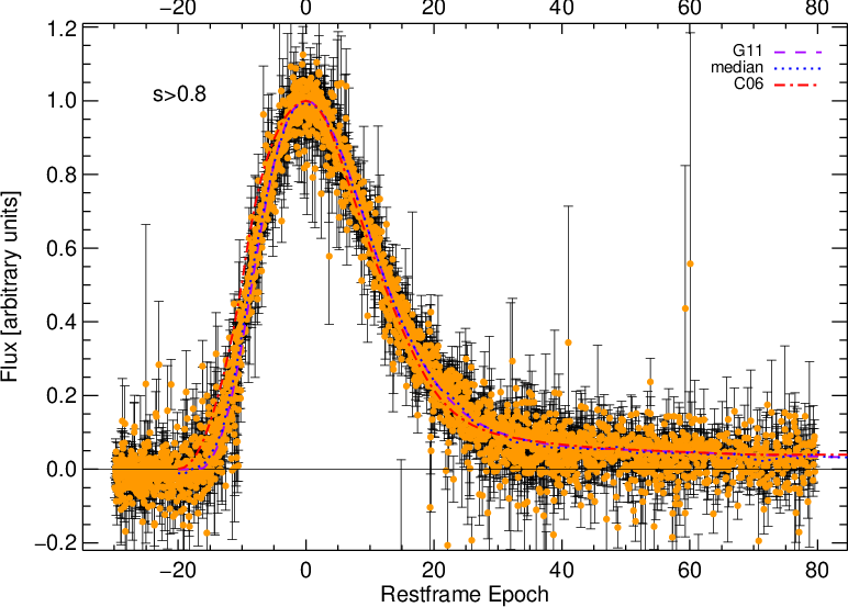
To make a combined rise-time study of all SNe Ia in each sample, we process each lightcurve as described in § II.1. We then take the restframe -fluxes of the low-stretch SNe Ia and overlay them on a single plot, as shown in Figure 1. For the rise-time region, we use early data, before a characteristic transition epoch days to fit it to the model of Equation 2 (see Figure 2). Minimizing the of the best fit model with respect to the data provides the best stretch-corrected rise-time. The choice of the transition epoch used affects the fit, as will be shown in § IV.5. We perform an iterative outlier rejection (similar to C06) to discard any data points that strongly deviate from the fit according to Chauvenet’s criterion [77]. For the total sample, this corresponds to and discards 25 (out of 449) data points, but does not affect the final fit.
The early time fit of the aggregate LC, nevertheless, does not take into account uncertainties in the SN fit parameters and the photometric redshift. Errors in the redshift estimate induce small changes in stretch (24). Additionally, the use of a common SED for the LC fit as well as for the -corrections introduces strong correlations, as do the uncertainties of maximum date and stretch of each SN fit. We handle these by shifting the photometric redshift according to its error (for those SNe Ia with photo-) in a Monte Carlo (MC) fashion. For each new redshift a corresponding fit provides the new LC parameters (stretch, date of maximum and flux scales) and their respective errors (and covariance matrix). These values and errors, in turn, are used to generate a new set of random LC values (for SNe with and without photo-) that determine the model SED for each epoch. The -corrections are recalculated for the new set of redshift and LC parameters. For each of these realizations we fit the rise-time data of all SNe to the model and get the best fiducial, stretch-corrected rise-time and slope , respectively. The final values are drawn from the median of all realizations combined. The statistical uncertainties in the parameters are given by the 1 uncertainties in the distribution (see Figure 3). The distribution is broader for low- because of the smaller sample size,and because the low- sample includes more SNe with photometric redshifts, and hence larger errors in (see G11 for details).
Final rise-times for the SNLS, SDSS-II and nearby samples are shown in Table 2. The different samples agree well with each other providing no evidence for evolution. This is confirmed by the fiducial rise-time of the SNLS SNe Ia at . Rise-times for different SNLS stretch populations after the primary LC-width, or stretch, correction are also consistent. However, the data are also in agreement at a level with a secondary slight trend for longer fiducial rise-times in fast decliners. High-stretch SNe () have the shortest stretch-corrected rise-times, shorter than mid-stretch SNe (), and low-stretch () also seem to follow this trend. In the next sections, we investigate systematic effects that could modify these results.

IV.2. Comparison of single- and two-stretch fits
Here, we investigate differences arising from the parameterization of the LC in two pieces (rising and falling) as in Equation 1, and as done in H10. We process our data by fitting it with a 2- model, and we find that the rise-stretch and fall-stretch are consistent within the errors, although the average rise-stretch is slightly larger than the fall-stretch: (RMS of 0.24). The mean rise-stretch is also larger than the stretch from the 1- model, (RMS of 0.17) (see Figure 4). This can be explained as the day of maximum gets pushed to later times by more than half a day, (RMS of 1.77).
The mean error in the peak date is much larger for the 2- fits, (RMS of 0.53) (see Figure 5). An incorrect estimate of the date of maximum has a direct effect on the rise-time calculation. For our MC technique, in which the fit parameters are varied according to their errors, large uncertainties in the peak epoch will affect the final rise-time even more. Our initial cut of days rejects more than 80% of the 2- fits of the SNLS sample (40% for the 1- fits), including all low- objects and all SNe Ia. We therefore relax the cut to days for the 2- fits.
We do not change our low- definition for the 2- fits to as this would reflect only the early part of the LC. If we were to use the fall-stretch instead, some low- candidates would have even lower stretch values. Instead we note that most candidates have a mean 2- stretch, i. e. , closer to the single-stretch: with 0.05 RMS, and use this to separate the different stretch samples. This definition keeps most of the low- candidates and is the best overall description of the lightcurve.
With the new stretch values we derived for the 2- fits, we repeat the procedure to estimate the fiducial rise-time, using the rise-stretch instead of the single stretch values for the -correction and normalization of all pre-maximum epochs. We obtain shorter stretch-corrected rise-times than the 1- approach, about 1-2% for the different SNLS samples (5% for SNe Ia at ), but still within the uncertainties. The decrease in fiducial rise-time with the 2- respect to the 1- fit comes partially from the compensation for the higher rise-stretches measured.
The 2- technique introduces new parameters in the fit, and we want to assess if an improvement is simply due to the increased complexity of the model, or if there is a real advantage in using it. To compare the two models, we use the Bayesian Information Criterion, , a tool that gives weight to the number of parameters of the fit, , as well as the total data used, [69]. By summing all the individual core LC fits ( days) of all SNe, we find that the 1- fit gives a smaller BICvalue: , compared to the 2- value: (the average per degree of freedom for the individual 2- fits is slightly better, , than for the 1- technique: ), i. e. the 2- technique did not lead to a better fit once the increase in parameters is taken into account. If we only consider the rise portion of the lightcurve (for which we use the same quadratic fit for both techniques), we obtain a lower chi-square per degree of freedom for the 1- approach, , than for the 2- fit: . The SNLS systematic uncertainties from different LC fits, 2- and a newer SiFTO version different from G11, are shown in Table 3.
Similar results are found for the SDSS and low- samples. The core LC fits are better for the 1- fits whereas the early rise-time fit is better for the 2- approach, according to the BIC criterion. The average rise-stretch is larger than the fall-stretch (by for the SDSS and for the low- sample) partly because of a mean shift in the peak date (of and days for the SDSS and low-, respectively). The mean errors in peak time are somewhat lower ( for the SDSS and for the nearby sample). The final rise-times obtained are comparable for both techniques, although the low- 2- result is lower than its 1- counterpart.
In the present study, we do not find a significant change in the rise-times of different samples for the two parameterizations considered: 1- and 2-, except for the nearby set for which a difference is found. Our 2- technique that is based on an adapted two-piece SiFTO fitter provides more uncertain peak date estimates. Requiring accurate maximum epochs affects the number of SNe we can use in the fit for the 2- technique (see section III). We find that using only SNe with days is good enough for the fit but the number of objects used is less than for the 1- technique, even though we use a tighter criterium for that fitter of days.
Although the statistical analysis of the fiducial rise-time remains unchanged with the parameterization used, Figure 4 shows that individual rise- and fall-stretches in the 2- technique do not vary equally for different SNe. The linear fits show that lower- SNe Ia tend to have larger rise-stretches and shorter fall-stretches for their respective 1- (a higher difference between the two) as compared to higher- SNe Ia. The slopes of rise- and fall-stretch are different by more than 3.
| Sample | (1-) | (1-) (days)* | (2-) | (2-) (days)* | |
|---|---|---|---|---|---|
| SNLS | 134 | 87 | |||
| 12 | 8 | ||||
| 55 | 31 | ||||
| 67 | 48 | ||||
| SNLS | 102 | 15 | |||
| Nearby | 16 | 15 | |||
| SDSS-II | 64 | 36 | |||
| 23 | 12 | ||||
| 41 | 24 | ||||
- *
Statistical MC errors only


| Systematic | Rise-time (days) | Difference (days) | ||||
| all | low- | mid- | high- | low- - mid | mid- - high- | |
| () | () | () | ||||
| STANDARD | ||||||
| LC-FIT | ||||||
| 1- new SiFTO | 17.14 | 18.46 | 17.99 | 16.57 | 0.47 | 1.42 |
| 2- | 16.92 | 17.89 | 17.56 | 16.62 | 0.97 | 0.94 |
| TEMPLATE | ||||||
| NEW (conley09f) | 16.94 | 18.33 | 17.70 | 16.59 | 0.63 | 1.11 |
| C06 (nugent05)* | 18.77 | 20.13 | 19.68 | 18.21 | 0.45 | 1.47 |
| SALT2 | 18.16 | 19.13 | 18.77 | 17.57 | 0.36 | 1.20 |
| TRANSITION EPOCH | ||||||
| d | 17.22 | 18.68 | 17.56 | 16.95 | 1.12 | 0.61 |
| PHOTOMETRY | ||||||
| Fr phot, | 17.21 | 17.96 | 17.40 | 16.96 | 1.02 | 0.44 |
| Ca phot, free | 17.18 | 18.07 | 17.50 | 16.86 | 1.03 | 0.64 |
| POWER LAW | ||||||
| 16.83 | 17.87 | 17.26 | 16.68 | 0.61 | 0.58 | |
- *
This template is based on an old limited SN sample and is not included in the final systematic error budget.
IV.3. Comparison of different templates
The template used in C06 descended from Nugent et al. [58] and the early portion was based on a limited number of SNe Ia. Using this template to calculate the rise-time, we obtain 19.33 days, in agreement with the result obtained in C06 of 19.10 days.


The fiducial stretch-corrected SN Ia rise-time is dependent on the SED template used (see Figure 6), in particular on the rather arbitrary definition of a SN. This is especially important when comparing rise-times from different sources, where various templates can lead to different rise-times. A SN is defined here as the mean stretch of the training sample for the template we use, which is the same as in G11. If we correct rise-time of the C06 template for the different definitions, by comparing the fits directly (see Figure 7), i. e. a SN for the G11 template corresponds to a for the C06 template, we then obtain 18.77 days. This averaged correction partially accounts for the early wide behavior of the C06 template (see Figure 2). The simple change of definition is not sufficient to fully compensate the effect of an incorrect early template, so that a longer stretch-corrected rise-time is still obtained. We get similar long rise-times with the C06 template applied to the 2- technique, indicating that this parameterization is not independent of the template used.
Newer templates trained with the well-sampled data of the SNLS, like the one used in G11, or a more recent version trained with a larger sample (used for SiFTO in Guy et al. 26), give consistent rise-times after correction for the different definition. Table 3 shows the rise-times for different templates.

IV.4. Comparison with SALT2
We investigate here the use of a different LC fitter, SALT2 [25]. This fitter also makes use of different templates from the ones presented in the previous section, so that we are actually probing two systematics simultaneously: template and LC fitter.
In order to do this, we fit all SNe Ia with SALT2 in the range days. A direct comparison of their SiFTO stretch and parameter from SALT2 is shown in Figure 8 through a linear fit. We calculate restframe, stretch-corrected epochs using the redshift and a corresponding stretch (for each X1 parameter): . Every data point matching restframe -band is -corrrected by taking the SED for each restframe epoch based on Eq. 1 of Guy et al. [25] with , and the color obtained from the SALT2 fit, and integrating it in the appropriate filter at the proper redshift. We then fit the aggregate LC points of the early rise ( days) to the quadratic rise model.

Similarly, we take into account errors with a MC that shifts the fit parameters ( if necessary, and , , and color) according to their covariance matrix, and re-calculate a stretch from this, as well as a new K-correction for each point of each simulation. The median of all iteriations, the final fiducial rise-time we obtain for the normal- population, is days. This is larger by days than the standard SiFTO 1- and 2- rise-times. Although the SALT2 template is different than the templates we use (see Figure 6), it is not as extreme as the C06 template. Clearly, the use of the LC fitter also affects the measured rise-time and is an important systematic. The differences between SN Ia populations are still consistent as shown in Table 3.
IV.5. Transition Epoch
The transition epoch is the minimum epoch used in the core LC fit and the maximum epoch allowed in the early rise-time fit. Its value can affect the quality of the fit but also the resulting rise-time (and even the quadratic behavior of the rise). A higher value, like days, increases the amount of data for the early-time fit, but the rise may no longer follow a simple quadratic relation. Figure 9 shows that rise-time fits with different transition times and a fixed power fit (quadratic ) for the SNLS do not change much up to a maximum value of days, where the rise-time starts to diverge. We use here the standard days used in other studies but add a systematic uncertainty to the rise-time based on the differences at days (see Table 3).

IV.6. Zero scale
Wrong photometric subtraction affects fluxes that are close to zero and strongly influences the final stretch-corrected rise-time calculation. To study this systematic error, we add a nuisance parameter, , to the quadratic form (Eq. 2) that will absorb any general photometric error. For a good photometry, we should obtain values close to zero. In our study, we get , an off-zero value reflecting the large dispersion of the fluxes near zero (median of with 0.03 RMS) but small enough to represent a negligible effect on the rise-time. Consistent rise-times are obtained with free/fixed values for the photometry processed via the French and Canadian reconstructions, as seen in Table 3.
The importance of this parameter can be observed in Figure 10, in which different values in the range , or a 5% maximum shift of the normalized flux at peak, result in rise-times shifted by several days. We emphasize therefore the importance of proper photometry, well-sampled to dates even before explosion, to correctly calculate and not affect the rise-time.
IV.7. Different rise power laws
Other parameters that could influence the fiducial rise-time behavior are and the rise power in Eq. 2. We find for the normal- SNLS population (arbitrary flux units) and an assumed quadratic form. If we relax the quadratic rise assumption and allow the power of the rise-time model to be free (free and fixed ), we obtain (stat). Rise-times fitted with this new power law are lower for all stretch populations but consistent with their quadratic equivalents.
Figure 10 shows the relation between the assumed power-law, , and the measured stretch-corrected rise-time, for the normal SN Ia sample. A higher makes the LC rise faster. In order to compensate for this, the duration of the rise to maximum of the fit becomes longer. This effect has a high degree of degeneracy and correlation between the two fit parameters, and . A very similar trend is observed for the different stretch samples. Furthermore, if the quadratic form is relaxed for all populations, we obtain increasing power laws and rise time for higher- SNe (Table 4). This variation shows again the clear difference in the rise-time region for the sub-samples of SNe Ia.
| Sample | (days)* | * |
|---|---|---|
| SNLS | ||
| High- | ||
| Mid- | ||
| Low- |
- *
Statistical MC errors
Although the systematic uncertainty from this variation is also highly correlated with the transition time, we still include it in the total systematic error budget.


V. Results and Discussion
The final fiducial rise-time, , for all SNe Ia in the SNLS calculated via the single-stretch method is (statistical)(systematic). The statistical uncertainty represents the 1 distribution of the MC simulations and the systematic uncertainty comes from the different effects considered in the previous section (added in quadrature) and shown in Table 3. This agrees with the value found via the two-stretch technique.
We find that the fiducial stretch-corrected rise-times are consistent for fast and slow decliners, independently of different fit characteristics such as the template or lightcurve fitter. Mid-stretch SNe Ia () have a fiducial rise-time (stat)(syst) days longer than their high-stretch counterpart (), barely a result. With even lower significance, low-stretch SNe Ia show a difference with respect to the high-stretch population of (stat)(syst) days.
Although we do not measure individual rise-times, an estimate based on the stretch of each object can be obtained from the fiducial rise-time. For the single-stretch case we do , where the subscript denotes each individual SN and is the fiducial rise-time. Individual rise-times for the low- population lie in the range of 10-14 days. For the normal- population, they lie in the range of 14-21 days.
V.1. Comparison to previous studies
As mentioned in § IV.3, the different definition of a fiducial lightcurve across different templates makes the comparison of stretch-corrected rise-times from several studies quite difficult.
Having that in mind, recent studies [74, 29], including the present one, agree that the average rise-time of SNe Ia is shorter than previously thought. With more data, better-sampled at early times, the new templates, as well as LC-fitting techniques, provide evidence for a 1-2 days shift in the average rise-time of SNe Ia with respect to previous studies [66, 12], although the precise value is heavily dependent on the definition of a fiducial LC template.
Although we use the same technique as C06, the template they used was trained with a handful of SNe Ia and consequently had a rise-time behavior to maximum quite different from the current templates. Their rise-time is longer than the one we find here, even after correcting for our definition.
We also analyze the nearby and SDSS-II datasets with our same template and LC fitter. H10 used a much larger SDSS-II sample (361 SNe) than used here (the 146 SDSS-II SNe from Holtzman et al. 35). Our SDSS-II fiducial rise-time agrees well with theirs. They argue that the two-stretch technique presents a much better parameterization than a single parameter approach. We do not agree with those findings for our aggregate rise-time fit approach, neither for the SNLS nor the SDSS and low- data. This could be due to the use of a different fiducial LC template and fitter that differ in the rise-time region from the ones they use (G11 and modified SiFTO vs MLCS2k2, Jha et al. 39), in particular the stretch they calculate is not based on multiple bands. The Bayesian Information Criterion for the core LC fits suggest that the inclusion of an additional parameter to model SN Ia lightcurves does not provide a valuable improvement of the fit. The quadratic fit of the early rise-time data is not strongly affected by the parameterization either. Individual rise-times, on the other hand, could benefit from such an independent parameterization, as shown in Figure 4.
Based on our calculations of the fiducial rise-time for different samples across the redshift range , we do not find evidence for a significant evolution in the early portion of SN Ia lightcurves. Dividing the SNLS sample into three populations according to their stretch values, we measure the average rise-times for each sub-group and find them to be consistent. Although at low confidence, the data also agree with a trend of faster fiducial rise-times for brighter and slowly declining SNe Ia after the primary stretch correction, for the SNLS and SDSS-II. H10 obtained a similar trend for the individual rise-times of SDSS-II objects.

V.2. 56Ni masses


In order to estimate the 56Ni masses, we need to calculate bolometric luminosities. We integrate the model SEDs for each SN across all observed bands. This omits the near-infrared (NIR), which accounts for a substantial fraction of the bolometric luminosity, so we must apply a correction factor. In Howell et al. [37] the IR percentage for normal SNe Ia is estimated via integration of proper SEDs corrected for each SN in the region outside the observed spectrum, under some assumptions. For low- SNe Ia, SEDs are not as fully sampled. We instead use a very broad approximation based on the IR fraction found for SN1999by and SN2004eo [33, 22, 76]: . The fraction is at least higher than for normal SNe Ia. We use a standard value (and for the normal-) to calculate via Equations 3 and 4 the 56Ni mass.
In order to account for the errors in the LC parameters, we carry out this computation for every realization of the LC data in the MC of § IV.1, and use the median of each SN to calculate the final 56Ni masses, as shown in Figures 11 and 12. We also include the error on the conversion factor , which can also slightly vary with 56Ni mass. The 56Ni masses lie between 0.05-0.35 for the low- and 0.1-0.8 for the normal- populations. Our estimates are lower than typical values in the literature because of the lower rise-times. They are similar for both parameterizations of the lightcurve (see Figure 13).
Figure 12 shows 56Ni masses as a function of the individual rise-times for all SN Ia. The relation of Ni mass and rise-time is expected from the use of Arnett’s rule. The individual rise-times are obtained from the fiducial rise-time and the individual stretches, so that 56Ni mass also relates with stretch. However, one can observe that, as rise-time is more independent of stretch for the 2- technique, there is a more diverse 56Ni mass range for each stretch population. It may be beneficial to divide the LC into separate regions, rise and fall, to disentangle the rise portion from the primary width-luminosity driver, when studying early-time effects of SNe Ia.

V.3. Secondary lightcurve parameters
The need for secondary parameters to describe SNe Ia at early times, beyond the traditional core LC parameter like stretch or , would have important consequences for the understanding of SNe Ia. To the precision achieved in this study, these secondary effects in the early rise-time region do not seem necessary to describe SN Ia LCs. We find a low-significance trend towards longer rise-times in fast decliners after stretch correction. If confirmed with more data, this would mean that rise-times do not correlate to second-order with stretch and 56Ni mass. This would suggest that beyond the radioactive decay of nickel which only sets in later in the LC, some other parameter in the initial explosion in the outer ejecta could play a role.
Besides a primary parameter responsible for the luminosity-width relation of SNe Ia, like 56Ni mass (from a varying density at the transition of subsonic deflagration to supersonic detonation in the delayed-detonation scenario), Höflich et al. [34] predict that there could be other variables like the C/O ratio of the WD progenitor that would affect the early part of the lightcurve. Higher C/O ratios result in a smaller binding energy at time of the explosion of the WD. In turn, this leads to higher expansion velocities meaning a faster photosphere recession and a shorter rise to maximum light. Lower main-sequence masses (during He-core and He-shell burning for example) can lead to higher C/O ratios. This would imply that lower-stretch SNe Ia with longer rise-times come from higher masses. The fact that low-stretch SNe Ia are primordially found in old environments suggest that their progenitors are long-lived and of low-mass [24], in contradiction to these findings.
On the other hand, low-stretch SNe having longer rise-times is reminiscent of the behavior predicted by Fink et al. [19] for the double-detonation of sub-Chandrasekhar models. The initial He-shell detonation on the WD surface can lead to a detonation of the CO core of the WD. Varying WD masses (0.8-1.4), and with it their central core and shell densities, give rise to a variety of 56Ni masses and burning products powering the lightcurve. Particularly they find that brighter events have faster rise-times. This is because brighter explosions produce more core 56Ni that expand faster with less opacity in the outer shells from iron-group-elements created in the He-shell detonation. Their effect is anti-corrected with stretch, which would indicate a primary correction rather than a secondary one. In this picture, the lightcurve and the rise-time are directly related to the initial mass of the WD. Lower-mass WDs (of ) have lower He-shell and CO core densities leading to a distribution of burning products that give rise to slower rise-times for low-stretch SNe Ia. Lower mass WDs producing fast decliners would agree with the aforementioned observations of older host environments.
Another interesting feature of the predictions by Fink et al. [19] is that the contribution of other radioactive elements like 52Fe and 48Cr of short decay times can make the rise-time longer. This is particularly true for subluminous SNe Ia, which in their models produce as much as 20% of these radioactive nuclei, particularly 44Ti, which does not contribute to the early lightcurve, but is known to be observed in the spectra as well. These yields are a direct consequence of the initial He-shell detonation.
VI. Conclusions
We have constructed aggregate restframe -band LCs of a sample of spectroscopic and photometrically identified SNe Ia at from the SNLS. We obtain fiducial rise-times that are consistent with measurements for the low- and SDSS-II samples calculated here with the same techniques. We extend our SNLS sample and show that there is no significant evolution in the early portion of SN Ia lightcurves up to .
We find that the use of a two-stretch parameterization for the lightcurve fits of SNe Ia is equivalent to the single-stretch parameterization for the rise-time study of aggregate lightcurves. We confirm the consistency for the SDSS-II and SNLS samples while the nearby set has a rise-time lower for the 2- technique and discrepant with all other calculated rise-times. We insist in the importance of proper lightcurve fitters with parameters that can take into account earlier parts of the lightcurve (stretch vs ) and that include multi-band information, and of templates trained with sufficient SNe with early time data. We also find indications that the 2- approach might be useful for detailed studies of individual rise-times, as in Hayden et al. [29], Ganeshalingam et al. [21].
We have compared the early region fits for different stretch population of the SNLS. We find that the stretch-corrected rise-times are consistent within uncertainties for slow and fast decliners. We extend this result to the lowest stretch objects. These findings are independent of systematics such as the maximum epoch allowed in the early time fits, as well as on the two LC parameterizations assumed. The present study averages over samples which can have obvious difficulties like the low statistics of the low-stretch population. At a low significance of , our results also agree with a trend for longer rise-times in fast declining SNe Ia. If these indications are confirmed, then SN Ia explosions differ beyond a single parameter orchestrating the lightcurve of SNe Ia. Secondary parameters in the early rise region would be necessary to fully model the lightcurves and could provide useful insights into SN Ia explosions. Such an indication is also found for the SDSS-II, as in H10.
However, to the precision attained in this study, SNe Ia remain extremely homogeneous all the way to very early times. One single lightcurve parameter, that possibly translates to a unique physical variable, like the transition density of deflagration to detonation in the delayed detonation model, can account not only for the core lightcurves of SNe Ia, but largely for the rise-time as well. The similarity of SN Ia lightcurves (after stretch-correcting) argue for a real common origin, with subluminous SNe Ia at the extreme end of the population.
The fiducial rise-time we find translates into 56Ni masses of for all SNe Ia (and for low- SNe Ia). Although our assumed IR contribution to the bolometric luminosity is uncertain, extremely low amounts of radioactive 56Ni seem enough to power a faint SN Ia, less than that the amount found by Filippenko et al. [18], Leibundgut et al. [49]. Our SNe with the lowest radioactive nickel yield even rival with peculiar extreme objects such as the ones found by McClelland et al. [55], Kasliwal et al. [43], Poznanski et al. [65], and pose a challenge to explosion models.
Such weak explosions seem unlikely to be the outcome of a runaway of a WD near the Chandrasekhar mass. Sub-Chandrasekhar models have been indeed a natural way of explaining subluminous SNe Ia [52, 85, e. g.], and possibly all SNe Ia [19, 71, 83]. Located in passive environments that are characteristic of old populations, low-mass WDs seem a promising progenitor of subluminous SNe Ia. With recent rejections of a high fraction of red giant donors [29, 6], a double degenerate merger leading to the sub-Chandrasekhar explosion of a low-mass WD with very low 56Ni yield appears increasingly plausible. If SNe Ia share a common explosion and progenitor mechanism, a varying progenitor WD mass could possibly explain the different SN Ia radioactive yield and luminosity, and their environment. More and better simulations need to test the validity of this picture. Pakmor et al. [59], for example, modelled the merger of two WDs and obtained a subluminous SN Ia explosion with of synthetized 56Ni, in agreement with the bulk of our low- objects but in disagreement with the expected progenitor masses from the environments. More theoretical development need to complement the abundant current and coming observations of SNe Ia.
We thank Brian Schmidt for valuable comments. We are grateful to the CFHT Queued Service Observations Team and the entire SNLS collaboration. We acknowledge the support from our funding agencies: NSERC, CIAR, CNRS and CEA. MS acknowledges support from the Royal Society.
References
- [1] Aldering, G., Knop, R., & Nugent, P. 2000, AJ, 119, 2110
- [2] Altavilla, G. et al. 2004, MNRAS, 349, 1344
- [3] Anupama, G. C., Sahu, D. K., & Jose, J. 2005, A&A, 429, 667
- [4] Arnett, W. D. 1982, ApJ, 253, 785
- [5] Arnett, W. D., Branch, D., & Wheeler, J. C. 1985, Nature, 314, 337
- [6] Bianco, F. B. et al. 2011, ArXiv e-prints
- [7] Boulade, O. et al. 2003, in Society of Photo-Optical Instrumentation Engineers (SPIE) Conference Series, Vol. 4841, Society of Photo-Optical Instrumentation Engineers (SPIE) Conference Series, ed. M. Iye & A. F. M. Moorwood, 72–81
- [8] Branch, D. 1992, ApJ, 392, 35
- [9] Bravo, E. & García-Senz, D. 2008, A&A, 478, 843
- [10] Bravo, E. et al. 2010, ArXiv e-prints
- [11] Colgate, S. A. & McKee, C. 1969, ApJ, 157, 623
- [12] Conley, A. et al. 2006, AJ, 132, 1707
- [13] —. 2008, ApJ, 681, 482
- [14] —. 2011, ApJS, 192, 1
- [15] Contardo, G., Leibundgut, B., & Vacca, W. D. 2000, A&A, 359, 876
- [16] Domínguez, I., Höflich, P., & Straniero, O. 2001, ApJ, 557, 279
- [17] Filippenko, A. V. 1997, ARA&A, 35, 309
- [18] Filippenko, A. V. et al. 1992, AJ, 104, 1543
- [19] Fink, M. et al. 2010, ArXiv e-prints
- [20] Gallagher, J. S. et al. 2008, ApJ, 685, 752
- [21] Ganeshalingam, M., Li, W., & Filippenko, A. V. 2011, MNRAS, 1265
- [22] Garnavich, P. M. et al. 2004, ApJ, 613, 1120
- [23] Goldhaber, G. et al. 2001, ApJ, 558, 359
- [24] González-Gaitán, S. et al. 2011, ApJ, 727, 107
- [25] Guy, J. et al. 2007, A&A, 466, 11
- [26] —. 2010, A&A, 523, A7+
- [27] Hamuy, M., Phillips, M. M., Suntzeff, N. B., Schommer, R. A., Maza, J., & Aviles, R. 1996, AJ, 112, 2391
- [28] Hayden, B. T. et al. 2010a, ArXiv e-prints
- [29] —. 2010b, ArXiv:1001.3428
- [30] Hicken, M. et al. 2007, ApJ, 669, L17
- [31] —. 2009, ApJ, 700, 331
- [32] Hoeflich, P., Mueller, E., & Khokhlov, A. 1993, A&A, 268, 570
- [33] Höflich, P. et al. 2002, ApJ, 568, 791
- [34] —. 2010, ApJ, 710, 444
- [35] Holtzman, J. A. et al. 2008, AJ, 136, 2306
- [36] Howell, D. A. 2001, ApJ, 554, L193
- [37] Howell, D. A. et al. 2009, ApJ, 691, 661
- [38] Hsiao, E. Y., Conley, A., Howell, D. A., Sullivan, M., Pritchet, C. J., Carlberg, R. G., Nugent, P. E., & Phillips, M. M. 2007, ApJ, 663, 1187
- [39] Jha, S., Riess, A. G., & Kirshner, R. P. 2007, ApJ, 659, 122
- [40] Jha, S. et al. 2006, AJ, 131, 527
- [41] Kasen, D. 2010, ApJ, 708, 1025
- [42] Kasen, D., Röpke, F. K., & Woosley, S. E. 2009, Nature, 460, 869
- [43] Kasliwal, M. M. et al. 2010, ApJ, 723, L98
- [44] Kelly, P. L. et al. 2010, ApJ, 715, 743
- [45] Khokhlov, A., Mueller, E., & Hoeflich, P. 1993, A&A, 270, 223
- [46] Khokhlov, A. M. 1991, A&A, 245, 114
- [47] Krisciunas, K. et al. 2003, AJ, 125, 166
- [48] —. 2004, AJ, 127, 1664
- [49] Leibundgut, B. et al. 1993, AJ, 105, 301
- [50] Leonard, D. C., Li, W., Filippenko, A. V., Foley, R. J., & Chornock, R. 2005, ApJ, 632, 450
- [51] Lira, P. et al. 1998, AJ, 115, 234
- [52] Livne, E. 1990, ApJ, 354, L53
- [53] Maeda, K. et al. 2010, ApJ, 712, 624
- [54] Mazzali, P. A., Röpke, F. K., Benetti, S., & Hillebrandt, W. 2007, Science, 315, 825
- [55] McClelland, C. M. et al. 2010, ApJ, 720, 704
- [56] Neill, J. D. et al. 2011, ApJ, 727, 15
- [57] Nugent, P., Branch, D., Baron, E., Fisher, A., Vaughan, T., & Hauschildt, P. H. 1995, Physical Review Letters, 75, 394
- [58] Nugent, P., Kim, A., & Perlmutter, S. 2002, PASP, 114, 803
- [59] Pakmor, R., Kromer, M., Röpke, F. K., Sim, S. A., Ruiter, A. J., & Hillebrandt, W. 2010, Nature, 463, 61
- [60] Pastorello, A. et al. 2007, MNRAS, 376, 1301
- [61] Perrett, K. et al. 2011, in preparation
- [62] Phillips, M. M. 1993, ApJ, 413, L105
- [63] Phillips, M. M., Lira, P., Suntzeff, N. B., Schommer, R. A., Hamuy, M., & Maza, J. . 1999, AJ, 118, 1766
- [64] Phillips, M. M. et al. 1992, AJ, 103, 1632
- [65] Poznanski, D. et al. 2010, Science, 327, 58
- [66] Riess, A. G. et al. 1999, AJ, 118, 2675
- [67] —. 2005, ApJ, 627, 579
- [68] Roepke, F. K. et al. 2010, ArXiv e-prints
- [69] Schwarz, G. E. 1978, Annals of Statistics, 6, 461
- [70] Shigeyama, T. et al. 1992, ApJ, 386, L13
- [71] Sim, S. A., Röpke, F. K., Hillebrandt, W., Kromer, M., Pakmor, R., Fink, M., Ruiter, A. J., & Seitenzahl, I. R. 2010, ApJ, 714, L52
- [72] Smith, J. A. et al. 2002, AJ, 123, 2121
- [73] Stanishev, V. et al. 2007, A&A, 469, 45
- [74] Strovink, M. 2007, ApJ, 671, 1084
- [75] Sullivan, M. et al. 2010, MNRAS, 406, 782
- [76] Taubenberger, S. et al. 2008, MNRAS, 385, 75
- [77] Taylor, J. 1997, Introduction to Error Analysis, the Study of Uncertainties in Physical Measurements, 2nd Edition, ed. Taylor, J. (University Science Books)
- [78] Timmes, F. X., Brown, E. F., & Truran, J. W. 2003, ApJ, 590, L83
- [79] Truran, J. W., Arnett, W. D., & Cameron, A. G. W. 1967, Canadian Journal of Physics, 45, 2315
- [80] Tsvetkov, D. Y. 2006a, Peremennye Zvezdy, 26, 3
- [81] —. 2006b, Peremennye Zvezdy, 26, 4
- [82] Valentini, G. et al. 2003, ApJ, 595, 779
- [83] van Kerkwijk, M. H., Chang, P., & Justham, S. 2010, ApJ, 722, L157
- [84] Wang, X. et al. 2009, ApJ, 697, 380
- [85] Woosley, S. E. & Weaver, T. A. 1994, ApJ, 423, 371
- [86] Yamaoka, H. et al. 1992, ApJ, 393, L55