Heavy Quark Momentum Diffusion Coefficient from Lattice QCD
Abstract
The momentum diffusion coefficient for heavy quarks is studied in a deconfined gluon plasma in the static approximation by investigating a correlation function of the color electric field using Monte Carlo techniques. The diffusion coefficient is extracted from the long distance behavior of such a correlator. For temperatures , our nonperturbative estimate of the diffusion coefficient is found to be very different from the leading order perturbation theory, and is in the right ballpark to explain the heavy quark flow seen by PHENIX at RHIC.
pacs
12.38.Mh,11.15.Ha,25.75.-qI Introduction
The charm and the bottom quarks are very important tools in our quest to understand the nature of the quark-gluon plasma created in the relativistic heavy ion collision experiments. Since the masses of both of them are much larger than the temperatures attained in RHIC, and in LHC, one expects these quarks to be produced largely in the early pre-equilibrated state of the collision, and thus provide a window to look into the early stages of the fireball. Furthermore, perturbative arguments suggest that the energy loss mechanism for energetic heavy quarks in medium should be different from that of the light quarks. A comparative study of the energy loss for the heavy and light quark jets therefore leads to crucial insights into the way the quark-gluon plasma interacts.
For light quark jets, gluon radiation (“bremsstrahlung”) is expected to be the leading mechanism for energy loss in medium [1]. It has been argued that gluon bremsstrahlung is suppressed for jets of heavy quarks [2], and collisional energy loss may be the dominant mechanism for thermalization of not-too-energetic heavy quark jets [3, 4]. Since collision with a thermal quark does not change the energy of a heavy quark substantially, one would expect that the thermalization time of the heavy quarks is much larger than that of the light quarks. As most of the elliptic flow is developed early, the azimuthal anisotropy parameter, , of the hadrons with heavy quarks can be expected to be much less than that of the light hadrons.
Interesting predictions follow from these simple, weak coupling-based intuitions, which can be, and have been, checked in the RHIC experiments. One expects a mass ordering of the elliptic flow: . Here refer to the light hadrons, mesons of the family (one charm and one light quark) and those in the family (one bottom and one light quark). The nuclear suppression factor, , is also expected to show a hierarchy: . Experimentally, on the other hand, it was found that the heavy flavor mesons show a large elliptic flow, and a strong nuclear suppression, , the nuclear suppression being comparable to that of for GeV [5, 6].
Even if the kinetic energy of the heavy quark is , where is the temperature of the fireball, its momentum will be much larger than the temperature. It is, therefore, changed very little in a single collision, and successive collisions can be treated as uncorrelated. Based on this picture, a Langevin description of the motion of the heavy quark in the medium has been proposed [7, 3, 4]. , the elliptic flow parameter, can then be calculated in terms of the diffusion coefficient of the heavy quark in the medium. The diffusion coefficient has been calculated in perturbation theory [7, 3]. While the experimental results for the elliptic flow of the charmed mesons and its dependence seem to be well described by this formalism for moderate GeV, the value of the diffusion coefficient needed to explain the experimental data is found to be at least an order of magnitude lower than the leading order (LO) perturbation theory (PT) result [6] 11 1 Note that the observed flow depends not only on the diffusion coefficient but also on various other details like the geometry of the collision, evolution, equation of state of the plasma, etc. See [8] for a comprehensive review. Furthermore, the LOPT value itself leads to heavy flavor flow which falls way short of the data. The contribution of the next-to-leading order (NLO) in perturbation theory has been calculated recently [9]. Although, it was found to change the LO result by a large factor at temperatures , this should perhaps be taken as an indication of the inadequacy of perturbation theory in obtaining a reliable estimate for the diffusion coefficient in the temperature range of interest.
A nonperturbative estimate of the diffusion coefficient, , in QCD is, therefore, essential to understand the heavy quark flow in the Langevin formalism. Lattice QCD, together with numerical Monte Carlo techniques, provides the only way of doing first principle nonperturbative calculations in the quark-gluon plasma. Unfortunately, such calculations are done in Euclidean space, and extracting a real time object like the diffusion coefficient requires an analytic continuation, which is extremely difficult. However, estimation of various transport coefficients have already been attempted, with varying degrees of success [10]. In order to estimate the heavy quark diffusion coefficient, one can study the correlator of the heavy quark current, . Early attempts to extract this way showed that the correlator has very little sensitivity to [11]. Preliminary results of a calculation of extracted from correlator, using much finer lattices than used before, have been presented recently in the temperature range between 1.5 — 3 for a gluon plasma [12]. They do find a value which is much lower than the LOPT result, and in the right ballpark to explain the experimental heavy quark flow.
Two of the difficulties in extracting the diffusion coefficient from correlator are: i) the behavior of the structure of the spectral function near the regime can affect the structure at low , and ii) the diffusion coefficient is obtained from the width of the narrow transport peak at , which is difficult to extract. In the infinitely heavy quark limit, another approach to the diffusion coefficient has been suggested in Refs. [13, 14]. In this static limit, the propagation of heavy quarks is replaced by Wilson lines, and the formalism of Ref. [3] reduces to the evaluation of retarded correlator of electric fields connected by Wilson lines [13]. In Ref. [13], this formalism was used to calculate the diffusion coefficient for the = 4, SU() gauge theory, using the AdS/CFT correspondence. A parametric dependence on coupling very different from weak coupling perturbation theory was obtained. On the other hand, for the pure SU(3) gauge theory, a leading order perturbative calculation of this correlator led to a negative value for the diffusion coefficient at moderate temperatures [15].
The formalism outlined in Ref. [14] is suitable for Monte Carlo calculation on the lattice. As we outline in the next section, this involves the calculation of Matsubara correlators of color electric field operators, and extracting the low frequency part of the spectral function from it. Of course, the usual problems of extraction of the spectral function from the Matsubara correlator mean that calculation of the diffusion coefficient remains a highly nontrivial task. A first attempt to calculate the diffusion coefficient from the electric field correlator lead to very large values of the diffusion coefficient, close to the perturbation theory value [16]. Preliminary results from a recent calculation [17], on the other hand, gave values in the temperature range 1.5-3 close to the experimental results.
In this work, we use the formalism of [13, 14] to calculate the diffusion coefficient of the deconfined gluonic plasma in a moderate temperature range, . The aim is to understand whether a small diffusion coefficient, as found in the analysis of the experimental data [6], is consistent with QCD. The plan of the paper is as follows. In the next section we outline the formalism. In Sec. III we explain the operators and the algorithm. Sec. IV has our results. A discussion of the results, including their connection with experiments, is contained in Sec. V. Some details of Secs. III and IV are relegated to the appendices.
II Formalism
In this section, we outline the formalism of Refs. [13, 14] in more detail. We first sketch the arguments leading to the Langevin formalism, and then discuss the quantum field theoretic calculation of suitable correlation functions. This discussion closely follows Refs. [3, 13, 14]. Then we discuss the issues related to the extraction of the diffusion coefficient from the Matsubara correlator.
It is easy to see why the motion of a quark much heavier than the
system temperature can be described in the Langevin formalism. If the
kinetic energy is , then the momentum, , is
not changed substantially in individual collisions with thermal gluons
and quarks, which can only lead to a momentum transfer . Therefore, the motion of the heavy quark is similar to a Brownian
motion, and the force on it can be written as the sum of a drag term
and a “white noise” , corresponding to uncorrelated random
collisions:
| (1) |
From Eq. (1) the momentum diffusion coefficient,
, can be obtained from the correlation of the force term:
| (2) |
The drag coefficient, , can be connected to the diffusion
coefficient using standard fluctuation-dissipation relations
[18]:
| (3) |
Here is the heavy quark mass.
To have a field theoretic generalization of Eq. (2), one
first introduces the conserved current for the heavy quark number
density, , where is the heavy quark field
operator. The force acting
on the heavy quark is given by and so, Eq. (2)
generalizes to
| (4) |
where is the spatial integral of the density correlator:
| (5) |
and is directly proportional to the number density for a system of non-relativistic quarks.
Since we are working in the heavy quark limit, the force term and the
number density term are easy
to infer:
| (6) |
where and are the two-component heavy quark and antiquark field operators, respectively, and is the color electric field. In leading order expansion in , only the electric field contributes to the force term.
With the substitution of Eq. (6), the real time correlator
in Eq. (4) can be calculated as the analytical continuation
of the Matsubara correlator,
| (7) |
The spectral function, , for the force term is connected
to by the integral equation [18]
| (8) |
The momentum diffusion coefficient, Eq. (4), is then
given by
| (9) |
Since we are working in the limit of infinitely heavy quarks, the
expression (7) simplifies considerably. The heavy quark
correlators give a static color field, besides an exponential
suppression factor coming from the heavy quark mass: , where
is the timelike gauge connection, and the delta function
comes because the infinitely heavy quark does not move spatially.
The exponential factor cancels with a similar factor from ,
resulting in a rather simple expression for the infinitely heavy quarks:
| (10) |
where is the Polyakov loop. Once again, intuitively it is easy to understand Eq. (10): for the infinitely heavy quarks, all that the force-force correlator gives is the correlator of color electric fields, connected through Wilson lines, and normalized by the Polyakov loop.
In order to connect measured on the lattice to
physical correlator of electric fields, we need to multiply by a
renormalization factor:
| (11) |
where is the lattice spacing dependent renormalization factor for the electric field correlator. A nonperturbative evaluation of the electric field operator used here is not available. However, the renormalization factor is expected to be dominated by the self energy correction, which can be taken into account by a tadpole correction [19]. In fact, with other discretizations of the electric field operator it has been found that the tadpole factor gives a very close approximation to the nonperturbative renormalization factor [20]. Here we use the tadpole factor to renormalize the electric field.
The extraction of from using Eq. (8) is an extremely difficult problem. In general, the kernel in Eq. 8 will have zero modes on a discrete lattice, making the inversion problem ill-defined. In the ideal case, one may be able to impose some reasonably general conditions on and be able to make the problem invertible. However, in situations like ours, where is measured only on data points with errors, the problem of extraction of becomes a completely ill-posed problem without any further input.
For some problems, a Bayesian analysis, with prior information in the form of perturbative results, has been useful. In general, though, a stable application of these techniques require both a very large number of points in the direction and very accurate data for . For the kind of extended objects we are considering, wrapping the lattice in the Euclidean time direction, it is very difficult to obtain both together, as the error on the correlators grows with the number of points in the direction.
Parameterizing in terms of a small number of parameters, therefore, seems to be a simple way to make the inversion problem well-posed. In our case, the leading order perturbative form of the spectral function . Also in the regime, we need to get a physical value of the diffusion constant using Eq. (9). The calculation of Ref. [13] got for the supersymmetric Yang-Mills theory. Motivated by this, we use a simple ansatz for the spectral function,
| (12) |
We do not include any running in , which is proportional to in the leading order. This approach is similar in spirit to that used in Ref. [21] to calculate electrical conductivity. Note that the NLO PT calculation of Eq. (10) leads to a negative value of , and in general, seems to deviate more from the lattice correlators than the LO result. So we use the LO form for the high part.
On the other hand, in the calculation with classical lattice gauge
theory [22], the spectral function of the color electric field
was found to have the behavior
So to crosscheck the dependence on our assumption, we also use a second fit form,
| (13) |
In practice, we use these postulated forms for to evaluate , and fit it to the long distance correlation function measured on the lattice. At large , of course, this form is not valid, and a complicated form, that takes into account the effect of the lattice Brillouin zones, will have to be considered. We tried using the free lattice spectral function instead of the term in Eqn. (12). However, that did not improve the fit quality and in particular, did not seem to capture the very short distance behavior of the data any better. So in this work, we restrict ourselves to the large distance regime in our fits, and expect that in this regime our simple form will suffice for a first estimate of the diffusion coefficient.
III Numerical Details
For the lattice evaluation of the correlator , we first need to
choose a discretization of the electric field. Following Ref. [14]
we choose the discretization
which is a direct latticization of the relation . As Ref. [14] suggests, this form of the discretization of the electric field is expected to be less ultraviolet sensitive than the more common discretization in terms of the plaquette variable.
The numerator of Eq. (10) can then be written as
| (14) |

The evaluation of , Eq. (14), is known to be difficult for large , because the signal-to-noise ratio decays exponentially. The multilevel algorithm [23] was indeed devised to take care of such problems. We adapted it for calculation of the electric field correlation functions. The lattice is divided into several sublattices. The expectation value of the correlation functions are first calculated in each sublattice by averaging over a large number of sweeps in that sublattice while keeping the boundary fixed. A single measurement is obtained by multiplying the intermediate expectation values appropriately. The number of sublattices and the number of sublattice averagings were tuned for the various sets, so as to get correlators with % level accuracy. An explicit example is shown in Fig 1 which illustrates the calculation of on a lattice with four sub-lattices, each with a thickness of three lattice spacings. It is important to note that one needs to store all the intermediate sub-lattice averages separately before they can be multiplied at end of the update of the whole lattice to construct the correlation functions. This imposes memory constraints for simulating large lattices.
The advantage of the multilevel algorithm can be seen from the following estimate: for , and , the correlator for , has the value of 1.317(2) from 350 multilevel measurements. The multilevel algorithm takes about 800 minutes to yield a single measurement on an Intel Xeon CPU processor with a speed of 2.5 GHz. For the same correlator, the standard method, using an updating with a combination of overrelaxation and heatbath steps, led to a value 1.2(2) for a runtime of about 8500 minutes on the same machine. Using the usual dependence of the error on runtime, the multilevel algorithm is seen to be about 300 times more efficient than the standard algorithm for for this lattice. The efficiency of the multilevel algorithm increases significantly for larger values of . A similar comparison for gives a factor of about 2000 (order of magnitude larger) relative efficiency for the multilevel algorithm. Thus, use of the multilevel scheme is indispensable for calculations at the larger values of 22 2 The efficiency is, of course, dependent on both and ., since these are required to be known with high precision for the extraction of the diffusion coefficient.
To get the results for various temperatures and volumes, we ran our simulations at a number of bare couplings with = 12 - 24 and = 2 - 4, for temperatures from just above to 3 . A reliable extraction of the diffusion coefficient was possible, however, only for lattices with . A list of such lattices used by us is given in Table 1 below. To obtain the temperature scale, we follow the strategy outlined in [24]. We calculate at each from the plaquette value. This is translated to a temperature scale at using the information of [25] and two-loop scaling formula with a fitted correction [26]. Temperatures for other are easily calculated from the temperature scale. The complete list of the lattice sizes, , and the corresponding temperature are shown in Table 2 in the appendix, which also shows the parameters used in the multilevel algorithm for each .
| 6.76 | 6.80 | 6.90 | 7.192 | 7.255 | |
| 20 | 20 | 20 | 24 | 20 | |
| 1.04 | 1.09 | 1.24 | 1.5 | 1.96 |
IV Results
In order to calculate , we calculated the electric field correlators, Eq.(10), for all the sets in table 2. From the correlators , can be calculated using Eq. (9). Use of the multilevel algorithm allowed us to get correlators at a few per cent level accuracy. In fact, we got % accuracy in all correlators except the two most central points of the set. Fig. 2 shows for this data set.
In order to get the momentum diffusion coefficient, , we use the ansatz Eq. (12) for , and fit the Euclidean correlator using Eq. (8). It was not feasible to do a three parameter fit: the parameters and are strongly correlated. For a large range of we can get very similar fit qualities. Instead, we fix and get an estimate of by doing a two-parameter fit. We discuss this further below and in Appendix B.


For the fit, minimization was carried out with the full covariance matrix included in the definition of . We typically obtained acceptable fits to the correlators for in the range , with . At shorter distances, lattice artifacts start contributing and the simple form of Eq. (12) does not work well. Also using the leading order lattice correlator instead of the continuum form did not improve the quality of the fit. We, therefore, restrict ourselves to the long distance part of the correlator.
In order to get a feel for the relative contributions of the different parts of the spectral function to the correlator, in Fig. 2 we show the correlators constructed from different parts of separately. We take the best fit form of Eq. (12) to the data set, for . The contributions to the total correlation function from the part of and that from the diffusive part, the first term in Eq. (12), are calculated separately using Eq. (8). In Fig. 2 we have called these parts LOC and DIFF, respectively, and the correlator reconstructed from the fitted spectral function has been called Fit. The correlator is seen to be dominated by the contribution from the term over the whole range of distance. However, the diffusion term has a substantial contribution near the center of the lattice. In Fig. 2 it contributes nearly 20 % at = 0.5. This is seen more clearly in the right hand panel of Fig. 2, where the total correlator, the best fit, and the diffusive part are shown normalized by the leading order correlator. Since the relative contribution of the diffusive part falls rapidly at shorter distances, it is difficult to get reliable estimates of , with the usual assorted tests like stability with small change in fit range, for our smaller lattices with = 12 and 16. So in what follows, we quote fit results for only for our finer lattices, with 20 and 24 (Table 1).
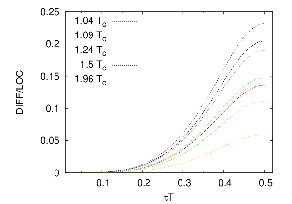

For these lattices, we obtained stable fits for the central part of the correlator, with in all cases. We did a fully correlated fit by including the inverse of the full covariance matrix in the function to be minimized, whenever such a function was well-behaved. That turned out to be the case in all sets except the one at the highest temperature, the set in Table 1. In this case we used an uncorrelated fit for our best estimate. The difference between the correlated and the uncorrelated fit was included in the systematic error. Our results for at various temperatures, using the ansatz Eq. (12) and , are shown in Fig. 4. The statistical error, shown by the solid (red) band, is obtained from a jackknife analysis.

The choice of for the central value was based on the fact that in all the sets, with , the diffusion term contribution to the spectral function, in Eq. (12), is numerically close to the large term, , when the diffusion term sets in (i.e., at ). Admittedly, this choice is somewhat arbitrary. In fact, the main source of uncertainty in our fit estimate, shown by the dashed (green) band in Fig. 4, is . To estimate the possible error introduced through our central value of , we varied in the range . We also looked at the fit form Eq. (13), and did the same exercise with it. The details of the fit results for Eqs. (12,13) and various are given in Appendix B. Quite often the fit value for these variations comes outside the statistical error band of Fig. 4. A systematic uncertainty band is therefore introduced, of sufficient size so as to include the central fit values for all these variations.
For the correlation functions of gluonic observables, major finite volume effects have been observed if the spatial size of the lattice is so small that some of the spatial directions get deconfined; on the other hand, at least for spatial correlation functions, finite size effects are small when the transverse directions are not deconfined [29]. To avoid large finite size effects, we choose lattices such that the spatial directions are confined. Since the electric field correlator also has contribution from the low part, it could be more sensitive to finite volume effects. However, as we discuss in appendix B, the correlation functions do not show any significant finite volume effect even when 2. Therefore we do not expect large finite size corrections to our results obtained from lattices with .
It is instructive to look at the relative contribution of the diffusive part to the total correlator at different distances. In the left panel of Fig. 3 we show the correlator coming from the diffusive part of the fitted spectral function, normalized by the leading order part, for all the lattices of Table 1. The notation is similar to that used in Fig. 2, except here we show the 1 band and not the best fit value. At all temperatures, except the one at the highest temperature, the diffusive part is seen to reach about 5 % level by . Note that the accuracy of our correlator is better than this. Also no significant trend of temperature dependence is seen in this figure. This is, of course, translated to the lack of significant temperature dependence of in this temperature regime, Fig. 4.
, the coefficient of the term in , is also of some interest.
In perturbation theory, the leading order spectral function is
| (15) |
To get an idea of the strength of the coupling at these temperatures, we use Eq. (15) and the fit coefficient , Eq. (12), for a nonperturbative estimate of . The estimate of obtained this way is shown in Fig. 3. If is the properly normalized current, then the NLO calculation of Ref. [15] can be used to connect this to . It is interesting to note that the coupling is rather small, about 1/4 near and going down to at 2 . This is in rough agreement with a similar measurement in Ref. [21] from fit to vector current correlators, and other, more detailed, calculations of at such temperatures from static observables [27].
In order to present our calculation in the context of RHIC, it seems convenient to use the Einstein relation between the diffusion coefficient, , and ,
| (16) |
In Eq.(16) is the drag constant. In Fig. 5 we show the diffusion coefficient in the temperature range , obtained using Eq. (16). The solid (red) error bar is the statistical error from a jackknife analysis. The bigger errorbars show the range of values covered by the different systematics analyzed in Table 3.

Two points are worth noting in this figure. First, the nonperturbative value of the diffusion coefficient is rather small in the temperature range considered. In the next section we discuss in more detail the comparison with perturbation theory, but the diffusion coefficient shown here is nearly an order of magnitude smaller than the leading order perturbation theory. Second, there is no strong temperature dependence, at least in the temperature range .
V Discussion
In this work, we studied the momentum diffusion coefficient, , of heavy quarks in a gluonic plasma. As mentioned in the introduction, the large elliptic flow of the heavy flavor mesons, seen in the PHENIX experiment at RHIC, seems to be well explained in a Langevin framework, if is large. Perturbation theory seems to be unstable for this quantity in the temperature regime of interest for RHIC physics, and the leading order PT prediction is at least an order of magnitude too small to explain the experimental data. Our aim in this work was to calculate the momentum diffusion coefficient nonperturbatively, and to see if the deviation from perturbation theory is of the size required to explain the experimental data.
Using the formalism of Refs. [13, 14], we calculated from
the correlator of , the electric field operator. From the
Matsubara correlator of the electric field, was calculated
through Eq. (9) using the ansatz for , Eq. (12).
In order to compare our results with the
perturbative calculation of [3] and experiments [6], we
used Eq. (16) to get the diffusion constant, . The
diffusion coefficient so obtained is found to be considerably
smaller than the LO PT estimate [3]. For high temperatures
such that , the leading order estimate of DT is
[3]
| (17) |
where is the color Casimir and is the number of flavors of thermal quarks. At very high temperatures, diverges as . As one comes down in temperature, Eq. (17) is not reliable any more and one needs to use the complete leading order estimate. To get this, we use Eq. (11) of [3], with determined using the plaquette measurement 33 3 The non-perturbative value of at the inverse lattice spacing scale, is obtained from the plaquette values [19], and then the 2-loop beta function is used to flow to the scale . and taken from lattice measurements [27]. For example, at 1.5 , 0.23 and 2.345, leading to . A similar calculation at 2.25 and 3 yield 18.5 and 21, respectively, for the gluon plasma. A comparison with Fig. 5 reveals that this is almost an order of magnitude larger than the nonperturbative result for the gluon plasma.
Interestingly, while Eq. (17) seems to have a strong dependence on , on putting values for the different quantities the results are numerically not very different at similar values of . The next-to-leading order (NLO) contribution to the diffusion constant has also been calculated in perturbation theory. At similar temperatures, with , this gives the for [9]. While a similar reduction for will bring the NLO PT result much closer to the nonperturbative estimate, it is rather disconcerting to find that the NLO result differs by almost an order of magnitude from the LO result. Indeed, one clearly will have to resort to calculations of higher orders/resummations before taking the perturbative estimates seriously.

As already mentioned, there have been other attempts to calculate the diffusion coefficient using lattice gauge theory, so far only in the gluon plasma. In Ref. [12], preliminary results for an extraction of the diffusion coefficient from the vector current correlator was presented. The value of found at 1.5 was considerably smaller than LO PT, and is smaller than our results at that temperature, though consistent within systematics. Ref. [16] has also attempted extracting from the electric field correlator, Eq. (7), but with considerably different analysis strategy. This calculation, which was concentrated mostly on considerably higher temperatures, found a very small value of , which does not agree with ours in the temperatures where we overlap. On the other hand, a very recent calculation [17], which also focusses mostly at higher temperatures, is in much better agreement with ours in the temperature range of overlap.
The heavy quark diffusion coefficient has also been calculated in a very different theory, the supersymmetric Yang-Mills theory at large ’tHooft coupling , using AdS/CFT correspondence [13, 28]. In fact, a large part of the formalism used by us was introduced in Ref. [13]. For the SYM theory for and large , Ref. [13] gets
| (18) |
Note that the dependence of on the coupling in Eq. (18) is parametrically different from that in Eq. (17). Of course, this theory is very different from QCD in many respect. Moreover, it exploits crucially symmetries which QCD does not have. However, to get a feel for what kind of value such a functional dependence would give, one can somewhat arbitrarily put parameters relevant for QCD in Eq. (18). Setting and = 0.23, one obtains from Eq. (18), which is lower than, but in the same ballpark as our estimate.
Our results are for quenched QCD, i.e., there are only thermal gluons but no thermal quarks in our fireball. So a comparison with experimental results needs to be done with care. A conservative approach would be to say that comparison of the results in Fig. 5 with the perturbative results for quenched QCD give us an indication of how much the nonperturbative results can change from the perturbative results in the deconfined plasma at moderate temperatures . Even then, the results are most encouraging since they indicate that the nonperturbative estimate for can easily be an order of magnitude lower than LO PT, bringing it tantalisingly close to values required to explain the data.
In a bit more optimistic fashion, one can hope that our results, as plotted in Fig. 5, will be even quantitatively close to a similar figure in full QCD when it is computed. The reason for such a hope is that dimensionless ratios of various quantities are known to scale nicely between quenched and full QCD if plotted as function of . Also the LO PT result, Eq.(17), shows such a trend. In this spirit, in Fig. 6 we compare the lattice results with the experimental data. The lattice results seem to be a little above the best fit value for PHENIX, though reasonably close within our large systematics. Interestingly, our lattice results seem to show very little temperature dependence in the temperature regime studied here. For comparison, we also show in the same plot the leading order PT result for quenched QCD (see estimate below Eq. (17), which is, of course, very far from both the nonperturbative result and the experimental value.
The most straightforward direction for possible refinement of our calculation is, of course, to go to finer and bigger lattices. A nonperturbative calculation of the renormalization constant will also be of great help in accurate quantitative prediction. The nontrivial next step would be the inclusion of the light thermal quarks in the calculation. The multilevel algorithm cannot be directly used in that case, because of the nonlocality of the quark determinant. It would be an interesting challenge to come up with better ways to obtain similarly precise results even in the full QCD case.
VI Acknowledgement
We would like to thank Sourendu Gupta for numerous discussions, and for insightful comments on the manuscript. The computations were done in the framework of Indian Lattice Gauge Theory Initiative (ILGTI). The brood cluster of the department of theoretical physics, TIFR, and the gauge and chiral clusters of the department of theoretical physics, IACS, were used for this work. We would like to thank Ajay Salve and Kapil Ghadiali for technical support. PM would like to acknowledge Department of Science and Technology (DST) grant no. SR/S2/HEP/0035/2008 for the cluster chiral. The research of SD is partially supported by a Ramanujan fellowship from DST. The research of RVG is partially supported by a J. C. Bose fellowship from DST.
References
- [1] R. Baier, et al., Nucl. Phys.B 483 (1997) 291.
- [2] Y. Dokshitzer & D. Kharzeev, Phys. Lett.B 519 (2001) 199.
- [3] G. D. Moore and D. Teaney, Phys. Rev.C 71 (2005) 064904.
- [4] M. G. Mustafa, Phys. Rev.C 72 (2005) 014905.
- [5]
A. Adare et al.. (PHENIX Collab.), Phys. Rev. Lett.98 (2007) 172301.
B.I. Abelev et al.. (STAR Collab.), Phys. Rev. Lett.98 (2007) 192301. - [6] A. Adare et al.. (PHENIX Collab.), arXiv:1005.1627.
- [7] B. Svetitsky, Phys. Rev.D 37 (1988) 2484.
- [8] R. Rapp and H. van Hees, arXiv:0903.1096, in: R. C. Hwa (Ed.), Quark-Gluon Plasma 4, World Scientific.
- [9] S. Caron-Huot and G. Moore, J. H. E. P. 0802 (2008) 081.
- [10] See, e.g., H.B. Meyer, Eur.Phys.J. A47 (2011) 86, for a recent review.
- [11] P. Petreczky and D. Teaney, Phys. Rev.D 73 (2006) 014508.
- [12] H-T. Ding, et al., arXiv:1107.0311.
- [13] J. Casalderrey-Solana and D. Teaney, Phys. Rev.D 74 (2006) 085012.
- [14] S. Caron-Huot, M. Laine and G. D. Moore, J. H. E. P. 0904 (2009) 053.
- [15] Y. Burnier, M. Laine, J. Langelage and L. Mether, J. H. E. P. 1008 (2010) 094.
- [16] H. B. Meyer, New J. Phys. 13 (2011) 035008.
- [17] A. Francis, et al., arXiv:1109.3941.
- [18] J. Kapusta and C. Gale, Finite Temperature Field Theory, Cambridge University Press.
- [19] G. P. Lepage and P. Mackenzie, Phys. Rev.D 48 (1993) 2250.
- [20] Y. Koma and M. Koma, Nucl. Phys.B 769 (2007) 79.
- [21] H-T. Ding, et al., Phys. Rev.D 83 (2011) 034504.
- [22] M. Laine, G. Moore, O. Philipsen and M. Tassler, J. H. E. P. 0905 (2009) 014.
- [23] M. Lüscher and P. Weisz, J. H. E. P. 0109 (2001) 010, J. H. E. P. 0207 (2002) 049.
- [24] S. Gupta, Phys. Rev.D 64 (2001) 034507.
- [25] G. Boyd, et al., Nucl. Phys.B 469 (1996) 419.
- [26] R. G. Edwards, U. M. Heller and T. R. Klassen, Nucl. Phys.B 518 (1998) 377.
- [27] O. Kaczmarek and F. Zantow, Phys. Rev.D 71 (2005) 114510.
- [28] S. S. Gubser, Nucl. Phys.B 790 (2008) 175.
- [29] S. Datta and S. Gupta, Phys. Lett.B 471 (2000) 382.
Appendix A List of lattices, and details of the algorithm
Here we list the lattices used in our calculations, and parameters for the multilevel calculation. The parametrs for the multilevel calculation are also given. The last three columns correspond to the number of sublattices the lattice was divided in, the number of sublattice averaging between measurements (# update), and the number of measurements of each correlation function (# conf).
| # sublattice | # update | # conf | ||||
|---|---|---|---|---|---|---|
| 6.4 | 12 | 24 | 1.07 | 3 | 2000 | 190 |
| 36 | 3 | 2000 | 200 | |||
| 48 | 6 | 200 | 180 | |||
| 6.65 | 12 | 24 | 1.50 | 6 | 200 | 400 |
| 36 | 6 | 200 | 260 | |||
| 48 | 6 | 200 | 180 | |||
| 6.65 | 16 | 36 | 1.12 | 4 | 2000 | 250 |
| 48 | 4 | 2000 | 215 | |||
| 6.76 | 20 | 48 | 1.04 | 5 | 4000 | 170 |
| 6.80 | 20 | 48 | 1.09 | 5 | 3000 | 150 |
| 6.9 | 12 | 36 | 2.07 | 6 | 200 | 220 |
| 48 | 6 | 200 | 188 | |||
| 16 | 36 | 1.55 | 4 | 2000 | 230 | |
| 48 | 4 | 2000 | 200 | |||
| 20 | 36 | 1.24 | 5 | 2000 | 350 | |
| 48 | 5 | 2000 | 96 | |||
| 7.192 | 12 | 48 | 3.0 | 3 | 2000 | 210 |
| 16 | 48 | 2.25 | 4 | 2000 | 200 | |
| 24 | 48 | 1.5 | 4 | 2000 | 450 | |
| 56 | 4 | 2000 | 50 | |||
| 56 | 4 | 4000 | 45 | |||
| 7.255 | 20 | 48 | 1.96 | 5 | 2000 | 194 |
| 7.457 | 16 | 48 | 3.0 | 4 | 2000 | 140 |
Appendix B Details of various systematics discussed in Sec. IV
In this section we discuss in some detail some of the systematic uncertainties mentioned in Sec. IV.
- •
Uncertainties in the ansatz for the spectral function:
In Sec. II we have discussed the ansatz for spectral function used by us to get the diffusion coefficient. As we have discussed there, we have no first principle handle on the form, and have used forms for the low- part motivated by other studies. In particular, we have introduced a cutoff in Eqs. (12, 13). As we discussed in Sec. IV, the quality of the fit is rather insensitive to : as we vary , we get a different best fit value for , but for a range of , the does not change appreciably. This is probably an example of the zero mode solutions we discussed in Sec. II. We illustrate this in Fig. 7, for the () set. In the figure the contribution of the diffusive part of the correlator is shown for the best fit parameters at various . The corresponding values of , shown in Table 3, vary substantially as is varied; however, the total contribution of the diffusive part to the correlator hardly changes as we change from 2T to 4T.
Figure 7: The change in the relative contribution of the diffusive part of the , 1.5 data set, as we change in Eq. (12). The notation is same as Fig. 2. Of course, the cutoffs in Eqs. (12,13) are an approximation: one does not expect discreet jumps in . It is not unreasonable to expect, however, that changing the sharp cutoff with a smooth one will not change things significantly and that the flat direction we encounter is of more general origin. For the purpose of this work, we take the conservative approach of letting vary between , and include the values of thus obtained in the systematic uncertainty band. We consider this range to be conservative because for , plugging back the fit solution to construct , we get a large jump at , since at this value in Eq. (12) is much bigger than . In order to quote a central value for the fits, we investigated for what value of for . For all the sets of Table 1, this happens around . Therefore, we use this value of to quote the central value. Admittedly, this criterion is arbitrary, and the green band in Figs. 4, 5 is probably the more robust object.
In Table 3 we also repeat this exercise of varying for the fit form . When the fit values obtained are outside the systematic band, the band is extended to include them.
1.04 6.76 20 48 1.09 6.80 20 48 1.24 6.90 20 48 36 1.50 7.192 24 48 1.96 7.255 20 48 Table 3: Fit form dependence of . - •
Fit range and fit quality dependence: For the fit values quoted in Table 3, we have used the range to , where is the smallest for which we got a good , and the is defined using the full covariance matrix. In all sets except one, we could get a good with , and increasing slightly did not change the fit value significantly. The set where we could not get such a stability with was the set at = 7.255. In this case only the uncorrelated , i.e., the diagonal covariance matrix in the definition of , allowed such stability. So for this set, we used the uncorrelated fit value for our central estimate. The difference between the uncorrelated and the correlated best fits is then taken as an additional source of systematic uncertainty in this case. In fact, the systematic uncertainty band for this set in Fig. 4 is dominated by this contribution.
- •
Finite volume effect: We explored finite volume effects by looking at = 2-4 on some of our coarser lattices, and smaller variations of LT in two of our finer lattices. At the correlation function level itself, no statistically significant finite volume effect could be seen once . To make this statement quantitative, we do a comparison of the long distance part of the correlator, which should be the most sensitive to finite volume effects. For the correlator calculated on two lattices at the same and but different , we construct the quantity
For the different sets in Table 2 this quantity is listed below.
() /d.o.f. 6.4 12 (2, 4) 0.34 6.65 12 (2, 4) 0.75 16 (2.25, 3) 1.12 6.9 12 (3, 4) 0.24 16 (2.25, 3) 0.51 20 (1.8, 2.4) 1.58 7.192 24 (2, 2.33) 0.29 Here the third column shows the values of the lattices whose correlators are being compared. At the level of accuracy of our correlators, we do not see any significant finite volume effect for LT = 2. So we believe our results, calculated on admittedly small lattices, will not be severely affected by finite volume effects. Even for the LT=1.8 set at = 6.9, , where the correlator does show a statistically significant effect, Table 3 reveals that the error in due to finite volume effect is smaller than our other systematics.
- •
Renormalization factor:
The lattice correlator is multiplied by a renormalization factor, Eq. (11), to get . Clearly, an error in will affect multiplicatively. As we discussed in Sec. II, in the absence of a nonperturbative evaluation of the renormalization factor, we have used the tadpole factor, which takes into account the quadratic self energy correction of the gluon lines, to renormalize .A perturbative renormalization factor, using heavy quark effective theory, has been calculated in Ref. [17]. Below we tabulate the two renormalization factors for the different lattice spacings we have:
= 6.76 6.80 6.9 7.192 7.255 = 1.04 1.09 1.24 1.5 1.96 1.230 1.232 1.226 1.210 1.207 0.831 0.832 0.834 0.841 0.842 Over the temperature range of interest to us, there is a near-constant factor 1.43-1.48 between the two renormalization schemes. We do not include such a factor in our band of systematics, since it is easy to convert our results to factor. We note that while this indicates a rather large reduction in of order 30-32 %, it will not change our qualitative conclusions.